Simulated annealing for three-dimensional low-beta
reduced MHD equilibria in cylindrical geometry

Abstract

Simulated annealing (SA) is applied for three-dimensional (3D) equilibrium calculation of ideal, low-beta reduced MHD in cylindrical geometry. The SA is based on the theory of Hamiltonian mechanics. The dynamical equation of the original system, low-beta reduced MHD in this study, is modified so that the energy changes monotonically while preserving the Casimir invariants in the artificial dynamics. An equilibrium of the system is given by an extremum of the energy, therefore SA can be used as a method for calculating ideal MHD equilibrium. Previous studies demonstrated that the SA succeeds to lead to various MHD equilibria in two dimensional rectangular domain. In this paper, the theory is applied to 3D equilibrium of ideal, low-beta reduced MHD. An example of equilibrium with magnetic islands, obtained as a lower energy state, is shown. Several versions of the artificial dynamics are developed that can effect smoothing.

Keywords: simulated annealing, stationary state, magnetohydrodynamics

1 Introduction

The calculation of magnetohydrodynamics (MHD) equilibria is fundamental for fusion plasma research. Axisymmetric toroidal equilibria are described by the well-known Grad–Shafranov (GS) equation[1, 2, 3]. Because the GS equation is an elliptic differential equation, of the same type as Poisson’s equation, numerical methods for solving it are well-established[4]. The extension of the GS equation to include plasma rotation has also received attention[5, 6, 7, 8]. The GS equation including toroidal rotation is also an elliptic differential equation that can be solved by the same numerical methods as the original GS equation. Other extensions such as inclusion of anisotropic pressure are also possible. (See e.g.  [9] for a review of MHD equilibrium calculations.) The inclusion of poloidal rotation, however, can make the equilibrium equation hyperbolic[5, 6], for which no general numerical method has been established.

The calculation of three-dimensional (3D) MHD equilibria is considerably more involved. The existence of nested magnetic surfaces is not guaranteed generally. Various numerical codes for the 3D MHD equilibrium have been developed. VMEC (Variational Moment Equilibrium Code)[10, 11] may be the most used one, where nested magnetic surfaces are assumed to exist. In VMEC the energy of the system is minimized by the steepest descent method to obtain an equilibrium. PIES (Princeton Iterative Equilibrium Solver)[12] is another type, where nested magnetic surfaces are not assumed. In PIES the solution method consists of an iteration with the following steps: (i) calculation of the pressure by magnetic field line tracing, (ii) calculation of current density by the MHD equilibrium equation for the obtained pressure and (iii) determination of the magnetic field by the Ampère’s law. Another code HINT (Helical INitial value solver for Toroidal equilibria)[13] and its spawn HINT2[14] are partly similar to PIES. HINT2 solves the MHD evolution equation, instead of steps (ii) and (iii) of PIES, under a fixed pressure given by step (i). Inclusion of dissipation leads to an equilibrium. A new type of the equilibrium code is SPEC (Stepped Pressure Equilibrium Code)[15], where an equilibrium is constructed by connecting multiple layers of Taylor relaxed states (Beltrami fields) under continuity of the total pressure. In each layer the plasma pressure is flat and the existence of magnetic surfaces is not assumed. IPEC (Ideal Perturbed Equilibrium Code)[16] calculates 3D MHD equilibrium perturbatively by adding zero-frequency, linear ideal MHD modes to an axisymmetric equilibrium. As for inclusion of plasma rotation, an extension of HINT2 to toroidally rotating equilibrium is on-going[17].

Magnetic island formation, effects of plasma rotation on the magnetic island, and their interactions with externally applied magnetic fields have recently received attention in tokamak as well as helical[18] plasma research. Also, the transition to helical equilibria of reversed field pinch plasmas[19, 20, 21] is an interesting self-organization phenomenon that is being investigated. Therefore, 3D MHD equilibrium codes, in addition to nonlinear evolution codes, are of great importance. For these studies, the existence of magnetic surfaces should not be assumed, and plasma rotation should be included. Moreover, it is important to characterize equilibria in a systematic way in order to understand important physical phenomena.

The present work concerns an MHD equilibrium code of another type based on simulated annealing (SA)[22, 23]. Originally the idea was developed for neutral fluids and demonstrated to work for computing simple equilibria [24] (see also [25, 26]). Later it was generalized in [27] to apply to a large class of equilibria of Hamiltonian field theories by allowing for smoothing and the enforcement of constraints that select out a broader class equilibria. SA is based on Hamiltonian structure, and can be applied to fluid and plasma models, in particular ideal magnetohydrodynamics (MHD), because they are Hamiltonian in terms of noncanonical Poisson brackets involving a skew-symmetric Poisson operator[28, 29].

For Hamiltonian systems the time evolution of the dynamical variables is determined by the functional derivative of the Hamiltonian multiplied by a skew-symmetric Poisson operator. The harmonic oscillator is the simplest finite-dimensional example, for which the state variable is $\bi{u}=(q,p)^{\rm T}$, with $q$ and $p$ being the usual canonical coordinate and momentum, respectively, and the Hamiltonian is $\displaystyle{H=(q^{2}+p^{2})/2\,.}$ Using $\displaystyle{{\partial H}/{\partial\bi{u}}=(q,p)^{\rm T}}$ and skew-symmetric canonical Poisson matrix $\displaystyle{J_{c}:=\left(\begin{array}[]{cc}0&1\\ -1&0\end{array}\right)\,,}$ gives the equations in the Hamiltonian form $\displaystyle{\frac{{\rm d}\bi{u}}{{\rm d}t}=J_{c}\frac{\partial H}{\partial\bi{u}}}$. Because of the skew-symmetry of $J_{c}$, the energy of the oscillator is conserved. In addition to the energy conservation, for more general noncanonical Poisson brackets, with Poisson operators $J$, there exist Casimir invariants arising from degeneracy. Such systems evolve on a surface specified by its energy and the Casimir invariants in the corresponding phase space of the dynamical variables. The magnetic and cross helicities are examples for ideal MHD. A surface defined by constant Casimir invariants in the phase space is called a Casimir leaf. An extremum of the energy on the Casimir leaf gives an equilibrium, a stationary state, as first noted in the plasma literature[30] and then later for the neutral fluid [31]. If we solve the physical evolution equation, the system follows a trajectory with a constant energy on the Casimir leaf. However, it does not relax to an equilibrium.

SA uses an artificial evolution equation obtained from the Hamiltonian structure of the physical evolution equation by ‘squaring’ the Poisson bracket, i.e. the dynamics is given by $\displaystyle{\frac{{\rm d}\bi{u}}{{\rm d}t}=J^{2}\frac{\partial H}{\partial\bi{u}}}$. For such artificial dynamics, it is easy to see that the energy monotonically decreases, as can easily be shown for the harmonic oscillator example. Similarly, for MHD, the energy of the system changes monotonically; however, because of the way the artificial evolution equation is based on the Poisson bracket of the physical system, the Casimir invariants are preserved. Because the energy extremum on a Casimir leaf relaxes to an equilibrium state, this method can be used as a numerical method for finding equilibria. An advantage of this method is that the stationary state is characterized by the values of the Casimir invariants.

The original work [24, 25, 26] was effective for simple equilibria, but because of the plurality of equilibria it did not prove effective for equilibria of interest, and needed to be modified. This was done in [27], where the term SA was introduce for this method, by introducing a general symmetric bracket that allows for smoothing and the use of Dirac theory to impose constraints. On the basis of these early studies, SA was applied to 2D low-beta reduced MHD[32] in [22], and a method to pre-adjust values of the Casimir invariants, by pre-adjusting initial conditions, in order to characterize the sought equilibrium states was developed in [23].

The previous studies were performed in a 2D rectangular domain with periodic boundary conditions in both directions, except for a few cases in [27] where layer models were used for describing a third dimension. In the present study a 3D code is developed, although the outer boundary of the plasma is still cylindrical. Then a stationary state with magnetic islands with multiple helicities can be obtained if it has lower energy than a cylindrical symmetric state. The code uses the symmetric bracket of [27] that can effect smoothing.

The paper is organized as follows. In section 2, the setting of the problem is explained, the SA method is summarized, with a focus on the 3D low-beta reduced MHD example, and three types of symmetric brackets are introduced. Section 3 presents numerical results, with the choices of the symmetric brackets examined, and a stationary state with magnetic islands calculated. Next, section 4 contains discussion, where some remaining issues are raised. Finally, the paper is summarized in section 5.

2 Theory

2.1 Reduced MHD system

In this study, let us consider a cylindrical plasma with minor radius $a$ and length $2\pi R_{0}$. The cylindrical coordinates are $(r,\theta,z)$, with the toroidal angle being $\displaystyle{\zeta:={z}/{R_{0}}}$ and the inverse aspect ratio given by $\displaystyle{\varepsilon:={a}/{R_{0}}}$. Physical quantities are normalized by the length $a$, the magnetic field in the $z$-direction $B_{0}$, the Alfvén velocity $\displaystyle{v_{\rm A}:={B_{0}}/{\sqrt{\mu_{0}\rho_{0}}}}$ with $\mu_{0}$ and $\rho_{0}$ being vacuum permeability and typical mass density, respectively, and the Alfvén time $\displaystyle{\tau_{\rm A}:={a}/{v_{\rm A}}}$. Then low-beta reduced MHD is given by

$$\frac{\partial U}{\partial t}=[U,\varphi]+[\psi,J]-\varepsilon\frac{\partial U}{\partial\zeta},$$ (1)

$$\frac{\partial\psi}{\partial t}=[\psi,\varphi]-\varepsilon\frac{\partial\varphi}{\partial\zeta},$$ (2)

where the fluid velocity is $\bi{v}=\hat{\bi{z}}\times\nabla\varphi$, the magnetic field is $\bi{B}=\hat{\bi{z}}+\nabla\psi\times\hat{\bi{z}}$, the vorticity is $U:=\bigtriangleup_{\perp}\varphi$, the current density is $J:=\bigtriangleup_{\perp}\psi$, the Poisson bracket for two functions $f$ and $g$ is $[f,g]:=\hat{\bi{z}}\cdot\nabla f\times\nabla g$, the unit vector in the $z$ direction is denoted by $\hat{\bi{z}}$, and $\bigtriangleup_{\perp}$ is the Laplacian in the $r$–$\theta$ plane.

2.2 Simulated annealing theory

Now, we briefly review the governing SA system, referring the reader to [27] for a detailed explanation. The artificial dynamics of SA is given by

$$\frac{\partial\bi{u}}{\partial t}=((\bi{u},H)),$$ (3)

where $\bi{u}$ is a vector of the dynamical variables, $H[\bi{u}]$ is the Hamiltonian functional and $((F,G))$ is the symmetric bracket for two functionals $F[\bi{u}]$ and $G[\bi{u}]$, defined by

$$((F,G)):=\int_{\cal D}{\rm d}^{3}x^{\prime}\int_{\cal D}{\rm d}^{3}x^{\prime\prime}\,\{F,u^{i}(\bi{x}^{\prime})\}K_{ij}(\bi{x}^{\prime},\bi{x}^{\prime\prime})\{u^{j}(\bi{x}^{\prime\prime}),G\},$$ (4)

where $(K_{ij})$ is a definite symmetric kernel, and

$$\{F,G\}:=\int_{\cal D}{\rm d}^{3}x^{\prime}\int_{\cal D}{\rm d}^{3}x^{\prime\prime}\,\frac{\delta F[\bi{u}]}{\delta u^{i}(\bi{x}^{\prime})}J^{ij}(\bi{x}^{\prime},\bi{x}^{\prime\prime})\frac{\delta G[\bi{u}]}{\delta u^{j}(\bi{x}^{\prime\prime})}$$ (5)

is the Poisson bracket for two functionals, with ${\cal D}$ denoting the whole domain of the system. The quantity $(J^{ij})$ is the skew-symmetric Poisson operator, and $\displaystyle{{\delta F[\bi{u}]}/{\delta\bi{u}}}$ and $\displaystyle{{\delta G[\bi{u}]}/{\delta\bi{u}}}$ are the functional derivatives of $F$ and $G$, respectively. The sign of the right-hand side is taken so that energy decreases as time progresses.

The Hamiltonian structure for low-beta reduced MHD, as was first given in [33, 34], has $\bi{u}:=(u^{1},u^{2})^{\rm T}$ where $u^{1}=U$ and $u^{2}=\psi$, and the Hamiltonian

$$H[\bi{u}]:=\int_{\cal D}{\rm d}^{3}x\,\frac{1}{2}\left\{\left|\nabla_{\perp}(\bigtriangleup_{\perp}^{-1}U)\right|^{2}+\left|\nabla\psi\right|^{2}\right\},$$ (6)

with ${\cal D}$ being the whole domain of the cylindrical plasma. The first and the second terms of the the integrand of (6) are the kinetic energy $E_{\rm k}$ and magnetic energy $E_{\rm m}$, respectively, and the skew-symmetric Poisson operator is given by

$$(J^{ij}(\bi{x}^{\prime},\bi{x}^{\prime\prime}))=\delta^{3}(\bi{x}^{\prime}-\bi{x}^{\prime\prime})\left(\begin{array}[]{cc}-[U(\bi{x}^{\prime\prime}),\quad]&-[\psi(\bi{x}^{\prime\prime}),\quad]+\varepsilon\frac{\partial}{\partial\zeta^{\prime\prime}}\\ -[\psi(\bi{x}^{\prime\prime}),\quad]+\varepsilon\frac{\partial}{\partial\zeta^{\prime\prime}}&0\end{array}\right).$$ (7)

In order to write down the evolution equation of the SA, we need to calculate the Poisson bracket between the dynamical variables, and between the dynamical variable and the Hamiltonian. The functional derivative of $H[\bi{u}]$ is straightforward:

$$\frac{\delta H[\bi{u}]}{\delta\bi{u}}=\left(\begin{array}[]{c}-\varphi\\ -J\end{array}\right).$$ (8)

The functional derivatives of $U$ and $\psi$ can be obtained by considering the functionals

$$U(\bi{x})=\int_{\cal D}{\rm d}^{3}x^{\prime}\,U(\bi{x}^{\prime})\delta^{3}(\bi{x}-\bi{x}^{\prime}),$$ (9)

$$\psi(\bi{x})=\int_{\cal D}{\rm d}^{3}x^{\prime}\,\psi(\bi{x}^{\prime})\delta^{3}(\bi{x}-\bi{x}^{\prime}),$$ (10)

where $\delta^{3}(\bi{x})$ is the Dirac’s delta function in three-dimensional space, and its explicit form is $\displaystyle{\delta^{3}(\bi{x})=\delta(r)\delta(\theta)\delta(\zeta)\,{\varepsilon}/{r}}$ since $\displaystyle{{\rm d}^{3}x={\rm d}r{\rm d}\theta{\rm d}\zeta\,{r}/{\varepsilon}}$. The functional derivatives of $U(\bi{x})$ and $\psi(\bi{x})$ are

$$\frac{\delta U(\bi{x})}{\delta\bi{u}}=\left(\begin{array}[]{c}\delta^{3}(\bi{x}-\bi{x}^{\prime})\\ 0\end{array}\right),$$ (13)

$$\frac{\delta\psi(\bi{x})}{\delta\bi{u}}=\left(\begin{array}[]{c}0\\ \delta^{3}(\bi{x}-\bi{x}^{\prime})\end{array}\right)\,,$$ (16)

whence we obtain

$$\{U(\bi{x}),U(\bi{x}^{\prime})\}=[U(\bi{x}^{\prime}),\delta^{3}(\bi{x}-\bi{x}^{\prime})],$$ (17)

$$\{U(\bi{x}),\psi(\bi{x}^{\prime})\}=[\psi(\bi{x}^{\prime}),\delta^{3}(\bi{x}-\bi{x}^{\prime})]-\varepsilon\frac{\partial\delta^{3}(\bi{x}-\bi{x}^{\prime})}{\partial\zeta^{\prime}},$$ (18)

$$\{\psi(\bi{x}),U(\bi{x}^{\prime})\}=[\psi(\bi{x}^{\prime}),\delta^{3}(\bi{x}-\bi{x}^{\prime})]-\varepsilon\frac{\partial\delta^{3}(\bi{x}-\bi{x}^{\prime})}{\partial\zeta^{\prime}},$$ (19)

$$\{\psi(\bi{x}),\psi(\bi{x}^{\prime})\}=0,$$ (20)

$$\{U(\bi{x}^{\prime\prime}),H\}=[U(\bi{x}^{\prime\prime}),\varphi(\bi{x}^{\prime\prime})]+[\psi(\bi{x}^{\prime\prime}),J(\bi{x}^{\prime\prime})]-\varepsilon\frac{\partial J(\bi{x}^{\prime\prime})}{\partial\zeta^{\prime\prime}},$$ (21)

$$\{\psi(\bi{x}^{\prime\prime}),H\}=[\psi(\bi{x}^{\prime\prime}),\varphi(\bi{x}^{\prime\prime})]-\varepsilon\frac{\partial\varphi(\bi{x}^{\prime\prime})}{\partial\zeta^{\prime\prime}}.$$ (22)

These confirm that the physical evolution equations are written as

$$\frac{\partial\bi{u}}{\partial t}=\{\bi{u},H\}.$$ (23)

Using the above Poisson brackets, the symmetric brackets are obtained as

$$((U,H))=[U(\bi{x}),\tilde{\varphi}(\bi{x})]+[\psi(\bi{x}),\tilde{J}(\bi{x})]-\varepsilon\frac{\partial\tilde{J}(\bi{x})}{\partial\zeta},$$ (24)

$$((\psi,H))=[\psi(\bi{x}),\tilde{\varphi}(\bi{x})]-\varepsilon\frac{\partial\tilde{\varphi}(\bi{x})}{\partial\zeta},$$ (25)

where

$$\tilde{\varphi}(\bi{x})=\int_{\cal D}{\rm d}^{3}x^{\prime\prime}\,\left(K_{UU}(\bi{x},\bi{x}^{\prime\prime})f^{U}(\bi{x}^{\prime\prime})+K_{U\psi}(\bi{x},\bi{x}^{\prime\prime})f^{\psi}(\bi{x}^{\prime\prime})\right),$$ (26)

$$\tilde{J}(\bi{x})=\int_{\cal D}{\rm d}^{3}x^{\prime\prime}\,\left(K_{\psi U}(\bi{x},\bi{x}^{\prime\prime})f^{U}(\bi{x}^{\prime\prime})+K_{\psi\psi}(\bi{x},\bi{x}^{\prime\prime})f^{\psi}(\bi{x}^{\prime\prime})\right)\,,$$ (27)

and

$$(K_{ij}(\bi{x}^{\prime},\bi{x}^{\prime\prime}))=\left(\begin{array}[]{cc}K_{UU}(\bi{x}^{\prime},\bi{x}^{\prime\prime})&K_{U\psi}(\bi{x}^{\prime},\bi{x}^{\prime\prime})\\ K_{\psi U}(\bi{x}^{\prime},\bi{x}^{\prime\prime})&K_{\psi\psi}(\bi{x}^{\prime},\bi{x}^{\prime\prime})\end{array}\right),$$ (28)

with $f^{U}$ and $f^{\psi}$ being defined by the right-hand sides of the physical evolution equation multiplied by the negative sign as

$$f^{U}(\bi{x}):=-\left([U(\bi{x}),\varphi(\bi{x})]+[\psi(\bi{x}),J(\bi{x})]-\varepsilon\frac{\partial J(\bi{x})}{\partial\zeta}\right),$$ (29)

$$f^{\psi}(\bi{x}):=-\left([\psi(\bi{x}),\varphi(\bi{x})]-\varepsilon\frac{\partial\varphi(\bi{x})}{\partial\zeta}\right).$$ (30)

Observe, $U$ and $\psi$ are advected by $\tilde{\varphi}$ and $\tilde{J}$ in SA, instead of $\varphi$ and $J$ in the physical dynamics. A variety of artificial dynamics can be generated by different choices of the kernel $(K_{ij})$.

2.3 Casimir invariants

Before examining the choice of $(K_{ij})$, let us introduce the Casimir invariants. A Casimir invariant of the system is defined as a functional $C[\bi{u}]$ that satisfies

$$\{C,F\}=0$$ (31)

for any functional $F[\bi{u}]$. If we write $\displaystyle{{\delta C[\bi{u}]}/{\delta\bi{u}}=(C_{1},C_{2})^{\rm T}}$ and $\displaystyle{{\delta F[\bi{u}]}/{\delta\bi{u}}=(F_{1},F_{2})^{\rm T}}$, then

$$\{C,F\} =\int_{\cal D}{\rm d}^{3}x^{\prime}\int_{\cal D}{\rm d}^{3}x^{\prime\prime}\,\delta^{3}(\bi{x}^{\prime}-\bi{x}^{\prime\prime})$$ (32)

$$\qquad\left(C_{1}(\bi{x}^{\prime})\left(-[U(\bi{x}^{\prime\prime}),F_{1}(\bi{x}^{\prime\prime})]-[\psi(\bi{x}^{\prime\prime}),F_{2}(\bi{x}^{\prime\prime})]+\varepsilon\frac{\partial F_{2}(\bi{x}^{\prime\prime})}{\partial\zeta^{\prime\prime}}\right)\right.$$

$$\qquad\left.+C_{2}(\bi{x}^{\prime})\left(-[\psi(\bi{x}^{\prime\prime}),F_{1}(\bi{x}^{\prime\prime})]+\varepsilon\frac{\partial F_{1}(\bi{x}^{\prime\prime})}{\partial\zeta^{\prime\prime}}\right)\right)$$

$$=\int_{\cal D}{\rm d}^{3}x^{\prime}\,\left(C_{1}(\bi{x}^{\prime})\left(-[U(\bi{x}^{\prime}),F_{1}(\bi{x}^{\prime})]-[\psi(\bi{x}^{\prime}),F_{2}(\bi{x}^{\prime})]+\varepsilon\frac{\partial F_{2}(\bi{x}^{\prime})}{\partial\zeta^{\prime}}\right)\right.$$

$$\qquad\qquad\qquad\left.+C_{2}(\bi{x}^{\prime})\left(-[\psi(\bi{x}^{\prime}),F_{1}(\bi{x}^{\prime})]+\varepsilon\frac{\partial F_{1}(\bi{x}^{\prime})}{\partial\zeta^{\prime}}\right)\right)$$

$$=\int_{\cal D}{\rm d}^{3}x^{\prime}\,\left(F_{1}(\bi{x}^{\prime})\left(-[C_{1}(\bi{x}^{\prime}),U(\bi{x}^{\prime})]-[C_{2}(\bi{x}^{\prime}),\psi(\bi{x}^{\prime})]-\varepsilon\frac{\partial C_{2}(\bi{x}^{\prime})}{\partial\zeta^{\prime}}\right)\right.$$

$$\qquad\qquad\qquad\left.+F_{2}(\bi{x}^{\prime})\left(-[C_{1}(\bi{x}^{\prime}),\psi(\bi{x}^{\prime})]-\varepsilon\frac{\partial C_{1}(\bi{x}^{\prime})}{\partial\zeta^{\prime}}\right)\right)\,,$$

where the last equality follows upon integration by parts. In order to satisfy $\{C,F\}=0$ for any $F_{1}$ and $F_{2}$, $C_{1}$ and $C_{2}$ must satisfy

$$[C_{1}(\bi{x}),U(\bi{x})]+[C_{2}(\bi{x}),\psi(\bi{x})]+\varepsilon\frac{\partial C_{2}(\bi{x})}{\partial\zeta}=0,$$ (33)

$$[C_{1}(\bi{x}),\psi(\bi{x})]+\varepsilon\frac{\partial C_{1}(\bi{x})}{\partial\zeta}=0.$$ (34)

Choosing $C_{1}=0$ and $C_{2}=1$, yields $\displaystyle{C=\int_{\cal D}{\rm d}^{3}x\,\psi(\bi{x})=:C_{\rm m}}$, while choosing $C_{1}=1$ and $C_{2}=0$, yields $\displaystyle{C=\int_{\cal D}{\rm d}^{3}x\,U(\bi{x})=:C_{\rm v}}$. (See [33] for a discussion of how these are remnants of the helicity and cross helicity.) The accuracy of a numerical simulation can be tested by monitoring the conservation of $C_{\rm m}$ and $C_{\rm v}$.

2.4 Cross helicity

Another conserved quantity of ideal MHD is a cross helicity, which is defined by

$$C_{\rm c} := \int_{\cal D}{\rm d}^{3}x\,\bi{v}\cdot\bi{B}$$ (35)

$$= \int_{\cal D}{\rm d}^{3}x\,U\psi.$$ (36)

The functional derivative of $C_{\rm c}$ is given by

$$\frac{\delta C_{\rm c}}{\delta\bi{u}}=\left(\begin{array}[]{c}\psi\\ U\end{array}\right).$$ (37)

Then, $[C_{1}(\bi{x}),U(\bi{x})]+[C_{2}(\bi{x}),\psi(\bi{x})]=0$ and $[C_{1}(\bi{x}),\psi(\bi{x})]=0$ in (33) and (34), however, $\zeta$-derivative terms remains finite generally. When $F[\bi{u}]$ is taken to be $H[\bi{u}]$, $F_{1}=-\varphi$ and $F_{2}=-J$, and we can show that

$$\{C_{\rm c},H\} =\int_{\cal D}{\rm d}^{3}x^{\prime}\,\left(\varphi(\bi{x}^{\prime})\varepsilon\frac{\partial U(\bi{x}^{\prime})}{\partial\zeta^{\prime}}+J(\bi{x}^{\prime})\varepsilon\frac{\partial\psi(\bi{x}^{\prime})}{\partial\zeta^{\prime}}\right)$$ (38)

$$=-\frac{1}{2}\int_{\cal D}{\rm d}^{3}x^{\prime}\,\frac{\partial}{\partial\zeta^{\prime}}\left(|\nabla_{\perp}\varphi|^{2}+|\nabla_{\perp}\psi|^{2}\right)$$

$$=0$$

by integration by parts under appropriate boundary conditions. Therefore, the cross helicity $C_{\rm c}$ is also conserved by the SA as well as the physical dynamics.

2.5 Choices for the symmetric kernel

In subsection 2.2, we obtained a general form of $\tilde{\varphi}$ and $\tilde{J}$ in (26) and (27). Here we introduce three choices for $(K_{ij})$. First, let us set the off-diagonal terms of $(K_{ij})$ to zero in this paper. Then, we may use the definition

$$\tilde{h}(\bi{x})=\int_{\cal D}{\rm d}^{3}x^{\prime\prime}\,K(\bi{x},\bi{x}^{\prime\prime})f(\bi{x}^{\prime\prime}),$$ (39)

with $\tilde{h}$ chosen to be $\tilde{\varphi}$ or $\tilde{J}$, $K$ to be $K_{UU}$ or $K_{\psi\psi}$, and $f$ to be $f^{U}$ or $f^{\psi}$, respectively.

For our first choice of smoothing we consider

$$(K_{ij}(\bi{x},\bi{x}^{\prime\prime}))=\left(\begin{array}[]{cc}\alpha_{UU}\,\delta^{3}(\bi{x}-\bi{x}^{\prime\prime})&0\\ 0&\alpha_{\psi\psi}\,\delta^{3}(\bi{x}-\bi{x}^{\prime\prime})\end{array}\right),$$ (40)

where $\alpha_{UU}>0$ and $\alpha_{\psi\psi}>0$ are constants that scale the resulting advection fields $\tilde{\varphi}$ and $\tilde{J}$. Then it is straightforward to obtain $\tilde{h}(\bi{x})=\alpha f(\bi{x})$; namely,

$$\tilde{\varphi}(\bi{x})=\alpha_{UU}f^{U}(\bi{x}),$$ (41)

$$\tilde{J}(\bi{x})=\alpha_{\psi\psi}f^{\psi}(\bi{x}),$$ (42)

where $\alpha$ represents $\alpha_{UU}$ or $\alpha_{\psi\psi}$, respectively, and similarly for $\tilde{h}$ etc. These advection fields are the right-hand sides of the physical evolution equations (1) and (2) multiplied by $-\alpha_{UU}$ and $-\alpha_{\psi\psi}$, respectively. We refer to this version of smoothing as “SA-1”.

The second choice of smoothing introduced in this paper is

$$(K_{ij}(\bi{x},\bi{x}^{\prime\prime}))=\left(\begin{array}[]{cc}\alpha_{UU}\,{\varepsilon}\,\delta(r-r^{\prime\prime})g_{\theta\zeta}(\theta,\zeta,\theta^{\prime\prime},\zeta^{\prime\prime})/r&0\\ 0&\alpha_{\psi\psi}\,{\varepsilon}\,\delta(r-r^{\prime\prime})g_{\theta\zeta}(\theta,\zeta,\theta^{\prime\prime},\zeta^{\prime\prime})/r\end{array}\right),$$ (43)

where $\delta(r-r^{\prime\prime})$ is a Dirac’s delta function in $r$, and $g_{\theta\zeta}$ is defined by

$$\left(\frac{\partial^{2}}{\partial\theta^{2}}+\frac{\partial^{2}}{\partial\zeta^{2}}\right)g_{\theta\zeta}(\theta,\zeta,\theta^{\prime\prime},\zeta^{\prime\prime})=-\delta(\theta-\theta^{\prime\prime})\delta(\zeta-\zeta^{\prime\prime}),$$ (44)

i.e., $g_{\theta\zeta}$ is a Green’s function in the $\theta$–$\zeta$ plane. Now, if we Fourier expand $\tilde{h}(\bi{x})$ in $\theta$ and $\zeta$ as

$$\tilde{h}(\bi{x})=\sum_{m,n}\tilde{h}_{m/n}(r)\rme^{\rmi(m\theta+n\zeta)},$$ (45)

then the Fourier coefficients are given by

$$\tilde{h}_{m/n}(r) =\frac{1}{(2\pi)^{2}}\oint{\rm d}\theta\oint{\rm d}\zeta\,\tilde{h}(\bi{x})\rme^{-\rmi(m\theta+n\zeta)}$$ (46)

$$=\frac{1}{(2\pi)^{2}}\oint{\rm d}\theta\oint{\rm d}\zeta\,\int_{\cal D}{\rm d}^{3}x^{\prime\prime}\,K(\bi{x},\bi{x}^{\prime\prime})f(\bi{x}^{\prime\prime})\rme^{-\rmi(m\theta+n\zeta)}$$

$$=\int_{\cal D}{\rm d}^{3}x^{\prime\prime}\,f(\bi{x}^{\prime\prime})\frac{1}{(2\pi)^{2}}\oint{\rm d}\theta\oint{\rm d}\zeta\,K(\bi{x},\bi{x}^{\prime\prime})\rme^{-\rmi(m\theta+n\zeta)}$$

$$=\int_{\cal D}{\rm d}^{3}x^{\prime\prime}\,f(\bi{x}^{\prime\prime})K_{m/n}(r,\bi{x}^{\prime\prime}).$$

By Fourier transforming (44) in $\theta$ and $\zeta$ to obtain the Fourier expansion coefficients of $g_{\theta\zeta}$, and we obtain

$$K_{m/n}(r,\bi{x}^{\prime\prime})=\delta(r-r^{\prime\prime})\frac{\alpha\,\varepsilon}{(2\pi)^{2}(m^{2}+n^{2})\,r}\,\rme^{-\rmi(m\theta^{\prime\prime}+n\zeta^{\prime\prime})}.$$ (47)

Then

$$\tilde{h}_{m/n}(r)=\frac{\alpha\,\varepsilon}{m^{2}+n^{2}}\,f_{m/n}(r)\,,$$ (48)

which gives the advection fields $\tilde{\varphi}$ and $\tilde{J}$. The symmetric bracket with this smoothing has the effect of reducing short-wave-length components of the advection fields in the $\theta$–$\zeta$ plane, and is similar to the one introduced for 2D vortex dynamics[27] and 2D low-beta reduced MHD[22, 23]. We refer to this version of smoothing as “SA-2”. .

Lastly, consider our third choice for smoothing,

$$(K_{ij}(\bi{x},\bi{x}^{\prime\prime}))=\left(\begin{array}[]{cc}\alpha_{UU}\,g(\bi{x},\bi{x}^{\prime\prime})&0\\ 0&\alpha_{\psi\psi}\,g(\bi{x},\bi{x}^{\prime\prime})\end{array}\right),$$ (49)

where

$$\bigtriangleup g(\bi{x},\bi{x}^{\prime\prime}):=-\delta^{3}(\bi{x}-\bi{x}^{\prime\prime}),$$ (50)

i.e., each diagonal component of the symmetric kernel is proportional to the Green’s function in 3D. If we Fourier expand $g$ in $\theta$, $\zeta$, $\theta^{\prime\prime}$ and $\zeta^{\prime\prime}$ as

$$g(\bi{x},\bi{x}^{\prime\prime})=\sum_{m,n}\sum_{m^{\prime\prime},n^{\prime\prime}}g_{m/n,m^{\prime\prime}/n^{\prime\prime}}(r,r^{\prime\prime})\rme^{\rmi(m\theta+n\zeta)}\rme^{\rmi(m^{\prime\prime}\theta^{\prime\prime}+n^{\prime\prime}\zeta^{\prime\prime})},$$ (51)

we can express (50) as

$$\frac{1}{r}\frac{\partial}{\partial r}\left(r\frac{\partial}{\partial r}\left(g_{m/n,-m/-n}(r,r^{\prime\prime})\right)\right)+\left(\frac{m^{2}}{r^{2}}+\varepsilon^{2}n^{2}\right)g_{m/n,-m/-n}(r,r^{\prime\prime})=\frac{-\varepsilon}{(2\pi)^{2}r}\delta(r-r^{\prime\prime}).$$ (52)

Here $g_{m/n,-m/-n}(r,r^{\prime\prime})$ means $g_{m/n,m^{\prime\prime}/n^{\prime\prime}}(r,r^{\prime\prime})$ with $m^{\prime\prime}=-m$ and $n^{\prime\prime}=-n$. For a given $r^{\prime\prime}$, we can solve the homogeneous equation to obtain the solutions in both $0\leq r<r^{\prime\prime}$ and $r^{\prime\prime}<r\leq 1$ regions. These are actually linear combinations of the modified Bessel functions. In order to determine the coefficients of the linear combination, we require the continuity of $g_{m/n,-m/-n}$ and the jump condition

$$r\left.\frac{\partial g_{m/n,-m/-n}(r,r^{\prime\prime})}{\partial r}\right|_{r^{\prime\prime}-0}^{r^{\prime\prime}+0}=-\varepsilon$$ (53)

at $r=r^{\prime\prime}$. The jump condition (53) is obtained by integrating (52) from $r^{\prime\prime}-0$ to $r^{\prime\prime}+0$. By using this symmetric kernel, we obtain

$$\tilde{h}_{m/n}(r)=\alpha\frac{(2\pi)^{2}}{\varepsilon}\int_{0}^{1}{\rm d}r^{\prime\prime}\,g_{m/n,-m/-n}(r,r^{\prime\prime})f_{m/n}(r^{\prime\prime}).$$ (54)

This version of smoothing can effect not only the behavior in the $\theta$–$\zeta$ plane but also in the $r$ direction. We refer to this version of smoothing as “SA-3”.

3 Numerical results

Consider now our numerical results obtined from a code developed for solving the artificial evolution equation (3). The code imposes regularity of physical quantities at $r=0$ and $\varphi=\psi=0$ at the plasma boundary. The pseudo-spectral method is adopted in $\theta$ and $\zeta$, which allows for multiple helicities, while a second-order finite difference method is used in $r$. For time advancement, fourth-order Runge–Kutta with step-size control is used. Starting from an initial condition, the artificial evolution equation is solved and, in accordance with theory, the energy of the system decreases monotonically. When the relative change rates of both kinetic and magnetic energy, $\displaystyle{{|{\rm d}E_{\rm k}/{\rm d}t|}/{E_{\rm k}}}$ and $\displaystyle{{|{\rm d}E_{\rm m}/{\rm d}t|}/{E_{\rm m}}}$, become smaller than a tolerance, the simulation is stopped.

For the numerical results shown below, the inverse aspect ratio $\varepsilon=1/10$, while the grid numbers for $r$, $\theta$ and $\zeta$ are $100$, $32$ and $16$, respectively. The Fourier mode numbers included in the simulation are $-10\leq m\leq 10$ and $0\leq n\leq 5$, respectively. The tolerance for the convergence was chosen to be $10^{-6}$.

We present results for two initial conditions. The first corresponds to a trivial stationary state where $U=U(r)$ and $\psi=\psi(r)$, with corresponding $\varphi$ and $J$ satisfying $U=\bigtriangleup_{\perp}\varphi$ and $J=\bigtriangleup_{\perp}\psi$, also being functions of $r$ only. Clearly, the right-hand side of (3), or (23), becomes zero in this case, and no change of the system occurs. Indeed, the simulation code stopped immediately after initializing.

The second initial condition is given by the stationary state of the first one, plus a small perturbation that has a radial magnetic field resonant at a rational surface. The small perturbation changes the field-line topology by opening a magnetic island. If the stationary state with cylindrical symmetry is unstable against the associated tearing mode, we expect the system to evolve and reach a stationary state with magnetic islands, with its energy decreased by the SA.

Figure 1 shows the safety factor profile $q(r)$ of the stationary state with cylindrical symmetry. The plasma rotation was assumed to be zero and $\psi(r)$ was chosen so that the safety factor $\displaystyle{q(r)=-{\varepsilon r}/{\psi^{\prime}(r)}}$, where the prime denotes $r$ derivative. Specifically, $\displaystyle{q(r)={q_{0}}/({1-{r^{2}}/{2}})}$ was used, where $q_{0}$ is the safety factor at $r=0$, which gives $q=2$ at $\displaystyle{r={1}/{2}}$.

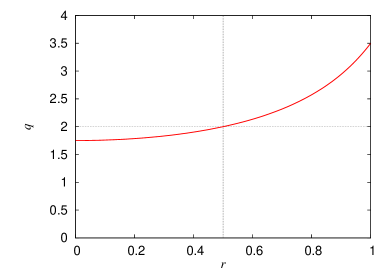
Figure 1: The safety factor profile $q(r)$ for a stationary state.

The stationary state shown in figure 1 is unstable against a tearing mode with mode numbers $m=-2$ and $n=1$, which has the tearing mode parameter[35] $\Delta^{\prime}\approx 22.4$. Thus a small perturbation with $m=-2$ and $n=1$ was added to the cylindrically symmetric state, giving a radial magnetic field across the $q=2$ surface. The radial profiles of the $m=-2$ and $n=1$ components are shown in figure 2.

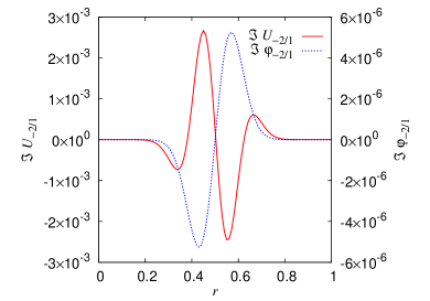
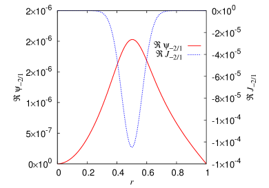
Figure 2: Depiction of $m=-2$ and $n=1$ components of (a) $\Im U$ and $\Im\varphi$, (b) $\Re\psi$ and $\Re J$ at $t=0$. A radial magnetic field exists at the $q=2$ surface.

Let us compare our three smoothing kernels. For the initial condition shown in figures 1 and 2, the right-hand sides of the evolution equations are plotted in figure 3. For SA-2 and SA-3, the amplitudes of the plotted figures are multiplied by $10$ and $100$, respectively for easier comparison. Observe in figure 3 how the $r$-dependence is smoother for SA-3.

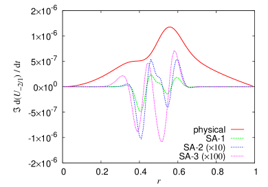
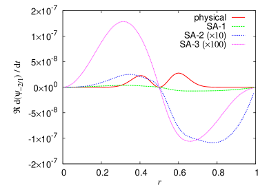
Figure 3: Depiction of $m=-2$ and $n=1$ components of (a) $\Im\frac{{\rm d}U_{-2/1}}{{\rm d}t}$ and (b) $\Re\frac{{\rm d}\psi_{-2/1}}{{\rm d}t}$ at $t=0$ for physical dynamics and SA. Since the amplitudes are largely different, those of SA-2 and SA-3 are multiplied by $10$ and $100$, respectively. The significant smoothing effect in $r$ of SA-3 is observed in (a).

Figure 4 shows the radial profile of $g_{m/n,-m/-n}(r,r^{\prime\prime})$ of SA-3 for $r^{\prime\prime}=0.2$, $0.4$, $0.6$ and $0.8$. The mode numbers are $m=-2$ and $n=1$ in figure 4, and $m=-10$ and $n=5$ in figure 4. The range of the vertical axis is the same for both figures. Note that $g_{m/n,-m/-n}(r,r^{\prime\prime})$ has smaller amplitudes for high $m$ and $n$. This smoothing effect in 2D is the same as that observed in [27, 22, 23], and is present also in SA-2. As for the smoothing effect in $r$, it is larger for smaller $m$ and $n$ because the radial extent of $g_{m/n,-m/-n}(r,r^{\prime\prime})$ is larger for smaller $m$ and $n$. Note that there is no smoothing effect in $r$ if $g_{m/n,-m/-n}(r,r^{\prime\prime})=\delta(r-r^{\prime\prime})$, as in SA-2. Thus the smoothing effect in $r$ of SA-3 may disappear if $m$ and $n$ go to infinity, while the smoothing in $\theta$ and $\zeta$ becomes infinitely large.

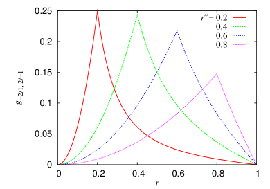
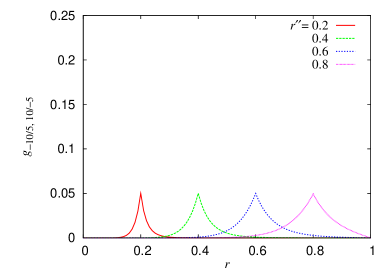
Figure 4: Radial profile plots of the 3D Green’s functions $g_{m/n,-m/-n}(r,r^{\prime\prime})$ of SA-3 with (a) $m=-2$, $n=1$ and (b) $m=-10$ and $n=5$, for $r^{\prime\prime}=0.2$, $0.4$, $0.6$ and $0.8$. The amplitudes of $g_{m/n,-m/-n}(r,r^{\prime\prime})$ are smaller for larger $m$ and $n$, implying a larger smoothing effect. Also, observe the larger smoothing in $r$ for smaller $m$ and $n$, since the radial extent of $g_{m/n,-m/-n}(r,r^{\prime\prime})$ is larger for smaller $m$ and $n$.

The time evolution of the energy and the conserved quantities are shown in figure 5 with $\alpha_{UU}=\alpha_{\psi\psi}=100$ for SA-2 and SA-3. SA-1 was numerically unstable, and a stationary state was not obtained. From figure 5, we observe that the total energy $E_{\rm k}+E_{\rm m}$ decreases monotonically. Figure 5 shows the time history of $\displaystyle{{|{\rm d}E_{\rm k}/{\rm d}t|}/{E_{\rm k}}}$ and $\displaystyle{{|{\rm d}E_{\rm m}/{\rm d}t|}/{E_{\rm m}}}$. When they became lower than the tolerance $10^{-6}$, the simulation was stopped. Since the magnetic energy $E_{\rm m}$ is dominant, its change is relatively small from the beginning. From figures 5, 5 and 5, we observe that quantities that should be conserved are well conserved in the simulation. The change of $C_{\rm m}$ is monitored relatively to its initial value $C_{\rm m}(0)=3.76$, while $C_{\rm v}$ and $C_{\rm c}$ are plotted directly since their initial values are zero.

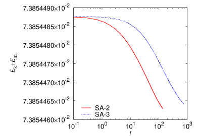
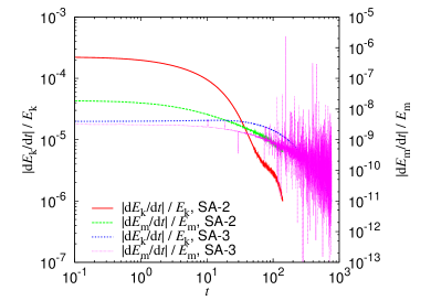
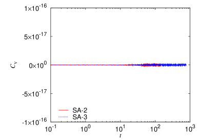
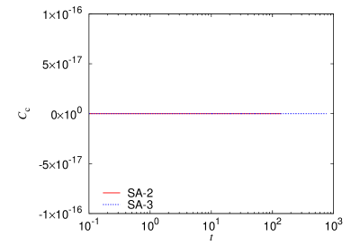
Figure 5: Time evolution of (a) total energy $E_{\rm k}+E_{\rm m}$, (b) relative change rate of energy $|{\rm d}E_{\rm k}/{\rm d}t|/E_{\rm k}$ and $|{\rm d}E_{\rm m}/{\rm d}t|/E_{\rm m}$, (c) relative change $(C_{\rm m}(t)-C_{\rm m}(0))/C_{\rm m}(0)$, (d) $C_{\rm v}$ and (e) $C_{\rm c}$. The values $\alpha_{UU}=\alpha_{\psi\psi}=100$ were used. The total energy decreases monotonically and reaches a stationary state. The relative change of $C_{\rm m}$ is normalized by the initial value $C_{\rm m}(0)$ in (c). Since $C_{\rm v}=0$ and $C_{\rm c}=0$ at $t=0$, just their values themselves are plotted in (d) and (e).

SA-3 requires longer $t$ for convergence. Although the time $t$ is not physical and depends on $\alpha_{UU}$ and $\alpha_{\psi\psi}$, late convergence can also be because SA-3 smooths in $r$, and thus tends to prevent generation of fine structure in $r$. Magnetic islands have current channels that may be easier to generate with SA-2 than SA-3. This also indicates that a stationary state with fine structure in $\theta$ and $\zeta$ may take more simulation time using SA-2 and SA-3.

Figure 6 shows the real parts of the radial profiles $\Re\psi_{-2/1}$, $\Re\psi_{-4/2}$, $\Re J_{-2/1}$ and $\Re J_{-4/2}$ of the obtained stationary state. The radial magnetic field of the $m=-2$ and $n=1$ mode remains at the $q=2$ surface when the magnetic island exists. These profiles differ greatly from the initial condition, with larger amplitudes, while the radial profile of the $m/n=-2/1$ mode is still similar to the corresponding linear mode. Therefore, the magnetic island of this stationary state saturated in a weakly nonlinear sense.

On the other hand, the radial profiles of SA-2 and SA-3 are a bit different. Also, almost no change was observed in $\Im U$ and $\Im\varphi$. These will be discussed in the next section.

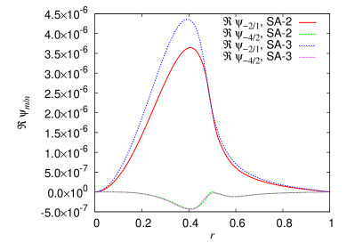
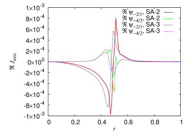
Figure 6: Radial profiles of (a) $\Re\psi_{-2/1}$ and $\Re\psi_{-4/2}$ and (b) $\Re J_{-2/1}$ and $\Re J_{-4/2}$ of the obtained stationary state are plotted. Almost no changes occur in $\Im U$ and $\Im\varphi$. The $m/n=-2/1$ components have similar structure as the linear mode.

4 Discussion

Firstly, let us investigate why SA-2 and SA-3 differ. One reason could be the tolerance for stopping the simulation, which was set to $\displaystyle{|{\rm d}E_{\rm k}/{\rm d}t|/E_{\rm k}}$ and $\displaystyle{|{\rm d}E_{\rm m}/{\rm d}t|/E_{\rm m}}$ becoming smaller than $10^{-6}$. While the magnetic energy of the $m/n=0/0$ component is very large, the relative rate of change of $E_{\rm m}$ of the $m/n\neq 0/0$ components was very small. Therefore, we may need another criterion for convergence. For example, separating out the energy of the $m/n=0/0$ mode and monitoring the relative change rates of both components of energy could be an improvement.

Secondly, let us investigate why $\Im U$ and $\Im\varphi$ did not change during the SA evolution; i.e., why $\psi$ relaxed faster than $U$. One possible reason is again the convergence criterion. If a longer simulation is performed with a much smaller tolerance, $U$ and $\varphi$ may also change. Another possible reason may be due to the choice of $\alpha_{UU}$ and $\alpha_{\psi\psi}$, especially their ratio. If we write the evolution equations for SA-1 explicitly, we have

$$\frac{\partial U}{\partial t}=\alpha_{UU}[U(\bi{x}),f^{U}(\bi{x})]+\alpha_{\psi\psi}\left([\psi(\bi{x}),f^{\psi}(\bi{x})]-\varepsilon\frac{\partial f^{\psi}(\bi{x})}{\partial\zeta}\right),$$ (55)

$$\frac{\partial\psi}{\partial t}=\alpha_{\psi\psi}\left([\psi(\bi{x}),f^{U}(\bi{x})]-\varepsilon\frac{\partial f^{U}(\bi{x})}{\partial\zeta}\right).$$ (56)

Therefore, the ratio of $\alpha_{UU}$ to $\alpha_{\psi\psi}$ can significantly affect the time evolution of $U$. As was studied in [22] for the 2D cases, the relaxation path can change if we change the ratio of $\alpha_{UU}$ to $\alpha_{\psi\psi}$. As we observe, the time evolution of $U$ is governed by two advection fields $f^{U}$ and $f^{\psi}$, while $\psi$ by $f^{U}$ only. Therefore the relaxation path can change if we change the ratio of contributions from $f^{U}$ and $f^{\psi}$. This situation is also the same for SA-2 and SA-3. If the relaxation of $U$ is much slower than $\psi$, a simple solution is to increase the ratio of $\alpha_{UU}$ to $\alpha_{\psi\psi}$. Then the right-hand side of the evolution equation of $\psi$ becomes smaller and that of $U$ becomes larger. However, if $\alpha_{UU}$ is increased in the present code, the simulation tends to be unstable. The dependence of the numerical stability on $\alpha_{UU}$ and $\alpha_{\psi\psi}$, in addition to the choice of the symmetric bracket, needs to be examined more carefully.

The result of section 3 is only one example of a magnetic island stationary state achievable with SA. When the initial perturbation of the $m=-2$ and $n=1$ component was chosen larger, the $m=0$ and $n=0$ components of $U$ and $\psi$ were changed significantly by the nonlinear effects, leading to a different stationary state. Incorporating Dirac constraints as in [27] should be explored in the future for selecting out desired states. Also, the effects of the $m=0$ and $n=0$ component of the plasma rotation should be investigated because it changes the linear stability against tearing modes. Details of these issues will be studied and will be reported on in the near future.

5 Summary

The method of simulated annealing (SA) was developed to obtain a three-dimensional stationary state of low-beta reduced MHD in cylindrical geometry. The theory of SA was explained for low-beta reduced MHD, and three versions of the symmetric bracket were introduced. A simulation demonstrated that the energy of the system monotonically decreases by SA, while conserving other invariants. Starting from a cylindrically symmetric state with the addition of a perturbation that opens a small magnetic island at a rational surface, SA generated a stationary state with magnetic islands as a lower energy state. Smoothing effects by the symmetric brackets were also examined. A symmetric bracket with higher smoothing may require longer simulation time for convergence, while it can contribute to numerical stability. Several issues for consideration in the future were discussed.

References

References

- [1] R. Lüst and A. Schlüter, Zeitschrift für Naturforschüng 12A, 850 (1957).
- [2] V. D. Shafranov, Soviet Physics JETP 6, 545 (1958).
- [3] H. Grad and H. Rubin, in Proceedings of the Second United Nations International Conference on the Peaceful Uses of Atomic Energy (United Nations, Geneva, 1958), Vol. 31.
- [4] K. Lackner, Comput. Phys. Commun. 12, 33 (1976).
- [5] H. P. Zehrfeld, B. J. Green, Nucl. Fusion 12, 569 (1972).
- [6] B. J. Green, H. P. Zehrfeld, Nucl. Fusion 13, 750 (1973).
- [7] H. R. Strauss, Phys. Fluids 16, 1377 (1973).
- [8] L. Guazzotto, R. Betti, J. Manickam and S. Kaye, Phys. Plasmas 11, 604 (2004).
- [9] T. Takeda and S. Tokuda, J. Comput. Phys. 93, 1 (1991).
- [10] S. P. Hirshman and J. C. Whitson, Phys. Fluids 26, 3553 (1983).
- [11] S. P. Hirshman, W. I. Van Rij and P. Merkel, Comput. Phys. Commun. 43, 143 (1986).
- [12] A. H. Reiman and H. S. Greenside, Comput. Phys. Commun. 43, 157 (1986).
- [13] K. Harafuji, T. Hayashi and T. Sato, J. Comput. Phys. 81, 169 (1989).
- [14] Y. Suzuki, N. Nakajima et al., Nucl. Fusion 46, L19 (2006).
- [15] S. R. Hudson, R. L. Dewar et al., Plasma Phys. Control. Fusion 54, 014005 (2012).
- [16] J-k. Park, A. H. Boozer, A. H. Glasser, Phys. Plasmas 14, 052110 (2007).
- [17] Y. Suzuki, C. Hegna, and Y. Nakamura, in Proceedings of the 43rd EPS Conference on Plasma Physics (European Physical Society, Leuven, Belgium, 2016).
- [18] Y. Narushima, S. Sakakibara et al., Nucl. Fusion 55, 073004 (2015).
- [19] P. Martin et al., Nucl. Fusion 43, 1855 (2003).
- [20] W. F. Bergerson, F. Auriemma et al., Phys. Rev. Lett. 107, 255001 (2011).
- [21] P. Piovesan, D. Bonfiglio et al., Nucl. Fusion 6, 064006 (2014).
- [22] Y. Chikasue and M. Furukawa, Phys. Plasmas 22, 022511 (2015).
- [23] Y. Chikasue and M. Furukawa, J. Fluid Mech. 774, 443 (2015).
- [24] G. K. Vallis, G. F. Carnevale and W. R. Young, J. Fluid Mech. 207, 133 (1989).
- [25] G. F. Carnevale and G. K. Vallis, J. Fluid Mech. 213, 549 (1990).
- [26] T. G. Shepherd, J. Fluid Mech. 213, 573 (1990).
- [27] G. R. Flierl, P. J. Morrison, Physica D 240, 212 (2011).
- [28] P. J. Morrison and J. M. Greene, Phys. Rev. Lett. 45, 790 (1980).
- [29] P. J. Morrison, Rev. Mod. Phys. 70, 467 (1998).
- [30] M. D. Kruskal and C. R. Oberman, Phys. Fluids 1, 275 (1958).
- [31] V. I. Arnol’d, Prikl. Math. Mech. 29, 846 (1965), [English transl. J. Appl. Maths Mech. 29, 1002–1008 (1965)].
- [32] H. R. Strauss, Phys. Fluids 19, 134 (1976).
- [33] P. J. Morrison and R. D. Hazeltine, Phys. Fluids 27, 886 (1984).
- [34] J. E. Marsden and P. J. Morrison, Contemp. Math 28, 133 (1984).
- [35] H. P. Furth, J. Killeen and M. N. Rosenbluth, Phys. Fluids 6, 459 (1963).