Convexified Convolutional Neural Networks

Abstract

We describe the class of convexified convolutional neural networks (CCNNs), which capture the parameter sharing of convolutional neural networks in a convex manner. By representing the nonlinear convolutional filters as vectors in a reproducing kernel Hilbert space, the CNN parameters can be represented as a low-rank matrix, which can be relaxed to obtain a convex optimization problem. For learning two-layer convolutional neural networks, we prove that the generalization error obtained by a convexified CNN converges to that of the best possible CNN. For learning deeper networks, we train CCNNs in a layer-wise manner. Empirically, CCNNs achieve performance competitive with CNNs trained by backpropagation, SVMs, fully-connected neural networks, stacked denoising auto-encoders, and other baseline methods.

1 Introduction

Convolutional neural networks (CNNs) [28] have proven successful across many tasks in machine learning and artificial intelligence, including image classification [28, 25], face recognition [26], speech recognition [21], text classification [45], and game playing [32, 37]. There are two principal advantages of a CNN over a fully-connected neural network: (i) sparsity—that each nonlinear convolutional filter acts only on a local patch of the input, and (ii) parameter sharing—that the same filter is applied to each patch.

However, as with most neural networks, the standard approach to training CNNs is based on solving a nonconvex optimization problem that is known to be NP-hard [6]. In practice, researchers use some flavor of stochastic gradient method, in which gradients are computed via backpropagation [7]. This approach has two drawbacks: (i) the rate of convergence, which is at best only to a local optimum, can be slow due to nonconvexity (for instance, see the paper [19]), and (ii) its statistical properties are very difficult to understand, as the actual performance is determined by some combination of the CNN architecture along with the optimization algorithm.

In this paper, with the goal of addressing these two challenges, we propose a new model class known as convexified convolutional neural networks (CCNNs). These models have two desirable features. First, training a CCNN corresponds to a convex optimization problem, which can be solved efficiently and optimally via a projected gradient algorithm. Second, the statistical properties of CCNN models can be studied in a precise and rigorous manner. We obtain CCNNs by convexifying two-layer CNNs; doing so requires overcoming two challenges. First, the activation function of a CNN is nonlinear. In order to address this issue, we relax the class of CNN filters to a reproducing kernel Hilbert space (RKHS). This approach is inspired by our earlier work [48], involving a subset of the current authors, in which we developed this relaxation step for fully-connected neural networks. Second, the parameter sharing induced by CNNs is crucial to its effectiveness and must be preserved. We show that CNNs with RKHS filters can be parametrized by a low-rank matrix. Further relaxing the low-rank constraint to a nuclear norm constraint leads to our final formulation of CCNNs.

On the theoretical front, we prove an oracle inequality on generalization error achieved by our class of CCNNs, showing that it is upper bounded by the best possible performance achievable by a two-layer CNN given infinite data—a quantity to which we refer as the oracle risk—plus a model complexity term that decays to zero polynomially in the sample size. Our results show that the sample complexity for CCNNs is significantly lower than that of the convexified fully-connected neural network [48], highlighting the importance of parameter sharing. For models with more than one hidden layer, our theory does not apply, but we provide encouraging empirical results using a greedy layer-wise training heuristic. We then apply CCNNs to the MNIST handwritten digit dataset as well as four variation datasets [43], and find that it achieves the state-of-the-art performance. On the CIFAR-10 dataset, CCNNs outperform CNNs of the same depths, as well as other baseline methods that do not involve nonconvex optimization. We also demonstrate that building CCNNs on top of existing CNN filters improves the performance of CNNs.

The remainder of this paper is organized as follows. We begin in Section 2 by introducing convolutional neural networks, and setting up the empirical risk minimization problem studied in this paper. In Section 3, we describe the algorithm for learning two-layer CCNNs, beginning with the simple case of convexifying CNNs with a linear activation function, then proceeding to convexify CNNs with a nonlinear activation. We show that the generalization error of a CCNN converges to that of the best possible CNN. In Section 4, we describe several extensions to the basic CCNN algorithm, including averaging pooling, multi-channel input processing, and the layer-wise learning of multi-layer CNNs. In Section 5, we report the empirical evaluations of CCNNs. We survey related work in Section 6 and conclude the paper in Section 7.

Notation.

For any positive integer $n$, we use $[n]$ as a shorthand for the discrete set $\{1,2,\dots,n\}$. For a rectangular matrix $A$, let $\|{A}\|_{*}$ be its nuclear norm, $\|{A}\|_{2}$ be its spectral norm (i.e., maximal singular value), and $\|{A}\|_{\rm\scriptsize{F}}$ be its Frobenius norm. We use $\ell^{2}(\mathbb{N})$ to denote the set of countable dimensional vectors $v=(v_{1},v_{2},\dots)$ such that $\sum_{\ell=1}^{\infty}v_{\ell}^{2}<\infty$. For any vectors $u,v\in\ell^{2}(\mathbb{N})$, the inner product $\langle u,\,v\rangle:=\sum_{\ell=1}^{\infty}u_{i}v_{i}$ and the $\ell_{2}$-norm $\|{u}\|_{2}:=\sqrt{\langle u,\,u\rangle}$ are well defined.

2 Background and problem set-up

In this section, we formalize the class of convolutional neural networks to be learned and describe the associated nonconvex optimization problem.

2.1 Convolutional neural networks.

At a high level, a two-layer CNN is a particular type of function that maps an input vector $x\in{\mathbb{R}}^{d_{0}}$ (e.g., an image) to an output vector in $y\in{\mathbb{R}}^{d_{2}}$ (e.g., classification scores for the $d_{2}$ classes). This mapping is formed in the following manner:

• First, we extract a collection of $P$ vectors $\{z_{p}(x)\}_{j=1}^{P}$ of the full input vector $x$. Each vector $z_{p}(x)\in\mathbb{R}^{d_{1}}$ is referred to as a patch, and these patches may depend on overlapping components of $x$.

• Second, given some choice of activation function $\sigma:\mathbb{R}\rightarrow\mathbb{R}$ and a collection of weight vectors $\{w_{j}\}_{j=1}^{r}$ in $\mathbb{R}^{d_{1}}$, we compute the functions

  $$h_{j}(z):=\sigma(w_{j}^{\top}z)\quad\mbox{for each patch $z\in{\mathbb{R}}^{d_{1}}$.}$$ (1)

  Each function $h_{j}$ (for $j\in[r]$) is known as a filter, and note that the same filters are applied to each patch—this corresponds to the parameter sharing of a CNN.

• Third, for each patch index $p\in[P]$, filter index $j\in[r]$, and output coordinate $k\in[d_{2}]$, we introduce a coefficient $\alpha_{k,j,p}\in\mathbb{R}$ that governs the contribution of the filter $h_{j}$ on patch $z_{p}(x)$ to output $f_{k}(x)$. The final form of the CNN is given by $f(x):\,=(f_{1}(x),\dots,f_{d_{2}}(x))$, where the $k^{th}$ component is given by

  $$f_{k}(x):=\sum_{j=1}^{r}\sum_{p=1}^{P}\alpha_{k,j,p}h_{j}(z_{p}(x)).$$ (2)

Taking the patch functions $\{z_{p}\}_{p=1}^{P}$ and activation function $\sigma$ as fixed, the parameters of the CNN are the filter vectors $\mathbf{w}:=\{w_{j}\in\mathbb{R}^{d_{1}}:\;j\in[r]\}$ along with the collection of coefficient vectors $\boldsymbol{\alpha}:=\{\alpha_{k,j}\in\mathbb{R}^{P}:\;k\in[d_{2}],j\in[r]\}$. We assume that all patch vectors $z_{p}(x)\in{\mathbb{R}}^{d_{1}}$ are contained in the unit $\ell_{2}$-ball. This assumption can be satisfied without loss of generality by normalization: By multiplying a constant $\gamma>0$ to every patch $z_{p}(x)$ and multiplying $1/\gamma$ to the filter vectors $\mathbf{w}$, the assumption will be satisfied without changing the the output of the network.

Given some positive radii $B_{1}$ and $B_{2}$, we consider the model class

$$\mathcal{F}_{\text{cnn}}(B_{1},B_{2}) :=\Big{\{}\mbox{$f$ of the form~{}\eqref{eqn:def-cnn}}:\;\mbox{$\max\limits_{j\in[r]}\|w_{j}\|_{2}\leq B_{1}$ and $\max\limits_{k\in[d_{2}],j\in[r]}\|\alpha_{k,j}\|_{2}\leq B_{2}$}\Big{\}}.$$ (3)

When the radii $(B_{1},B_{2})$ are clear from context, we adopt $\mathcal{F}_{\text{cnn}}$ as a convenient shorthand.

2.2 Empirical risk minimization.

Given an input-output pair $(x,y)$ and a CNN $f$, we let $\mathcal{L}(f(x);y)$ denote the loss incurred when the output $y$ is predicted via $f(x)$. We assume that the loss function $\mathcal{L}$ is convex and $L$-Lipschitz in its first argument given any value of its second argument. As a concrete example, for multiclass classification with $d_{2}$ classes, the output vector $y$ takes values in the discrete set $[d_{2}]=\{1,2,\ldots,d_{2}\}$. For example, given a vector $f(x)=(f_{1}(x),\ldots,f_{d_{2}}(y))\in\mathbb{R}^{d_{2}}$ of classification scores, the associated multiclass logistic loss for a pair $(x,y)$ is given by $\mathcal{L}(f(x);y):=-f_{y}(x)+\log\big{(}\sum_{y^{\prime}=1}^{d_{2}}\exp(f_{y^{\prime}}(x))\big{)}$.

Given $n$ training examples $\{(x_{i},y_{i})\}_{i=1}^{n}$, we would like to compute an empirical risk minimizer

$$\widehat{f}_{\text{cnn}}\in\arg\min_{f\in\mathcal{F}_{\text{cnn}}}\sum_{i=1}^{n}\mathcal{L}(f(x_{i});y_{i}).$$ (4)

Recalling that functions $f\in\mathcal{F}_{\text{cnn}}$ depend on the parameters $\mathbf{w}$ and $\boldsymbol{\alpha}$ in a highly nonlinear way (2), this optimization problem is nonconvex. As mentioned earlier, heuristics based on stochastic gradient methods are used in practice, which makes it challenging to gain a theoretical understanding of their behavior. Thus, in the next section, we describe a relaxation of the class $\mathcal{F}_{\text{cnn}}$ that allows us to obtain a convex formulation of the associated empirical risk minimization problem.

3 Convexifying CNNs

We now turn to the development of the class of convexified CNNs. We begin in Section 3.1 by illustrating the procedure for the special case of the linear activation function. Although the linear case is not of practical interest, it provides intuition for our more general convexification procedure, described in Section 3.2, which applies to nonlinear activation functions. In particular, we show how embedding the nonlinear problem into an appropriately chosen reproducing kernel Hilbert space (RKHS) allows us to again reduce to the linear setting.

3.1 Linear activation functions: low rank relaxations

In order to develop intuition for our approach, let us begin by considering the simple case of the linear activation function $\sigma(t)=t$. In this case, the filter $h_{j}$ when applied to the patch vector $z_{p}(x)$ outputs a Euclidean inner product of the form $h_{j}(z_{p}(x))=\langle z_{p}(x),\,w_{j}\rangle$. For each $x\in\mathbb{R}^{d_{0}}$, we first define the $P\times d_{1}$-dimensional matrix

$$Z(x) :=\begin{bmatrix}z_{1}(x)^{\top}\\ \vdots\\ z_{P}(x)^{\top}\end{bmatrix}.$$ (5)

We also define the $P$-dimensional vector $\alpha_{k,j}:=(\alpha_{k,j,1},\dots,\alpha_{k,j,P})^{\top}$. With this notation, we can rewrite equation (2) for the $k^{th}$ output as

$$f_{k}(x)=\sum_{j=1}^{r}\sum_{p=1}^{P}\alpha_{k,j,p}\langle z_{p}(x),\,w_{j}\rangle=\sum_{j=1}^{r}\alpha_{k,j}^{\top}Z(x)w_{j}={\rm tr}\Big{(}Z(x)\Big{(}\sum_{j=1}^{r}w_{j}\alpha_{k,j}^{\top}\Big{)}\Big{)}={\rm tr}(Z(x)A_{k}),$$ (6)

where in the final step, we have defined the $d_{1}\times P$-dimensional matrix $A_{k}:=\sum_{j=1}^{r}w_{j}\alpha_{k,j}^{\top}$. Observe that $f_{k}$ now depends linearly on the matrix parameter $A_{k}$. Moreover, the matrix $A_{k}$ has rank at most $r$, due to the parameter sharing of CNNs. See Figure 1 for a graphical illustration of this model structure.

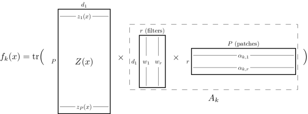
Figure 1: The $k^{th}$ output of a CNN $f_{k}(x)\in\mathbb{R}$ can be expressed as the product between a matrix $Z(x)\in\mathbb{R}^{P\times d_{1}}$ whose rows are features of the input patches and a rank-$r$ matrix $A_{k}\in\mathbb{R}^{d_{1}\times P}$, which is made up of the filter weights $\{w_{j}\}$ and coefficients $\{a_{k,j,p}\}$, as illustrated. Due to the parameter sharing intrinsic to CNNs, the matrix $A_{k}$ inherits a low rank structure, which can be enforced via convex relaxation using the nuclear norm.

Letting $A:=(A_{1},\dots,A_{d_{2}})$ be a concatenation of these matrices across all $d_{2}$ output coordinates, we can then define a function $f^{A}:\mathbb{R}^{d_{1}}\rightarrow\mathbb{R}^{d_{2}}$ of the form

$$f^{A}(x) :=({\rm tr}(Z(x)A_{1}),\dots,{\rm tr}(Z(x)A_{d_{2}})).$$ (7)

Note that these functions have a linear parameterization in terms of the underlying matrix $A$. Our model class corresponds to a collection of such functions based on imposing certain constraints on the underlying matrix $A$: in particular, we define

$$\mathcal{F}_{\text{cnn}}(B_{1},B_{2}) :=\Big{\{}f^{A}:\;\underbrace{\mbox{$\max\limits_{j\in[r]}\|{w_{j}}\|_{2}\leq B_{1}$ and $\max\limits_{\begin{subarray}{c}k\in[d_{2}]\\ j\in[r]\end{subarray}}\|{\alpha_{k,j}}\|_{2}\leq B_{2}$}}_{\mbox{Constraint (C1)}}\quad\mbox{and}\underbrace{\mbox{$\text{rank}(A)=r$}}_{\mbox{Constraint (C2)}}\Big{\}}.$$

This is simply an alternative formulation of our original class of CNNs. Notice that if the filter weights $w_{j}$ are not shared across all patches, then the constraint (C1) still holds, but constraint (C2) no longer holds. Thus, the parameter sharing of CNNs is realized by the low-rank constraint (C2). The matrix $A$ of rank $r$ can be decomposed as $A=UV^{\top}$, where both $U$ and $V$ have $r$ columns. The column space of matrix $A$ contains the convolution parameters $\{w_{j}\}$, and the row space of $A$ contains to the output parameters $\{\alpha_{k,j}\}$.

The rank-$r$ matrices satisfying constraints (C1) and (C2) form a nonconvex set. A standard convex relaxation of a rank constraint is based on the nuclear norm $\|{A}\|_{*}$ corresponding to the sum of the singular values of $A$. It is straightforward to verify that any matrix $A$ satisfying the constraints (C1) and (C2) must have nuclear norm bounded as $\|{A}\|_{*}\leq B_{1}B_{2}r\sqrt{d_{2}}$. Consequently, if we define the function class

$$\mathcal{F}_{\text{ccnn}} :=\Big{\{}f^{A}:\;\|{A}\|_{*}\leq B_{1}B_{2}r\sqrt{d_{2}}\Big{\}},$$ (8)

then we are guaranteed that $\mathcal{F}_{\text{ccnn}}\supseteq\mathcal{F}_{\text{cnn}}$.

Overall, we propose to minimize the empirical risk (4) over $\mathcal{F}_{\text{ccnn}}$ instead of $\mathcal{F}_{\text{cnn}}$; doing so defines a convex optimization problem over this richer class of functions

$$\widehat{f}_{\text{ccnn}}:=\arg\min_{f^{A}\in\mathcal{F}_{\text{ccnn}}}\sum_{i=1}^{n}\mathcal{L}(f^{A}(x_{i});y_{i}).$$ (9)

In Section 3.3, we describe iterative algorithms that can be used to solve this form of convex program in the more general setting of nonlinear activation functions.

3.2 Nonlinear activations: RKHS filters

For nonlinear activation functions $\sigma$, we relax the class of CNN filters to a reproducing kernel Hilbert space (RKHS). As we show, this relaxation allows us to reduce the problem to the linear activation case.

Let $\mathcal{K}:{\mathbb{R}}^{d_{1}}\times{\mathbb{R}}^{d_{1}}\to{\mathbb{R}}$ be a positive semidefinite kernel function. For particular choices of kernels (e.g., the Gaussian RBF kernel) and some sufficiently smooth activation function $\sigma$, we are able to show that the filter $h:z\mapsto\sigma(\langle w,\,z\rangle)$ is contained in the RKHS induced by the kernel function $\mathcal{K}$. See Section 3.4 for the choice of the kernel function and the activation function. Let $S:=\{z_{p}(x_{i}):p\in[P],i\in[n]\}$ be the set of patches in the training dataset. The representer theorem then implies that for any patch $z_{p}(x_{i})\in S$, the function value can be represented by

$$h(z_{p}(x_{i}))=\sum_{(i^{\prime},p^{\prime})\in[n]\times[P]}c_{i^{\prime},p^{\prime}}k(z_{p}(x_{i}),z_{p^{\prime}}(x_{i^{\prime}}))$$ (10)

for some coefficients $\{c_{i^{\prime},p^{\prime}}\}_{(i^{\prime},p^{\prime})\in[n]\times[P]}$. Filters taking the form (10) are members of the RKHS, because they are linear combinations of basis functions $z\mapsto k(z,z_{p^{\prime}}(x_{i^{\prime}}))$. Such filters are parametrized by a finite set of coefficients, which can be estimated via empirical risk minimization.

Let $K\in{\mathbb{R}}^{nP\times nP}$ be the symmetric kernel matrix, where with rows and columns indexed by the example-patch index pair $(i,p)\in[n]\times[P]$. The entry at row $(i,p)$ and column $(i^{\prime},p^{\prime})$ of matrix $K$ is equal to $\mathcal{K}(z_{p}(x_{i}),z_{p^{\prime}}(x_{i^{\prime}}))$. So as to avoid re-deriving everything in the kernelized setting, we perform a reduction to the linear setting of Section 3.1. Consider a factorization $K=QQ^{\top}$ of the kernel matrix, where $Q\in{\mathbb{R}}^{nP\times m}$; one example is the Cholesky factorization with $m=nP$. We can interpret each row $Q_{(i,p)}\in{\mathbb{R}}^{m}$ as a feature vector in place of the original $z_{p}(x_{i})\in{\mathbb{R}}^{d_{1}}$, and rewrite equation (10) as

$$h(z_{p}(x_{i}))=\langle Q_{(i,p)},w\rangle\quad\mbox{where}\quad w:=\sum_{(i^{\prime},p^{\prime})}c_{i^{\prime},p^{\prime}}Q_{(i^{\prime},p^{\prime})}.$$

In order to learn the filter $h$, it suffices to learn the $m$-dimensional vector $w$. To do this, define patch matrices $Z(x_{i})\in{\mathbb{R}}^{P\times m}$ for each $i\in[n]$ so that its $p$-th row is $Q_{(i,p)}$. Then we carry out all of Section 3.1; solving the ERM gives us a parameter matrix $A\in{\mathbb{R}}^{m\times Pd_{2}}$. The only difference is that the $B_{1}$ norm constraint needs to be relaxed as well. See Appendix B for details.

At test time, given a new input $x\in{\mathbb{R}}^{d_{0}}$, we can compute a patch matrix $Z(x)\in{\mathbb{R}}^{P\times m}$ as follows:

• The $p$-th row of this matrix is the feature vector for patch $p$, which is equal to $Q^{\dagger}v(z_{p}(x))\in{\mathbb{R}}^{m}$. Here, for any patch $z$, the vector $v(z)$ is defined as a $nP$-dimensional vector whose $(i,p)$-th coordinate is equal to $\mathcal{K}(z,z_{p}(x_{i}))$. We note that if $x$ is an instance $x_{i}$ in the training set, then the vector $Q^{\dagger}v(z_{p}(x))$ is exactly equal to $Q_{(i,p)}$. Thus the mapping $Z(x)$ applies to both training and testing.

• We can then compute the predictor $f_{k}(x)={\rm tr}(Z(x)A_{k})$ via equation (6). Note that we do not explicitly need to compute the filter values $h_{j}(z_{p}(x))$ to compute the output under the CCNN.

Retrieving filters.

However, when we learn multi-layer CCNNs, we need to compute the filters explicitly. Recall from Section 3.1 that the column space of matrix $A$ corresponds to parameters of the convolutional layer, and the row space of $A$ corresponds to parameters of the output layer. Thus, once we obtain the parameter matrix $A$, we compute a rank-$r$ approximation $A\approx\widehat{U}\widehat{V}^{\top}$. Then set the $j$-th filter $h_{j}$ to the mapping

$$z\mapsto\langle\widehat{U}_{j},\,Q^{\dagger}v(z)\rangle\quad\mbox{for any patch $z\in{\mathbb{R}}^{d_{1}}$,}$$ (11)

where $\widehat{U}_{j}\in{\mathbb{R}}^{m}$ is the $j$-th column of matrix $\widehat{U}$, and $Q^{\dagger}v(z)$ represents the feature vector for patch $z$. The matrix $\widehat{V}^{\top}$ encodes parameters of the output layer, thus doesn’t appear in the filter expression (11). It is important to note that the filter retrieval is not unique, because the rank-$r$ approximation of the matrix $A$ is not unique. One feasible way is to form the singular value decomposition $A=U\Lambda V^{\top}$, then define $\widehat{U}$ to be the first $r$ columns of $U$, and define $\widehat{V}^{\top}$ to be the first $r$ rows of $\Lambda V^{\top}$.

When we apply all of the $r$ filters to all patches of an input $x\in{\mathbb{R}}^{d_{0}}$, the resulting output is $H(x):=\widehat{U}^{\top}(Z(x))^{\top}$ — this is an $r\times P$ matrix whose element at row $j$ and column $p$ is equal to $h_{j}(z_{p}(x))$.

3.3 Algorithm

Input: Data $\{(x_{i},y_{i})\}_{i=1}^{n}$, kernel function $\mathcal{K}$, regularization parameter $R>0$, number of filters $r$.

1. Construct a kernel matrix $K\in{\mathbb{R}}^{nP\times nP}$ such that the entry at column $(i,p)$ and row $(i^{\prime},p^{\prime})$ is equal to $\mathcal{K}(z_{p}(x_{i}),z_{p^{\prime}}(x_{i^{\prime}}))$. Compute a factorization $K=QQ^{\top}$ or an approximation $K\approx QQ^{\top}$, where $Q\in{\mathbb{R}}^{nP\times m}$.

2. For each $x_{i}$, construct patch matrix $Z(x_{i})\in{\mathbb{R}}^{P\times m}$ whose $p$-th row is the $(i,p)$-th row of $Q$, where $Z(\cdot)$ is defined in Section 3.2.

3. Solve the following optimization problem to obtain a matrix $\widehat{A}=(\widehat{A}_{1},\dots,\widehat{A}_{d_{2}})$:

   $$\widehat{A} \in\underset{\|{A}\|_{*}\leq R}{\rm argmin}\;\widetilde{\mathcal{L}}(A)\mbox{~{}~{}where~{}~{}}\widetilde{\mathcal{L}}(A):=\sum_{i=1}^{n}\mathcal{L}\Big{(}\big{(}{\rm tr}(Z(x_{i})A_{1}),\dots,{\rm tr}(Z(x_{i})A_{d_{2}})\big{)};y_{i}\Big{)}.$$ (12)

4. Compute a rank-$r$ approximation $\widetilde{A}\approx\widehat{U}\widehat{V}^{\top}$ where $\widehat{U}\in{\mathbb{R}}^{m\times r}$ and $\widehat{V}\in{\mathbb{R}}^{Pd_{2}\times r}$.

Output: Return the predictor $\widehat{f}_{\text{ccnn}}(x):=\big{(}{\rm tr}(Z(x)\widehat{A}_{1}),\dots,{\rm tr}(Z(x)\widehat{A}_{d_{2}})\big{)}$ and the convolutional layer output $H(x):=\widehat{U}^{\top}(Z(x))^{\top}$.

Algorithm 1 Learning two-layer CCNNs

The algorithm for learning a two-layer CCNN is summarized in Algorithm 1; it is a formalization of the steps described in Section 3.2. In order to solve the optimization problem (12), the simplest approach is to via projected gradient descent: At iteration $t$, using a step size $\eta^{t}>0$, it forms the new matrix $A^{t+1}$ based on the previous iterate $A^{t}$ according to:

$$A^{t+1}=\Pi_{R}\Big{(}A^{t}-\eta^{t}\;\nabla_{A}\widetilde{\mathcal{L}}(A^{t})\Big{)}.$$ (13)

Here $\nabla_{A}\widetilde{\mathcal{L}}$ denotes the gradient of the objective function defined in (12), and $\Pi_{R}$ denotes the Euclidean projection onto the nuclear norm ball $\{A:\|{A}\|_{*}\leq R\}$. This nuclear norm projection can be obtained by first computing the singular value decomposition of $A$, and then projecting the vector of singular values onto the $\ell_{1}$-ball. This latter projection step can be carried out efficiently by the algorithm of Duchi et al. [16]. There are other efficient optimization algorithms for solving the problem (12), such as the proximal adaptive gradient method [17] and the proximal SVRG method [46]. All these algorithms can be executed in a stochastic fashion, so that each gradient step processes a mini-batch of examples.

The computational complexity of each iteration depends on the width $m$ of the matrix $Q$. Setting $m=nP$ allows us to solve the exact kernelized problem, but to improve the computation efficiency, we can use Nyström approximation [15] or random feature approximation [33]; both are randomized methods to obtain a tall-and-thin matrix $Q\in{\mathbb{R}}^{nP\times m}$ such that $K\approx QQ^{\top}$. Typically, the parameter $m$ is chosen to be much smaller than $nP$. In order to compute the matrix $Q$, the Nyström approximation method takes $\mathcal{O}(m^{2}nP)$ time. The random feature approximation takes $\mathcal{O}(mnPd_{1})$ time, but can be improved to $\mathcal{O}(mnP\log d_{1})$ time using the fast Hadamard transform [27]. The complexity of computing a gradient vector on a batch of $b$ images is $\mathcal{O}(mPd_{2}b)$. The complexity of projecting the parameter matrix onto the nuclear norm ball is $\mathcal{O}(\min\{m^{2}Pd_{2},mP^{2}d_{2}^{2}\})$. Thus, the approximate algorithms provide substantial speed-ups on the projected gradient descent steps.

3.4 Theoretical results

In this section, we upper bound the generalization error of Algorithm 1, proving that it converges to the best possible generalization error of CNN. We focus on the binary classification case where the output dimension is $d_{2}=1$.

The learning of CCNN requires a kernel function $\mathcal{K}$. We consider kernel functions whose associated RKHS is large enough to contain any function taking the following form: $z\mapsto q(\langle w,z\rangle)$, where $q$ is an arbitrary polynomial function and $w\in{\mathbb{R}}^{d_{1}}$ is an arbitrary vector. As a concrete example, we consider the inverse polynomial kernel:

$$\mathcal{K}(z,z^{\prime}) :=\frac{1}{2-\langle z,\,z^{\prime}\rangle},\qquad\|{z}\|_{2}\leq 1,\|{z^{\prime}}\|_{2}\leq 1.$$ (14)

This kernel was studied by Shalev-Shwartz et al. [36] for learning halfspaces, and by Zhang et al. [48] for learning fully-connected neural networks. We also consider the Gaussian RBF kernel:

$$\mathcal{K}(z,z^{\prime}) :=\exp(-\gamma\|{z-z^{\prime}}\|_{2}^{2}),\qquad\|{z}\|_{2}=\|{z^{\prime}}\|_{2}=1,\gamma>0.$$ (15)

As we show in Appendix A, the inverse polynomial kernel and the Gaussian kernel satisfy the above notion of richness. We focus on these two kernels for the theoretical analysis.

Let $\widehat{f}_{\text{ccnn}}$ be the CCNN that minimizes the empirical risk (12) using one of the two kernels above. Our main theoretical result is that for suitably chosen activation functions, the generalization error of $\widehat{f}_{\text{ccnn}}$ is comparable to that of the best CNN model. In particular, the following theorem applies to activation functions $\sigma$ of the following types:

1. arbitrary polynomial functions (e.g., used by [10, 29]).

2. sinusoid activation function $\sigma(t):=\sin(t)$ (e.g., used by [39, 22]).

3. erf function $\sigma_{\tiny\rm erf}(t):=2/\sqrt{\pi}\int_{0}^{t}e^{-z^{2}}dz$, which represents an approximation to the sigmoid function (See Figure 2(a)).

4. a smoothed hinge loss $\sigma_{\rm sh}(t):=\int_{-\infty}^{t}\frac{1}{2}(\sigma_{\tiny\rm erf}(z)+1)dz$, which represents an approximation to the ReLU function (See Figure 2(b)).

To understand why these activation functions pair with our choice of kernels, we consider polynomial expansions of the above activation functions: $\sigma(t)=\sum_{j=0}^{\infty}a_{j}t^{j}$, and note that the smoothness of these functions are characterized by the rate of their coefficients $\{a_{j}\}_{j=0}^{\infty}$ converging to zero. If $\sigma$ is a polynomial in category (a), then the richness of the RKHS guarantees that it contains the class of filters activated by function $\sigma$. If $\sigma$ is a non-polynomial function in categories (b),(c),(d), then as Appendix A shows, the RKHS contains the filter only if the coefficients $\{a_{j}\}_{j=0}^{\infty}$ converge quickly enough to zero (the criterion depends on the choice of the kernel). Concretely, the inverse polynomial kernel is shown to capture all of the four categories of activations: they are referred as valid activation functions for the inverse polynomial kernel. The Gaussian kernel induces a smaller RKHS, and is shown to capture categories (a),(b), so that these functions are referred as valid activation functions for the Gaussian kernel. In contrast, the sigmoid function and the ReLU function are not valid for either kernel, because their polynomial expansions fail to converge quickly enough, or more intuitively speaking, because they are not smooth enough functions to be contained in the RKHS.

We are ready to state the main theoretical result. In the theorem statement, we use $K(X)\in{\mathbb{R}}^{P\times P}$ to denote the random kernel matrix obtained from an input vector $X\in\mathbb{R}^{d_{0}}$ drawn randomly from the population. More precisely, the $(p,q)$-th entry of $K(X)$ is given by $\mathcal{K}(z_{p}(X),z_{q}(X))$.

Theorem 1.

Assume that the loss function $\mathcal{L}(\cdot;y)$ is $L$-Lipchitz continuous for every $y\in[d_{2}]$ and that $\mathcal{K}$ is the inverse polynomial kernel or the Gaussian kernel. For any valid activation function $\sigma$, there is a constant $C_{\sigma}(B_{1})$ such that with the radius $R:=C_{\sigma}(B_{1})B_{2}r$, the expected generalization error is at most

$$\mathbb{E}_{X,Y}[\mathcal{L}(\widehat{f}_{\text{ccnn}}(X);Y)]\leq\inf_{f\in\mathcal{F}_{\text{cnn}}}\mathbb{E}_{X,Y}[\mathcal{L}(f(X);Y)]+\frac{c\;LC_{\sigma}(B_{1})B_{2}r\sqrt{\log(nP)\;\mathbb{E}_{X}[\|{K(X)}\|_{2}]}}{\sqrt{n}},$$ (16)

where $c>0$ is a universal constant.

Proof sketch

The proof of Theorem 1 consists of two parts: First, we consider a larger function class that contains the class of CNNs. This function class is defined as:

$$\mathcal{F}_{\text{ccnn}}:=\Big{\{}x\mapsto\sum_{j=1}^{r^{*}}\sum_{p=1}^{P}\alpha_{j,p}h_{j}(z_{p}(x)):\;r^{*}<\infty\mbox{ and }\sum_{j=1}^{r^{*}}\|{\alpha_{j}}\|_{2}\|{h_{j}}\|_{\mathcal{H}}\leq C_{\sigma}(B_{1})B_{2}d_{2}\Big{\}}.$$

where $\|{\cdot}\|_{\mathcal{H}}$ is the norm of the RKHS associated with the kernel. This new function class relaxes the class of CNNs in two ways: 1) the filters are relaxed to belong to the RKHS, and 2) the $\ell_{2}$-norm bounds on the weight vectors are replaced by a single constraint on $\|{\alpha_{j}}\|_{2}$ and $\|{h_{j}}\|_{\mathcal{H}}$. We prove the following property for the predictor $\widehat{f}_{\text{ccnn}}$: it must be an empirical risk minimizer of $\mathcal{F}_{\text{ccnn}}$, even though the algorithm has never explicitly optimized the loss within this nonparametric function class.

Second, we characterize the Rademacher complexity of this new function class $\mathcal{F}_{\text{ccnn}}$, proving an upper bound for it based on the matrix concentration theory. Combining this bound with the classical Rademacher complexity theory [4], we conclude that the generalization loss of $\widehat{f}_{\text{ccnn}}$ converges to the least possible generalization error of $\mathcal{F}_{\text{ccnn}}$. The later loss is bounded by the generalization loss of CNNs (because $\mathcal{F}_{\text{cnn}}\subseteq\mathcal{F}_{\text{ccnn}}$), which establishes the theorem. See Appendix C for the full proof of Theorem 1.

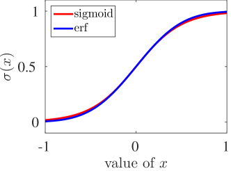
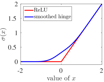
(a) sigmoid v.s. erf		(b) ReLU v.s. smoothed hinge loss

Figure 2: Comparing different activation functions. The two functions in (a) are quite similar. The smooth hinge loss in (b) is a smoothed version of ReLU.

Remark on activation functions.

It is worth noting that the quantity $C_{\sigma}(B_{1})$ depends on the activation function $\sigma$, and more precisely, depends on the convergence rate of the polynomial expansion of $\sigma$. Appendix A shows that if $\sigma$ is a polynomial function of degree $\ell$, then $C_{\sigma}(B_{1})=\mathcal{O}(B_{1}^{\ell})$. If $\sigma$ is the sinusoid function, the erf function or the smoothed hinge loss, then the quantity $C_{\sigma}(B_{1})$ will be exponential in $B_{1}$. In an algorithmic perspective, we don’t need to know the activation function for executing Algorithm 1. In a theoretical perspective, however, the choice of $\sigma$ is relevant from the point of Theorem 1 to compare $\widehat{f}_{\text{ccnn}}$ with the best CNN, whose representation power is characterized by the choice of $\sigma$. Therefore, if a CNN with a low-degree polynomial $\sigma$ performs well on a given task, then CCNN also enjoys correspondingly strong generalization. Empirically, this is actually borne out: in Section 5, we show that the quadratic activation function performs almost as well as the ReLU function for digit classification.

Remark on parameter sharing.

In order to demonstrate the importance of parameter sharing, consider a CNN without parameter sharing, so that we have filter weights $w_{j,p}$ for each filter index $j$ and patch index $p$. With this change, the new CNN output (2) is

$$f(x)=\sum_{j=1}^{r}\sum_{p=1}^{P}\alpha_{j,p}\sigma(w_{j,p}^{\top}z_{p}(x)),\quad\mbox{where $\alpha_{j,p}\in{\mathbb{R}}$ and $w_{j,p}\in{\mathbb{R}}^{d_{1}}$}.$$ (17)

Note that the hidden layer of this new network has $P$ times more parameters than that of the convolutional neural network with parameter sharing. These networks without parameter sharing can be learned by the recursive kernel method proposed by Zhang et al. [48]. This paper shows that under the norm constraints $\|{w_{j}}\|_{2}\leq B^{\prime}_{1}$ and $\sum_{j=1}^{r}\sum_{p=1}^{P}|\alpha_{j,p}|\leq B^{\prime}_{2}$, the excess risk of the recursive kernel method is at most $\mathcal{O}(LC_{\sigma}(B^{\prime}_{1})B^{\prime}_{2}\sqrt{K_{\max}/n})$, where $K_{\max}=\max_{z:\|{z}\|_{2}\leq 1}\mathcal{K}(z,z)$ is the maximal value of the kernel function. Plugging in the norm constraints of the function class $\mathcal{F}_{\text{cnn}}$, we have $B^{\prime}_{1}=B_{1}$ and $B^{\prime}_{2}=B_{2}r\sqrt{P}$. Thus, the expected risk of the estimated ${\widehat{f}}$ is bounded by:

$$\mathbb{E}_{X,Y}[\mathcal{L}({\widehat{f}}(X);Y)]\leq\inf_{f\in\mathcal{F}_{\text{cnn}}}\mathbb{E}_{X,Y}[\mathcal{L}(f(X);Y)]+\frac{c\;LC_{\sigma}(B_{1})B_{2}r\sqrt{PK_{\max}}}{\sqrt{n}}.$$ (18)

Comparing this bound to Theorem 1, we see that (apart from the logarithmic terms) they differ in the multiplicative factors of $\sqrt{P\,K_{\max}}$ versus $\sqrt{\mathbb{E}[\|{K(X)}\|_{2}]}$. Since the matrix $K(X)$ is $P$-dimensional, we have

$$\|{K(X)}\|_{2} \leq\max_{p\in[P]}\sum_{q\in[P]}|\mathcal{K}(z_{p}(X),z_{q}(X))|\leq P\,K_{\max}.$$

This demonstrates that $\sqrt{P\,K_{\max}}$ is always greater than $\sqrt{\mathbb{E}[\|{K(X)}\|_{2}]}$. In general, the first term can be up to factor of $\sqrt{P}$ times greater, which implies that the sample complexity of the recursive kernel method is up to $P$ times greater than that of the CCNN. This difference corresponds to the fact that the recursive kernel method learns a model with $P$ times more parameters. Although comparing the upper bounds doesn’t rigorously show that one method is better than the other, it gives the right intuition for understanding the importance of parameter sharing.

4 Learning multi-layer CCNNs

In this section, we describe a heuristic method for learning CNNs with more layers. The idea is to estimate the parameters of the convolutional layers incrementally from bottom to the top. Before presenting the multi-layer algorithm, we present two extensions, average pooling and multi-channel inputs.

Average pooling.

Average pooling is a technique to reduce the output dimension of the convolutional layer from dimensions $P\times r$ to dimensions $P^{\prime}\times r$ with $P^{\prime}<P$. Suppose that the filter $h_{j}$ applied to all the patch vectors produces the output vector $H_{j}(x):=(h_{j}(z_{1}(x)),\cdots,h_{j}(z_{P}(x)))\in{\mathbb{R}}^{P\times r}$. Average pooling produces a $P^{\prime}\times r$ matrix, where each row is the average of the rows corresponding to a small subset of the $P$ patches. For example, we might average every pair of adjacent patches, which would produce $P^{\prime}=P/2$ rows. The operation of average pooling can be represented via left-multiplication using a fixed matrix $G\in{\mathbb{R}}^{P^{\prime}\times P}$.

For the CCNN model, if we apply average pooling after the convolutional layer, then the $k$-th output of the CCNN model becomes ${\rm tr}(GZ(x)A_{k})$ where $A_{k}\in{\mathbb{R}}^{m\times P^{\prime}}$ is the new (smaller) parameter matrix. Thus, performing a pooling operation requires only replacing every matrix $Z(x_{i})$ in problem (12) by the pooled matrix $GZ(x_{i})$. Note that the linearity of the CCNN allows us to effectively pool before convolution, even though for the CNN, pooling must be done after applying the nonlinear filters. The resulting ERM problem is still convex, and the number of parameters have been reduced by $P/P^{\prime}$-fold. Although average pooling is straightforward to incorporate in our framework, unfortunately, max pooling does not fit into our framework due to its nonlinearity.

Processing multi-channel inputs.

If our input has $C$ channels (corresponding to RGB colors, for example), then the input becomes a matrix $x\in{\mathbb{R}}^{C\times d_{0}}$. The $c$-th row of matrix $x$, denoted by $x[c]\in{\mathbb{R}}^{d_{0}}$, is a vector representing the $c$-th channel. We define the multi-channel patch vector as a concatenation of patch vectors for each channel:

$$z_{p}(x):=(z_{p}(x[1]),\dots,z_{p}(x[C]))\in{\mathbb{R}}^{Cd_{1}}.$$

Then we construct the feature matrix $Z(x)$ using the concatenated patch vectors $\{z_{p}(x)\}_{p=1}^{P}$. From here, everything else of Algorithm 1 remains the same. We note that this approach learns a convex relaxation of filters taking the form $\sigma(\sum_{c=1}^{C}\langle w_{c},z_{p}(x[c])\rangle)$, parametrized by the vectors $\{w_{c}\}_{c=1}^{C}$.

Multi-layer CCNN.

Input:Data $\{(x_{i},y_{i})\}_{i=1}^{n}$, kernel function $\mathcal{K}$, number of layers $m$, regularization parameters $R_{1},\dots,R_{m}$, number of filters $r_{1},\dots,r_{m}$.

Define $H_{1}(x)=x$.

For each layer $s=2,\dots,m$:

• Train a two-layer network by Algorithm 1, taking $\{(H_{s-1}(x_{i}),y_{i})\}_{i=1}^{n}$ as training examples and $R_{s},r_{s}$ as parameters. Let $H_{s}$ be the output of the convolutional layer and ${\widehat{f}}_{s}$ be the predictor.

Output: Predictor ${\widehat{f}}_{m}$ and the top convolutional layer output $H_{m}$.

Algorithm 2 Learning multi-layer CCNNs

Given these extensions, we are ready to present the algorithm for learning multi-layer CCNNs. The algorithm is summarized in Algorithm 2. For each layer $s$, we call Algorithm 1 using the output of previous convolutional layers as input—note that this consists of $r$ channels (one from each previous filter) and thus we must use the multi-channel extension. Algorithm 2 outputs a new convolutional layer along with a prediction function, which is kept only at the last layer. We optionally use averaging pooling after each successive layer. to reduce the output dimension of the convolutional layers.

(a) rand		(b) rot
(c) img		(d) img+rot

Figure 3: Some variations of the MNIST dataset: (a) random background inserted into the digit image; (b) digits rotated by a random angle generated uniformly between $0$ and $2\pi$; (c) black and white image used as the background for the digit image; (d) combination of background perturbation and rotation perturbation.

5 Experiments

In this section, we compare the CCNN approach with other methods. The results are reported on the MNIST dataset and its variations for digit recognition, and on the CIFAR-10 dataset for object classification.

5.1 MNIST and variations

Since the basic MNIST digits are relatively easy to classify, we also consider more challenging variations [43]. These variations are known to be hard for methods without a convolution mechanism (for instance, see the paper [44]). Figure 3 shows a number of sample images from these different datasets. All the images are of size $28\times 28$. For all datasets, we use 10,000 images for training, 2,000 images for validation and 50,000 images for testing. This 10k/2k/50k partitioning is standard for MNIST variations [43].

Implementation details.

For the CCNN method and the baseline CNN method, we train two-layer and three-layer models respectively. The models with $k$ convolutional layers are denoted by CCNN-$k$ and CNN-$k$. Each convolutional layer is constructed on $5\times 5$ patches with unit stride, followed by $2\times 2$ average pooling. The first and the second convolutional layers contains 16 and 32 filters, respectively. The loss function is chosen as the $10$-class logistic loss. We use the Gaussian kernel $\mathcal{K}(z,z^{\prime})=\exp(-\gamma\|{z-z^{\prime}}\|_{2}^{2})$ and set hyperparameters $\gamma=0.2$ for the first convolutional layer and $\gamma=2$ for the second. The feature matrix $Z(x)$ is constructed via random feature approximation [33] with dimension $m=500$ for the first convolutional layer and $m=1000$ for the second. Before training each CCNN layer, we preprocess the input vectors $z_{p}(x_{i})$ using local contrast normalization and ZCA whitening [12]. The convex optimization problem is solved by projected SGD with mini-batches of size $50$.

As a baseline approach, the CNN models are activated by the ReLU function $\sigma(t)=\max\{0,t\}$ or the quadratic function $\sigma(t)=t^{2}$. We train them using mini-batch SGD. The input images are preprocessed by global contrast normalization and ZCA whitening [see, e.g. 40]. We compare our method against several alternative baselines. The CCNN-1 model is compared against an SVM with the Gaussian RBF kernel (SVM_rbf) and a fully connected neural network with one hidden layer (NN-1). The CCNN-2 model is compared against methods that report the state-of-the-art results on these datasets, including the translation-invariant RBM model (TIRBM) [38], the stacked denoising auto-encoder with three hidden layers (SDAE-3) [44], the ScatNet-2 model [8] and the PCANet-2 model [9].

Results.

	basic	rand	rot	img	img+rot
SVMrbf [44]	3.03%	14.58%	11.11%	22.61%	55.18%
NN-1 [44]	4.69%	20.04%	18.11%	27.41%	62.16%
CNN-1 (ReLU)	3.37%	9.83%	18.84%	14.23%	45.96%
CCNN-1	2.38%	7.45%	13.39%	10.40%	42.28%
TIRBM [38]	-	-	4.20%	-	35.50%
SDAE-3 [44]	2.84%	10.30%	9.53%	16.68%	43.76%
ScatNet-2 [8]	1.27%	12.30%	7.48%	18.40%	50.48%
PCANet-2 [9]	1.06%	6.19%	7.37%	10.95%	35.48%
CNN-2 (ReLU)	2.11%	5.64%	8.27%	10.17%	32.43%
CNN-2 (Quad)	1.75%	5.30%	8.83%	11.60%	36.90%
CCNN-2	1.38%	4.32%	6.98%	7.46%	30.23%

Table 1: Classification error on the basic MNIST and its four variations. The best performance within each block is bolded. The tag “ReLU” and “Quad” means ReLU activation and quadratic activation, respectively.

	Classification error
Full model CCNN-2	30.23%
Linear kernel	38.47%
No ZCA whitening	35.86%
Fewer random features	31.95%
$\|{A}\|_{\rm\scriptsize{F}}\leq R$ constraint	30.66%
Early stopping	30.63%

Table 2: Factors that affect the training of CCNN-2: changing the kernel function, removing the data whitening or decreasing the number of random features has non-negligible impact to the performance. The results are reported on the img+rot dataset.

Table 1 shows the classification errors on the test set. The models are grouped with respect to the number of layers that they contain. For models with one convolutional layer, the errors of CNN-1 are significantly lower than that of NN-1, highlighting the benefits of parameter sharing. The CCNN-1 model outperforms CNN-1 on all datasets. For models with two or more hidden layers, the CCNN-2 model outperforms CNN-2 on all datasets, and is competitive against the state-of-the-art. In particular, it achieves the best accuracy on the rand, img and img+rot dataset, and is comparable to the state-of-the-art on the remaining two datasets.

In order to understand the key factors that affect the training of CCNN filters, we evaluate five variants:

1. replace the Gaussian kernel by a linear kernel;

2. remove the ZCA whitening in preprocessing;

3. use fewer random features ($m=200$ rather than $m=500$) to approximate the kernel matrix;

4. regularize the parameter matrix by the Frobenius norm instead of the nuclear norm;

5. stop the mini-batch SGD early before it converges.

We evaluate the obtained filters by training a second convolutional layer on top of them, then evaluating the classification error on the hardest dataset img+rot. As Table 2 shows, switching to the linear kernel or removing the ZCA whitening significantly degenerates the performance. This is because that both variants equivalently modify the kernel function. Decreasing the number of random features also has a non-negligible effect, as it makes the kernel approximation less accurate. These observations highlight the impact of the kernel function. Interestingly, replacing the nuclear norm by a Frobenius norm or stopping the algorithm early doesn’t hurt the performance. To see their impact on the parameter matrix, we compute the effective rank (ratio between the nuclear norm and the spectral norm, see [18]) of matrix $\widehat{A}$. The effective rank obtained by the last two variants are equal to 77 and 24, greater than that of the original CCNN (equal to 12). It reveals that the last two variants have damaged the algorithm’s capability of enforcing a low-rank solution. However, the CCNN filters are retrieved from the top-$r$ singular vectors of the parameter matrix, hence the performance will remain stable as long as the top singular vectors are robust to the variation of the matrix.

In Section 3.4, we showed that if the activation function is a polynomial function, then the CCNN requires lower sample complexity to match the performance of the best possible CNN. More precisely, if the activation function is degree-$\ell$ polynomial, then $C_{\sigma}(B)$ in the upper bound will be controlled by $\mathcal{O}(B^{\ell})$. This motivates us to study the performance of low-degree polynomial activations. Table 1 shows that the CNN-2 model with a quadratic activation function achieves error rates comparable to that with a ReLU activation: CNN-2 (Quad) outperforms CNN-2 (ReLU) on the basic and rand datasets, and is only slightly worse on the rot and img dataset. Since the performance of CCNN matches that of the best possible CNN, the good performance of the quadratic activation in part explains why the CCNN is also good.

5.2 CIFAR-10

In order to test the capability of CCNN in complex classification tasks, we report its performance on the CIFAR-10 dataset [24]. The dataset consists of 60000 images divided into 10 classes. Each image has $32\times 32$ pixels in RGB colors. We use 50k images for training and 10k images for testing.

Implementation details.

We train CNN and CCNN models with two, three, and four layers Each convolutional layer is constructed on $5\times 5$ patches with unit stride, followed by $3\times 3$ average pooling with two-pixel stride. We train 32, 32, 64 filters for the three convolutional layers from bottom to the top. For any $s\times s$ input, zero pixels are padded on its borders so that the input size becomes $(s+4)\times(s+4)$, and the output size of the convolutional layer is $(s/2)\times(s/2)$. The CNNs are activated by the ReLU function. For CCNNs, we use the Gaussian kernel with hyperparameter $\gamma=1,2,2$ (for the three convolutional layers). The feature matrix $Z(x)$ is constructed via random feature approximation with dimension $m=2000$. The preprocessing steps are the same as in the MNIST experiments. It was known that the generalization performance of the CNN can be improved by training on random crops of the original image [25], so we train the CNN on random $24\times 24$ patches of the image, and test on the central $24\times 24$ patch. We also apply random cropping to training the the first and the second layer of the CCNN.

We compare the CCNN against other baseline methods that don’t involve nonconvex optimization: the kernel SVM with Fastfood Fourier features (SVM_Fastfood) [27], the PCANet-2 model [9] and the convolutional kernel networks (CKN) [30].

	Error rate
CNN-1	34.14%
CCNN-1	23.62%
CNN-2	24.98%
CCNN-2	20.52%
SVMFastfood [27]	36.90%
PCANet-2 [9]	22.86%
CKN [30]	21.70%
CNN-3	21.48%
CCNN-3	19.56%

Figure 4: Classification error on the CIFAR-10 dataset. The best performance within each block is bolded.

[0.45]

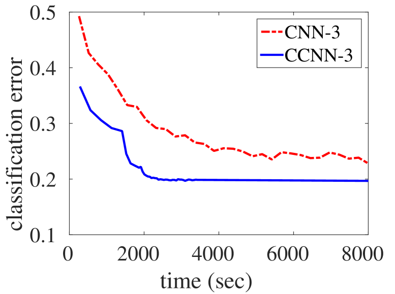
Figure 5: The convergence of CNN-3 and CCNN-3 on the CIFAR-10 dataset.

Results.

We report the classification errors on in Table 5. For models of all depths, the CCNN model outperforms the CNN model. The CCNN-2 and the CCNN-3 model also outperform the three baseline methods. The advantage of the CCNN is substantial for learning two-layer networks, when the optimality guarantee of CCNN holds. The performance improves as more layers are stacked, but as we observe in Table 5, the marginal gain of CCNN diminishes as the network grows deeper. We suspect that this is due to the greedy fashion in which the CCNN layers are constructed. Once trained, the low-level filters of the CCNN are no longer able to adapt to the final classifier. In contrast, the low-level filters of the CNN model are continuously adjusted via backpropagation.

It is worth noting that the performance of the CNN can be further improved by adding more layers, switching from average pooling to max pooling, and being regularized by local response normalization and dropout (see, e.g. [25]). The figures in Table 5 are by no means the state-of-the-art result on CIFAR-10. However, it does demonstrate that the convex relaxation is capable of improving the performance of convolutional neural networks. For future work, we propose to study a better way for convexifying deep CNNs.

In Figure 5, we compare the computational efficiency of CNN-3 to its convexified version CCNN-3. Both models are trained by mini-batch SGD (with batchsize equal to 50) on a single processor. We optimized the choice of step-size for each algorithm. From the plot, it is easy to identify the three stages of the CCNN-3 curve for training the three convolutional layers from bottom to the top. We also observe that the CCNN converges faster than the CNN. More precisely, the CCNN takes half the runtime of the CNN to reach an error rate of 28%, and one-fifth of the runtime to reach an error rate of 23%. The per-iteration cost for training the first layer of CCNN is about 109% of the per-iteration cost of CNN, but the per-iteration cost for training the remaining two layers are about 18% and 7% of that of CNN. Thus, training CCNN scales well to large datasets.

	CNN-1	CNN-2	CNN-3
Original	34.14%	24.98%	21.48%
Convexified	23.62%	21.88%	18.18%

Table 3: Comparing the original CNN and the one whose top convolution layer is convexified by CCNN. The classification errors are reported on CIFAR-10.

Training a CCNN on top of a CNN.

Instead of training a CCNN from scratch, we can also train CCNNs on top of existing CNN layers. More concretely, once a CNN-$k$ model is obtained, we train a two-layer CCNN by taking the $(k-1)$-th hidden layer of CNN as input. This approach preserves the low-level features learned by CNN, only convexifying its top convolutional layer. The underlying motivation is that the traditional CNN is good at learning low-level features through backpropagation, while the CCNN is optimal in learning two-layer networks.

In this experiment, we convexify the top convolutional layer of CNN-2 and CNN-3 using the CCNN approach, with a smaller Gaussian kernel parameter (i.e. $\gamma=0.1$) and keeping other hyperparameters the same as in the training of CCNN-2 and CCNN-3. The results are shown in Table 3. The convexified CNN achieves better accuracy on all network depths. It is worth noting that the time for training a convexified layer is only a small fraction of the time for training the original CNN.

6 Related work

With the empirical success of deep neural networks, there has been an increasing interest in theoretical understanding. Bengio et al. [5] showed how to formulate neural network training as a convex optimization problem involving an infinite number of parameters. This perspective encourages incrementally adding neurons to the network, whose generalization error was studied by Bach [3]. Zhang et al. [47] propose a polynomial-time ensemble method for learning fully-connected neural networks, but their approach handles neither parameter sharing nor the convolutional setting. Other relevant works for learning fully-connected networks include [35, 23, 29]. Aslan et al. [1, 2] propose a method for learning multi-layer latent variable models. They showed that for certain activation functions, the proposed method is a convex relaxation for learning the fully-connected neural network.

Another line of work is devoted to understanding the energy landscape of a neural network. Under certain assumptions on the data distribution, it can be shown that any local minimum of a two-layer fully connected neural network has an objective value that is close to the global minimum value [14, 11]. If this property holds, then gradient descent can find a solution that is “good enough”. Similar results have also been established for over-specified neural networks [34], or neural networks that has a certain parallel topology [20]. However, these results are not applicable to a CNN, since the underlying assumptions are not satisfied by CNNs.

Past work has studied learning translation invariant features without backpropagation. Mairal et al. [30] present convolutional kernel networks. They propose a translation-invariant kernel whose feature mapping can be approximated by a composition of the convolution, non-linearity and pooling operators, obtained through unsupervised learning. However, this method is not equipped with the optimality guarantees that we have provided for CCNNs in this paper, even for learning one convolution layer. The ScatNet method [8] uses translation and deformation-invariant filters constructed by wavelet analysis; however, these filters are independent of the data, unlike the analysis in this paper. Daniely et al. [13] show that a randomly initialized CNN can extract features as powerful as kernel methods, but it is not clear how to provably improve the model from a random initialization.

7 Conclusion

In this paper, we have shown how convex optimization can be used to efficiently optimize CNNs as well as understand them statistically. Our convex relaxation consists of two parts: the nuclear norm relaxation for handling parameter sharing, and the RKHS relaxation for handling non-linearity. For the two-layer CCNN, we proved that its generalization error converges to that of the best possible two-layer CNN. We handled multi-layer CCNNs only heuristically, but observed that adding more layers improves the performance in practice. On real data experiments, we demonstrated that CCNN outperforms the traditional CNN of the same depth, is computationally efficient, and can be combined with the traditional CNN to achieve better performance. A major open problem is to formally study the convex relaxation of deep CNNs.

Acknowledgements

This work was partially supported by Office of Naval Research MURI grant DOD-002888, Air Force Office of Scientific Research Grant AFOSR-FA9550-14-1-001, Office of Naval Research grant ONR-N00014, National Science Foundation Grant CIF-31712-23800, as well as a Microsoft Faculty Research Award to the second author.

Appendix A Inverse polynomial kernel and Gaussian kernel

In this appendix, we describe the properties of the two types of kernels — the inverse polynomial kernel (14) and the Gaussian RBF kernel (15). We prove that the associated reproducing kernel Hilbert Spaces (RKHS) of these kernels contain filters taking the form $h:z\mapsto\sigma(\langle w,z\rangle)$ for particular activation functions $\sigma$.

A.1 Inverse polynomial kernel

We first verify that the function (14) is a kernel function. This holds since that we can find a mapping $\varphi:{\mathbb{R}}^{d_{1}}\to\ell^{2}(\mathbb{N})$ such that $\mathcal{K}(z,z^{\prime})=\langle\varphi(z),\varphi(z^{\prime})\rangle$. We use $z_{i}$ to represent the $i$-th coordinate of an infinite-dimensional vector $z$. The $(k_{1},\dots,k_{j})$-th coordinate of $\varphi(z)$, where $j\in\mathbb{N}$ and $k_{1},\dots,k_{j}\in[d_{1}]$, is defined as $2^{-\frac{j+1}{2}}x_{k_{1}}\dots x_{k_{j}}$. By this definition, we have

$$\langle\varphi(x),\varphi(y)\rangle =\sum_{j=0}^{\infty}2^{-(j+1)}\sum_{(k_{1},\dots,k_{j})\in[d_{1}]^{j}}z_{k_{1}}\dots z_{k_{j}}z^{\prime}_{k_{1}}\dots z^{\prime}_{k_{j}}.$$ (19)

Since $\|{z}\|_{2}\leq 1$ and $\|{z^{\prime}}\|_{2}\leq 1$, the series on the right-hand side is absolutely convergent. The inner term on the right-hand side of equation (19) can be simplified to

$$\sum_{(k_{1},\dots,k_{j})\in[d_{1}]^{j}}z_{k_{1}}\dots z_{k_{j}}z^{\prime}_{k_{1}}\dots z^{\prime}_{k_{j}}=(\langle z,z^{\prime}\rangle)^{j}.$$ (20)

Combining equations (19) and (20) and using the fact that $|\langle z,z^{\prime}\rangle|\leq 1$, we have

$$\langle\varphi(z),\varphi(z^{\prime})\rangle =\sum_{j=0}^{\infty}2^{-(j+1)}(\langle z,z^{\prime}\rangle)^{j}\stackrel{{\scriptstyle\rm(i)}}{{=}}\frac{1}{2-\langle z,z^{\prime}\rangle}=\mathcal{K}(z,z^{\prime}),$$

which verifies that $\mathcal{K}$ is a kernel function and $\varphi$ is the associated feature map. Next, we prove that the associated RKHS contains the class of nonlinear filters. The lemma was proved by Zhang et al. [48]. We include the proof to make the paper self-contained.

Lemma 1.

Assume that the function $\sigma(x)$ has a polynomial expansion $\sigma(t)=\sum_{j=0}^{\infty}a_{j}t^{j}$. Let $C_{\sigma}(\lambda):=\sqrt{\sum_{j=0}^{\infty}2^{j+1}a_{j}^{2}\lambda^{2j}}$. If $C_{\sigma}(\|{w}\|_{2})<\infty$, then the RKHS induced by the inverse polynomial kernel contains function $h:z\mapsto\sigma(\langle w,\,z\rangle)$ with Hilbert norm $\|{h}\|_{\mathcal{H}}=C_{\sigma}(\|{w}\|_{2})$.

Proof.

Let $\varphi$ be the feature map that we have defined for the polynomial inverse kernel. We define vector $\overline{w}\in\ell^{2}(\mathbb{N})$ as follow: the $(k_{1},\dots,k_{j})$-th coordinate of $\overline{w}$, where $j\in\mathbb{N}$ and $k_{1},\dots,k_{j}\in[d_{1}]$, is equal to $2^{\frac{j+1}{2}}a_{j}w_{k_{1}}\dots w_{k_{j}}$. By this definition, we have

$$\sigma(\langle w,z\rangle)=\sum_{t=0}^{\infty}a_{j}(\langle w,z\rangle)^{j}=\sum_{j=0}^{\infty}a_{j}\sum_{(k_{1},\dots,k_{j})\in[d_{1}]^{j}}w_{k_{1}}\dots w_{k_{j}}z_{k_{1}}\dots z_{k_{j}}=\langle\overline{w},\varphi(z)\rangle,$$ (21)

where the first equation holds since $\sigma(x)$ has a polynomial expansion $\sigma(x)=\sum_{j=0}^{\infty}a_{j}x^{j}$, the second by expanding the inner product, and the third by definition of $\overline{w}$ and $\varphi(z)$. The $\ell_{2}$-norm of $\overline{w}$ is equal to:

$$\|{\overline{w}}\|_{2}^{2} =\sum_{j=0}^{\infty}2^{j+1}a_{j}^{2}\sum_{(k_{1},\dots,k_{j})\in[d_{1}]^{j}}\overline{w}_{k_{1}}^{2}\overline{w}_{k_{2}}^{2}\cdots\overline{w}_{k_{j}}^{2}=\sum_{j=0}^{\infty}2^{j+1}a_{j}^{2}\|{\overline{w}}\|_{2}^{2j}=C_{\sigma}^{2}(\|{\overline{w}}\|_{2})<\infty.$$ (22)

By the basic property of the RKHS, the Hilbert norm of $h$ is equal to the $\ell_{2}$-norm of $\overline{w}$. Combining equations (21) and (22), we conclude that $h\in\mathcal{H}$ and $\|{h}\|_{\mathcal{H}}=\|{\overline{w}}\|_{2}=C_{\sigma}(\|{\overline{w}}\|_{2})$. ∎

According to Lemma 1, it suffices to upper bound $C_{\sigma}(\lambda)$ for a particular activation function $\sigma$. To make $C_{\sigma}(\lambda)<\infty$, the coefficients $\{a_{j}\}_{j=0}^{\infty}$ must quickly converge to zero, meaning that the activation function must be sufficiently smooth. For polynomial functions of degree $\ell$, the definition of $C_{\sigma}$ implies that $C_{\sigma}(\lambda)=\mathcal{O}(\lambda^{\ell})$. For the sinusoid activation $\sigma(t):=\sin(t)$, we have

$$C_{\sigma}(\lambda)=\sqrt{\sum_{j=0}^{\infty}\frac{2^{2j+2}}{((2j+1)!)^{2}}\cdot(\lambda^{2})^{2j+1}}\leq 2e^{\lambda^{2}}.$$

For the erf function and the smoothed hinge loss function defined in Section 3.4, Zhang et al. [48, Proposition 1] proved that $C_{\sigma}(\lambda)=\mathcal{O}(e^{c\lambda^{2}})$ for universal numerical constant $c>0$.

A.2 Gaussian kernel

The Gaussian kernel also induces an RKHS that contains a particular class of nonlinear filters. The proof is similar to that of Lemma 1.

Lemma 2.

Assume that the function $\sigma(x)$ has a polynomial expansion $\sigma(t)=\sum_{j=0}^{\infty}a_{j}t^{j}$. Let $C_{\sigma}(\lambda):=\sqrt{\sum_{j=0}^{\infty}\frac{j!e^{2\gamma}}{(2\gamma)^{j}}a_{j}^{2}\lambda^{2j}}$. If $C_{\sigma}(\|{w}\|_{2})<\infty$, then the RKHS induced by the Gaussian kernel contains the function $h:z\mapsto\sigma(\langle w,\,z\rangle)$ with Hilbert norm $\|{h}\|_{\mathcal{H}}=C_{\sigma}(\|{w}\|_{2})$.

Proof.

When $\|{z}\|_{2}=\|{z^{\prime}}\|_{2}=1$, It is well-known [see, e.g. 41] the following mapping $\varphi:{\mathbb{R}}^{d_{1}}\to\ell^{2}(\mathbb{N})$ is a feature map for the Gaussian RBF kernel: the $(k_{1},\dots,k_{j})$-th coordinate of $\varphi(z)$, where $j\in\mathbb{N}$ and $k_{1},\dots,k_{j}\in[d_{1}]$, is defined as $e^{-\gamma}((2\gamma)^{j}/j!)^{1/2}x_{k_{1}}\dots x_{k_{j}}$. Similar to equation (21), we define a vector $\overline{w}\in\ell^{2}(\mathbb{N})$ as follow: the $(k_{1},\dots,k_{j})$-th coordinate of $\overline{w}$, where $j\in\mathbb{N}$ and $k_{1},\dots,k_{j}\in[d_{1}]$, is equal to $e^{\gamma}((2\gamma)^{j}/j!)^{-1/2}a_{j}w_{k_{1}}\dots w_{k_{j}}$. By this definition, we have

$$\sigma(\langle w,z\rangle)=\sum_{t=0}^{\infty}a_{j}(\langle w,z\rangle)^{j}=\sum_{j=0}^{\infty}a_{j}\sum_{(k_{1},\dots,k_{j})\in[d_{1}]^{j}}w_{k_{1}}\dots w_{k_{j}}z_{k_{1}}\dots z_{k_{j}}=\langle\overline{w},\varphi(z)\rangle.$$ (23)

The $\ell_{2}$-norm of $\overline{w}$ is equal to:

$$\|{\overline{w}}\|_{2}^{2} =\sum_{j=0}^{\infty}\frac{j!e^{2\gamma}}{(2\gamma)^{j}}a_{j}^{2}\sum_{(k_{1},\dots,k_{j})\in[d_{1}]^{j}}\overline{w}_{k_{1}}^{2}\overline{w}_{k_{2}}^{2}\cdots\overline{w}_{k_{j}}^{2}=\sum_{j=0}^{\infty}\frac{j!e^{2\gamma}}{(2\gamma)^{j}}a_{j}^{2}\|{\overline{w}}\|_{2}^{2j}=C_{\sigma}^{2}(\|{\overline{w}}\|_{2})<\infty.$$ (24)

Combining equations (21) and (22), we conclude that $h\in\mathcal{H}$ and $\|{h}\|_{\mathcal{H}}=\|{\overline{w}}\|_{2}=C_{\sigma}(\|{\overline{w}}\|_{2})$. ∎

Comparing Lemma 1 and Lemma 2, we find that the Gaussian kernel imposes a stronger condition on the smoothness of the activation function. For polynomial functions of degree $\ell$, we still have $C_{\sigma}(\lambda)=\mathcal{O}(\lambda^{\ell})$. For the sinusoid activation $\sigma(t):=\sin(t)$, it can be verified that

$$C_{\sigma}(\lambda)=\sqrt{e^{2\gamma}\sum_{j=0}^{\infty}\frac{1}{(2j+1)!}\cdot\Big{(}\frac{\lambda^{2}}{2\gamma}\Big{)}^{2j+1}}\leq e^{\lambda^{2}/(4\gamma)+\gamma}.$$

However, the value of $C_{\sigma}(\lambda)$ is infinite when $\sigma$ is the erf function or the smoothed hinge loss, meaning that the Gaussian kernel’s RKHS doesn’t contain filters activated by these two functions.

Appendix B Convex relaxation for nonlinear activation

In this appendix, we provide a detailed derivation of the relaxation for nonlinear activation functions that we previously sketched in Section 3.2. Recall that the filter output is $\sigma(\langle w_{j},\,z\rangle)$. Appendix A shows that given a sufficiently smooth activation function $\sigma$, we can find some kernel function $\mathcal{K}:{\mathbb{R}}^{d_{1}}\times{\mathbb{R}}^{d_{1}}\to{\mathbb{R}}$ and a feature map $\varphi:{\mathbb{R}}^{d_{1}}\to\ell^{2}(\mathbb{N})$ satisfying $\mathcal{K}(z,z^{\prime})\equiv\langle\varphi(z),\,\varphi(z^{\prime})\rangle$, such that

$$\sigma(\langle w_{j},\,z\rangle)\equiv\langle\overline{w}_{j},\,\varphi(z)\rangle.$$ (25)

Here $\overline{w}_{j}\in\ell^{2}(\mathbb{N})$ is a countable-dimensional vector and $\varphi:=(\varphi_{1},\varphi_{2},\dots)$ is a countable sequence of functions. Moreover, the $\ell_{2}$-norm of $\overline{w}_{j}$ is bounded as $\|{\overline{w}_{j}}\|_{2}\leq C_{\sigma}(\|{w_{j}}\|_{2})$ for a monotonically increasing function $C_{\sigma}$ that depends on the kernel (see Lemma 1 and Lemma 2). As a consequence, we may use $\varphi(z)$ as the vectorized representation of the patch $z$, and use $\overline{w}_{j}$ as the linear transformation weights, then the problem is reduced to training a CNN with the identity activation function.

The filter is parametrized by an infinite-dimensional vector $\overline{w}_{j}$. Our next step is to reduce the original ERM problem to a finite-dimensional one. In order to minimize the empirical risk, one only needs to concern the output on the training data, that is, the output of $\langle\overline{w}_{j},\,\varphi(z_{p}(x_{i}))\rangle$ for all $(i,p)\in[n]\times[P]$. Let $T$ be the orthogonal projector onto the linear subspace spanned by the vectors $\{\varphi(z_{p}(x_{i})):(i,p)\in[n]\times[P]\}$. Then we have

$$\forall~{}(i,p)\in[n]\times[P]:\quad\langle\overline{w}_{j},\,\varphi(z_{p}(x_{i}))\rangle=\langle\overline{w}_{j},\,T\varphi(z_{p}(x_{i}))\rangle=\langle T\overline{w}_{j},\,\varphi(z_{p}(x_{i}))\rangle.$$

The last equation follows since the orthogonal projector $T$ is self-adjoint. Thus, for empirical risk minimization, we can without loss of generality assume that $\overline{w}_{j}$ belongs to the linear subspace spanned by $\{\varphi(z_{p}(x_{i})):(i,p)\in[n]\times[P]\}$ and reparametrize it by:

$$\overline{w}_{j}=\sum_{(i,p)\in[n]\times[P]}\beta_{j,(i,p)}\varphi(z_{p}(x_{i})).$$ (26)

Let $\beta_{j}\in{\mathbb{R}}^{nP}$ be a vector whose whose $(i,p)$-th coordinate is $\beta_{j,(i,p)}$. In order to estimate $\overline{w}_{j}$, it suffices to estimate the vector $\beta_{j}$. By definition, the vector satisfies the relation $\beta_{j}^{\top}K\beta_{j}=\|{\overline{w}_{j}}\|_{2}^{2}$, where $K$ is the $nP\times nP$ kernel matrix defined in Section 3.2. As a consequence, if we can find a matrix $Q$ such that $QQ^{\top}=K$, then we have the norm constraint

$$\|{Q^{\top}\beta_{j}}\|_{2}=\sqrt{\beta_{j}^{\top}K\beta_{j}}=\|{\overline{w}_{j}}\|_{2}\leq C_{\sigma}(\|{w_{j}}\|_{2})\leq C_{\sigma}(B).$$ (27)

Let $v(z)\in\mathbb{R}^{nP}$ be a vector whose $(i,p)$-th coordinate is equal to $\mathcal{K}(z,z_{p}(x_{i}))$. Then by equations (25) and (26), the filter output can be written as

$$\sigma\big{(}\langle w_{j},\,z\rangle\big{)} \equiv\langle\overline{w}_{j},\,\varphi(z)\rangle\,\equiv\,\langle\beta_{j},\,v(z)\rangle.$$ (28)

For any patch $z_{p}(x_{i})$ in the training data, the vector $v(z_{p}(x_{i}))$ belongs to the column space of the kernel matrix $K$. Therefore, letting $Q^{\dagger}$ represent the pseudo-inverse of matrix $Q$, we have

$$\forall~{}(i,p)\in[n]\times[P]:\quad\langle\beta_{j},\,v(z_{p}(x_{i}))\rangle=\beta_{j}^{\top}QQ^{\dagger}v(z_{p}(x_{i}))=\langle(Q^{\top})^{\dagger}Q^{\top}\beta_{j},\,v(z_{p}(x_{i}))\rangle.$$

It means that if we replace the vector $\beta_{j}$ on the right-hand side of equation (28) by the vector $(Q^{\top})^{\dagger}Q^{\top}\beta_{j}$, then it won’t change the empirical risk. Thus, for ERM we can parametrize the filters by

$$h_{j}(z):=\langle(Q^{\top})^{\dagger}Q^{\top}\beta_{j},\,v(z)\rangle=\langle Q^{\dagger}v(z),\,Q^{\top}\beta_{j}\rangle.$$ (29)

Let $Z(x)$ be an $P\times nP$ matrix whose $p$-th row is equal to $Q^{\dagger}v(z_{p}(x))$. Similar to the steps in equation (6), we have

$$f_{k}(x)=\sum_{j=1}^{r}\alpha_{k,j}^{\top}Z(x)K^{1/2}\beta_{j}={\rm tr}\Big{(}Z(x)\Big{(}\sum_{j=1}^{r}K^{1/2}\beta_{j}\alpha_{k,j}^{\top}\Big{)}\Big{)}={\rm tr}(Z(x)A_{k}),$$

where $A_{k}:=\sum_{j=1}^{r}Q^{\top}\beta_{j}\alpha_{k,j}^{\top}$. If we let $A:=(A_{1},\dots,A_{d_{2}})$ denote the concatenation of these matrices, then this larger matrix satisfies the constraints:

Constraint (C1):

$\max\limits_{j\in[r]}\|{Q^{\top}\beta_{j}}\|_{2}\leq C_{\sigma}(B_{1})$ and $\max\limits_{(k,j)\in[d_{2}]\times[r]}\|{\alpha_{k,j}}\|_{2}\leq B_{2}$.

Constraint (C2):

The matrix $A$ has rank at most $r$.

We relax these two constraints to the nuclear norm constraint:

$$\|{A}\|_{*}\leq C_{\sigma}(B_{1})B_{2}r\sqrt{d_{2}}.$$ (30)

By comparing constraints (8) and (30), we see that the only difference is that the term $B_{1}$ in the norm bound has been replaced by $C_{\sigma}(B_{1})$. This change is needed because we have used the kernel trick to handle nonlinear activation functions.

Appendix C Proof of Theorem 1

Since the output is one-dimensional in this case, we can adopt the simplified notation $(A,\alpha_{j,p})$ for the matrix $(A_{1},\alpha_{1,j,p})$. Letting $\mathcal{H}$ be the RKHS associated with the kernel function $\mathcal{K}$, and letting $\|{\cdot}\|_{\mathcal{H}}$ be the associated Hilbert norm, consider the function class

$$\mathcal{F}_{\text{ccnn}}:=\Big{\{}x\mapsto\sum_{j=1}^{r^{*}}\sum_{p=1}^{P}\alpha_{j,p}h_{j}(z_{p}(x)):\;r^{*}<\infty\mbox{ and }\sum_{j=1}^{r^{*}}\|{\alpha_{j}}\|_{2}\|{h_{j}}\|_{\mathcal{H}}\leq C_{\sigma}(B_{1})B_{2}d_{2}\Big{\}}.$$ (31)

Here $\alpha_{j,p}$ denotes the $p$-th entry of vector $\alpha_{j}\in{\mathbb{R}}^{P}$, whereas the quantity $C_{\sigma}(B_{1})$ only depends on $B_{1}$ and the activation function $\sigma$. The following lemma shows that the function class $\mathcal{F}_{\text{ccnn}}$ is rich enough so that it contains family of CNN predictors as a subset. The reader should recall the notion of a valid activation function, as defined prior to the statement of Theorem 1.

Lemma 3.

For any valid activation function $\sigma$, there is a quantity $C_{\sigma}(B_{1})$, depending only on $B_{1}$ and $\sigma$, such that $\mathcal{F}_{\text{cnn}}\subset\mathcal{F}_{\text{ccnn}}$.

See Appendix C.1 for the proof.

Next, we connect the function class $\mathcal{F}_{\text{ccnn}}$ to the CCNN algorithm. Recall that $\widehat{f}_{\text{ccnn}}$ is the predictor trained by the CCNN algorithm. The following lemma shows that $\widehat{f}_{\text{ccnn}}$ is an empirical risk minimizer within $\mathcal{F}_{\text{ccnn}}$.

Lemma 4.

With the CCNN hyper-parameter $R=C_{\sigma}(B_{1})B_{2}d_{2}$, the predictor $\widehat{f}_{\text{ccnn}}$ is guaranteed to satisfy the inclusion

$$\widehat{f}_{\text{ccnn}}\in\arg\min_{f\in\mathcal{F}_{\text{ccnn}}}\sum_{i=1}^{n}\mathcal{L}(f(x_{i});y_{i}).$$

See Appendix C.2 for the proof.

Our third lemma shows that the function class $\mathcal{F}_{\text{ccnn}}$ is not “too big”, which we do by upper bounding its Rademacher complexity. The Rademacher complexity of a function class $\mathcal{F}=\{f:\mathcal{X}\to{\mathbb{R}}\}$ with respect to $n$ i.i.d. samples $\{X_{i}\}_{i=1}^{n}$ is given by

$${\mathcal{R}}_{n}(\mathcal{F}):=\mathbb{E}_{X,\epsilon}\left[\sup_{f\in\mathcal{F}}\frac{1}{n}\sum_{i=1}^{n}\epsilon_{i}f(X_{i})\right],$$

where $\{\epsilon_{i}\}_{i=1}^{n}$ are an i.i.d. sequence of uniform $\{-1,+1\}$-valued variables. Rademacher complexity plays an important role in empirical process theory, and in particular can be used to bound the generalization loss of our empirical risk minimization problem. We refer the reader to Bartlett and Mendelson [4] for an introduction to the theoretical properties of Rademacher complexity.

The following lemma involves the kernel matrix $K(x)\in{\mathbb{R}}^{P\times P}$ whose $(i,j)$-th entry is equal to $\mathcal{K}(z_{i}(x),z_{j}(x))$, as well as the expectation $\mathbb{E}[\|{K(X)}\|_{2}]$ of the spectral norm of this matrix when $X$ is drawn randomly.

Lemma 5.

There is a universal constant $c$ such that

$${\mathcal{R}}_{n}(\mathcal{F}_{\text{ccnn}})\leq\frac{c\;C_{\sigma}(B_{1})B_{2}r\sqrt{\log(nP)\mathbb{E}[\|{K(X)}\|_{2}]}}{\sqrt{n}}.$$ (32)

See Appendix C.3 for the proof of this claim.

Combining Lemmas 3 through 5 allows us to compare the CCNN predictor $\widehat{f}_{\text{ccnn}}$ against the best model in the CNN class. Lemma 4 shows that $\widehat{f}_{\text{ccnn}}$ is the empirical risk minimizer within function class $\mathcal{F}_{\text{ccnn}}$. Thus, the theory of Rademacher complexity [4] guarantees that

$$\mathbb{E}[\mathcal{L}(\mathcal{F}_{\text{ccnn}}(X);Y)]\leq\inf_{f\in\mathcal{F}_{\text{ccnn}}}\mathbb{E}[\mathcal{L}(f(x);y)]+2L\cdot{\mathcal{R}}_{n}(\mathcal{F}_{\text{ccnn}})+\frac{c}{\sqrt{n}},$$ (33)

where $c$ is a universal constant. By Lemma 3, we have

$$\inf_{f\in\mathcal{F}_{\text{ccnn}}}\mathbb{E}[\mathcal{L}(f(X);Y)]\leq\inf_{f\in\mathcal{F}_{\text{cnn}}}\mathbb{E}[\mathcal{L}(f(X);Y)].$$

Plugging this upper bound into inequality (33) and applying Lemma 5 completes the proof.

C.1 Proof of Lemma 3

With the activation functions specified in the lemma statement, Lemma 1 and Lemma 2 show that there is a quantity $C_{\sigma}(B_{1})$, such any filter of CNN belongs to the reproducing kernel Hilbert space $\mathcal{H}$ and its Hilbert norm is bounded by $C_{\sigma}(B_{1})$. As a consequence, any function $f\in\mathcal{F}_{\text{cnn}}$ can be represented by

$$f(x):=\sum_{j=1}^{r}\sum_{p=1}^{P}\alpha_{j,p}h_{j}(z_{p}(x))\quad\mbox{where $\|{h_{j}}\|_{\mathcal{H}}\leq C_{\sigma}(B_{1})$ and $\|{\alpha_{j}}\|_{2}\leq B_{2}$}.$$

It is straightforward to verify that function $f$ satisfies the constraint in equation (31), and consequently belongs to $\mathcal{F}_{\text{ccnn}}$.

C.2 Proof of Lemma 4

Let $\mathcal{C}_{R}$ denote the function class $\big{\{}x\mapsto{\rm tr}(Z(x)A):\;\|{A}\|_{*}\leq R\big{\}}$. We first prove that $\mathcal{C}_{R}\subset\mathcal{F}_{\text{ccnn}}$. Consider an arbitrary function $f_{A}(x):\,={\rm tr}(Z(x)A)$ belonging to $\mathcal{C}_{R}$. Note that the matrix $A$ has a singular value decomposition (SVD) $A=\sum_{j=1}^{r^{*}}\lambda_{j}w_{j}u_{j}^{\top}$ for some ${r^{*}}<\infty$, where $w_{j}$ and $u_{j}$ are unit vectors and $\lambda_{j}$ are real numbers. Using this notation, the function $f_{A}$ can be represented as the sum

$$f_{A}(x)=\sum_{j=1}^{r^{*}}\lambda_{j}u_{j}^{\top}Z(x)w_{j}.$$

Let $v(z)$ be an $nP$-dimensional vector whose $(i,p)$-th coordinate is equal to $\mathcal{K}(z,z_{p}(x_{i}))$. Then $Q^{\dagger}v(z_{p}(x))$ is the $p$-th row of matrix $Z(x)$. Letting $h_{j}$ denote the mapping $z\mapsto\langle Q^{\dagger}v(z),w_{j}\rangle$, we have

$$f_{A}(x)=\sum_{j=1}^{r^{*}}\sum_{p=1}^{P}\lambda_{j}u_{j,p}h_{j}(z_{p}(x)).$$

The function $h_{j}$ can also be written as $z\mapsto\langle(Q^{\top})^{\dagger}w_{j},v(z)\rangle$. Equation (27) implies that the Hilbert norm of this function is equal to $\|{Q^{\top}(Q^{\top})^{\dagger}w_{j}}\|_{2}$, which is bounded by $\|{w_{j}}\|_{2}=1$. Thus we have

$$\sum_{j=1}^{r^{*}}\|{\lambda_{j}u_{j}}\|_{2}\|{h_{j}}\|_{\mathcal{H}}=\sum_{j=1}^{r^{*}}|\lambda_{j}|=\|{A}\|_{*}\leq C_{\sigma}(B_{1})B_{2}r,$$

which implies that $f_{A}\in\mathcal{F}_{\text{ccnn}}$.

Next, it suffices to prove that for some empirical risk minimizer $f$ in function class $\mathcal{F}_{\text{ccnn}}$, it also belongs to the function class $\mathcal{C}_{R}$. Recall that any function $f\in\mathcal{F}_{\text{ccnn}}$ can be represented in the form

$$f(x)=\sum_{j=1}^{r^{*}}\sum_{p=1}^{P}\alpha_{j,p}h_{j}(z_{p}(x)).$$

where the filter $h_{j}$ belongs to the RKHS. Let $\varphi:{\mathbb{R}}^{d_{1}}\to\ell^{2}(\mathbb{N})$ be a feature map of the kernel function. The function $h_{j}(z)$ can be represented by $\langle\overline{w},\,\varphi(z)\rangle$ for some $\overline{w}\in\ell^{2}(\mathbb{N})$. In Appendix B, we have shown that any function taking this form can be replaced by $\langle(Q^{\top})^{\dagger}Q^{\top}\beta_{j},\,v(z)\rangle$ for some vector $\beta_{j}\in{\mathbb{R}}^{nP}$ without changing the output on the training data. Thus, there exists at least one empirical risk minimizer $f$ of $\mathcal{F}_{\text{ccnn}}$ such that all of its filters take the form

$$h_{j}(z)=\langle(Q^{\top})^{\dagger}Q^{\top}\beta_{j},\,v(z)\rangle.$$ (34)

By equation (27), the Hilbert norm of these filters satisfy:

$$\|{h_{j}}\|_{\mathcal{H}}=\|{Q^{\top}(Q^{\top})^{\dagger}Q^{\top}\beta_{j}}\|_{2}=\|{Q^{\top}\beta_{j}}\|_{2}.$$

According to Appendix B, if all filters take the form (34), then the function $f$ can be represented by ${\rm tr}(Z(x)A)$ for matrix $A:=\sum_{j=1}^{r^{*}}Q^{\top}\beta_{j}\alpha_{j}^{\top}$. Consequently, the nuclear norm is bounded as

$$\|{A}\|_{*}\leq\sum_{j=1}^{r^{*}}\|{\alpha_{j}}\|_{2}\|{Q^{\top}\beta_{j}}\|_{2}=\sum_{j=1}^{r^{*}}\|{\alpha_{j}}\|_{2}\|{h_{j}}\|_{\mathcal{H}}\leq C_{\sigma}(B_{1})B_{2}r=R,$$

which establishes that the function $f$ belongs to the function class $\mathcal{C}_{R}$.

C.3 Proof of Lemma 5

Throughout this proof, we use the shorthand notation $R:=C_{\sigma}(B_{1})B_{2}r$. Recall that any function $f\in\mathcal{F}_{\text{ccnn}}$ can be represented in the form

$$f(x)=\sum_{j=1}^{r^{*}}\sum_{p=1}^{P}\alpha_{j,p}h_{j}(z_{p}(x))\quad\mbox{where $h_{j}\in\mathcal{H}$},$$ (35)

and the Hilbert space $\mathcal{H}$ is induced by the kernel function $\mathcal{K}$. Since any patch $z$ belongs to the compact space $\{z:\|{z}\|_{2}\leq 1\}$ and $\mathcal{K}$ is a continuous kernel satisfying $\mathcal{K}(z,z)\leq 1$, Mercer’s theorem [41, Theorem 4.49] implies that there is a feature map $\varphi:{\mathbb{R}}^{d_{1}}\to\ell^{2}(\mathbb{N})$ such that $\sum_{\ell=1}^{\infty}\varphi_{\ell}(z)\varphi_{\ell}(z^{\prime})$ converges uniformly and absolutely to $\mathcal{K}(z,z^{\prime})$. Thus, we can write $\mathcal{K}(z,z^{\prime})=\langle\varphi(z),\,\varphi(z^{\prime})\rangle$. Since $\varphi$ is a feature map, every any function $h\in\mathcal{H}$ can be written as $h(z)=\langle\beta,\,\varphi(z)\rangle$ for some $\beta\in\ell^{2}(\mathbb{N})$, and the Hilbert norm of $h$ is equal to $\|{\beta}\|_{2}$.

Using this notation, we can write the filter $h_{j}$ in equation (35) as $h_{j}(z)=\langle\beta_{j},\varphi(z)\rangle$ for some vector $\beta_{j}\in\ell^{2}(\mathbb{N})$, with Hilbert norm $\|{h_{j}}\|_{\mathcal{H}}=\|{\beta_{j}}\|_{2}$. For each $x$, let $\Psi(x)$ denote the linear operator that maps any sequence $\theta\in\ell^{2}(\mathbb{N})$ to the vector in $\mathbb{R}^{P}$ with elements

$$\begin{bmatrix}\langle\theta,\,\varphi(z_{1}(x))\rangle&\ldots&\langle\theta,\,\varphi(z_{P}(x))\rangle\end{bmatrix}^{T}.$$

Informally, we can think of $\Psi(x)$ as a matrix whose $p$-th row is equal to $\varphi(z_{p}(x))$. The function $f$ can then be written as

$$f(x_{i})=\sum_{j=1}^{{r^{*}}}\alpha_{j}^{\top}\Psi(x_{i})\beta_{j}={\rm tr}\left(\Psi(x_{i})\Big{(}\sum_{j=1}^{{r^{*}}}\beta_{j}\alpha_{j}^{\top}\Big{)}\right).$$ (36)

The matrix $\sum_{j=1}^{{r^{*}}}\beta_{j}\alpha_{j}^{\top}$ satisfies the constraint

$$\left\|{\sum_{j=1}^{{r^{*}}}\beta_{j}\alpha_{j}^{\top}}\right\|_{*}\leq\sum_{j=1}^{r^{*}}\|{\alpha_{j}}\|_{2}\cdot\|{\beta_{j}}\|_{2}=\sum_{j=1}^{r^{*}}\|{\alpha_{j}}\|_{2}\cdot\|{h_{j}}\|_{\mathcal{H}}\leq R.$$ (37)

Combining equation (36) and inequality (37), we find that the Rademacher complexity is bounded by

$$R_{n}(\mathcal{F}_{\text{ccnn}})=\frac{1}{n}\mathbb{E}\left[\sup_{f\in\mathcal{F}_{\text{ccnn}}}\sum_{i=1}^{n}\epsilon_{i}f(x_{i})\right] \leq\frac{1}{n}\mathbb{E}\left[\sup_{A:\|{A}\|_{*}\leq R}{\rm tr}\left(\Big{(}\sum_{i=1}^{n}\epsilon_{i}\Psi(x_{i})\Big{)}A\right)\right]$$

$$=\frac{R}{n}\mathbb{E}\left[\left\|{\sum_{i=1}^{n}\epsilon_{i}\Psi(x_{i})}\right\|_{2}\right],$$ (38)

where the last equality uses Hölder’s inequality—that is, the duality between the nuclear norm and the spectral norm.

As noted previously, we may think informally of the quantity $\sum_{i=1}^{n}\epsilon_{i}\Psi(x_{i})$ as a matrix with $P$ rows and infinitely many columns. Let $\Psi^{(d)}(x_{i})$ denote the submatrix consisting of the first $d$ columns of $\Psi(x_{i})$ and let $\Psi^{(-d)}(x_{i})$ denote the remaining sub-matrix. We have

$$\mathbb{E}\left[\left\|{\sum_{i=1}^{n}\epsilon_{i}\Psi(x_{i})}\right\|_{2}\right] \leq\mathbb{E}\left[\left\|{\sum_{i=1}^{n}\epsilon_{i}\Psi^{(d)}(x_{i})}\right\|_{2}\right]+\left(\mathbb{E}\left[\left\|{\sum_{i=1}^{n}\epsilon_{i}\Psi^{(-d)}(x_{i})}\right\|_{F}^{2}\right]\right)^{1/2}$$

$$\leq\mathbb{E}\left[\left\|{\sum_{i=1}^{n}\epsilon_{i}\Psi^{(d)}(x_{i})}\right\|_{2}\right]+\left(nP\cdot\mathbb{E}\left[\sum_{\ell=d+1}^{\infty}\varphi^{2}_{\ell}(z)\right]\right)^{1/2}.$$

Since $\sum_{\ell=1}^{\infty}\varphi^{2}_{\ell}(z)$ uniformly converges to $\mathcal{K}(z,z)$, the second term on the right-hand side converges to zero as $d\to\infty$. Thus it suffices to bound the first term and take the limit. In order to upper bound the spectral norm $\left\|{\sum_{i=1}^{n}\epsilon_{i}\Psi^{(d)}(x_{i})}\right\|_{2}$, we use a matrix Bernstein inequality due to Minsker [31, Theorem 2.1]. In particular, whenever ${\rm tr}(\Psi^{(d)}(x_{i})(\Psi^{(d)}(x_{i}))^{\top})\leq C_{1}$, there is a universal constant $c$ such that the expected spectral norm is upper bounded as

$$\mathbb{E}\left[\left\|{\sum_{i=1}^{n}\epsilon_{i}\Psi^{(d)}(x_{i})}\right\|_{2}\right] \leq c\;\sqrt{\log(nC_{1})}\mathbb{E}\Big{[}\Big{(}\sum_{i=1}^{n}\|{\Psi^{(d)}(x_{i})(\Psi^{(d)}(x_{i}))^{\top}}\|_{2}\Big{)}^{1/2}\Big{]}$$

$$\leq c\;\sqrt{\log(nC_{1})}\Big{(}n\mathbb{E}[\|{\Psi(X)\Psi^{\top}(X)}\|_{2}]\Big{)}^{1/2}.$$

Note that the uniform kernel expansion $\mathcal{K}(z,z^{\prime})=\sum_{\ell=1}^{\infty}\varphi_{\ell}(z)\varphi_{\ell}(z^{\prime})$ implies the trace norm bound ${\rm tr}(\Psi^{(d)}(x_{i})(\Psi^{(d)}(x_{i}))^{\top})\leq{\rm tr}(K(x_{i}))$. Since all patches are contained in the unit $\ell_{2}$-ball, the kernel function $\mathcal{K}$ is uniformly bounded by $1$, and hence $C_{1}\leq P$. Taking the limit $d\to\infty$, we find that

$$\mathbb{E}\left[\left\|{\sum_{i=1}^{n}\epsilon_{i}\Psi(x_{i})}\right\|_{2}\right]\leq c\;\sqrt{\log(nP)}\Big{(}n\mathbb{E}[\|{K(X)}\|_{2}]\Big{)}^{1/2}.$$

Finally, substituting this upper bound into inequality (C.3) yields the claimed bound (32).

References

- Aslan et al. [2013] Ö. Aslan, H. Cheng, X. Zhang, and D. Schuurmans. Convex two-layer modeling. In Advances in Neural Information Processing Systems, pages 2985–2993, 2013.
- Aslan et al. [2014] Ö. Aslan, X. Zhang, and D. Schuurmans. Convex deep learning via normalized kernels. In Advances in Neural Information Processing Systems, pages 3275–3283, 2014.
- Bach [2014] F. Bach. Breaking the curse of dimensionality with convex neural networks. arXiv preprint arXiv:1412.8690, 2014.
- Bartlett and Mendelson [2003] P. L. Bartlett and S. Mendelson. Rademacher and Gaussian complexities: Risk bounds and structural results. The Journal of Machine Learning Research, 3:463–482, 2003.
- Bengio et al. [2005] Y. Bengio, N. L. Roux, P. Vincent, O. Delalleau, and P. Marcotte. Convex neural networks. In Advances in Neural Information Processing Systems, pages 123–130, 2005.
- Blum and Rivest [1992] A. L. Blum and R. L. Rivest. Training a 3-node neural network is NP-complete. Neural Networks, 5(1):117–127, 1992.
- Bottou [1998] L. Bottou. Online learning and stochastic approximations. On-line learning in neural networks, 17(9):142, 1998.
- Bruna and Mallat [2013] J. Bruna and S. Mallat. Invariant scattering convolution networks. Pattern Analysis and Machine Intelligence, IEEE Transactions on, 35(8):1872–1886, 2013.
- Chan et al. [2015] T.-H. Chan, K. Jia, S. Gao, J. Lu, Z. Zeng, and Y. Ma. Pcanet: A simple deep learning baseline for image classification? IEEE Transactions on Image Processing, 24(12):5017–5032, 2015.
- Chen and Manning [2014] D. Chen and C. D. Manning. A fast and accurate dependency parser using neural networks. In Proceedings of the 2014 Conference on Empirical Methods in Natural Language Processing (EMNLP), volume 1, pages 740–750, 2014.
- Choromanska et al. [2014] A. Choromanska, M. Henaff, M. Mathieu, G. B. Arous, and Y. LeCun. The loss surface of multilayer networks. ArXiv:1412.0233, 2014.
- Coates et al. [2010] A. Coates, H. Lee, and A. Y. Ng. An analysis of single-layer networks in unsupervised feature learning. Ann Arbor, 1001(48109):2, 2010.
- Daniely et al. [2016] A. Daniely, R. Frostig, and Y. Singer. Toward deeper understanding of neural networks: The power of initialization and a dual view on expressivity. arXiv preprint arXiv:1602.05897, 2016.
- Dauphin et al. [2014] Y. N. Dauphin, R. Pascanu, C. Gulcehre, K. Cho, S. Ganguli, and Y. Bengio. Identifying and attacking the saddle point problem in high-dimensional non-convex optimization. In Advances in Neural Information Processing Systems, pages 2933–2941, 2014.
- Drineas and Mahoney [2005] P. Drineas and M. W. Mahoney. On the Nyström method for approximating a Gram matrix for improved kernel-based learning. The Journal of Machine Learning Research, 6:2153–2175, 2005.
- Duchi et al. [2008] J. Duchi, S. Shalev-Shwartz, Y. Singer, and T. Chandra. Efficient projections onto the -ball for learning in high dimensions. In Proceedings of the 25th International Conference on Machine Learning, pages 272–279. ACM, 2008.
- Duchi et al. [2011] J. Duchi, E. Hazan, and Y. Singer. Adaptive subgradient methods for online learning and stochastic optimization. The Journal of Machine Learning Research, 12:2121–2159, 2011.
- Eldar and Kutyniok [2012] Y. C. Eldar and G. Kutyniok. Compressed sensing: theory and applications. Cambridge University Press, 2012.
- Fahlman [1988] S. E. Fahlman. An empirical study of learning speed in back-propagation networks. Journal of Heuristics, 1988.
- Haeffele and Vidal [2015] B. D. Haeffele and R. Vidal. Global optimality in tensor factorization, deep learning, and beyond. arXiv preprint arXiv:1506.07540, 2015.
- Hinton et al. [2012] G. Hinton, L. Deng, D. Yu, G. E. Dahl, A.-r. Mohamed, N. Jaitly, A. Senior, V. Vanhoucke, P. Nguyen, T. N. Sainath, et al. Deep neural networks for acoustic modeling in speech recognition: The shared views of four research groups. Signal Processing Magazine, IEEE, 29(6):82–97, 2012.
- Isa et al. [2010] I. Isa, Z. Saad, S. Omar, M. Osman, K. Ahmad, and H. M. Sakim. Suitable mlp network activation functions for breast cancer and thyroid disease detection. In 2010 Second International Conference on Computational Intelligence, Modelling and Simulation, pages 39–44, 2010.
- Janzamin et al. [2015] M. Janzamin, H. Sedghi, and A. Anandkumar. Generalization bounds for neural networks through tensor factorization. ArXiv:1506.08473, 2015.
- Krizhevsky and Hinton [2009] A. Krizhevsky and G. Hinton. Learning multiple layers of features from tiny images. Master Thesis, 2009.
- Krizhevsky et al. [2012] A. Krizhevsky, I. Sutskever, and G. E. Hinton. Imagenet classification with deep convolutional neural networks. In Advances in Neural Information Processing Systems, pages 1097–1105, 2012.
- Lawrence et al. [1997] S. Lawrence, C. L. Giles, A. C. Tsoi, and A. D. Back. Face recognition: A convolutional neural-network approach. Neural Networks, IEEE Transactions on, 8(1):98–113, 1997.
- Le et al. [2013] Q. Le, T. Sarlós, and A. Smola. Fastfood-approximating kernel expansions in loglinear time. In Proceedings of the International Conference on Machine Learning, 2013.
- LeCun et al. [1998] Y. LeCun, L. Bottou, Y. Bengio, and P. Haffner. Gradient-based learning applied to document recognition. Proceedings of the IEEE, 86(11):2278–2324, 1998.
- Livni et al. [2014] R. Livni, S. Shalev-Shwartz, and O. Shamir. On the computational efficiency of training neural networks. In Advances in Neural Information Processing Systems, pages 855–863, 2014.
- Mairal et al. [2014] J. Mairal, P. Koniusz, Z. Harchaoui, and C. Schmid. Convolutional kernel networks. In Advances in Neural Information Processing Systems, pages 2627–2635, 2014.
- Minsker [2011] S. Minsker. On some extensions of Bernstein’s inequality for self-adjoint operators. arXiv preprint arXiv:1112.5448, 2011.
- Mnih et al. [2015] V. Mnih, K. Kavukcuoglu, D. Silver, A. A. Rusu, J. Veness, M. G. Bellemare, A. Graves, M. Riedmiller, A. K. Fidjeland, G. Ostrovski, et al. Human-level control through deep reinforcement learning. Nature, 518(7540):529–533, 2015.
- Rahimi and Recht [2007] A. Rahimi and B. Recht. Random features for large-scale kernel machines. In Advances in Neural Information Processing Systems, pages 1177–1184, 2007.
- Safran and Shamir [2015] I. Safran and O. Shamir. On the quality of the initial basin in overspecified neural networks. arXiv preprint arXiv:1511.04210, 2015.
- Sedghi and Anandkumar [2014] H. Sedghi and A. Anandkumar. Provable methods for training neural networks with sparse connectivity. ArXiv:1412.2693, 2014.
- Shalev-Shwartz et al. [2011] S. Shalev-Shwartz, O. Shamir, and K. Sridharan. Learning kernel-based halfspaces with the 0-1 loss. SIAM Journal on Computing, 40(6):1623–1646, 2011.
- Silver et al. [2016] D. Silver, A. Huang, C. J. Maddison, A. Guez, L. Sifre, G. Van Den Driessche, J. Schrittwieser, I. Antonoglou, V. Panneershelvam, M. Lanctot, et al. Mastering the game of Go with deep neural networks and tree search. Nature, 529(7587):484–489, 2016.
- Sohn and Lee [2012] K. Sohn and H. Lee. Learning invariant representations with local transformations. In Proceedings of the 29th International Conference on Machine Learning (ICML-12), pages 1311–1318, 2012.
- Sopena et al. [1999] J. M. Sopena, E. Romero, and R. Alquezar. Neural networks with periodic and monotonic activation functions: a comparative study in classification problems. In ICANN 99, pages 323–328, 1999.
- Srivastava et al. [2014] N. Srivastava, G. Hinton, A. Krizhevsky, I. Sutskever, and R. Salakhutdinov. Dropout: A simple way to prevent neural networks from overfitting. The Journal of Machine Learning Research, 15(1):1929–1958, 2014.
- Steinwart and Christmann [2008] I. Steinwart and A. Christmann. Support vector machines. Springer, New York, 2008.
- Tang [2013] Y. Tang. Deep learning using linear support vector machines. arXiv preprint arXiv:1306.0239, 2013.
- [43] VariationsMNIST. Variations on the MNIST digits. http://www.iro.umontreal.ca/~lisa/twiki/bin/view.cgi/Public/MnistVariations, 2007.
- Vincent et al. [2010] P. Vincent, H. Larochelle, I. Lajoie, Y. Bengio, and P.-A. Manzagol. Stacked denoising autoencoders: Learning useful representations in a deep network with a local denoising criterion. The Journal of Machine Learning Research, 11:3371–3408, 2010.
- Wang et al. [2012] T. Wang, D. J. Wu, A. Coates, and A. Y. Ng. End-to-end text recognition with convolutional neural networks. In Pattern Recognition (ICPR), 2012 21st International Conference on, pages 3304–3308. IEEE, 2012.
- Xiao and Zhang [2014] L. Xiao and T. Zhang. A proximal stochastic gradient method with progressive variance reduction. SIAM Journal on Optimization, 24(4):2057–2075, 2014.
- Zhang et al. [2015] Y. Zhang, J. D. Lee, M. J. Wainwright, and M. I. Jordan. Learning halfspaces and neural networks with random initialization. arXiv preprint arXiv:1511.07948, 2015.
- Zhang et al. [2016] Y. Zhang, J. D. Lee, and M. I. Jordan. -regularized neural networks are improperly learnable in polynomial time. In Proceedings on the 33rd International Conference on Machine Learning, 2016.