High performance volume ray casting:
A branchless generalized Joseph projector

Abstract

A concise and highly performant branchless formulation of a Joseph-type interpolating ray-casting algorithm for the computation of X-ray projections is presented. It efficiently utilizes the hardware resources of modern graphics processing units at the scale of their theoretic maximum performance reaching access rates of 600 GB/s within read-and-write memory, and is further shown to do so without compromising on image quality. The computation of X-ray projections from discrete voxel grids is an ubiquitous task in many problems related to volume image processing, including tomographic reconstruction and visualization. Although its central role has given rise to numerous publications discussing the optimal modeling of ray-volume intersections, a unique benchmark in this respect does not exist. Here, a 3D Shepp-Logan phantom is used, which allows the computation of analytic reference projections that can further serve as input to iterative reconstructions without committing the inverse crime. The proposed algorithm (GJP) is compared to the competing and widely adopted digital differential analyzer (DDA), which computes exact line-box intersections. It is thereby found to outperform the DDA on recent graphics processors in all respects: Despite accessing twice as much memory, the GJP is still able to calculate projections twice as fast. It further exhibits considerably less discretization artifacts, and neither oversampling of the DDA nor a smooth interpolation kernel within the GJP are able to improve on these results in any respect.

I Introduction

The simulation of X-ray images (or the generation of “digitally reconstructed radiographs”) by numeric projection of gridded volume images represents, in the context of computed tomography, the calculation of the forward problem within iterative solutions of the inverse problem, i.e., the reconstruction problem. It is thus also referred to as “forward projection” (as opposed to the “backprojection” step) and is both one of the most essential and time consuming aspects of iterative reconstruction techniques. Forward or volume projection therefore takes a central role with respect to both efficiency and quality of these algorithms

Foremost, simulated X-ray projection involves tracing rays through volumes based on given projection geometries and numeric integration of image data along these ray paths. Irrespective of any additional features, the fundamental component of every X-ray imaging model therefore is an adequate sampling and accumulation strategy for the evaluation and integration of values from three dimensional voxel grids. As many samples – between $10^{8}$ and $10^{10}$ for typical volume sizes of $500^{3}$ to $2000^{3}$ voxels – are required to compute 2D X-ray projections, and thousands of such projections are required within iterative tomographic reconstruction, efficiency of the sampling and integration process is of outmost importance. The sampling strategy further affects the outcome of iterative reconstruction algorithms, which are based on optimizing the similarity between simulated and actual X-ray projections. Both aspects – efficiency and physical modeling – have given rise to a considerable body of literature. As the constraints and capabilities of computing hardware are constantly evolving, the quest for most efficient solutions remains a timeless task though.

I-A Contributions

A formulation of a 3D generalization of Joseph’s classic interpolating projection method is given and discussed. It is shown to feature excellent memory access efficiency without explicitly restricting the projection geometry nor making use of sophisticated memory layout schemes or read-only texture memory. The contribution is twofold: On the one hand, a concise and efficient algorithm is derived, benchmarked and provided in an easily implementable form, ensuring its practical availability. Likewise importantly, its qualitative eligibility with respect to volume projection and iterative tomographic reconstruction as compared to more complex approaches is assessed in order to establish it as not only extremely fast, but also competitive despite its intriguing simplicity. As no unique benchmark exists in this respect, a survey of previous literature is given on the one hand, and selected experiments demonstrating and comparing discretization artifacts of several approaches are shown on the other hand. The initial manuscript has previously been made available by the author as preprint [DittmannGraetz2016], and first results have been presented at the Fully3D conference [DittmannGraetzHanke2017].

II Literature Review

Two general classes of volume projection approaches may be distinguished upfront: those following integration paths and performing some kind of sampling on the volume image grid, and those iterating over volume elements and accumulating renderings of each voxel’s projection onto the detection screen based on the projection perspective and a model of the voxels’ geometry. The first approaches are referred to as “ray driven”, “ray casting” or “ray tracing” methods, while the latter methods are usually termed “voxel driven” or “splatting”. The methods first of all differ in their memory access pattern: while ray driven methods iterate over camera pixels and generally require less efficient random read access to the volume image data, splatting methods can sequentially iterate over the volume elements, yet instead require a large amount of non-sequential read and write accesses to the projection image. Intermediate approaches are resampling strategies (e.g., the shear-warp approach [LacrouteLevoy1994]) and the more recent “distance driven” method [deManBasu2004, Liu2017]. The former transform the volume image such that the subsequent projection reduces to a summation over one coordinate axis and are most similar to ray driven methods. The latter approach aims to combine the sequential memory access pattern of voxel driven methods with sequential write accesses to the projection image.

Ray driven projection has two important advantages, wherefore it will be the method of choice here: first, it is trivially parallelizable, as by design no concurrent write accesses to the projection screen need to be managed. Secondly, the correct normalization of ray integrals with respect to the associated run lengths through the volume is considerably simpler as compared to splatting approaches. Simplicitly is a key to efficiency, and it will be shown that highly efficient memory access patterns are possible also with ray driven approaches.

Tracing of linear paths through grids has been studied since the advent of raster graphics. The following review shall provide a reasonable overview of the essential ideas that have come up in the past, with a particular focus on the tomography context.

A central concept in the majority of fast ray casting algorithms on regular grids is the notion of a “driving axis” [Joseph1982, Lo1988, Fujimoto1986, EndlSommer1994, LiuZalik2008] as already introduced in the 1960s by Bresenham in the context of rasterized line drawing. Instead of just arbitrarily defining a number of sampling points along the linear coordinate of an integration path, the path will rather be traversed in unit steps of the designated driving axis of the algorithm. The driving axis is chosen to be the dimension along which the considered path progresses fastest, such that the resulting non-integer step sizes along the remaining coordinate axes are always guaranteed to not exceed the grid spacing, thereby ensuring that no intersected pixels or voxels will be skipped in the tracing procedure. Figure 1 gives an illustration.

This concept of grid-aligned sampling is explicitly or implicitly used e.g. by Josephs’ algorithm [Joseph1982] (one of the early methods proposed for 2D iterative tomographic reconstruction), by shear-warp resampling techniques [CameronUndrill1992, LacrouteLevoy1994] (proposed for volume visualization) or ray-driven formulations of splatting algorithms [MatejLewitt1996, MuellerYagel1996, Bippus2011] as well as by the recent “Distance Driven Method” [deManBasu2004, Liu2017]. It emerges naturally from practical sampling considerations, as interpolation can thereby be avoided along the driving axis. Prominent alternative techniques are the much-cited algorithm by Siddon [Siddon1985] and variants thereof [AmanatidesWoo1987, Jacobs1998, ZhaoReader2003, deGreef2009, Xiao2012] (known as digital differential analyzer or DDA algorithm in the field of computer graphics), which trace lines in irregular steps from intersection to intersection with any of the raster planes perpendicular to the coordinate axes. The final objective of calculating exact ray-box intersections though can as well be achieved with driving-axis based algorithms [Lo1988, Gao2012], although the complexity increases in the 3D case.

In addition to basic algorithmic concepts, the assumed underlying system model is a central aspect. Particularly prevalent is the assumption that imaged objects can be exactly modeled by cubic voxels of homogeneous density, and incident radiation by rectangular beam profiles of finite extent (as opposed to the also common assumption of pencil beams, cf. Siddon [Siddon1985]). Much effort has been put into the development of exact projection algorithms in this respect [Lo1988, Gao2012, YaoLeszczynski2009, LongFessler2010, WuFessler2011, NguyenLee2012, Zhang2014, HaMueller2015, HaMueller2016, SampsonFessler2016], using both ray driven and splatting approaches. When arguing that there is no outstanding reason to assume homogeneous cubic voxels, the complexity for an “exact” volume projector can be reduced by using algorithmically more convenient voxel basis functions as compared to the box profile. Modeling of both voxel and beam profiles can then be merged into diffused, overlapping interpolation kernels or projection footprints parametrized by ray-voxel distances [MuellerYagel1996, HansonWecksung1985, Lewitt1992, Ziegler2006, MomeyDesbat2015]. Other methods replace the latter distance by even more efficient approximations [Joseph1982, deManBasu2004, Sunnegardh2007]. The modeled beam width is directly related to the extent of the employed interpolation or sampling kernel, and an approximate modeling of the beam width (neglecting e.g. divergence) has been found to be sufficient in practice [HofmannKachelriess2014]. Joseph’s 2D projector in particular straight forwardly performs linear interpolation among the nearest neighbors of each sampling point, which may as well be interpreted as an approximation to normalized radial basis function interpolation within a tightly limited radius. The modeled beam width thus approximately corresponds to the voxel raster spacing. It has been extended to 3D in the past by several authors to e.g. trace X-rays through parallel stacks of textured planes [XuMueller2005, XuMueller2006] or for list mode reconstructions in positron emission tomography [Schretter2006], and is also found in recent reconstruction toolkits [Rit2013, AarleSijbers2016]. More elaborate calculations of line integrals over multilinearily interpolated grids [Koehler2000] have not been found to provide practical benefits [Turbell2001PhD], and neither has the distance driven method [HahnNoo2016]. In their reviews of the field, Pan et al. and Nuyts et al. similarly conclude that the particular interpolation method is generally secondary as compared to an adequate resolution of the voxel grid with respect to the features it is supposed to represent [Pan2009, Nuyts2013]. Eventually, an increasing consensus can be identified supporting both the eligibility and the sufficiency of basic interpolated sampling approaches.

Considering computational efficiency again, it is preferable to keep both the interpolation kernel size and the grid resolution to a necessary minimum. Various strategies have been used to push that optimum beyond localized kernels by using grids with adaptive resolution [IhrkeMagnor2006, LeeuwenBatenburg2014] and non-cartesian layout [SitekGullberg2006, Scheins2015] or even unstructured point clouds [Gregson2012]. With regard to cache efficiency of the given hardware, the layout of the volume image data in memory may be better arranged with regard to expected access patterns using e.g. techniques such as Z-ordering or blocking [Beyer2014]. Similarly, the algorithm design may be optimized to better follow a given memory layout [deManBasu2004, ThompsonLionheart2014]. A central drawback of these more elaborate approaches to the reduction and optimization of memory accesses is the increased algorithmic complexity, limiting the net performance gain. In the case of very small grids (typically less than $10^{6}$ voxels) and particularly when high degrees of symmetry can be exploited, precalculation and explicit storage of the sparse system matrix describing the projection process can be an option as well, as addressed e.g. by [Scheins2015]. Finally, when simultaneously calculating large amounts of X-ray projections of the same volume, divide and conquer approaches allow to systematically reduce the amount of total memory accesses by exploiting spatial overlaps of rays from close by viewing angles [BrokishBresler2010]. For parallel beam geometries, this can also be achieved by evaluating projections in Fourier space [MatejFessler2004], based on the Fourier slice theorem. In the present work, the efficient calculation of individual projections within read-and-write memory will be addressed, whereby efficiency will be drawn from simplicity as opposed to managing irregular grids or memory layouts.

Starting with SGI graphics workstations in the 1990s, researchers have further been utilizing the processing power of dedicated graphics processors (GPUs) in order to speed up CT reconstruction. Reviews on the usage of GPUs in tomography have been given e.g. by Mueller, Pratx, Desprès and co-authors [Mueller2007, PratxXing2011, Despres2017].

The aim of the present work is to demonstrate a ray driven projection algorithm whose memory efficiency is implicit in its coherent sampling pattern among parallel threads, and which is further formulated in a computationally lean way. It thereby allows to perfectly utilize the specific capabilities of modern general purpose graphics processors, finally resolving the common conflict between sampling quality and processing speed.

III Methods

III-A Driving axis aligned grid traversal

 

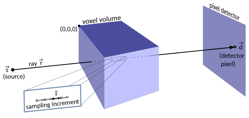
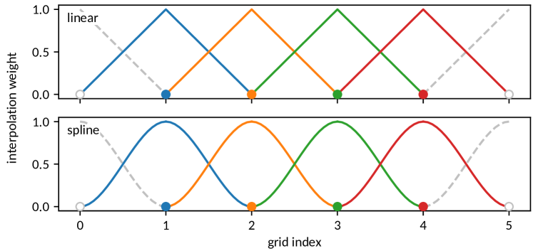
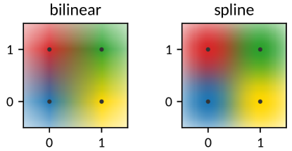
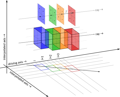
Figure 1: Ray casting through a volume along a line defined by two points $\vec{s}$ and $\vec{d}$ (upper left). On the right, driving-axis aligned sampling is illustrated on the grid scale. Integer steps along the driving axis imply increments of $\tilde{r}=\vec{r}/r_{m}$ along the actual path, with $\smash{1\leq\bigl{\|}\tilde{r}\bigr{\|}\leq\sqrt{3}}$. Due to the alignment with one designated axis, interpolation is required only within 4-voxel blocks extending along the remaining axes (four of such blocks are shown in different colors). Above, the corresponding sampling points $\vec{p}^{\,(i)}$ are illustrated within their sampling planes described by the respective nearest neighbour locations $\vec{v}^{(i,1-4)}$. On the center left, the one dimensional interpolation kernels resulting from Equations 13 and 14 are illustrated. Each marker represents a point on the grid, and the color-matched kernels represent the respective interpolation weights as a function of fractional position between grid points. The resulting two dimensional interpolation scheme is demonstrated below.

The basic sampling concept is illustrated in Figure 1. A ray emanating from a source at $\vec{s}$ traverses a voxel volume and hits a detector pixel at $\vec{d}$. Along its intersection with the volume, the latter will be sampled in steps of $\tilde{r}$, which will be concretized in the following. While the resulting scheme is equivalent to general driving axis based methods, the present vector representation allows for a unified treatment of all cases, such that the “driving axis”, which normally distinguishes different code branches, now only determines the orientation of sampling planes within a branchless sampling loop.

Given the positions of source $\vec{s}$ and detector pixel $\vec{d}$ relative to the volume origin, the integration path is characterized by the set of points $\vec{p}$

$$\vec{p} =\vec{s}+l\vec{r}$$ (1)

with

$$\vec{r} =\vec{d}-\vec{s}$$ (2)

and $l\in\mathbb{R}$ being the free parameter. The driving axis $m$ is then identified by the largest component of $\vec{r}$:

$$m=\underset{i}{\mathrm{argmax}}(|r_{i}|)\>.$$ (3)

The increment vector $\tilde{r}$ between successive sampling points will be chosen such that the resulting sampling points remain aligned with the driving axis, which holds for

$$\tilde{r}=\frac{\vec{r}}{r_{m}}\>.$$ (4)

Assuming that grid coordinates correspond here to non-negative memory indices, the first possible sampling point is defined by the intersection of the ray with a plane through the origin and perpendicular to the driving axis $m$, i.e.,

$$[\vec{s}+o\,\tilde{r}]_{m} \overset{!}{=}0$$ (5)

$$\Rightarrow o =-s_{m}$$

where $o$ is the distance between source and first sampling plane in units of the sampling increment $\bigl{\|}\tilde{r}\bigr{\|}$. $o$ will thus be termed “sampling offset”. The volume can now be sampled at points $\vec{p}^{\,(i)}$ along the defined path in unit steps of axis $m$ by evaluating

$$\vec{p}^{\,(i)}=(\vec{s}+o\,\tilde{r})+i\,\tilde{r}$$ (6)

for integer $i\in[0,i_{\max}$], where $i_{\max}$ is defined by the extent of the voxel grid along axis $m$. These sampling points can readily be used for linear interpolated sampling, as is e.g. directly provided by texture memory of modern GPUs.

III-B Interpolated sampling

When sampling from (GPU) main memory, the 4-neighborhood $\{\vec{v}^{(i,1)},\vec{v}^{(i,2)},\vec{v}^{(i,3)},\vec{v}^{(i,4)}\}$ of integer valued grid coordinates around each sampling point $\vec{p}^{\,(i)}$ needs to be explicitly enumerated. The driving axis component $p_{m}^{(i)}$ is, by construction of the sampling increment $\tilde{r}$ and offset $o$, guaranteed to be integer for all integer $i$. The remaining non-integer components necessarily lie between two integer ones along their respective coordinate axes. For each sampling point $\vec{p}^{\,(i)}$, the set of four neighboring voxels can thus be determined by regarding all combinations of floor and ceiling values of these non-integer components (with $\bigl{\lfloor}\,\bigr{\rfloor}$ and $\bigl{\lceil}\,\bigr{\rceil}$ being the floor and ceiling operators respectively):

$$\vec{v}^{(i,1)} =\bigl{\lfloor}p_{1}^{(i)}\bigr{\rfloor},\bigl{\lfloor}p_{2}^{(i)}\bigr{\rfloor},\bigl{\lfloor}p_{3}^{(i)}\bigr{\rfloor}$$ (7)

$$\vec{v}^{(i,2)} =\bigl{\lfloor}p_{1}^{(i)}\bigr{\rfloor},\bigl{\lceil}p_{2}^{(i)}\bigr{\rceil},\bigl{\lceil}p_{3}^{(i)}\bigr{\rceil}$$

$$\vec{v}^{(i,3)} =\bigl{\lceil}p_{1}^{(i)}\bigr{\rceil},\bigl{\lfloor}p_{2}^{(i)}\bigr{\rfloor},\bigl{\lceil}p_{3}^{(i)}\bigr{\rceil}$$

$$\vec{v}^{(i,4)} =\bigl{\lceil}p_{1}^{(i)}\bigr{\rceil},\bigl{\lceil}p_{2}^{(i)}\bigr{\rceil},\bigl{\lfloor}p_{3}^{(i)}\bigr{\rfloor}\>,$$

exploiting that

$$\bigl{\lfloor}p_{m}^{(i)}\bigr{\rfloor}=\bigl{\lceil}p_{m}^{(i)}\bigr{\rceil}=p_{m}^{(i)}\>.$$ (8)

Independent of $m\in\{1,2,3\}$, the vectors $\vec{v}^{(i,1-4)}$ define a group of four voxels in a plane perpendicular to the driving axis. Illustrations of the planes spanned by these nearest neighbor voxels around sampling points $\vec{p}^{\,(i)}$ are given in Figure 1. Special cases arise when either of the non-$m$ components of $\vec{p}^{\,(i)}$ happen to be also integer, which leads to redundant vectors among $\vec{v}^{(i,1-4)}$. Given the final objective of interpolation, these cases will be accounted for by adequate choice of the respective interpolation weights.

Interpolation will be based on scalar distance weights

$$w(d) ;\quad d\in[0,1]$$ (9)

$$\text{with}\quad w(1-d) =1-w(d)$$

with respect to the component wise distances of the contributing grid points next to a sampling point:

$$d_{k}^{(\mathrm{fl})} =p_{k}^{(i)}-\bigl{\lfloor}p_{k}^{(i)}\bigr{\rfloor}\,;\qquad d_{k}^{(\mathrm{cl})}=1-d_{k}^{(\mathrm{fl})}\>,$$ (10)

where the superscripts $(\mathrm{fl})$ and $(\mathrm{cl})$ indicate distances to the integer grid indices below and above the components $p_{k}^{(i)}$ of $\vec{p}^{\,(i)}$. The definition of $d_{k}^{(\mathrm{cl})}$ as complement to $d_{k}^{(\mathrm{fl})}$ guarantees correct interpolation weights also in the special case of integer components $p_{k}^{(i)}$, where floor and ceiling values coincide. When explicitly defining

$$w_{\mathrm{fl},k} =\mathrlap{w(d_{k}^{(\mathrm{fl})})}\hphantom{1-w_{\mathrm{fl},k}\quad}\text{for }k\neq m$$ (11)

$$w_{\mathrm{cl},k} =1-w_{\mathrm{fl},k}\quad\text{for }k\neq m$$

$$w_{\mathrm{fl},m} =w_{\mathrm{cl},m}=1$$

the interpolation weights $w^{(i,1-4)}$ for the respective voxels $\vec{v}^{(i,1-4)}$ can be conveniently represented as:

$$w^{(i,1)} =w_{\mathrm{fl},1}^{(i)}\cdot w_{\mathrm{fl},2}^{(i)}\cdot w_{\mathrm{fl},3}^{(i)}$$ (12)

$$w^{(i,2)} =w_{\mathrm{fl},1}^{(i)}\cdot w_{\mathrm{cl},2}^{(i)}\cdot w_{\mathrm{cl},3}^{(i)}$$

$$w^{(i,3)} =w_{\mathrm{cl},1}^{(i)}\cdot w_{\mathrm{fl},2}^{(i)}\cdot w_{\mathrm{cl},3}^{(i)}$$

$$w^{(i,4)} =w_{\mathrm{cl},1}^{(i)}\cdot w_{\mathrm{cl},2}^{(i)}\cdot w_{\mathrm{fl},3}^{(i)}$$

without requiring further explicit consideration of the particular driving axis $m$.

Two specific weighting functions shall be considered:

$$w_{\mathrm{lin}}(d) =1-d$$ (13)

$$w_{\mathrm{spl}}(d) =1-3d^{2}+2d^{3},$$ (14)

with $w_{\mathrm{lin}}$ reproducing classic multilinear interpolation and $w_{\mathrm{spl}}$ being a smooth spline function in the style of a smooth cosine window that ensures differentiability also at grid points, i.e., when $d=0$ or $d=1$. The practical consequences of the different interpolations schemes are later addressed in Sections IV-A–IV-B and Figures 2–3 therein.

Algorithm 1 combines the above considerations on volume traversal, implicit identification of sampling planes, and interpolation among the respective nearest neighbors into a single sampling loop. As can be verified by explicitly assuming different driving axes, the weighted sampling performed in lines 17–20 always correspond to a 2D-interpolation among the nearest neighbors of the respective sampling point within a plane perpendicular to the axis $m$.

1:$\mathbf{assuming:}$ $\vec{s},\vec{d}$ defined in units of voxel grid indices

2:$\vec{r}\leftarrow\vec{d}-\vec{s}$$\triangleright$ integration path orientation

3:$m\leftarrow\mathrm{argmax}_{i}(|r_{i}|)$$\triangleright$ $m$: major (driving) axis

4:$\tilde{r}\leftarrow\vec{r}/r_{m}$$\triangleright$ $\tilde{r}$: sampling increment vector

5:$o\leftarrow-s_{m}$ $\triangleright$ $o$: sampling offset, $\vec{s}$: ray source point

6:$i_{\max}\leftarrow$ volumeDimensions[$m$]$\triangleright$ number of sampling points

7:$a\leftarrow 0$$\triangleright$ $a$: accumulator variable

8:for $i=0\,..\,i_{\max}-1$ do$\triangleright$ iterate over sampling points

9:    $\vec{p}\leftarrow\vec{s}+(o+i)\cdot\tilde{r}$$\triangleright$ $\vec{p}$: current sampling point

10:    if $\vec{p}$ is in volume then

11:         $\mathrlap{\vec{p}_{\mathrm{fl}}}\hphantom{\vec{p}_{\mathrm{cl}}}\leftarrow\mathrm{floor}(\vec{p})$$\triangleright$ find lower voxel grid indices

12:         $\vec{p}_{\mathrm{cl}}\leftarrow\hphantom{\mathrm{floor}}\mathllap{\mathrm{ceil}}(\vec{p})$$\triangleright$ find upper voxel grid indices

13:         assert: $p_{\mathrm{fl},m}=p_{\mathrm{cl},m}=p_{m}$

14:         $\mathrlap{\vec{w}_{\mathrm{fl}}}\hphantom{\vec{w}_{\mathrm{cl}}}\leftarrow w(\vec{p}-\vec{p}_{\mathrm{fl}})$$\triangleright$ interpolation weights (Eqs. 13, 14)

15:         $\vec{w}_{\mathrm{cl}}\leftarrow\vec{1}-\vec{w}_{\mathrm{fl}}$ $\triangleright$ complementary weights

16:         w${}_{\mathrm{cl},m}\leftarrow w_{\mathrm{fl},m}\leftarrow 1$ $\triangleright$ special case: driving axis

17:         $a\leftarrow a+{}$volume$[\,\mathrlap{p_{\mathrm{fl},1}}\hphantom{p_{\mathrm{cl},1}}$, $\mathrlap{p_{\mathrm{fl},2}}\hphantom{p_{\mathrm{cl},2}}$, $\mathrlap{p_{\mathrm{fl},3}}\hphantom{p_{\mathrm{cl},3}}]$ $\cdot\left\|\tilde{r}\right\|\cdot w_{\mathrm{fl},1}\cdot w_{\mathrm{fl},2}\cdot w_{\mathrm{fl},3}$

18:         $a\leftarrow a+{}$volume$[\,\mathrlap{p_{\mathrm{fl},1}}\hphantom{p_{\mathrm{cl},1}}$, $p_{\mathrm{cl},2}$, $p_{\mathrm{cl},3}]$ $\cdot\left\|\tilde{r}\right\|\cdot w_{\mathrm{fl},1}\cdot w_{\mathrm{cl},2}\cdot w_{\mathrm{cl},3}$

19:         $a\leftarrow a+{}$volume$[\,p_{\mathrm{cl},1}$, $\mathrlap{p_{\mathrm{fl},2}}\hphantom{p_{\mathrm{cl},2}}$, $p_{\mathrm{cl},3}]$ $\cdot\left\|\tilde{r}\right\|\cdot w_{\mathrm{cl},1}\cdot w_{\mathrm{fl},2}\cdot w_{\mathrm{cl},3}$

20:         $a\leftarrow a+{}$volume$[\,p_{\mathrm{cl},1}$, $p_{\mathrm{cl},2}$, $\mathrlap{p_{\mathrm{fl},3}}\hphantom{p_{\mathrm{cl},3}}]$ $\cdot\left\|\tilde{r}\right\|\cdot w_{\mathrm{cl},1}\cdot w_{\mathrm{cl},2}\cdot w_{\mathrm{fl},3}$

21:    end if

22:end for.

Algorithm 1 Branchless ray casting through a cuboid voxel volume with axis aligned sampling and first order interpolation among four nearest neighbors. Scaling by $\bigl{\|}\tilde{r}\bigr{\|}$ accounts for the varying sampling distances depending on the orientation of the ray $\vec{r}$. 2D X-ray projection images of a volume are obtained by parallel evaluation for multiple rays defined by a focal point $\vec{s}$ and multiple detector pixel locations $\vec{d}$. Highest GPU cache efficiency is achieved when the driving axis $m$ does not coincide with the fastest changing index of the memory layout.

IV Results

IV-A Quality of projection images

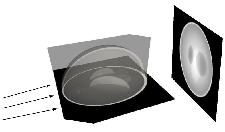
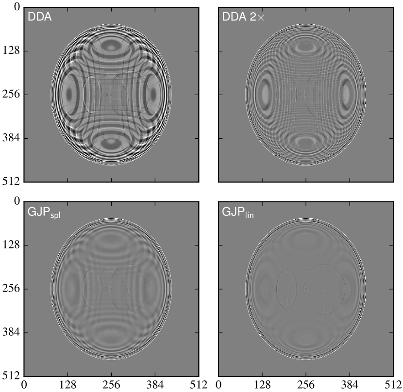
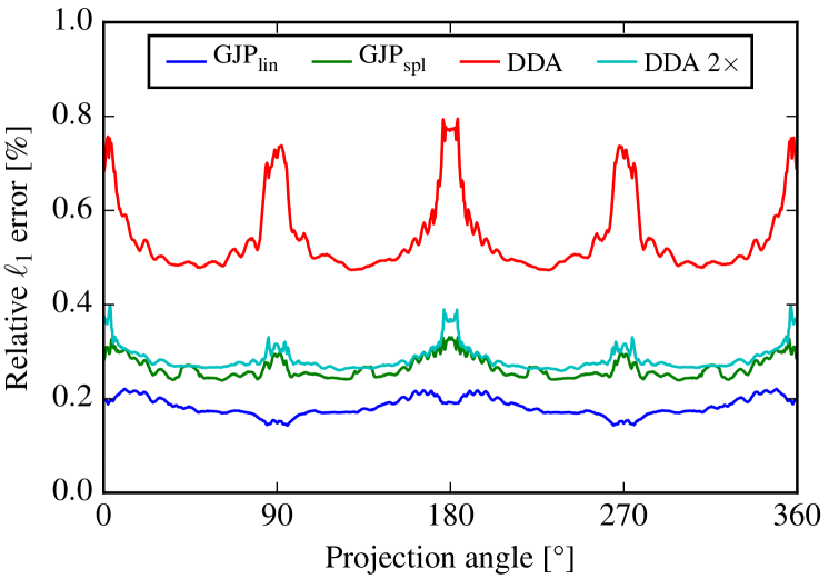
Figure 2: Approximation errors of different projection algorithms for a 10° conebeam geometry. Numeric projections of the rasterized Shepp Logan phantom (on a $512^{3}$ grid) onto a $512^{2}$ detector are compared to corresponding reference projections obtained by analytic integration of the ellipsoids defining the phantom. At the top, an illustration of the Shepp Logan phantom and the applied projection geometry is given. Below, example difference images for a frontal view are shown. On the bottom, the $\ell_{1}$ norm of these residuals, normalized to the $\ell_{1}$ norm of the analytic reference projection, is plotted for all projection angles of a circular scanning trajectory within the axial plane.

The performance with respect to adequate modeling of of ray-volume intersections is demonstrated on cone beam projections of a classic three dimensional Shepp Logan phantom based on the definition reproduced in [Schabel2006]. The phantom is described by a sum of ellipsoids, which can on the one hand be easily rasterized at any desired resolution and on the other hand allows the direct calculation of projection images by analytical evaluation of line integrals over the defining ellipsoids. A ground truth is thus available for comparison with respective numeric projections calculated from the rasterized version. In order to also adequately account for the extent and integrating nature of detector pixels, the reference projections are evaluated as an average over 64 line integrals between the focal spot and regular arrays of $8\times 8$ points within each detector pixel. Analogously, oversampling is applied also in the rasterization process of the phantom: It is rasterized on a regular grid of $512^{3}$ voxels, whereby each voxel value is determined as an average over $5\times 5\times 5$ regularly distributed samples of the function defining the phantom.

Following typical experimental conditions, a cone angle of 10° is modeled (i.e., the focal distance is about $5.7$ times the detector width), projecting the volume onto a square detector of $512^{2}$ pixels. In total, 803 ($\approx\frac{\pi}{2}512$) projection images from different orientations covering a full circle are computed, whereby the chosen number of projections corresponds to a common recommendation with regard to analytic tomographic reconstruction (cf. [Bugug2011]).

Figure 2 shows residual projection errors observed for various numeric projection approaches. Although the general occurrence of such residuals is generally expected due to the inherently approximative nature of discrete volume represenations, the adequacy of a projection model may reasonably be measured by its ability to keep such residuals minimal. Siddon’s pencil beam projection model, realized using the DDA algorithm, exhibits most artifacts, particularly in cases where rays run roughly parallel to grid axes. In these situations the model of pencil beams intersecting box-shaped voxels is equivalent to nearest neighbor sampling. When oversampling the DDA by a factor of two in each dimension in order to approximate a finite beam extent, i.e. tracing and averaging over four rays per detector pixel, the resulting projection residuals become comparable to those of the non-oversampled GJP_spl algorithm using spline interpolation, although the latter further shows a considerable reduction of high frequency artifacts. The best results are, despite the kinked interpolation kernel, achieved by the liner interpolating GJP_lin algorithm.

IV-B Quality of iterative tomographic reconstructions

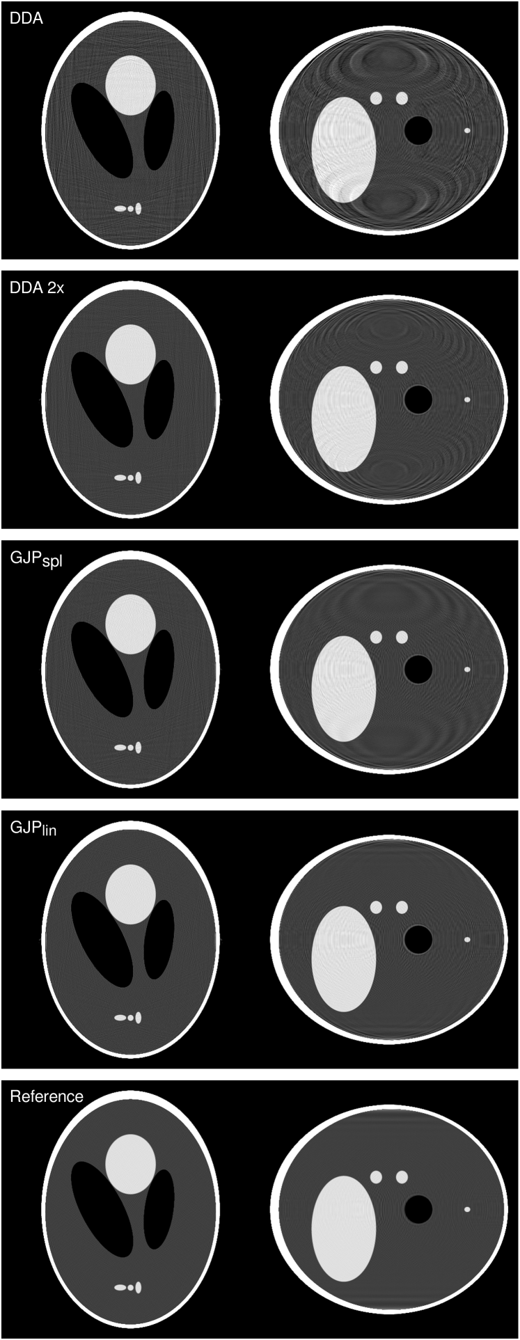
Figure 3: Axial (left) and sagittal (right) central slices of iterative SART reconstructions (10 iterations) on a discrete voxel grid from analytic projections of a 3D Shepp Logan phantom using different numeric projection methods within the iterative process. The chosen grayscale window shows a range of [0.16,0.32] out of the maximal range of [0,1]. Limitations of the discrete forward models (cf. Fig. 2) manifest themselves in the final reconstruction result. At the bottom, a reconstruction from perfect input data (synthesized with GJP_lin from the rasterized Shepp Logan phantom) is shown for reference, demonstrating the artifacts expected from the reconstruction process itself. Wavy features at the sagittal top and bottom represent cone beam artifacts.

As iterative reconstruction techniques such as SART ([AndersenKak1984], “Simultaneous Algebraic Reconstruction Technique”) subsequently enforce consistency of the reconstructed volume with each experimentally observed projection image based on a given forward model (formally represented by a matrix $\boldsymbol{A}$, applied to a vector of volume elements $\boldsymbol{f}$, yielding a set of line integrals $\boldsymbol{g}$), inaccuracies of the respective discrete forward projectors will directly translate to artifacts in the reconstruction result. In contrast to typical artifacts arising when reconstructing from an under-determined system of equations, e.g., when reconstructing from too few projections, deficiencies of the projection model defining the system matrix $\boldsymbol{A}$ inherently do not lie in its null space, and can therefore not, without loss of resolution, be compensated by typical regularization approaches that are otherwise used to suppress artifacts emerging in the null space of $\boldsymbol{A}$, i.e., in image domains that are not affected by $\boldsymbol{A}$ and its defining projection model.

In order to illustrate the practical consequences, multiple SART reconstructions are compared using different projection algorithms. In general, such experiments typically suffer either from unrelated artifacts when working with actual experimental data, or from the “inverse crime” that is often committed when synthesizing experimental data based on the same algorithms that are also used in the subsequent reconstruction procedure. Both issues can however be avoided in the case of the Shepp-Logan phantom due to the possibility to analytically calculate its projections without prior rasterization, as has been done already for the previous benchmark.

Figure 3 shows central axial and sagittal slices of respective SART reconstructions on a $512^{3}$ voxel grid of the Shepp-Logan phantom from analytically calculated projections as described previously. As volume rasterization is here only introduced with the discrete imaging model fundamental to iterative reconstruction techniques, the observed reconstruction artifacts can be largely attributed to the employed discrete projection method. While other parameters such as iteration count or the interpolation scheme of the voxel based backprojector can also be argued to affect the reconstruction outcome, it should nevertheless be without doubt that these, in contrast to the forward model, do not actually explicitly define the properties of the solution. The bottom panel of Fig. 3 illustrates the isolated effect of the present reconstruction procedure by using ideal input data synthesized with the same forward model (GJP_lin) also used for iterative reconstruction. In contrast to artifacts arising from the forward model itself, pure reconstruction artifacts can generally be suppressed by regularization techniques, which have here explicitly not been applied to avoid ambiguities in the interpretation of the presented results.

In accordance with the previously found projection errors shown in Fig. 2, the reconstruction quality is found to be worst for the non-oversampling DDA, comparable for 2-fold oversampled DDA and GJP_spl and best for GJP_lin. Although it is out of the scope of the present work to explicitly demonstrate the effect of each SART parameter, the reader shall however be assured that variations in iteration count, relaxation factor and backprojection interpolation scheme have been confirmed to not fundamentally change the relative performance of different forward models. This is in accordance with the preceding reasoning attributing the differing artifact patterns to differing discretization errors among the various methods.

Finally, these results are further independent of additive noise, which has here intentionally not been regarded. As SART is, despite being iterative, a linear reconstruction technique, additive terms to the projection images can generally be considered independently and will, although adding to the reconstruction result, not fundamentally alter it.

IV-C Projection speed

Run time performance is evaluated for projections of a cylindric volume (as common for tomographic reconstructions) within a cubic bounding box of $512^{3}$ voxels onto a $512^{2}$ pixel detector. The sampling offset $o$ marking the first sampling point and the total number of sampling points $i_{\max}$ are adapted to ray-cylinder intersections as opposed to ray-boundingbox intersections to this purpose. The performance of Algorithm 1 is benchmarked against the branchless DDA formulation given by [Xiao2012]. The volume is stored in 32bit floating point format in either main- or texture memory of the graphics processing unit. For the case of texture memory, also hardware provided interpolation is tested. As typical for computed tomography setups, projections are performed for a multitude of source and detector orientations over the full angular range of $360\text{\textdegree}$ on a circular trajectory around the volume center. The rotational axis is aligned parallel to the fastest index of the memory layout (i.e., the last dimension in the case of Fortran-style memory order, or the first dimension in the case of C-style memory order). For each individual configuration of source and detector, the run time is optimized over a wide range of possible thread block or work group size parameters (CUDA and OpenCL terminology respectively). This eliminates the potential influence of technicalities introduced by the parallelization schemes of graphics processors. Measured execution times further exhibit a variance of up to 10% when running the same code multiple times due to dynamic performance adaptions related to temperature management. Reported are the fastest measured times for each algorithm.

	DDA			DDA 2$\times$			GJPlin			GJPhwlin
	GTX970	GTX1080		GTX970	GTX1080		GTX970	GTX1080		GTX970	GTX1080
Tex.	4.59 ms	3.46 ms		15.2 ms	6.74 ms		4.97 ms	2.40 ms		3.28 ms	2.23 ms
	118 GB/s	157 GB/s		143 GB/s	323 GB/s		334 GB/s	686 GB/s		502 GB/s	740 GB/s
RAM	4.39 ms	5.20 ms		15.7 ms	7.65 ms		5.69 ms	2.70 ms		—	—
	123 GB/s	104 GB/s		139 GB/s	285 GB/s		292 GB/s	609 GB/s		—	—

Table I: Average projection speed in milliseconds and memory access rates in gigabytes per second for 2D projections of a cylindrical volume within a $512^{3}$ bounding box onto a $512^{2}$ detector in a 10° conebeam setup measured an Nvidia GTX 970 and GTX 1080 GPU.

Table I lists the so evaluated run times as averages over 360 equidistant projection angles for two GPU models. As a measure for GPU occupancy it further lists average memory access rates based on the total runtime and the amount of accessed voxels by each raytracing algorithm respectively. Although the latter is not strictly known in the case of GJP_hwlin due to unknown implementation details within the GPU, it is reasonably assumed to be the same as for GJP_lin.

A number of interesting conclusions can be drawn from the observed timings: First of all, the DDA algorithm can only benefit from newer hardware (GTX 1080) in the oversampled case. Oversampling increases the number of duplicate accesses to the same voxels by parallel threads handling neighboring rays, wherefore it can be reasonably assumed that the oversampled DDA better profits from memory caches. The additional computational overhead associated with oversampling appears to be a limiting factor on older hardware in contrast, where the overall runtime increases almost linear with the amount of traced rays. This assessment is consistent with the observation that the DDA algorithm does not profit from optimized accesses to read only texture memory. The GJP algorithm in contrast is able to outperform even the regular DDA algorithm by a factor of up to 2, despite accessing about twice as much memory on average. The driving axis aligned sampling scheme of the GJP ensures that neighboring threads partially access the same voxels in the course of interpolated sampling, thereby exploiting memory caches even better than the oversampled DDA. The additional speedup observed when simplifying the GJP algorithm even further (by using the intrinsic interpolation capabilities of texture memory) indicates that it operates close to the limits both of the computational resources and the available memory bandwidth.

V Discussion and Conclusion

The calculation of projections from discrete volumes is a core aspect of iterative reconstruction techniques, both with respect to reconstruction speed and quality. Although a remarkable variety of approaches to the advanced modeling of ray-volume intersections has been presented in previous literature, the demand for maximal parallelizability and computational efficiency on modern graphics processors immediately collapses the wide palette of choices to ray driven methods with strongly confined sampling kernels. “Ray driven” thereby implies a sampling loop iteratively traversing the voxel grid along defined paths (rays) between focal point and detector pixels, and “strongly confined” implies the evaluation of only the immediate neighborhood around each sampling point. For the traversal of regular grids, two methods can be named: the digital differential analyzer (DDA) algorithm [AmanatidesWoo1987], traversing the grid in unevenly spaced steps from intersection to intersection with any of the orthogonal grid planes, and methods traversing the grid in equidistant steps aligned with a designated driving axis. The former technique allows to precisely determine line-box intersection lengths and corresponds to the much cited pencil-beam X-ray imaging model given by Siddon [Siddon1985], while the latter technique is typically combined with interpolated sampling and then corresponds to the competing model proposed in the context of tomographic reconstruction by Joseph [Joseph1982].

A branchless formulation of a Joseph type interpolating volume projection algorithm has been derived here, with the particular benefit of being extremely simple, which is a general prerequisite for maximal computational efficiency. Driving axis aligned sampling ensures an optimal amount of sampling points along each path in the sense that voxels are neither skipped nor oversampled. The resulting synchronous progression of parallel rays through the voxel grid thereby ensures high cache hit rates without explicitly constraining the exact imaging geometry (as opposed to e.g. the cache optimized Siddon’s algorithm proposed by [ThompsonLionheart2014], or the symmetry exploiting projection model given by [Scheins2015]). Interpolated sampling among the remaining dimensions has been argued, besides being a practical necessity, to be consistent with ideas on exact modeling of X-ray projections based on normalized radial basis functions or projection footprints. Approximate matching of the voxel grid spacing to the average density of rays between focal point and detector array thereby ensures an adequate modeling of beam width, implicitly reproducing the integrating nature of detector pixels of finite extent without requiring far ranging interpolation kernels or oversampled ray casting. In accordance with assessments given in previous literature, higher order effects such as cone beam related variations in beam extent can be safely neglected in the modeling. (cf.  e.g. [Nuyts2013, HofmannKachelriess2014])

The performed benchmarks compared a number of self-suggesting variants of both ray casting algorithms with respect to artifacts and computational efficiency, addressing the recurring questions of adequate beam shape modeling and the role of the chosen interpolation kernel. The results indicate that no tradeoff needs to be made between computational efficiency and fitness for the purpose: the proposed simple and efficient branchless 3D Joseph projector employing linear interpolation is found to clearly perform best both with regard to approximation of the ground truth and with regard to efficiency, operating in the range of the theoretic maximum capabilities of the employed hardware.

A recurring concern with regard to local interpolation exists in situations where a sufficient matching of the voxel grid resolution to the detector resolution is seemingly impossible. Such situations can e.g. arise when attempting to combine isotropic volume sampling with highly asymmetric detector pixels. It is in such cases obviously generally possible to cast an adequate amount of rays per detector bin ensuring sufficient coverage of the voxel grid, i.e., to adequately oversample the detector image. Similarly, the voxel shape may be chosen non-square (in terms of spatial units) to adequately match the detector properties, which in units of grid indices does not alter the discussed algorithms. Arguments questioning the representativeness of the Shepp-Logan phantom, that has here been chosen for the sake of analytic integrability, may be countered by noting that the observed artifacts arise at extended material boundaries of moderate curvature, i.e., a situation that is typical to CT applications.

The proposed formulation of a linearly interpolating Joseph-type projection algorithm may eventually be considered a favorable choice in many regards (simplicity of implementation, computational efficiency, and fitness for the purpose) for typical CT reconstruction applications, in particular as compared to the competing DDA algorithm, and further considering that oversampling (i.e., increasing the density of traced rays) generally remains an option.