Diffusive escape through a narrow opening: new insights into a classic problem

Abstract

We study the mean first exit time $T_{\varepsilon}$ of a particle diffusing in a circular or a spherical micro-domain with an impenetrable confining boundary containing a small escape window (EW) of an angular size $\varepsilon$. Focusing on the effects of an energy/entropy barrier at the EW, and of the long-range interactions (LRI) with the boundary on the diffusive search for the EW, we develop a self-consistent approximation to derive for $T_{\varepsilon}$ a general expression, akin to the celebrated Collins-Kimball relation in chemical kinetics and accounting for both rate-controlling factors in an explicit way. Our analysis reveals that the barrier-induced contribution to $T_{\varepsilon}$ is the dominant one in the limit $\varepsilon\to 0$, implying that the narrow escape problem is not “diffusion-limited” but rather “barrier-limited”. We present the small-$\varepsilon$ expansion for $T_{\varepsilon}$, in which the coefficients in front of the leading terms are expressed via some integrals and derivatives of the LRI potential. On example of a triangular-well potential, we show that $T_{\varepsilon}$ is non-monotonic with respect to the extent of the attractive LRI, being minimal for the ones having an intermediate extent, neither too concentrated on the boundary nor penetrating too deeply into the bulk. Our analytical predictions are in a good agreement with the numerical simulations.

I Introduction

The narrow escape problem (NEP) is ubiquitous in molecular and cellular biology and concerns diverse situations when a particle, diffusing within a bounded micro-domain, has to search for a small specific target on the domain’s boundary lin ; zhou ; grig ; yan2 ; schuss2 ; ben1 ; kol1 ; kol2 . A particle can be an ion, a chemically active molecule, a protein, a receptor, a ligand, etc. A confining domain can be a cell, a microvesicle, a compartment, an endosome, a caviola, etc, while the target can be a binding or an active site, a catalytic germ, or a narrow exit to an outer space, from which case the name of the problem originates. The outer space can be an extracellular environment or, as considered in recent analysis of diffusion and retention of $Ca^{2+}$-calmoduline-dependent protein kinase II in dendritic spines byr ; dag , be the dendrite itself while the narrow tunnel is a neck separating the spine and the dendrite. For all these stray examples, called in a unified way as the NEP, one is generally interested to estimate the time needed for a particle, starting from a prescribed or a random location within the micro-domain, to arrive for the first time to the location of the target. The history, results, and important advances in understanding of the NEP have been recently reviewed schuss ; new ; holc ; holc2 ; holc3 .

Early works on NEP were focused on situations when the confining boundary is a hard wall, i.e., is perfectly reflecting everywhere, except for the escape window (or other specific target), which is also perfect in the sense that there is neither an energy nor even an entropy barrier which the particle has to overpass in order to exit the domain (or to bind to the specific site). In this perfect, idealised situation, the mean first exit time (MFET) through this window is actually the mean first passage time (MFPT) to its location. This MFPT was calculated by solving the diffusion equation with mixed Dirichlet-Neumann boundary conditions ward .

Capitalising on the idea that the particle diffusion along the bounding surface can speed up the search process, set forward for chemoreception by Adam and Delbrück adam and for protein binding to specific sites on a DNA by Berg et al. berg , as well as on the idea of the so-called intermittent search ben2 ; ben3 ; osh1 ; osh2 ; osh3 ; met2 ; met ; alj , more recent analysis of the NEP dealt with intermittent, surface-mediated diffusive search for an escape window, which also was considered as perfect, i.e. having no barrier at its location. The MFPTs were determined, using a mean-field osh20 and more elaborated approaches greb1 ; greb2 ; greb3 ; greb4 ; budde0 ; albe ; budde ; ben4 ; ber1 ; ber2 , as a function of the adsorption/desorption rates, and of the surface ($D_{\rm surf}$) and the bulk ($D$) diffusion coefficients. It was found that, under certain conditions involving the ratio between $D$ and $D_{\rm surf}$, the MFPT can be a non-monotonic function of the desorption rate, and can be minimised by an appropriate tuning of this parameter greb1 ; greb2 ; greb3 ; greb4 ; budde0 ; albe ; budde ; ben4 ; ber1 ; ber2 .

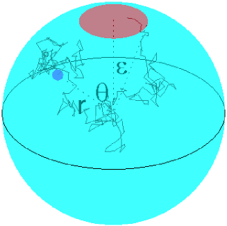
Figure 1: Schematic picture of the narrow escape problem : An escape window (EW) is a cap of polar angle $\varepsilon$ and diameter $a=2R\sin\varepsilon$ located at the North pole of a sphere of radius $R$. A diffusive particle starts from a point $(r,\theta)$ (small filled circle) and eventually arrives to the EW.

In this paper we analyse the problem of a narrow escape of a Brownian particle through a small window located on the boundary of a three-dimensional spherical or a two-dimensional circular domain (see Fig. 1) taking into account explicitly a finite energy and/or an entropy barrier at the EW and the presence of long-range (beyond the usual hard-core repulsion) particle-boundary interactions characterised by a radially-symmetric potential $W(r)$. We will use the term “escape window” (EW) in what follows, but clearly our results will also apply to situations when this targeted area is an extended binding region or an active site. Our motivations here are as follows:

i) The adsorption/desorption rates cannot be tuned independently as they are linked on the microscopic level by the particle-boundary interactions. As a consequence, not all values of the latter parameters are physically possible and it is unclear a priori if the non-monotonic behaviour of the MFPT observed in earlier works can indeed take place in physical systems.

ii) If diffusion along the surface may indeed speed up the search for the EW in case of contact attractive interactions with the surface, it is natural to expect that, in the presence of long-range attractive interactions with the surface, these typical search times will be further reduced since the particle will feel the surface on longer distances and will experience a drift towards it. Moreover, on intuitive grounds, one may expect the existence of some optimal extent of the interaction potential since for potentials with an infinite extent, the problem will reduce to the one with purely hard-wall interactions. Consequently, it may turn out that the mean search time will be a non-monotonic function of the extent of the interaction potential.

iii) In realistic systems not every passage to the EW results in the escape from the domain, but this event happens only with some finite probability, due to an energy or an entropy barrier, the latter being dominated by the window size zhou ; paolo1 ; paolo2 . Similarly, chemical reactions with a specific site on the boundary of the micro-domain are also never perfect but happen with a finite probability defining some rate constant $\kappa$ col . This rate constant has already been incorporated into the theoretical analysis of the NEP for systems with hard-wall or contact interactions with the surface budde , but to the best of our knowledge, its effect on the MFET has never been appreciated in full detail. We will revisit this analysis for the situations with (and without) the long-range particle-boundary interaction.

These are the focal questions of our analysis. We proceed to show that the MFET naturally decomposes into two terms: the mean first passage time to the EW and the time necessary to overcome the barrier at the entrance to the EW. We realise that the MFPT to the EW is indeed an optimisable function of the interaction potential, when these interactions are attractive, the effects being more pronounced for spherical micro-domains than for circular micro-domains. More specifically, we find that while the MFPT appears to be a monotonic function of the strength of the interaction potential at the boundary, it exhibits a minimum with respect to the spatial extent of the potential, which defines the force acting on the particle in the vicinity of the boundary. We show that the optimum indeed occurs for interactions of an intermediate extent, such that they are neither localised too close to the confining boundary, nor extend too deeply into the bulk of the micro-domain. In a way, the observation that the MFPT exhibits a non-monotonic behaviour as the function of the extent of the potential is consistent with the earlier predictions for the optimum of the MFPT with respect to the desorption rate, based on the models with intermittent motion. As a matter of fact, the extent of the potential defines the barrier against desorption from the confining boundary and hence, controls the desorption rate. There are, however, some discrepancies between our predictions here and those based on intermittent modelling on which we will comment in what follows.

Further on, focusing on the effect of a barrier at the entrance to the EW, which is always present in realistic situations, we demonstrate that the contribution to the MFET stemming out from the passage through the barrier is more singular in the limit $\varepsilon\to 0$ than the MFPT to the EW. This means that, mathematically speaking, the former provides the dominant contribution to the MFET implying that the narrow escape problem is not “diffusion-limited” but rather “barrier-limited”. This observation has significant consequences for chemical and biological applications.

Our analytical approach is based on the backward Fokker-Planck equation with a long-range potential that governs the MFET to an imperfect (partially-reflecting, $\kappa<\infty$) EW for a particle starting from a given location within the micro-domain. We obtain an explicit approximate solution of the resulting mixed boundary value problem by resorting to an approximation devised originally by Shoup, Lipari and Szabo shoup for the analysis of reaction rates between particles with inhomogeneous reactivity solc . Within this approximation, the exact boundary conditions are replaced by some effective ones, reducing the problem to finding self-consistent solutions. The original self-consistent approximation was shown to be in a good agreement with numerical solutions of the original problem shoup ; trey .

We adapt this approximation to the NEP and also incorporate the long-range potential interactions between the particle and the boundary of the confining domain. Our theoretical predictions, based on this self-consistent approximation, will be checked against available exact asymptotic results for the case when the boundary is an impenetrable hard wall (long-range interactions are absent) and when there is no barrier at the entrance to the EW. For the general case, we will verify our analytical predictions by extensive Monte Carlo simulations and an accurate numerical solution of the original mixed boundary problem by a finite elements method.

The paper is organised as follows: In Sec. II we describe our model and introduce the main idea of the self-consistent approximation (SCA). In Sec. III we obtain the solution of the NEP with the modified boundary conditions, as prescribed by the SCA. In Sec. IV we first present the general expressions for the MFET for three-dimensional spherical and two-dimensional circular micro-domains, for arbitrary particle-wall interactions, an arbitrary $\kappa$ and the EW of an arbitrary angular size. Discussing its physical significance, we highlight the crucial role of the partial reactivity and its effect on the MFET. Further on, we show that in the narrow escape limit $\varepsilon\to 0$ one can straightforwardly derive an asymptotic small-$\varepsilon$ expansion for the MFET in which the expansion coefficients of the leading terms are explicitly defined via some integrals and derivatives of a rather arbitrary interaction potential. Lastly, on example of a representative triangular-well potential, we discuss the role of repulsive and attractive particle-boundary interactions and also demonstrate that the contribution to the MFET due to the diffusive search for the location of the EW (i.e., the MFPT to the EW), can be optimised by an appropriate tuning of the spatial extent of the interaction potential. We also analyse here some subtle issues related to the applicability of the Adam-Delbrück dimensionality reduction scheme adam . Section V concludes the paper with a brief recapitulation of our most significant results. Mathematical and technical details are presented in Supplemental Materials (SM), where we describe the numerical approaches used to verify our analytical predictions (SM1); derive the asymptotic small-$\varepsilon$ expansions and determine the asymptotic behaviour for short-range potentials (SM2); present solutions in absence of particle-wall interactions (SM3); and discuss the particular case of a triangular-well interaction potential for three-dimensional (SM4) and two-dimensional (SM5) micro-domains.

II Model and basic equations

Consider a point particle diffusing, with a diffusion coefficient $D$, in a three-dimensional sphere (3D case) of radius $R$ or a two-dimensional disk (2D case) of radius $R$, containing on the confining boundary a small EW characterised by a polar angle $\varepsilon$ and having a diameter $a=2R\sin\varepsilon$, see Fig. 1. We stipulate that, in addition to the hard-core repulsion at the boundary, the particle interacts with the confining wall via a radially-symmetric potential $W(r)$. We hasten to remark that an assumption that the interaction potential $W(r)$ depends only on the radial distance from the origin is only plausible in the narrow escape limit, i.e., when the polar angle is small ($\varepsilon\ll\pi$) or, equivalently, the linear extent $a$ of the EW is much smaller than the radius $R$. Otherwise, the interaction potential can acquire a dependence on the angular coordinates. Therefore, from a physical point view, this model taking into account the long-range interactions with the boundary in a spherically-symmetric form is representative only when $\varepsilon\ll\pi$. On the other hand, for situations with $W(r)\equiv 0$ the latter constraint can be relaxed and our analysis is applicable for any value of $\varepsilon$.

We are mainly interested in the MFET through the EW, $T_{\varepsilon}$, from a uniformly distributed random location, sometimes called the global MFET bonito and defined as

$$T_{\varepsilon}=\dfrac{1}{V_{d}}\int_{\Omega}dV_{d}\,t(r,\theta)\,,$$ (1)

where $V_{d}$ is the volume of the micro-domain $\Omega$ ($V_{3}=4\pi R^{3}/3$ in 3D case and $V_{2}=\pi R^{2}$ for 2D case) and $t(r,\theta)$ is the mean time necessary for a particle, started from some fixed location $(r,\theta)$ inside the domain, to exit through the EW. Due to the symmetry of the problem, $t(r,\theta)$ depends on the radial distance $r$ to the origin ($0\leq r\leq R$) and polar angle $\theta$ ($0\leq\theta\leq\pi$) but is independent of the azimuthal angle $\phi$ for the 3D case. In the 2D case, the reflection symmetry of the circular micro-domain with respect to the horizontal axis allows one to restrict the polar angle to $(0,\pi)$ as well. Although we focus in this paper exclusively on the global MFET $T_{\varepsilon}$, the SCA yields the explicit form of $t(r,\theta)$ too.

The function $t=t(r,\theta)$ satisfies the backward Fokker-Planck equation. For the 3D case, the MFET $t$ obeys

$$t^{\prime\prime}+\left(\frac{2}{r}-U^{\prime}\right)t^{\prime}+\frac{1}{r^{2}\sin\theta}\frac{\partial}{\partial\theta}\left(\sin\theta\frac{\partial t}{\partial\theta}\right)=-\frac{1}{D}\,,$$ (2)

where the prime here and henceforth denotes the derivative with respect to the variable $r$, and $U(r)$ is a dimensionless, reduced potential: $U(r)=\beta W(r)$, where $\beta$ is the reciprocal temperature measured in the units of the Boltzmann constant. For the 2D case, the MFET $t$ is governed by

$$t^{\prime\prime}+\left(\frac{1}{r}-U^{\prime}(r)\right)t^{\prime}+\frac{1}{r^{2}}\frac{\partial^{2}t}{\partial\theta^{2}}=-\frac{1}{D}.$$ (3)

In both cases, the backward Fokker-Planck equation is to be solved subject to the reflecting boundary condition which holds everywhere on the wall ($r=R$), except for the location of the EW, on which a partially-adsorbing boundary condition is imposed. For the backward Fokker-Planck equation, these mixed boundary conditions have the form:

$$-\left.D\,t^{\prime}\right|_{r=R}=\begin{cases}\kappa\,t(R,\theta),\qquad 0\leq\theta\leq\varepsilon,\cr 0,\hskip 51.21495pt\varepsilon<\theta\leq\pi,\end{cases}$$ (4)

where $\kappa$ is the above mentioned proportionality factor (in units length/time), which accounts for an energy or an entropy barrier at the entrance to the EW. If such a barrier is absent, $\kappa=\infty$ and one has a perfectly adsorbing boundary condition at the location of the EW, in which case the first line of (4) becomes $t(R,\theta)=0$ for $0\leq\theta\leq\varepsilon$. Evidently, in this case $T_{\varepsilon}$ is entirely determined by the first passage to the EW.

Within the context of chemical reactions with an active site located on the inner surface of the micro-domain, the condition in the first line of (4) can be considered as the partially-reflecting reactive boundary condition put forward in the seminal paper by Collins and Kimball col , and then extensively studied in the context of chemical reactions Sano79 ; Sapoval94 ; Grebenkov06 ; Singer08 ; Bressloff08 and search processes Grebenkov10a ; Grebenkov10b ; budde . In this framework, $\kappa$ can be written down as $\kappa=K/(4\pi R^{2}s_{g})$, where $K$ is the usual elementary reaction act constant (in units of volume times the number of acts per unit of time within this volume) and $s_{g}=\sin^{2}(\varepsilon)$ is the geometric steric factor characterising the fraction of the boundary area “covered” by the active site, so that $4\pi R^{2}s_{g}$ is simply the area of the active site. In turn, $K$ can be writtenberd as $K=\textit{f}\,V_{s}$ (see also the discussion in pop ), where f is the rate describing the number of reaction acts per unit of time within the volume $V_{s}$ of the reaction zone around an active site. If the reaction takes place within a segment of a spherical shell, defined by $R-\rho\leq r\leq R$ and $\theta\in(0,\varepsilon)$, where $\rho$ is the capture radius, one has $V_{s}=4\pi R^{2}\rho s_{g}$, so that $\kappa=\textit{f}\,\rho$. Clearly, a similar argument holds for the case of the EW with an energy barrier; in this case f can be interpreted as the rate of successful passages through the EW and is dependent on the energy barrier via the standard Arrhenius equation.

Last but not least, even when the confining boundary is a structureless hard wall so that an energy barrier is absent, a particle, penetrating from a bigger volume (micro-domain) to a narrower region of space, will encounter an entropy barrier $\Delta S$ at the entrance to the EW; in this case $\beta\Delta S\sim\ln(a/R)$ paolo1 ; paolo2 , $a$ being the lateral size of the escape window. This suggests, in turn, that $\kappa$, associated with an entropy barrier, depends linearly on $a$ and hence, linearly on $\varepsilon$. Therefore, for realistic situations one may expect that $\kappa$ associated with an entropy barrier is rather small, and gets progressively smaller when $\varepsilon\to 0$, becoming a rate-controlling factor. However, the absolute majority of earlier works on the NEP has been devoted so far to the limit $\kappa=\infty$, which corresponds to an idealised situation when there is neither energy, nor even entropy barrier at the entrance to the EW so that the particle escapes from the micro-domain upon the first arrival to the location of the EW. In this case the MFET is just the MFPT to the EW. As we will show, even if $\kappa$ is independent of $\varepsilon$, the passage through the barrier provides the dominant contribution to the MFET in the narrow escape limit $\varepsilon\to 0$.

Our approach to the solution of the mixed boundary-value problem in (2, 4) for the 3D case or in (3, 4) for the 2D case in the presence of a general form of the reduced potential $U(r)$ hinges on the SCA developed by Shoup, Lipari and Szabo shoup , who studied rates of an association of particles (e.g., ligands), diffusing in the bath outside of an impenetrable sphere without LRI potential (i.e., $U(r)\equiv 0$), to some immobile specific site covering only a portion of the outer surface of this sphere. Within this approximation one replaces the actual, mixed, partially adsorbing boundary condition in the first line of (4) by an effective one – a condition of a constant flux through the boundary at the location of the EW. More specifically, the mixed boundary condition in (4) is replaced by an inhomogeneous Neumann boundary condition:

$$\left.Dt^{\prime}\right|_{r=R}=Q\,\Theta(\varepsilon-\theta)\,,$$ (5)

where $\Theta(\theta)$ is the Heaviside function and $Q$ is the unknown flux which is to be determined self-consistently using an appropriate closure relation.

It is important to emphasise two following points: (i) the solution of the modified problem (2, 5) is defined up to a constant while the solution of the original problem (2, 4) is unique. However, in the narrow escape limit $\varepsilon\to 0$, the leading terms of the MFET diverge so that a missing constant would give a marginal contribution. (ii) the replacement of the boundary condition (4) by an effective one (5) does not guaranty, in principle, that the solution $t$ will be positive in the vicinity of the EW, since the effective boundary condition requires that (4) holds only on average (see also SM3). We will show that this approximation provides nonetheless accurate results for the global MFET with zero and non-zero $U(r)$.

III Self-consistent approximation

In this section we adapt the SCA for the NEP and also incorporate within this approach the long-range potential interactions with the confining boundary . Within this extended approach, we derive general expressions for $T_{\varepsilon}$ for arbitrary potentials in both 2D and 3D cases, as functions of the radius $R$ of the micro-domain, the angular size $\varepsilon$ of the EW, the constant $\kappa$, and the bulk diffusion coefficient $D$.

III.1 3D Case

The general solution of (2) can be written as the following expansion

$$t(r,\theta)=t_{0}(r)+\sum\limits_{n=0}^{\infty}a_{n}g_{n}(r)P_{n}(\cos(\theta))\,,$$ (6)

where $P_{n}(\cos(\theta))$ are the Legendre polynomials, $a_{n}$ are the expansion coefficients which will be chosen afterwards to fulfil the boundary conditions, $g_{n}(r)$ are the radial functions obeying

$$g^{\prime\prime}_{n}(r)+\left(\frac{2}{r}-U^{\prime}(r)\right)g^{\prime}_{n}(r)-\frac{n(n+1)}{r^{2}}g_{n}(r)=0\,,$$ (7)

and lastly, $t_{0}(r)$ is the solution of the inhomogeneous problem that can be written down explicitly as

$$t_{0}(r)=\frac{1}{D}\int\limits_{r}^{c_{1}}dx~{}\frac{e^{U(x)}}{x^{2}}\int\limits_{c_{2}}^{x}dy~{}y^{2}e^{-U(y)},$$ (8)

where $c_{1}$ and $c_{2}$ are two adjustable constants. We set $c_{2}=0$ to ensure the regularity of solution at $r=0$. In order to fix the constant $c_{1}$, we impose the Dirichlet boundary condition at $r=R$ to get

$$t_{0}(r)=\frac{1}{D}\int\limits_{r}^{R}dx~{}\frac{e^{U(x)}}{x^{2}}\int\limits_{0}^{x}dy~{}y^{2}e^{-U(y)}.$$ (9)

We emphasise that the Dirichlet boundary condition for $t_{0}(r)$ is chosen here for convenience only. As mentioned earlier, the solution of the modified problem (2, 5) is defined up to a constant which can be related to the constant $c_{1}$ here. An evident advantage of such a choice is that $t_{0}(r)$ in (9) is the exact solution of the original problem in case when $\varepsilon=\pi$ (i.e., the EW is the entire boundary of the sphere).

We turn next to the radial functions $g_{n}(r)$ defined in (7). For $n=0$ the radial function can be defined explicitly for an arbitrary potential $U(r)$ to give

$$g_{0}(r)=c_{1}+c_{2}\int\limits^{r}dx\frac{e^{U(x)}}{x^{2}}.$$ (10)

To ensure that this solution is regular at $0$, we again set $c_{2}=0$, so that $g_{0}(r)\equiv 1$ (we set $c_{1}=1$ for convenience). For $n>0$, explicit solutions of (7) can be calculated only when one makes a specific choice of the interaction potential. In the next section and in the SM, we will discuss the forms of $g_{n}(r)$ for a triangular-well potential $U(r)$. In general, we note that $g_{n}(r)$ are also defined up to two constants. One constant is fixed to ensure the regularity of the solution at $r=0$. The second constant can be fixed by the choice of their value at $r=R$. Without any lack of generality, we set $g_{n}(R)=1$. As a matter of fact, the final results will include only the ratio of $g_{n}(r)$ and of its first derivative, and hence, will not depend on the particular choice of the normalisation.

Next, substituting (6) into (5) we get

$$\sum\limits_{n=1}^{\infty}a_{n}P_{n}(\cos(\theta))g^{\prime}_{n}(R)=\frac{Q}{D}\Theta(\varepsilon-\theta)-t_{0}^{\prime}(R),$$ (11)

where we have used $g_{0}(r)\equiv 1$. Multiplying the latter equation by $\sin(\theta)$ and integrating over $\theta$ from $0$ to $\pi$, we find the following expression for the flux $Q$:

$$Q=\frac{2Dt^{\prime}_{0}(R)}{1-\cos(\varepsilon)}\,,$$ (12)

where, in virtue of (9),

$$D\,t^{\prime}_{0}(R)=-\frac{e^{U(R)}}{R^{2}}\int\limits_{0}^{R}dr~{}r^{2}e^{-U(r)}.$$ (13)

Note that for $U(r)\equiv 0$, the expression in (12) coincides with the standard compatibility condition for the interior Neumann problem. Note also that $Q$ depends only on the form of the interaction potential, $R$ and the angular size $\varepsilon$ of the EW but it is independent of the kinetic parameters $\kappa$ and $D$.

Further on, multiplying both sides of (11) by $P_{m}(\cos(\theta))\sin(\theta)$ and integrating the resulting equation over $\theta$ from $0$ to $\pi$, we get, taking advantage of the orthogonality of the Legendre polynomials, the following representation of the expansion coefficients $a_{n}$:

$$a_{n}=\frac{t^{\prime}_{0}(R)\phi_{n}(\varepsilon)}{g^{\prime}_{n}(R)}\,,\quad n>0\,,$$ (14)

where we used (12) and defined

$$\phi_{n}(\varepsilon)=\frac{P_{n-1}(\cos(\varepsilon))-P_{n+1}(\cos(\varepsilon))}{1-\cos(\varepsilon)}\,,\quad n>0.$$ (15)

Gathering the above expressions, we rewrite (6) as

$$\begin{split}t(r,\theta)&=t_{0}(r)+a_{0}+t^{\prime}_{0}(R)\sum\limits_{n=1}^{\infty}\frac{g_{n}(r)}{g^{\prime}_{n}(R)}\phi_{n}(\varepsilon)P_{n}(\cos(\theta))\,,\\ \end{split}$$ (16)

in which only $a_{0}$ remains undefined. Since the solution of the modified problem is defined up to a constant, one could stop here, leaving $a_{0}$ as a free constant. To be closer to the original problem, we fix $a_{0}$ through the self-consistency condition by plugging (16) into (4, 5), multiplying the result by $\sin\theta$ and integrating over $\theta$ from $0$ to $\varepsilon$, to get the following closure relation:

$$-\kappa\int\limits_{0}^{\varepsilon}d\theta\sin(\theta)\,t(R,\theta) = D\int\limits_{0}^{\varepsilon}d\theta\sin(\theta)\left.t^{\prime}\right|_{r=R}$$ (17)

$$= Q\int\limits_{0}^{\varepsilon}d\theta\sin(\theta)\,.$$

Using the latter relation, noticing that $t_{0}(R)=0$ by construction (see (9)) and excluding $Q$ via (12), we arrive at

$$a_{0}=-R\,t^{\prime}_{0}(R)\biggl{[}\frac{2D}{R\kappa(1-\cos(\varepsilon))}+{\mathcal{R}}_{\varepsilon}^{(3)}\biggr{]}\,,$$ (18)

where

$${\mathcal{R}}_{\varepsilon}^{(3)}=\sum\limits_{n=1}^{\infty}\frac{g_{n}(R)}{Rg^{\prime}_{n}(R)}\frac{\phi_{n}^{2}(\varepsilon)}{(2n+1)}.$$ (19)

Equations (9, 15, 18, 19) provide an exact, closed-form solution (16) of the modified problem in (2, 5) for the 3D case. This solution is valid for an arbitrary initial location of the particle, an arbitrary reaction rate $\kappa$ and an arbitrary form of the interaction potential $U(r)$. We also note that ${\mathcal{R}}_{\varepsilon}^{(3)}$ in (19) is a non-trivial function which encodes all the relevant information about the fine structure of the interaction potential.

III.2 2D case

We follow essentially the same line of thought like in the previous subsection. In two dimensions the equation (7) for the radial functions becomes

$$g^{\prime\prime}_{n}+\left(\frac{1}{r}-U^{\prime}\right)g^{\prime}_{n}-\frac{n^{2}}{r^{2}}g_{n}=0\,.$$ (20)

The general solution for $t(r,\theta)$ then reads

$$t(r,\theta)=t_{0}(r)+a_{0}+2t^{\prime}_{0}(R)\sum\limits_{n=1}^{\infty}\frac{g_{n}(r)}{g^{\prime}_{n}(R)}~{}\frac{\sin(n\varepsilon)}{n\varepsilon}\cos(n\theta),$$ (21)

where $\cos(n\theta)$ replace the Legendre polynomials from the 3D case, and the solution of the inhomogeneous problem has the form:

$$t_{0}(r)=\frac{1}{D}\int\limits_{r}^{R}dx~{}\frac{e^{U(x)}}{x}\int\limits_{0}^{x}dy~{}y~{}e^{-U(y)}.$$ (22)

The coefficient $a_{0}$ in (21) is given explicitly by

$$a_{0}=-Rt^{\prime}_{0}(R)\biggl{(}\frac{\pi D}{R\kappa\,\varepsilon}+{\mathcal{R}}_{\varepsilon}^{(2)}\biggr{)},$$ (23)

with

$${\mathcal{R}}_{\varepsilon}^{(2)}=2\sum\limits_{n=1}^{\infty}\frac{g_{n}(R)}{Rg^{\prime}_{n}(R)}~{}\left(\frac{\sin(n\varepsilon)}{n\varepsilon}\right)^{2}\,.$$ (24)

Equations (21) to (24) determine an exact, closed-form solution $t(r,\theta)$ in the modified problem for the 2D case. Like in the 3D case, ${\mathcal{R}}_{\varepsilon}^{(2)}$ in (24) contains all the relevant information about the long-range interaction potential.

IV Results and discussion

Capitalising on the results of the previous section, we find the following general expressions for the global MFET defined in (1):

$$T^{(3)}_{\varepsilon} = \underbrace{\dfrac{R^{2}}{3D}{\mathcal{R}}_{\varepsilon}^{(3)}{\mathcal{L}}^{(3)}_{U}(R)+\dfrac{R^{2}}{3D}\int^{1}_{0}dx\,x^{4}\,{\mathcal{L}}^{(3)}_{U}(xR)}_{\textrm{diffusion to the EW}}$$ (25)

$$+ \underbrace{\dfrac{2R{\mathcal{L}}_{U}^{(3)}(R)}{3\,\kappa\,(1-\cos(\varepsilon))}}_{\textrm{barrier at the EW}}\,,$$

where ${\mathcal{L}}^{(3)}_{U}(r)$ is the functional of the potential $U(r)$, given explicitly by

$${\mathcal{L}}^{(3)}_{U}(r)=3\dfrac{e^{U(r)}}{r^{3}}\int^{r}_{0}d\rho\,\rho^{2}\,e^{-U(\rho)}\,,$$ (26)

and

$$T^{(2)}_{\varepsilon} = \underbrace{\dfrac{R^{2}}{2D}{\mathcal{R}}_{\varepsilon}^{(2)}{\mathcal{L}}^{(2)}_{U}(R)+\dfrac{R^{2}}{2D}\int^{1}_{0}dx\,x^{3}\,{\mathcal{L}}^{(2)}_{U}(xR)}_{\textrm{diffusion to the EW}}$$ (27)

$$+ \underbrace{\dfrac{\pi R\,{\mathcal{L}}^{(2)}_{U}(R)}{2\,\kappa\,\sin(\varepsilon)}}_{\textrm{barrier at the EW}}\,,$$

with

$${\mathcal{L}}^{(2)}_{U}(r)=2\dfrac{e^{U(r)}}{r^{2}}\int^{r}_{0}d\rho\,\rho\,e^{-U(\rho)}\,.$$ (28)

For $U(r)\equiv 0$, both ${\mathcal{L}}^{(2)}_{U}(r)$ and ${\mathcal{L}}^{(3)}_{U}(r)$ are simply equal to $1$.

We note next that ${\mathcal{R}}_{\varepsilon}^{(3)}$ and ${\mathcal{R}}_{\varepsilon}^{(2)}$ vanish when $\varepsilon=\pi$, so that the second terms in the first line in (25) and (27), i.e.

$$T^{(3)}_{\pi}(\kappa=\infty)=\dfrac{R^{2}}{3D}\int^{1}_{0}dx\,x^{4}\,{\mathcal{L}}^{(3)}_{U}(xR)$$ (29)

and

$$T^{(2)}_{\pi}(\kappa=\infty)=\dfrac{R^{2}}{2D}\int^{1}_{0}dx\,x^{3}\,{\mathcal{L}}^{(2)}_{U}(xR)\,,$$ (30)

can be identified as the MFPTs from a random location to any point on the boundary of the micro-domain, in presence of the radially-symmetric interaction potential $U(r)$. In what follows we will show that these (rather simple) $\varepsilon$-independent contributions to the overall MFET exhibit quite a non-trivial behaviour as functions of the parameters of the interaction potential $U(r)$.

Equations (25) and (27) are the main general result of our analysis. We emphasise that these expressions have the same physical meaning as the celebrated relation for the apparent rate constant due to Collins and Kimball col and define the global MFET as the sum of two contributions: the first one is the time necessary for a diffusing particle (starting from a random location within the micro-domain) to find the EW (i.e., the MFPT to the EW), while the second one describes the time necessary to overcome a finite barrier at the entrance to the EW, once the particle appears in its vicinity. Clearly, the last contribution vanishes when $\kappa\to\infty$, i.e., in the perfect EW (reaction) case, while the first one vanishes for an infinitely fast diffusive search, i.e., when $D\to\infty$. The additivity of the two controlling factors will permit us to study separately the effects due to a finite $\kappa$, and the effects associated with the diffusive search for the EW, biased by the long-range potential $U(r)$. We proceed to show that, interestingly enough, the last term in (25) and (27) is always dominant in the limit $\varepsilon\to 0$, i.e., the rate-controlling factor for the NEP is the barrier at the entrance, not the diffusive search process. To the best of our knowledge, this important conclusion has not been ever spelled out explicitly, but may definitely have important conceptual consequences for biological and chemical applications.

One notices next that the first terms in (25) and (27) contain infinite series ${\mathcal{R}}_{\varepsilon}^{(3)}$ and ${\mathcal{R}}_{\varepsilon}^{(2)}$ implying that these terms can be explicitly determined only when one (i) specifies the interaction potential, (ii) manages to solve exactly the differential equations (7) or (20) for the radial functions $g_{n}(r)$ corresponding to the chosen $U(r)$ and, (iii) is able to sum the infinite series. At the first glance, this seems to be a severe limitation of the approach because equations (7) or (20) can be solved exactly only for a few basic potentials. Quite remarkably, however, we managed to bypass all these difficulties and to determine the asymptotic behaviour of the MFET in the narrow escape limit $\varepsilon\to 0$ for a rather general class of the interaction potentials without solving the differential equations (7) or (20). The circumstance, which allows us to circumvent solving these equations, is that the small-$\varepsilon$ behaviour of the infinite series ${\mathcal{R}}_{\varepsilon}^{(3)}$ and ${\mathcal{R}}_{\varepsilon}^{(2)}$ is dominated by the terms $g_{n}(R)/g^{\prime}_{n}(R)$ with $n\to\infty$, whose asymptotic behaviour can be directly derived from (7, 20) for potentials $U(r)$ which have a bounded first derivative by constructing an appropriate perturbation theory expansion. For such potentials, we obtain (see SM2 for more details):

$${\mathcal{R}}_{\varepsilon}^{(3)}=\dfrac{32}{3\pi}\varepsilon^{-1}+\bigl{(}1-R\,U^{\prime}(R)\bigr{)}\ln(1/\varepsilon)$$

$$+ \ln 2-\frac{7}{4}-\left(\frac{1}{4}+\frac{\pi^{2}}{12}+\ln 2\right)R\,U^{\prime}(R)$$

$$+ \sum_{n=1}^{\infty}(2n+1)\left(\dfrac{g_{n}(R)}{Rg^{\prime}_{n}(R)}-\dfrac{1}{n}+\dfrac{R\,U^{\prime}(R)}{2n^{2}}\right)+O(\varepsilon)\,,$$

where $U^{\prime}(R)$ denotes the derivative of the interaction potential right at the boundary, and the symbol $O(\varepsilon)$ signifies that the omitted terms, in the leading order, vanish linearly with $\varepsilon$ when $\varepsilon\to 0$. Note that one needs the precise knowledge of the radial functions $g_{n}(r)$ only for the calculation of the subdominant, $\varepsilon$-independent term in the third line in (IV).

Analogous calculations for the 2D case (see the SM2) entail the following small-$\varepsilon$ expansion:

$${\mathcal{R}}_{\varepsilon}^{(2)} = 2\ln(1/\varepsilon)+3-2\ln 2$$ (32)

$$+ 2\sum_{n=1}^{\infty}\left(\dfrac{g_{n}(R)}{Rg^{\prime}_{n}(R)}-\dfrac{1}{n}\right)+O(\varepsilon)\,.$$

Again, the precise knowledge of the radial functions $g_{n}(r)$ is only needed for the calculation of the $\varepsilon$-independent term, which embodies all the dependence on the interaction potential; the leading term in this small-$\varepsilon$ expansion appears to be completely independent of $U(r)$.

Combining Eqs. (25) and (IV) we find that for an arbitrary potential $U(r)$ possessing a bounded first derivative within the domain, the MFET for the 3D case admits the following small-$\varepsilon$ asymptotic form

$$T^{(3)}_{\varepsilon}=\dfrac{4R{\mathcal{L}}_{U}^{(3)}(R)}{3\,\kappa}\varepsilon^{-2}+\dfrac{32R^{2}{\mathcal{L}}_{U}^{(3)}(R)}{9\pi D}\varepsilon^{-1}$$

$$+\dfrac{R^{2}{\mathcal{L}}_{U}^{(3)}(R)}{3D}\bigl{(}1-RU^{\prime}(R)\bigr{)}\ln(1/\varepsilon)+\xi_{U}^{(3)}+O(\varepsilon)\,,$$ (33)

where the $\varepsilon$-independent, sub-leading term $\xi_{U}$ is given explicitly by

$$\xi_{U}^{(3)}=T^{(3)}_{\pi}(\kappa=\infty)+\frac{R{\mathcal{L}}_{U}^{(3)}(R)}{9\kappa}$$

$$+\dfrac{R^{2}{\mathcal{L}}_{U}^{(3)}(R)}{3D}\Bigg{[}\ln 2-\frac{7}{4}-\left(\ln 2+\frac{1}{4}+\frac{\pi^{2}}{12}\right)RU^{\prime}(R)$$

$$+\sum_{n=1}^{\infty}(2n+1)\left(\dfrac{g_{n}(R)}{Rg^{\prime}_{n}(R)}-\dfrac{1}{n}\left(1-\dfrac{RU^{\prime}(R)}{2n}\right)\right)\Bigg{]}\,,$$ (34)

with the MFPT $T^{(3)}_{\pi}(\kappa=\infty)$ to any point on the boundary being defined in (29).

For the 2D case an analogous small-$\varepsilon$ expansion reads

$$T^{(2)}_{\varepsilon} = \dfrac{\pi R{\mathcal{L}}_{U}^{(2)}(R)}{2\,\kappa}\varepsilon^{-1}+\dfrac{R^{2}{\mathcal{L}}_{U}^{(2)}(R)}{D}\ln(1/\varepsilon)+$$ (35)

$$+ \xi_{U}^{(2)}+O(\varepsilon)\,,$$

where the $\varepsilon$-independent term $\xi_{U}^{(2)}$ is given explicitly by

$$\xi_{U}^{(2)} =T^{(2)}_{\pi}(\kappa=\infty)$$

$$+\dfrac{{\mathcal{L}}_{U}^{(2)}(R)R^{2}}{D}\left(\frac{3}{2}-\ln 2+\sum_{n=1}^{\infty}\left(\dfrac{g_{n}(R)}{Rg^{\prime}_{n}(R)}-\dfrac{1}{n}\right)\right)\,,$$ (36)

with $T^{(2)}_{\pi}(\kappa=\infty)$ being defined in (30).

The expressions in (IV) and (35) constitute our second general result in the narrow escape limit. This result has several interesting features which have to be emphasised.

i) For quite a general class of the interaction potentials $U(r)$, these expressions make explicit our claim that in the narrow escape limit $\varepsilon\to 0$ the dominant contribution to the MFET comes from the passage through the barrier at the EW, rather than from the diffusive search for the location of the EW. Indeed, we observe that the terms originating from the presence of a barrier have at least one (or two if $\kappa\sim\varepsilon$) more inverse power of $\varepsilon$, as compared to the terms defining the MFPT to the EW. Clearly, in the narrow escape limit $\varepsilon\to 0$, a passage through the EW is the dominant rate-controlling factor.

ii) Remarkably, it appears that in order to determine the coefficients in front of the leading terms (diverging in the limit $\varepsilon\to 0$), we do not have to solve the differential equations for the radial functions $g_{n}(r)$ but merely to integrate and to differentiate the interaction potential. The resulting expressions for $T_{\varepsilon}^{(d)}$ have quite a transparent structure and all the terms entering (IV) and (35) have a clear physical meaning.

For both 3D and 2D cases, the coefficients in front of the leading term associated with the barrier are entirely defined by ${\mathcal{L}}_{U}^{(3)}(R)$ and ${\mathcal{L}}_{U}^{(2)}(R)$. For the 3D case, the coefficient in front of the leading term in the MFPT to the EW, which diverges as $1/\varepsilon$, is also entirely defined by the integrated particle-wall potential $U(r)$ via ${\mathcal{L}}_{U}^{(3)}(R)$, while the sub-leading diverging term ($\sim\ln(1/\varepsilon)$) depends also on the force, $-U^{\prime}(R)$, acting on the particle at the boundary of the micro-domain. In the 2D case, the coefficient in front of the leading term in the MFPT to the EW, diverging as $\ln(1/\varepsilon)$, again is defined by the integrated potential via ${\mathcal{L}}_{U}^{(2)}(R)$.

Therefore, details of the “fine structure” of the interaction potential $U(r)$ (i.e., possible maxima or minima for $r$ away from the boundary) which are embodied in the radial functions, have a minor effect on $T^{(3)}_{\varepsilon}$ and $T^{(2)}_{\varepsilon}$ appearing only in the subdominant terms, which are independent of $\varepsilon$ in the narrow escape limit.

iii) The $1/\varepsilon$ singularity of the MFPT to the EW is a specific feature of the 3D case and stems from such diffusive paths, starting at a random location and ending at the EW, which spend most of the time in the bulk far from the boundary. Our analysis shows how the presence of the long-range interaction potential modifies the amplitude of the corresponding contribution to the MFET. For the 3D case, the sub-leading, logarithmically diverging term accounts for the contribution of the paths which are most of the time localised near the confining boundary. In what follows, we will discuss the relative weights of these contributions considering the triangular-well interaction potential as a particular example.

iv) When the potential $U(r)$ is a monotonic function of $r$, the coefficients ${\mathcal{L}}^{(2)}_{U}(r)$ and ${\mathcal{L}}^{(3)}_{U}(r)$ are monotonic functions of the amplitude $U_{0}$ of the potential $U(r)$. In fact, setting $U(r)=U_{0}{\mathcal{U}}(r)$, one gets

$$U_{0}\frac{\partial{\mathcal{L}}^{(d)}_{U}(r)}{\partial U_{0}}=\frac{d}{r^{d}}e^{U(r)}\int\limits_{0}^{r}d\rho~{}\rho^{d-1}~{}e^{-U(\rho)}~{}\bigl{[}U(r)-U(\rho)\bigr{]}$$ (37)

so that the derivative in the left hand side does not change the sign. For instance, if ${\mathcal{U}}(r)$ is an increasing function, then ${\mathcal{L}}^{(d)}_{U}(r)$ is also increasing for any $U_{0}$ (even negative). As a consequence, the coefficients in front of each term in (IV) and (35) are monotonic functions of the amplitude $U_{0}$ of the potential so that the global MFET is expected to be a monotonic function of $U_{0}$, at least in the narrow escape limit. In Sec. IV.2, on example of a triangular-well potential, we will quest the possibility of having a minimum of the MFET with respect to the extent of the interaction potential $U(r)$.

IV.1 Global MFET for systems without long-range potentials

To set up the scene for our further analysis, we consider our expressions in (25) and (27) in case when the confining boundary is a hard wall (i.e. $U(r)\equiv 0$), concentrating on the dependence of the global MFET on $\varepsilon$, $\kappa$, $D$ and $R$. This will permit us to check how accurate our approach is, by comparing our predictions against few available exact results, and also to highlight in what follows the role of the long-range interactions with the confining boundary.

In absence of the interaction potential, equations (25) and (27) considerably simplify:

$$T^{(3)}_{\varepsilon} = \dfrac{2R}{3\,\kappa\,(1-\cos(\varepsilon))}+\dfrac{R^{2}}{3D}\left({\mathcal{R}}_{\varepsilon}^{(3)}+\dfrac{1}{5}\right)\,,$$ (38)

$$T^{(2)}_{\varepsilon} = \dfrac{\pi\,R}{2\,\kappa\,\sin(\varepsilon)}+\dfrac{R^{2}}{2D}\left({\mathcal{R}}_{\varepsilon}^{(2)}+\dfrac{1}{4}\right)\,,$$ (39)

where ${\mathcal{R}}_{\varepsilon}^{(3)}$ and ${\mathcal{R}}_{\varepsilon}^{(2)}$ become

$${\mathcal{R}}_{\varepsilon}^{(3)} = \sum\limits_{n=1}^{\infty}\frac{\phi_{n}^{2}(\varepsilon)}{n(2n+1)},$$ (40)

$${\mathcal{R}}_{\varepsilon}^{(2)} = 2\sum_{n=1}^{\infty}\dfrac{1}{n}\left(\dfrac{\sin n\varepsilon}{n\varepsilon}\right)^{2}.$$ (41)

The asymptotic small-$\varepsilon$ behaviour of these series is discussed in detail in SM2.

We focus first on the asymptotic behaviour of $T_{\varepsilon}$ in the limit $\varepsilon\to 0$. Using the asymptotic small-$\varepsilon$ expansion, presented in (S26, S26), we find that in the 3D case

$$T^{(3)}_{\varepsilon}=\dfrac{4R}{3\,\kappa}~{}\varepsilon^{-2}+\dfrac{32R^{2}}{9\pi D}\varepsilon^{-1}+\dfrac{R^{2}}{3D}\ln\left(1/\varepsilon\right)$$

$$+\frac{R^{2}}{3D}\left(\ln 2-\frac{31}{20}\right)+\dfrac{R}{9\,\kappa}+O\left(\varepsilon\right)\,.$$ (42)

The first term in (IV.1) is the contribution due to a finite barrier, while the second and the third terms define the contribution due to the diffusive search for the EW, stemming out of the non-trivial term in (40) proportional to ${\mathcal{R}}_{\varepsilon}^{(3)}$.

For $\kappa\equiv\infty$ (i.e., in an idealised situation when there is neither an energy nor even an entropy barrier at the entrance to the EW), the first term in (IV.1), proportional to $1/\kappa$ and exhibiting the strongest singularity in the limit $\varepsilon\to 0$, is forced to vanish, so that the leading $\varepsilon$-dependence of $T_{\varepsilon}$ becomes determined by the second term, diverging as $1/\varepsilon$. The first correction to this dominant behavior is then provided by the logarithmically diverging term.

Such an asymptotic behaviour qualitatively agrees with the exact asymptotics due to Singer et al. Singer06a :

$$T_{\varepsilon}^{(3)}\simeq\frac{\pi R^{2}}{3D}\biggl{(}\varepsilon^{-1}+\ln(1/\varepsilon)+O(1)\biggr{)}\,,$$ (43)

which contains both $1/\varepsilon$- and logarithmically diverging terms. We notice however a small discrepancy in the numerical prefactors: the coefficient $32/(9\pi)\approx 1.1318$ in (38) slightly exceeds the coefficient $\pi/3\approx 1.0472$ in (43), the relative error being as small as $8\%$. In turn, the amplitude of the subdominant term, which is logarithmically divergent as $\varepsilon\to 0$, appears to be $\pi$ times less, as compared to the coefficient in the logarithmically divergent term in (43). Therefore, for $\kappa\equiv\infty$ and $\varepsilon\to 0$, the SCA predicts correctly the dependence of the leading term of $T_{\varepsilon}$ on the pertinent parameters but slightly overestimates its amplitude, and also underestimates the amplitude of the sub-dominant term, associated with the contribution of the diffusive paths localised near the confining boundary.

For the 2D case, the summation in (41) can be performed exactly so that (39) can be written explicitly as

$$T_{\varepsilon}^{(2)}=\dfrac{\pi R}{2\kappa\sin(\varepsilon)}+\dfrac{R^{2}}{D}\dfrac{\xi(\varepsilon)}{\varepsilon^{2}}+\dfrac{R^{2}}{8D}\,,$$ (44)

where

$$\xi(\varepsilon)=\sum_{n=1}^{\infty}\dfrac{\sin^{2}n\varepsilon}{n^{3}}=\dfrac{1}{2}\zeta(3)-\dfrac{1}{4}\left({\rm Li}_{3}\left(e^{2i\varepsilon}\right)+{\rm Li}_{3}\left(e^{-2i\varepsilon}\right)\right),$$ (45)

$\zeta$ being the Riemann zeta function, $\zeta(3)\approx 1.202$, and ${\rm Li}_{3}(y)$ being the trilogarithm: ${\rm Li}_{3}(y)=\sum_{n=1}^{\infty}y^{n}/n^{3}$. In the limit $\varepsilon\to 0$, (44) admits the following asymptotic expansion

$$T_{\varepsilon}^{(2)}=\dfrac{\pi R}{2\kappa}\varepsilon^{-1}+\dfrac{R^{2}}{D}\ln\left(1/\varepsilon\right)+\dfrac{R^{2}}{D}\left(\dfrac{13}{8}-\ln 2\right)+O\left(\varepsilon\right)\,.$$ (46)

Again, we notice that the first term, associated with the barrier at the entrance to the EW, has a more pronounced singularity as $\varepsilon\to 0$ than the second term stemming out of the diffusive search for the EW. Hence, similarly to the 3D case, for sufficiently small angular sizes of the EW, the controlling factor is the passage via the EW, not the diffusive search for the entrance to the latter.

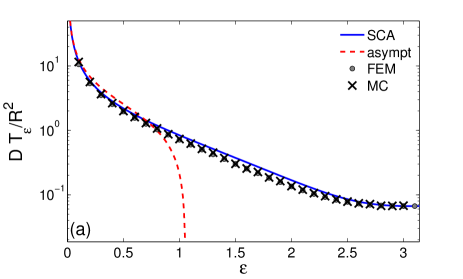
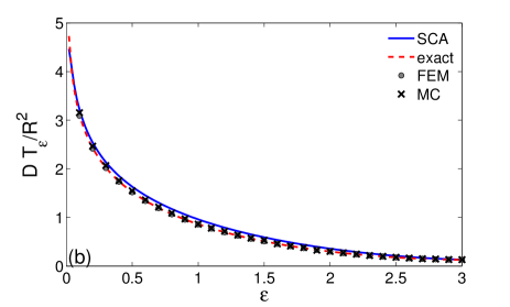
Figure 2: Hard-wall interactions ($U(r)\equiv 0$) and no barrier at the EW ($\kappa=\infty$). The dimensionless global MFET, $DT_{\varepsilon}^{(d)}/R^{2}$, as a function of the target angle $\varepsilon$. (a) 3D Case. Our SCA prediction in (38) and the asymptotic relation in (43) are shown by solid and dashed lines, respectively. The numerical solution by the FEM (with the mesh size $0.01$) is shown by circles, while the Monte Carlo simulations are shown by crosses. (b) 2D Case. Our SCA prediction in (44) (solid line) is compared against the exact result in (47) (dashed line), numerical FEM solution (circles) and MC simulations (crosses).

The first term in (46), which is proportional to $1/\kappa$ and diverges as $1/\varepsilon$ in the limit $\varepsilon\to 0$, is forced to vanish in the idealised case $\kappa\equiv\infty$, and the leading small-$\varepsilon$ behaviour of $T_{\varepsilon}^{(2)}$ in (46) becomes determined by the second term, which exhibits only a slow, logarithmic divergence with $\varepsilon$. At this point it is expedient to recall that the original mixed boundary-value problem in (3) and (4) for the 2D case with $\kappa\equiv\infty$ can be solved exactly Singer06b ; Caginalp12 ; Rupprecht15 and here $T_{\varepsilon}^{(2)}$ reads:

$$T_{\varepsilon}^{(2)} = \frac{R^{2}}{D}\left(\frac{1}{8}-\ln(\sin(\varepsilon/2))\right)$$ (47)

$$= \frac{R^{2}}{D}\ln\left(1/\varepsilon\right)+\dfrac{R^{2}}{D}\left(\ln 2+\dfrac{1}{8}\right)+O\left(\varepsilon^{2}\right).$$

Comparing the solution of the modified problem in (46) with $\kappa\equiv\infty$, and the exact small-$\varepsilon$ expansion in the second line in (47), we conclude that the leading terms in both equations coincide. This means that for the 2D case the SCA developed in the present work determines exactly not only the dependence of the leading term on the pertinent parameters, but also the correct numerical factor. The subdominant, $\varepsilon$-independent term in (46), appears to be slightly larger, by $3/2-2\ln 2\approx 0.114$, than the analogous term in the exact result in (47).

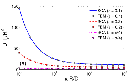
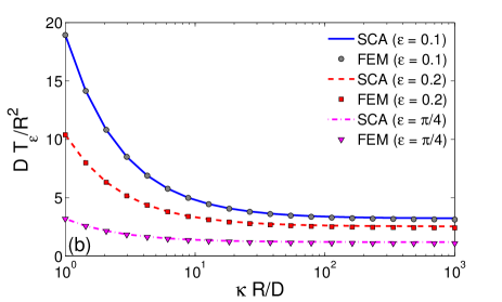
Figure 3: Hard-wall interactions ($U(r)\equiv 0$) with a barrier at the EW. The dimensionless global MFET, $DT_{\varepsilon}^{(d)}/R^{2}$, as a function of a dimensionless parameter $\kappa R/D$ for $\varepsilon=0.1$ (solid line), $\varepsilon=0.2$ (dashed line) and $\varepsilon=\pi/4$ (dotted line): (a) 3D case and (b) 2D case. The SCA (lines) is compared to numerical solutions obtained by a FEM (with the mesh size $0.01$), which are shown by symbols.

Since the SCA is applicable to any size of the EW, we will check its accuracy for the EWs extended beyond the narrow escape limit. As a matter of fact, for chemical reactions involving specific sites localised on the confining boundary, the angular size of the latter is not necessarily small. To this end, in the remaining part of this subsection we will check the $\varepsilon$-dependence of $T_{\varepsilon}$ in (38) and (44) for $\kappa\equiv\infty$, as well as the $\kappa$-dependence of $T_{\varepsilon}$ for fixed $\varepsilon$, and will compare our predictions against the results of numerical simulations (see SM1).

We first consider the well-studied case when there is no barrier at the EW ($\kappa=\infty$), so that the first term in (38) vanishes. Figure 2a compares the SCA prediction in (38), the asymptotic relation (43) by Singer et al. Singer06a , and the numerical solution of the original problem by a finite elements method (FEM) and by Monte Carlo (MC) simulations, which are described in SM1. We observe a fairly good agreement over the whole range of target angles, for $\varepsilon$ varying from $0$ to $\pi$, which is far beyond the narrow escape limit, and the dimensionless parameter $DT_{\varepsilon}/R^{2}$ varying over more than two decades. We find that the SCA provides an accurate solution even for rather large $\varepsilon$, at which the asymptotic relation (43) completely fails. A nearly perfect agreement is also observed for the 2D case (see Fig. 2b).

Next, we study the $\kappa$-dependence of the global MFET. As we have already mentioned, the SCA predicts that the presence of a finite barrier at the entrance to the EW (and hence, for a finite $\kappa$) is fully captured by the first term in (38) and (39). Figure 3 illustrates how accurately the SCA accounts for the effect of a partial reactivity $\kappa$ on the global MFET $T_{\varepsilon}$, even for not too small EW (e.g., for $\varepsilon=\pi/4$) and a broad range of reactivities $\kappa$. For even larger EW, the SCA is still accurate for small $\kappa$ but small deviations are observed at larger $\kappa$ (not shown). As expected, the global MFET diverges as $\kappa\to 0$ because the EW becomes impenetrable, as the remaining part of the boundary is. Similar results are obtained for the 2D case. Overall, we observe a fairly good agreement between our theoretical predictions and the numerical simulations, for both 3D and 2D cases.

IV.2 Global MFET for a system with a triangular-well potential.

We focus on a particular choice of the interaction potential $U(r)$ – a triangular-well radial potential – defined as (see also Fig. S2 in SM4)

$$U(r)=\begin{cases}0,\hskip 59.75078pt0\leq r\leq r_{0},\cr U_{0}\dfrac{r-r_{0}}{R-r_{0}},\qquad r_{0}<r\leq R,\end{cases}$$ (48)

where $0\leq r_{0}\leq R$, $R-r_{0}\equiv l_{ext}$ is the spatial extent of the potential (a characteristic scale) and $U_{0}$ is a dimensionless strength of the potential at the boundary, $U(R)\equiv U_{0}$. Note that $-U_{0}/l_{ext}$ can be interpreted as a constant force exerted on the particle when it appears within a spherical shell of extent $l_{ext}$ near the boundary of the micro-domain. The strength of the potential can be negative (in case of attractive interactions) or positive (in case of repulsive interactions). For this potential, we find explicit closed-form expressions for the radial functions $g_{n}(r)$ (see SM4 and SM5) and examine the dependence of the global MFET on $U_{0}$, $r_{0}$ and other pertinent parameters, such as, $\varepsilon$, $D$, $\kappa$ and $R$.

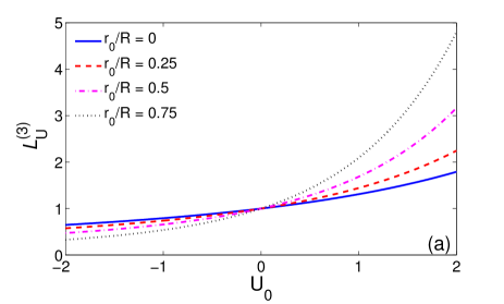
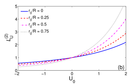
Figure 4: The amplitudes ${\mathcal{L}}^{(3)}_{U}(R)$ (a) and ${\mathcal{L}}^{(2)}_{U}(R)$ (b) in (49) and (50) vs $U_{0}$ for $r_{0}=0$ (solid line), $r_{0}/R=0.25$ (dashed line), $r_{0}/R=0.5$ (dash-dotted line) and $r_{0}/R=0.75$ (dotted line).

We begin with the analysis of the functionals ${\mathcal{L}}^{(3)}_{U}(R)$ and ${\mathcal{L}}^{(2)}_{U}(R)$, which define the amplitudes of all $\varepsilon$-diverging leading terms in (IV) and (35). For the triangular-well potential in (48), these functionals are given explicitly by

$$\begin{array}[]{l}{\mathcal{L}}^{(3)}_{U}(R)=\dfrac{3}{U_{0}^{3}}\biggl{\{}-2-2U_{0}-U_{0}^{2}+(6+4U_{0}+U_{0}^{2})x_{0}\\ -2(3+U_{0})x_{0}^{2}+2x_{0}^{3}+e^{U_{0}}\biggl{[}2+2(U_{0}-3)x_{0}\\ +(6-4U_{0}+U_{0}^{2})x_{0}^{2}-\biggl{(}2-2U_{0}+U_{0}^{2}-\dfrac{U_{0}^{3}}{3}\biggr{)}x_{0}^{3}\biggr{]}\biggr{\}}\,,\\ \end{array}$$ (49)

where $x_{0}=r_{0}/R$, and

$$\begin{array}[]{l}{\mathcal{L}}^{(2)}_{U}(R)=\dfrac{2}{U_{0}^{2}}\biggl{\{}-1-U_{0}+(U_{0}+2)x_{0}-x_{0}^{2}\\ +e^{U_{0}}\biggl{[}1+\left(U_{0}-2\right)x_{0}+\biggl{(}1-U_{0}+\dfrac{U_{0}^{2}}{2}\biggr{)}x_{0}^{2}\biggr{]}\biggr{\}}\,,\\ \end{array}$$ (50)

for the 3D and the 2D cases, respectively. We plot expressions in (49) and (50) in Fig. 4 as functions of $U_{0}$ for different values of $r_{0}$. We observe that for any fixed $r_{0}$, ${\mathcal{L}}^{(3)}_{U}(R)$ and ${\mathcal{L}}^{(2)}_{U}(R)$ are monotonically increasing functions of $U_{0}$, which agrees with the general argument presented earlier in the text. In turn, for any fixed $U_{0}>0$ (repulsive interactions with the boundary), they are increasing functions of $r_{0}$ which means that they are decreasing functions of the extent of the potential, $l_{ext}=R-r_{0}$. Therefore, all the contributions to the global MFET $T_{\varepsilon}$ become larger for stronger repulsion (as they should) and also get increased upon lowering the extent the potential (i.e., upon an increase of the force $-U_{0}/l_{ext}$ pointing towards the bulk and hindering the passage to and through the EW). For sufficiently large positive $U_{0}$ and for any $r_{0}>0$, the dominant contribution to ${\mathcal{L}}^{(d)}_{U}(R)$ is

$${\mathcal{L}}^{(d)}_{U}(R)\sim(r_{0}/R)^{d}\exp(U_{0})\,,\qquad d=2,3\,,$$ (51)

so that the coefficients in the small-$\varepsilon$ expansions of $T_{\varepsilon}$ in (IV) and (35) become exponentially large with $U_{0}$.

In turn, for negative values of $U_{0}$ (attractive interactions), ${\mathcal{L}}^{(3)}_{U}(R)$ and ${\mathcal{L}}^{(2)}_{U}(R)$ decrease upon an increase of $|U_{0}|$ and also decrease when $r_{0}$ approaches $R$, i.e., when the interactions become short ranged.

IV.3 Adam-Delbrück scenario: Limit $\omega=R\,U_{0}/(R-r_{0})\to-\infty$

Before we proceed to the general case with arbitrary $U_{0}$ and $r_{0}$, we discuss first the situations when the dimensionless parameter

$$\omega=R\,U^{\prime}(R)=\frac{R\,U_{0}}{R-r_{0}},$$ (52)

has large negative values. This can be realised for either big negative $U_{0}$, which case is more of a conceptual interest but is apparently not very realistic, or for short-range potentials with fixed $U_{0}<0$ and $r_{0}$ close to $R$, the latter case being physically quite meaningful.

For such values of $\omega$ the leading behaviour of the amplitudes ${\mathcal{L}}^{(3)}_{U}(R)$ and ${\mathcal{L}}^{(2)}_{U}(R)$ is simply described by

$${\mathcal{L}}^{(d)}_{U}(R)\sim\frac{d}{|\omega|}\,,\qquad d=2,3\,,$$ (53)

i.e., the amplitudes vanish as $\omega\to-\infty$ as a first inverse power of $\omega$. This means, in turn, that all the contributions to $T_{\varepsilon}^{(d)}$ which are multiplied by ${\mathcal{L}}^{(d)}_{U}(R)$ (i.e., both the contribution due to a barrier at the EW and the MFPT to the EW) decrease in presence of attractive interactions with the boundary of the micro-domain.

We analyse next the behaviour of another key ingredient of (IV, 35) – the infinite series ${\mathcal{R}}_{\varepsilon}^{(3)}$ and ${\mathcal{R}}_{\varepsilon}^{(2)}$. We realise that there is a subtle point in the behaviour of the latter which stems from the fact that the limit of large negative $\omega$ and the narrow escape limit $\varepsilon\to 0$ do not commute. Taking the limit $\varepsilon\to 0$ first and then turning to the limit $\omega\to-\infty$, we arrive at the expression which describes correctly the behaviour of ${\mathcal{R}}_{\varepsilon}^{(3)}$ and ${\mathcal{R}}_{\varepsilon}^{(2)}$ for small $\varepsilon$ and moderately large $|\omega|$ such that $|\omega|\ll 1/\varepsilon$. If, on contrary, we first take the limit $\omega\to-\infty$ for a fixed $\varepsilon$, and then take the limit $\varepsilon\to 0$, we obtain the correct large-$|\omega|$ behaviour, which yields physically meaningful results for infinitely large negative $\omega$. This point is discussed in detail in SM2.

Accordingly, for the 3D case in the narrow escape limit $\varepsilon\to 0$ with large but finite negative $\omega$, such that $1\ll|\omega|\ll 1/\varepsilon$, we have

$$T^{(3)}_{\varepsilon} \simeq\frac{R^{2}}{D}\biggl{(}\ln(1/\varepsilon)+\ln|\omega|+(\gamma-3/2)\biggr{)}+T_{\pi}^{(3)}(\kappa=\infty)$$

$$+\frac{1}{|\omega|}\left(\frac{4R}{\kappa}\varepsilon^{-2}+\frac{32R^{2}}{3\pi D}\varepsilon^{-1}+O(1)\right)\,,$$ (54)

where $\gamma\approx 0.577$ is the Euler-Mascheroni constant and the MFPT $T_{\pi}^{(3)}(\kappa=\infty)$ from a random location to any point on the boundary is given explicitly for the triangular-well potential by

$$\begin{split}&T_{\pi}^{(3)}(\kappa=\infty)=\frac{r_{0}^{5}}{15DR^{3}}-\frac{R^{2}}{12D\omega}\biggl{(}x_{0}^{4}+3\\ &+\frac{8}{\omega}+\frac{12}{\omega^{2}}-\frac{24}{\omega^{4}}\biggr{)}+\dfrac{R^{2}\,e^{U_{0}}}{3\,D\,\omega}\bigg{(}x_{0}^{3}+\frac{x_{0}^{2}(3-x_{0})}{\omega}\\ &+\frac{3x_{0}(2-x_{0})}{\omega^{2}}+\frac{6(1-x_{0})}{\omega^{3}}-\frac{6}{\omega^{4}}\bigg{)}\,.\end{split}$$ (55)

Note that in the limit $\omega\to-\infty$, the MFPT $T_{\pi}^{(3)}(\kappa=\infty)$ becomes

$$T_{\pi}^{(3)}(\kappa=\infty)=\frac{r_{0}^{5}}{15DR^{3}}+O\left(\frac{1}{|\omega|}\right)\,,$$ (56)

where the leading in this limit term can be interpreted as the product of the probability $(r_{0}/R)^{3}$ that the particle’s starting point is within the spherical region of radius $r_{0}$ (in which diffusion is not influenced by the potential), and the MFPT, equal to $r_{0}^{2}/(15D)$, from a random location within this spherical region to its boundary. Clearly, when a particle reaches the extent of the infinitely strong attractive potential (or if it was started in that region), it is drifted immediately to the boundary, and this step does not increase the MFPT.

On the other hand, for small $\varepsilon$ and negative $\omega$ which can be arbitrarily (even infinitely) large by an absolute value, we find (see SM2)

$$T^{(3)}_{\varepsilon} \simeq\frac{R^{2}}{D}\biggl{(}2\,\ln(1/\varepsilon)+\ln 2-1/4\biggr{)}+T_{\pi}^{(3)}(\kappa=\infty)$$

$$+\frac{1}{|\omega|}\left(\frac{4R}{\kappa}\varepsilon^{-2}+O(1)\right)\,,$$ (57)

which differs from the expression in (IV.3) in two aspects: the amplitude of the dominant term, which diverges logarithmically as $\varepsilon\to 0$, is twice larger, and the term $\ln|\omega|$, which diverges logarithmically as $\omega\to-\infty$, is absent.

Therefore, we observe that attractive interactions with either large negative $U_{0}$, or fixed negative $U_{0}$ and $r_{0}\sim R$ (both giving a large negative $\omega$ according to (52)), effectively suppress the contribution due to a finite barrier at the entrance to the EW, and also the contribution due to the diffusive paths which find the EW via 3D diffusion. On contrary, such interactions do not affect the term which is logarithmically diverging as $\varepsilon\to 0$ and is associated with the paths localised near the confining boundary. In other words, in this limit the plausible scenario to find the EW is that of the dimensionality reduction, suggested by Adam and Delbrück adam : a particle diffuses in the bulk until it hits the confining boundary at some random position (which takes time of order of $r_{0}^{5}/(15DR^{3})$, see the first term in (55)), and then diffuses along the boundary, not being able to surmount the barrier against desorption and to escape back to the bulk, until it ultimately finds the EW (the term $2R^{2}\ln(1/\varepsilon)/D$).

It is worthwhile to mention that our SCA approach reproduces the leading in the limit $\varepsilon\to 0$ behaviour of the MFPT due to the surface diffusion exactly, i.e., not only the $\varepsilon$-dependence but also the numerical factor in the amplitude. In fact, the mean time $T_{s}$ needed for a particle, diffusing on a surface of a 3D sphere and starting at a random point, to arrive for the first time to a disc of an angular size $\varepsilon$ located on the surface of this sphere has been calculated exactlySano79 :

$$T_{s} = \frac{R^{2}}{D}\left(\ln\left(\frac{2}{1-\cos\varepsilon}\right)-\frac{1+\cos\varepsilon}{2}\right)$$ (58)

$$\simeq \frac{R^{2}}{D}\biggl{(}2\ln(1/\varepsilon)+2\ln 2-1+O(\varepsilon^{2})\biggr{)}.$$ (59)

Comparing (IV.3) and (59), we notice that the leading terms in both expressions are identical, and that both expressions differ slightly only by numerical constants in the $\varepsilon$-independent terms.

In the 2D case with large negative $\omega$, the dominant contribution to the MFET comes not from the logarithmically diverging term in the limit $\varepsilon\to 0$, as one could expect, but rather from the infinite sum in the second line in (IV), which is independent of $\varepsilon$. We discuss this observation in SM2 and show that this sum diverges in proportion to $|\omega|$ when $\omega\to-\infty$. Using the asymptotic relation (S60), which presents this contribution to ${\mathcal{R}}_{\varepsilon}^{(2)}$ in an explicit form, we find

$$\begin{split}T^{(2)}_{\varepsilon}&=T_{\pi}^{(2)}(\kappa=\infty)+\frac{\pi^{2}R^{2}}{3D}+O(1)\\ &+\frac{1}{|\omega|}\left(\dfrac{\pi R}{\kappa}\,\varepsilon^{-1}+\dfrac{2R^{2}}{D}\,\ln(1/\varepsilon)\right)\,,\\ \end{split}$$ (60)

where $T_{\pi}^{(2)}(\kappa=\infty)$ is the MFPT from a random location within the disc to any point on its boundary. For the triangular-well potential the latter is given explicitly by

$$T_{\pi}^{(2)}(\kappa=\infty)=\frac{r_{0}^{4}}{8DR^{2}}-\frac{R^{2}}{6D\omega}\biggl{(}x_{0}^{3}+2+\frac{3}{\omega}-\frac{6}{\omega^{3}}\biggr{)}$$

$$+\frac{R^{2}\,e^{U_{0}}}{2\,D\,\omega}\biggl{(}x_{0}^{2}+\frac{x_{0}(2-x_{0})}{\omega}+\frac{2(1-x_{0})}{\omega^{2}}-\frac{2}{\omega^{3}}\biggr{)}\,.$$ (61)

For large negative $\omega$, the leading term in (IV.3) is $r_{0}^{4}/(8DR^{2})$. This term can be simply interpreted as the mean time, equal to $r_{0}^{2}/(8D)$, needed to appear for the first time within the reach of the triangular-well potential for a particle whose starting point is uniformly distributed within the subregion $r<r_{0}$ (in which diffusion is free), multiplied by the probability $r_{0}^{2}/R^{2}$ that this starting point is within this subregion.

Hence, in the limit $\omega\to-\infty$, we obtain for the 2D case

$$T^{(2)}_{\varepsilon}\approx\left(\frac{r_{0}}{R}\right)^{2}\,\frac{r_{0}^{2}}{8D}+\frac{\pi^{2}R^{2}}{3D}\,.$$ (62)

Again, we observe that the contribution due to a barrier at the EW, and the leading, logarithmically divergent contribution to the MFPT to the EW due to a two-dimensional diffusive search within the disc, are both suppressed by attractive interactions. Indeed, in this case a plausible Adam-Delbrück-type argument adam states that a diffusive particle first finds the boundary of the disc (the first term in (62)), and then diffuses along the boundary until it ultimately finds the EW. For arbitrary $\varepsilon$ the latter MFPT is well-known and is given by

$$T_{s}=\frac{R^{2}}{D}~{}\frac{(\pi-\varepsilon)^{3}}{3\pi}=\frac{\pi^{2}R^{2}}{3D}+O(\varepsilon)\,,$$ (63)

where the leading term on the right-hand-side is exactly the same as the second term in (62). This implies that our SCA approach predicts correctly the values of both MFPTs.

To summarise the results of this subsection, we note that the behaviour observed in the limit $\omega\to-\infty$ follows precisely the Adam-Delbrück dimensionality reduction scenario for both 3D and 2D cases. Our expressions (IV.3) and (60) provide the corresponding MFETs, and also define the correction terms due to finite values of $\omega$. We emphasise, however, that the limit $\omega\to-\infty$ is an extreme case. For modest negative $\omega$ the representative trajectories for both three-dimensional and two-dimensions systems will consist of paths of alternating phases of bulk diffusion and diffusion along the boundary. We analyse this situation below.

IV.4 Beyond the Adam-Delbrück scenario: Arbitrary $U_{0}$ and $r_{0}$.

Consider the behaviour of the global MFET defined in (IV) or (35) for arbitrary $U_{0}$ and $r_{0}$. Taking into account the explicit expressions for ${\mathcal{L}}^{(3)}_{U}(R)$ in (49) and for ${\mathcal{L}}^{(2)}_{U}(R)$ in (50), we notice that the coefficients in front of each term in (IV) and (35) are monotonic functions of $U_{0}$ . This implies that in the narrow escape limit $\varepsilon\to 0$, we do not expect any non-monotonic behaviour of the global MFET with respect to $U_{0}$. A thorough analytical and numerical analysis of $T_{\varepsilon}^{(d)}$ shows that it is indeed the case.

As we expected on intuitive grounds, for attractive particle-boundary interactions the global MFET $T_{\varepsilon}^{(d)}$ appears to be a non-monotonic, and hence, an optimisable function of the extent of the potential. This is a new spectacular feature of the NEP unveiled by our model involving spatially-extended interactions with the confining boundary. In Figs. 5a and 5b we plot $T_{\varepsilon}^{(3)}$ and $T_{\varepsilon}^{(2)}$, defined by (IV) and (35) with $\kappa=\infty$, as a function of $r_{0}$ for several negative values of $U_{0}$ ($U_{0}=-1$, $U_{0}=-2$ and $U_{0}=-5$) and $\varepsilon=0.02$. We remark that the first terms in (IV) and (35), associated with a finite barrier and dropped by setting $\kappa=\infty$, are monotonic functions of $r_{0}$.

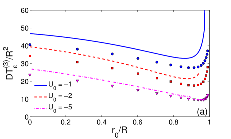
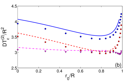
Figure 5: The dimensionless global MFET, $DT^{(d)}_{\varepsilon}/R^{2}$, as a function of $x_{0}=r_{0}/R$ for a triangular-well potential with no barrier at the EW, $\kappa=\infty$. Our analytical predictions are shown by curves for three values of $U_{0}$ and $\varepsilon=0.02$. Symbols present numerical solutions obtained by a FEM (with the mesh size $0.005$). (a) 3D case, $T^{(3)}_{\varepsilon}$ is given by (IV); (b) 2D case, $T^{(2)}_{\varepsilon}$ is given by (35).

We observe that in the 3D case, the global MFET $T_{\varepsilon}^{(3)}$, as a function of $r_{0}$, exhibits a rather pronounced minimum for $r_{0}$ away from $r_{0}=0$ and from $r_{0}=R$ (contact interactions). This means that there exists an optimal extent of the potential: in order to minimise the global MFET, the potential should neither extend too deep into the bulk nor should be too localised on the boundary. Further on, we realise that the precise location of the minimum of $T_{\varepsilon}^{(3)}$ depends, in general, on $\varepsilon$ and $U_{0}$. Analysing our result in (IV), we observe that when we gradually decrease $\varepsilon$, the minimum moves closer to the boundary (but never reaches it and $T_{\varepsilon}^{(3)}$ still exhibits a very abrupt growth when $r_{0}$ becomes too close to $R$) and becomes more pronounced. Conversely, if we progressively increase $\varepsilon$, the minimum moves away from the boundary and becomes more shallow. Increasing the strength of attractive interactions (while keeping $\varepsilon$ fixed) also pushes the minimum closer to the boundary.

For the 2D case the global MFET $T_{\varepsilon}^{(2)}$ shows a qualitatively similar behaviour but the effects are much less pronounced. In principle, the optimum also exists in this case, but the minimum appears to be much more shallow. We also observe that for strong attraction ($U_{0}=-5$), apart of some deep in the vicinity of $r_{0}=R$, $T_{\varepsilon}^{(2)}$ appears to be almost independent of $r_{0}$.

As in the analysis of the NEP without the particle-boundary interactions in Sec. IV.1, one can observe some small discrepancies between the asymptotic relations (IV, 35) and numerical solutions of the original problem by a FEM. As discussed earlier, they are related to the SCA approximation, in which the mixed boundary condition is replaced by an effective inhomogeneous Neumann condition. On the other hand, the proposed approximation provides explicit asymptotic formulae for arbitrary potentials that captures qualitatively well all the studied features of the NEP.

Two remarks are now in order:

a) Emergence of an optimum at an intermediate extent of the potential implies that the Adam-Delbrück dimensionality reduction scenario (which corresponds to $\omega\to-\infty$ and hence, to the part of the curves in Figs. 5a and 5b close to $r_{0}=R$ where $T_{\varepsilon}^{(3)}$ exhibits quite a steep growth attaining large values) is not at all the optimal (i.e., less time consuming) way of finding the EW. In reality, the optimum corresponds to situations when the barrier against desorption is not very large so that the particle does not remain localised near the boundary upon approaching it for the first time, but rather has a possibility to overpass the barrier against desorption and to perform alternating phases of bulk and surface diffusion. The optimum then corresponds to some fine-tuning of the relative weights of bulk and surface diffusion by changing the extent of the potential and its value on the boundary.

b) These findings are compatible, in principle, with the prediction of the non-monotonic behaviour of $T_{\varepsilon}^{(d)}$ as a function of the desorption rate $\lambda$ made earlier in greb2 , in which the NEP with $\kappa=\infty$ has been analysed for an intermittent diffusion model. In this model a particle diffuses in the bulk with a diffusion coefficient $D$ until it hits the boundary of the micro-domain and switches to surface diffusion of a random duration (controlled by the desorption rate $\lambda$) with a diffusion coefficient $D_{\rm surf}$. This model tacitly presumes that there are some attractive interactions with the surface, in addition to the hard-core repulsion, which are taken into account in some effective way (interactions are replaced by effective contact ones). In our settings, the desorption rate $\lambda$ in this intermittent model should depend on both the strength of the interaction potential $U_{0}$ at the boundary and also on the gradient of the potential in the vicinity of the surface, which define the barrier against desorption. There is, however, some quantitative discrepancy between our predictions and the predictions made in greb2 : In greb2 (see Fig. 10, right panel), it was argued that for such an intermittent model with $D=D_{\rm surf}$ (as in our case) surface diffusion is a preferable search mechanism so that the global MFET is a monotonic function of $\lambda$. On contrary, our analysis demonstrates that $T_{\varepsilon}^{(3)}$ is an optimisable function even in case of equal bulk and surface diffusion coefficients, which means that neither the bulk diffusion nor 2D surface diffusion alone provide an optimal search mechanism, but rather their combination. This discrepancy is related to subtle differences between two models. For the two-dimensional case, illustrated in Fig. 5b, the analysis in greb2 (see Fig. 10, left panel) suggests that there is an optimum even for $D=D_{\rm surf}$. Our analysis agrees with this conclusion.

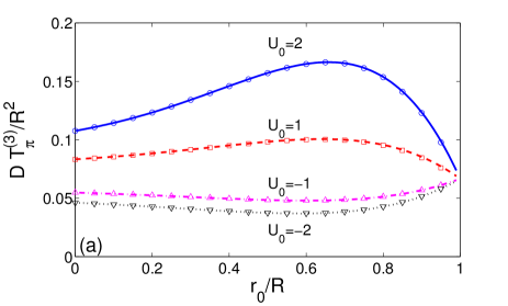
Figure 6: The dimensionless MFPT, $DT^{(d)}_{\pi}(\kappa=\infty)/R^{2}$, for a triangular-well potential in (48) versus $r_{0}/R$ for several values of $U_{0}$ and $\kappa=\infty$. (a) 3D case, (b) 2D case.

We close with a brief analysis of the behaviour of $T_{\pi}^{(d)}(\kappa=\infty)$ – the MFPT for a diffusive particle, starting at a random location, to arrive at any point on the boundary of the micro-domain, in presence of long-range interactions with the boundary. This MFPT is included into $T_{\varepsilon}^{(d)}$ but has a little effect on it since it enters only the constant, $\varepsilon$-independent terms. At the same time, it is an interesting quantity in its own right. For the triangular-well potential, $T_{\pi}^{(d)}(\kappa=\infty)$ is defined explicitly by (55) and (IV.3) for $d=3$ and $d=2$, respectively.

A first intuitive guess is that increasing either $U_{0}$ or the extent of the potential would make the particle feel the surface stronger, so that for $U_{0}>0$, the MFPT $T_{\pi}^{(d)}(\kappa=\infty)$ would be an increasing function of both parameters, while for $U_{0}<0$, $T_{\pi}^{(d)}(\kappa=\infty)$ would decrease with an increase of both $U_{0}$ and $r_{0}$. As far as the dependence on $U_{0}$ is concerned, this guess appears to be correct. Indeed, we observe that for a fixed $r_{0}$, the MFPTs for both $d=2$ and $d=3$ are monotonic increasing functions of $U_{0}$. Surprisingly enough, this is not the case for the dependence of the MFPTs $T_{\pi}^{(d)}(\kappa=\infty)$ on the extent $l_{ext}$ of the potential. We find that for a fixed $U_{0}$, $T_{\pi}^{(d)}(\kappa=\infty)$ exhibits a peculiar non-monotonic behaviour as a function of $r_{0}$, with a minimum for $U_{0}<0$ and a maximum for $U_{0}>0$, as illustrated in Fig. 6. To the best of our knowledge, this interesting effect has not been reported earlier.

V Conclusion

To recapitulate, we have presented here some new insights into the narrow escape problem, which concerns various situations when a particle, diffusing within a bounded micro-domain, has to escape from it through a small window (or to bind to some target site) of an angular size $\varepsilon$ located on the impenetrable boundary. We have focused on two aspects of this important problem which had not received much attention in the past: the effects of an energy or an entropy barrier at the escape window, always present in realistic systems, and the effects of long-range potential interactions between a diffusing particle and the boundary. Inspired by the self-consistent approximation developed previously in shoup for calculation of the reaction rates between molecules with inhomogeneous chemical reactivity, we generalised this approach to the NEP with long-range potential interactions with the boundary. In this self-consistent approach, the original mixed boundary condition is replaced by an effective inhomogeneous Neumann condition, in which the unknown flux is determined from an appropriate closure relation. This modified problem was solved exactly for an arbitrary radial interaction potential.

We have concentrated on the functional form of the global (or volume-averaged over the starting point) mean first exit time, $T_{\varepsilon}$, for which we derived a general expression analogous to the celebrated Collins-Kimball relation in chemical kinetics, incorporating both the contribution due to a finite barrier at the escape window (or a binding site) and the contribution due to a diffusive search for its location, for an arbitrary radially-symmetric potential, any size of the escape window, and a barrier of an arbitrary height. We have realised that these two contributions naturally decouple from each other, which permitted us to study separately their impact on the MFET.

The accuracy of our analytical results based on the self-consistent approximation has been confirmed by two independent numerical schemes: a numerical solution of the backward Fokker-Planck equation by a finite element method, and Monte Carlo simulations of the diffusive search for the escape window in presence of particle-boundary potential interactions. We have shown that the self-consistent approximation is very accurate for small escape windows (i.e., in the true narrow escape limit) but also captures quite well the behaviour of the global MFET even for rather large escape windows. In the latter case, small deviations were observed, related to the fact that the solution of the modified problem is defined up to a constant.

Turning to the narrow escape limit $\varepsilon\to 0$, we have analysed the relative weights of each contribution to $T_{\varepsilon}$. We have shown that the contribution due to the passage through the escape window (which had been ignored in the majority of earlier works) dominates the global MFET in the narrow escape limit, since it exhibits a stronger singularity as $\varepsilon\to 0$ than the contribution due to the diffusive search. This implies that the kinetics of the narrow escape process is rather barrier-controlled than diffusion-controlled. In consequence, discarding an entropy or an energy barrier at the exit from the micro-domain can result in strongly misleading estimates in chemical and biological applications. Remarkably, the associated reactivity (or permeability) enters into the global MFET in a very simple way.

Further on, for the case of radially-symmetric interaction potentials which possess a bounded first derivative, we have presented an explicit expression for the contribution to $T_{\varepsilon}$ due to the diffusive search for the location of the escape window, in which the coefficients in front of the terms diverging in the limit $\varepsilon\to 0$ were defined via some integrals and derivatives of the interaction potential. The structure of the obtained result suggests that most likely the general problem considered here can be solved exactly in the narrow escape limit without resorting to any approximation.

On example of a triangular-well interaction potential, we have discussed the dependence of the contribution to the MFET due to a diffusive search for the escape window on the parameters of the potential. We have shown that this contribution is always a monotonic function of the value of the potential at the boundary: as expected, repulsive (resp., attractive) interactions increase (resp., decrease) the MFET. Curiously enough, it appeared that for attractive interactions $T_{\varepsilon}$ is a non-monotonic function of the extent of the potential: there exists some optimal extent for which $T_{\varepsilon}$ has a minimum. This optimal value corresponds to interactions which are neither localised near the confining boundary nor extend to deeply into the bulk. In case of a very small extent (i.e., in the limit of short-range interactions), with a fixed value of the interactions potential on the boundary, the force acting on the particle in the immediate vicinity of the boundary becomes very large and the narrow escape process proceeds precisely via the Adam-Delbrück dimensionality reduction scenario: a particle first reaches the boundary at any point and than, not being able to surmount the barrier against desorption, continues a diffusive search for the escape window along the boundary until it finds it. For more realistic moderate values of the extent, typical paths consist of alternating, intermittent bulk diffusion tours followed by diffusion along the boundary.

Supplemental Materials

SM1 Numerical simulations

In this part of the Supplemental Materials we briefly discuss two numerical procedures used to check our theoretical predictions.

SM1.1 Numerical computation by a finite elements method

To verify the accuracy of the SCA, we solve the Poisson equation (2, 3) by using a finite elements method (FEM) implemented in Matlab PDEtool. This tool solves the following equation:

$$-\nabla(c\nabla u)+au=f,$$ (S1)

where $c$ is a 2x2 matrix, and $a$ and $f$ are given functions.

In our case, we need to deal with the Laplace operator in radial or spherical coordinates. In two dimensions, the original equation (3) can be written in radial coordinates as

$$\frac{1}{r}\partial_{r}(re^{-U(r)}\partial_{r})u+\frac{e^{-U(r)}}{r^{2}}\partial^{2}_{\theta}u=-\frac{e^{-U(r)}}{D},$$ (S2)

from which

$$-\left(\begin{array}[]{c}\partial_{r}\\ \partial_{\theta}\\ \end{array}\right)^{\dagger}c\left(\begin{array}[]{c}\partial_{r}\\ \partial_{\theta}\\ \end{array}\right)u=f,$$ (S3)

with $a=0$, $f=re^{-U(r)}/D$, and

$$c=\left(\begin{array}[]{c c}re^{-U(r)}&0\\ 0&e^{-U(r)}/r\\ \end{array}\right).$$ (S4)

In three dimensions, the Poisson equation (2) reads in spherical coordinates as

$$\frac{1}{r^{2}}\partial_{r}(r^{2}e^{-U(r)}\partial_{r})u+\frac{e^{-U(r)}}{r^{2}}\frac{1}{\sin\theta}\partial_{\theta}(\sin\theta\partial_{\theta})u$$

$$+\frac{e^{-U(r)}}{r^{2}\sin^{2}\theta}\partial^{2}_{\varphi}u=-\frac{e^{-U(r)}}{D}.$$ (S5)

Since our solution does not depend on $\varphi$, the last term on the left hand side can be omitted so that

$$-\left(\begin{array}[]{c}\partial_{r}\\ \partial_{\theta}\\ \end{array}\right)^{\dagger}c\left(\begin{array}[]{c}\partial_{r}\\ \partial_{\theta}\\ \end{array}\right)u=f,$$ (S6)

with $a=0$, $f=r^{2}e^{-U(r)}\sin\theta/D$, and

$$c=\left(\begin{array}[]{c c}r^{2}e^{-U(r)}\sin\theta&0\\ 0&e^{-U(r)}\sin\theta\\ \end{array}\right).$$ (S7)

We set the rectangular domain $V=[0,1]\times[0,\pi]$ with mixed boundary conditions (4), i.e., a zero flux condition for $\partial V\backslash\Gamma_{0}$, except for the segment $\Gamma_{0}=\{1\}\times[0,\varepsilon]$ representing the EW (see Fig. S1):

$$\begin{split}\biggl{(}\partial_{r}u+\frac{k}{D}u\biggr{)}_{r=1}&=0\qquad(\textrm{on}~{}\Gamma_{0}),\\ (\partial_{r}u)_{r=1}&=0\qquad(\textrm{on}~{}\Gamma_{1}),\\ (\partial_{r}u)_{r=0}&=0\qquad(\textrm{on}~{}\Gamma_{3}),\\ (\partial_{\theta}u)_{\theta=0}&=0\qquad(\textrm{on}~{}\Gamma_{4}),\\ (\partial_{\theta}u)_{\theta=\pi}&=0\qquad(\textrm{on}~{}\Gamma_{2}).\\ \end{split}$$ (S8)

In Matlab, the generalised Neumann boundary condition has the form

$$\vec{n}\cdot(c\nabla u)+qu=g,$$ (S9)

where the matrix $c$ is the same as in the PDE (S1). We set $g=0$ and

$$\begin{split}q&=Re^{-U(R)}\kappa/D\qquad(\textrm{on}~{}\Gamma_{0}),\\ q&=0\qquad(\textrm{on}~{}\Gamma_{1}\cup\Gamma_{2}\cup\Gamma_{3}\cup\Gamma_{4})\\ \end{split}$$ (S10)

in two dimensions, and

$$\begin{split}q&=R^{2}\sin\theta~{}e^{-U(R)}\kappa/D\qquad(\textrm{on}~{}\Gamma_{0}),\\ q&=0\qquad(\textrm{on}~{}\Gamma_{1}\cup\Gamma_{2}\cup\Gamma_{3}\cup\Gamma_{4})\\ \end{split}$$ (S11)

in three dimensions. For fully reactive EW ($\kappa=\infty$), the Dirichlet boundary condition is imposed on $\Gamma_{0}$.

Figure S1: The original domain (half-disc) and the associated computational domain (rectangle). Similar in 3D case.

SM1.2 Monte Carlo simulations

We also compute the distribution of first passage times to the EW by simulating diffusion trajectories which end up at the EW. In practice, we solve a Langevin equation by the following iterative procedure: after generating a uniformly distributed starting point ${\bf r}_{0}$, one re-iterates

$${\bf r}_{n+1}={\bf r}_{n}+D\delta~{}{\bf f}({\bf r}_{n})+\sqrt{2D\delta}~{}\xi_{n}\,,$$ (S12)

where $\delta$ is a one-step duration, ${\bf r}_{n}$ is the position after $n$ steps, ${\bf f}=-\partial_{r}U(r){\bf e}_{r}$ is the normalised applied force in the radial direction ${\bf e}_{r}$, and $\xi$ is the normalised random thermal force. For instance, we have in two dimensions:

$$\begin{split}x_{n+1}&=x_{n}+D\delta~{}f(|{\bf r}_{n}|)~{}x_{n}/|{\bf r}_{n}|+\sqrt{2D\delta}~{}\xi_{x,n}\,,\\ y_{n+1}&=y_{n}+D\delta~{}f(|{\bf r}_{n}|)~{}y_{n}/|{\bf r}_{n}|+\sqrt{2D\delta}~{}\xi_{y,n}\,,\\ \end{split}$$ (S13)

where $x_{n}/|{\bf r}_{n}|$ and $y_{n}/|{\bf r}_{n}|$ represent $\cos(\theta)$ and $\sin(\theta)$ in the projection of the radial force, and $\xi_{x,n}$, $\xi_{y,n}$ are independent normal variables with zero mean and unit variance.

At each step, one checks whether the new position $(x_{n+1},y_{n+1})$ remains inside the disk: $x_{n+1}^{2}+y_{n+1}^{2}<R^{2}$. If this condition is not satisfied, the particle is considered as being on the boundary. If the particle hits the EW, the trajectory simulation is stopped and $n\delta$ is recorded as the generated exit time. Otherwise, the particle is reflected back and continues to diffuse. The Monte Carlo simulations in three dimensions are similar. Finally, the partial reactivity of the EW can be introduced by partial reflections Grebenkov06 ; Grebenkov14 .

SM2 Asymptotic behaviour of the series in (19) and (24)

We focus on the asymptotic behaviour of the infinite series ${\mathcal{R}}_{\varepsilon}^{(3)}$ and ${\mathcal{R}}_{\varepsilon}^{(2)}$, defined in (19) and (24), for potentials $U(r)$ which have a bounded first derivative for any $r\in(0,R)$. Our aims here are two-fold: first we establish the exact asymptotic expansions for these infinite series in the narrow escape limit $\varepsilon\to 0$, and second, we derive approximate explicit expressions for ${\mathcal{R}}_{\varepsilon}^{(3)}$ and ${\mathcal{R}}_{\varepsilon}^{(2)}$ which permit us to investigate their asymptotic behaviour in the limit $R|U^{\prime}(R)|\to\infty$.

Our analysis is based on two complementary approaches. In the first approach we take advantage of the following observation. When $\varepsilon=0$, there is no EW, and the MFET is infinite, whatever the potential is. Since ${\mathcal{L}}_{U}^{(d)}$ does not depend on $\varepsilon$, the divergence of the MFET as $\varepsilon\to 0$ should be ensured by the divergence of ${\mathcal{R}}_{\varepsilon}^{(d)}$. Suppose that we truncate the infinite series in (19) and (24) at some arbitrary $n=N^{*}$. Then, turning to the limit $\varepsilon\to 0$, we find that both ${\mathcal{R}}_{\varepsilon}^{(3)}$ and ${\mathcal{R}}_{\varepsilon}^{(2)}$ attain some constant values, which depend on the upper limit $N^{*}$ of summation. As a consequence, these truncated sums should diverge as $N^{*}\to\infty$ while their small-$\varepsilon$ behaviour is dominated by the terms with $n\to\infty$. One needs therefore to determine the asymptotic behaviour of $g_{n}(R)/g^{\prime}_{n}(R)$ in this limit and to evaluate the corresponding small-$\varepsilon$ asymptotics for ${\mathcal{R}}_{\varepsilon}^{(3)}$ and ${\mathcal{R}}_{\varepsilon}^{(2)}$. This will be done in the subsection SM2.1.

Next, in subsection SM2.2 we will pursue a different approach based on the assumption that, once we are interested in the behaviour of the ratio $g_{n}/g^{\prime}_{n}$ at $r=R$ only, we may approximate the coefficients in the differential equations (7) and (20), which are functions of $r$, by taking their values at the confining boundary. This will permit us to derive an explicit expression for $g_{n}(R)/g^{\prime}_{n}(R)$ valid for arbitrary $n$, not necessarily large, and arbitrary $|U^{\prime}(R)|<\infty$. This expression will be checked subsequently against an exact solution obtained for a triangular-well potential (see SM4 and SM5). We set out to show that an approximate expression for $g_{n}(R)/g^{\prime}_{n}(R)$ and an exact result for such a choice of the potential agree very well already for quite modest values of $n$ and the agreement becomes progressively better with an increase of $|U^{\prime}(R)|$. On this basis, we also determine the small-$\varepsilon$, as well large-$RU^{\prime}(R)$ asymptotic behaviour of ${\mathcal{R}}_{\varepsilon}^{(3)}$ and ${\mathcal{R}}_{\varepsilon}^{(2)}$, which agrees remarkably well with the expressions obtained within the first approach, and the exact solution derived for the particular case of a triangular-well potential.

SM2.1 Large-$n$ asymptotics of $g_{n}(R)/g^{\prime}_{n}(R)$ and the corresponding small-$\varepsilon$ behaviour of the infinite series ${\mathcal{R}}_{\varepsilon}^{(3)}$ and ${\mathcal{R}}_{\varepsilon}^{(2)}$.

We introduce an auxiliary function $\psi=\psi_{n}(r)=g_{n}(r)/g^{\prime}_{n}(r)$, which is the inverse of the logarithmic derivative of $g_{n}(r)$ and obeys, in virtue of (7) and (20), the following equations:

$$r^{2}\left(1-\psi^{\prime}\right)+r\left(2-rU^{\prime}(r)\right)\psi-n(n+1)\psi^{2}=0$$ (S14)

for the 3D case, and

$$r^{2}\left(1-\psi^{\prime}\right)+r\left(1-rU^{\prime}(r)\right)\psi-n^{2}\psi^{2}=0$$ (S15)

for the 2D case, respectively. We will seek the solutions of these non-linear Riccati-type differential equations in form of the asymptotic expansion in the inverse powers of $n$ in the limit $n\to\infty$.

Supposing that $U^{\prime}(r)$ does not diverge at any point within the domain, we find that the leading term of $\psi$ in the limit $n\to\infty$ is given by $\psi\sim r/n$ for both 2D and 3D cases, which is completely independent of the potential $U(r)$. Pursuing this approach further, we make no other assumption to get the second term in this large-$n$ expansion, while for the evaluation of the third term we stipulate that $|U^{\prime\prime}(r)|<\infty$. We have then for the 3D case

$$\psi=\frac{r}{n}-\frac{r^{2}U^{\prime}(r)}{2n^{2}}+\frac{r^{2}\left(U^{\prime}(r)\left(4+r\,U^{\prime}(r)\right)+2\,r\,U^{\prime\prime}(r)\right)}{8n^{3}}+O\left(\frac{1}{n^{4}}\right)\,,$$ (S16)

and hence,

$$\frac{g_{n}(R)}{Rg^{\prime}_{n}(R)}=\frac{1}{n}-\frac{RU^{\prime}(R)}{2n^{2}}+\frac{RU^{\prime}(R)\left(4+R\,U^{\prime}(R)\right)+2\,R^{2}\,U^{\prime\prime}(R)}{8n^{3}}+O\left(\frac{1}{n^{4}}\right)\,,$$ (S17)

where the omitted terms decay in the leading order as $1/n^{4}$. Similarly, for the 2D case we find

$$\psi=\frac{r}{n}-\frac{r^{2}U^{\prime}(r)}{2n^{2}}+\frac{r^{2}\left(U^{\prime}(r)\left(2+r\,U^{\prime}(r)\right)+2\,r\,U^{\prime\prime}(r)\right)}{8n^{3}}+O\left(\frac{1}{n^{4}}\right)\,,$$ (S18)

and hence,

$$\frac{g_{n}(R)}{Rg^{\prime}_{n}(R)}=\frac{1}{n}-\frac{RU^{\prime}(R)}{2n^{2}}+\frac{RU^{\prime}(R)\left(2+R\,U^{\prime}(R)\right)+2\,R^{2}\,U^{\prime\prime}(R)}{8n^{3}}+O\left(\frac{1}{n^{4}}\right)\,.$$ (S19)

We observe that the asymptotic expansions (S17) and (S19) for the 3D and the 2D cases become different from each other only starting from the third term; first two terms are exactly the same. As it will be made clear below, we do not have to proceed further with this expansion and, as an actual fact, just two first terms will suffice us to determine the leading asymptotic behaviour of ${\mathcal{R}}_{\varepsilon}^{(3)}$ and just the first one will be enough to determine the analogous behaviour of ${\mathcal{R}}_{\varepsilon}^{(2)}$. In what follows, in SM4 and SM5 we will also check these expansions against the exact results obtained for the triangular-well potential, in which case the radial functions $g_{n}$ and hence, the ratio $g_{n}(R)/g^{\prime}_{n}(R)$ can be calculated exactly. We proceed to show that the asymptotic forms in (S17) and (S19) coincide with the exact asymptotic expansions at least for the first three terms.

Focusing first on the 3D case, we formally write

$$\frac{g_{n}(R)}{Rg^{\prime}_{n}(R)}\equiv\frac{1}{n}-\frac{R\,U^{\prime}(R)}{2n^{2}}+\left(\frac{g_{n}(R)}{Rg^{\prime}_{n}(R)}-\frac{1}{n}+\frac{R\,U^{\prime}(R)}{2n^{2}}\right)\,,$$ (S20)

where the terms in brackets, in virtue of (S16) and (S17), decay as $1/n^{3}$ when $n\to\infty$. Inserting (S20) into (19), we have

$${\mathcal{R}}_{\varepsilon}^{(3)} =\Sigma_{1}-R\,U^{\prime}(R)\,\Sigma_{2}+\sum\limits_{n=1}^{\infty}\left(\frac{g_{n}(R)}{Rg^{\prime}_{n}(R)}-\frac{1}{n}+\frac{RU^{\prime}(R)}{2n^{2}}\right)\frac{\phi_{n}^{2}(\varepsilon)}{(2n+1)}\,,$$ (S21)

where

$$\Sigma_{1} =\sum\limits_{n=1}^{\infty}\frac{\phi_{n}^{2}(\varepsilon)}{n(2n+1)},$$ (S22)

$$\Sigma_{2} =\frac{1}{2}\sum_{n=1}^{\infty}\frac{\phi_{n}^{2}(\varepsilon)}{n^{2}(2n+1)}\,,$$ (S23)

and $\phi_{n}(\varepsilon)$ is defined by (15).

Next, we find that in the limit $\varepsilon\to 0$,

$$\Sigma_{1}=\frac{32}{3\pi}\varepsilon^{-1}+\ln\left(1/\varepsilon\right)-\frac{7}{4}+\ln 2+O(\varepsilon)\,,$$ (S26)

$$\Sigma_{2}=\ln\left(1/\varepsilon\right)+\frac{1}{4}+\ln 2+\frac{\pi^{2}}{12}+O(\varepsilon)\,,$$

$$\sum\limits_{n=1}^{\infty}\left(\frac{g_{n}(R)}{Rg^{\prime}_{n}(R)}-\frac{1}{n}+\frac{RU^{\prime}(R)}{2n^{2}}\right)\frac{\phi_{n}^{2}(\varepsilon)}{2n+1}=O(1)\,.$$

Combining (S21) and (S26, S26, S26) renders our central result in (IV) for the 3D case. The derivation of the asymptotic forms in (S26, S26) is straightforward but rather lengthy and we relegate it to the end of this subsection. Here we only briefly comment on the term in (S26). We have

$$\lim_{\varepsilon\to 0}\phi_{n}^{2}(\varepsilon)=(2n+1)^{2}\,,$$ (S27)

so that the sum in (S26) converges as $\varepsilon\to 0$ to

$$\sum\limits_{n=1}^{\infty}\left(\frac{g_{n}(R)}{Rg^{\prime}_{n}(R)}-\frac{1}{n}+\frac{RU^{\prime}(R)}{2n^{2}}\right)(2n+1)\,.$$ (S28)

In view of the discussion above and (S17), the terms in brackets decay as $1/n^{3}$, which implies that this series converges. In turn, it means that the expression in (S26) contributes in the limit $\varepsilon\to 0$ only to a constant, $\varepsilon$-independent term in the small-$\varepsilon$ expansion of ${\mathcal{R}}_{\varepsilon}^{(3)}$.

For the 2D case we use only the first term in the expansion in (S16) to formally represent the ratio $g_{n}(R)/g^{\prime}_{n}(R)$ as

$$\frac{g_{n}(R)}{Rg^{\prime}_{n}(R)}\equiv\frac{1}{n}+\left(\frac{g_{n}(R)}{Rg^{\prime}_{n}(R)}-\frac{1}{n}\right)\,,$$ (S29)

where the terms in the brackets vanish as $1/n^{2}$. Then, inserting the latter identity into (24), we have the following expression for ${\mathcal{R}}_{\varepsilon}^{(2)}$:

$${\mathcal{R}}_{\varepsilon}^{(2)} =2\sum_{n=1}^{\infty}\frac{1}{n}\left(\frac{\sin(n\varepsilon)}{n\varepsilon}\right)^{2}+2\sum_{n=1}^{\infty}\left(\frac{\sin(n\varepsilon)}{n\varepsilon}\right)^{2}\left(\frac{g_{n}(R)}{Rg^{\prime}_{n}(R)}-\frac{1}{n}\right).$$ (S30)

The first sum evidently diverges as $\varepsilon\to 0$, since

$$\lim_{\varepsilon\to 0}\left(\frac{\sin(n\varepsilon)}{n\varepsilon}\right)=1\,\quad\text{and}\quad\sum_{n=1}^{\infty}\frac{1}{n}=\infty\,.$$ (S31)

As a matter of fact, this sum can be calculated in an explicit form (see (45) in the main text) for an arbitrary $\varepsilon$. In the small-$\varepsilon$ limit it is given by

$$2\sum_{n=1}^{\infty}\frac{1}{n}\left(\frac{\sin(n\varepsilon)}{n\varepsilon}\right)^{2}=2\ln(1/\varepsilon)+3-2\ln 2+O\left(\varepsilon^{2}\right).$$ (S32)

On the other hand, for the sum in the last line in (S30) we have

$$\lim_{\varepsilon\to 0}\sum_{n=1}^{\infty}\left(\frac{\sin(n\varepsilon)}{n\varepsilon}\right)^{2}\left(\frac{g_{n}(R)}{Rg^{\prime}_{n}(R)}-\frac{1}{n}\right)=\sum_{n=1}^{\infty}\left(\frac{g_{n}(R)}{Rg^{\prime}_{n}(R)}-\frac{1}{n}\right).$$ (S33)

Since the terms in brackets decay as $1/n^{2}$ according to (S19), we infer that the sum in (S33) converges, so that the second term in (S30) contributes only to the constant, $\varepsilon$-independent term in the small-$\varepsilon$ expansion of ${\mathcal{R}}_{\varepsilon}^{(2)}$. Collecting (S30) to (S33) we arrive at the asymptotic expansion in (32).

Lastly, we outline the derivation of the asymptotic forms in (S26, S26). For this purpose, we represent the difference of two Legendre polynomials of orders $n-1$ and $n+1$ as

$$P_{n-1}(x)-P_{n+1}(x)=\frac{(2n+1)}{n(n+1)}(1-x^{2})\frac{d}{dx}P_{n}(x)\,.$$ (S34)

Using next the standard integral representation of the Legendre polynomials,

$$P_{n}(x)=\frac{1}{\pi}\int\limits_{0}^{\pi}dz_{1}\,\nu^{n}(z_{1})\,,\quad\nu_{\varepsilon}(z_{1})=x+i\sqrt{1-x^{2}}\cos(z_{1})\,,$$ (S35)

we have

$$P_{n-1}(x)-P_{n+1}(x)=\frac{(2n+1)}{(n+1)}~{}\frac{\sqrt{1-x^{2}}}{\pi}\int\limits_{0}^{\pi}dz_{1}\,\mu_{\varepsilon}(z_{1})\,\nu_{\varepsilon}^{n-1}(z_{1})\,,\,\,\,\mu_{\varepsilon}(z_{1})=\sqrt{1-x^{2}}-ix\cos(z_{1})\,.$$ (S36)

Plugging the latter representation into (S22), performing the summation over $n$, and setting $x=\cos\varepsilon$, we cast $\Sigma_{1}$ into the form of the following double integral:

$$\Sigma_{1}=\int\limits_{0}^{\pi}dz_{1}\int\limits_{0}^{\pi}dz_{2}\,\Phi^{(1)}_{\varepsilon}\left(z_{1},z_{2}\right),$$ (S37)

with

$$\Phi^{(1)}_{\varepsilon}\left(z_{1},z_{2}\right)=\frac{1}{\pi^{2}}\,\left(\frac{1+x}{1-x}\right)\,\frac{\mu_{\varepsilon}(z_{1})\,\mu_{\varepsilon}(z_{2})}{\nu_{\varepsilon}^{2}(z_{1})\nu_{\varepsilon}^{2}(z_{2})}\biggl{(}\bigl{(}1-\nu_{\varepsilon}(z_{1})\nu_{\varepsilon}(z_{2})\bigr{)}\ln\bigl{(}1-\nu_{\varepsilon}(z_{1})\nu_{\varepsilon}(z_{2})\bigr{)}+{\rm Li}_{2}\bigl{(}\nu_{\varepsilon}(z_{1})\nu_{\varepsilon}(z_{2})\bigr{)}\biggr{)}\,,$$ (S38)

where ${\rm Li}_{2}(y)$ is the dilogarithm: ${\rm Li}_{2}(y)=\sum\limits_{n=1}^{\infty}y^{n}/n^{2}$.

We focus next on the small-$\varepsilon$ behaviour of $\Phi^{(1)}_{\varepsilon}(z_{1},z_{2})$. After straightforward but lengthy calculations, we find that in this limit $\Phi^{(1)}_{\varepsilon}(z_{1},z_{2})$ admits the following expansion

$$\Phi^{(1)}_{\varepsilon}(z_{1},z_{2}) =B^{(1)}_{1}\,\varepsilon^{-2}+B^{(1)}_{2}\,\varepsilon^{-1}\ln(\varepsilon)+B^{(1)}_{3}\,\varepsilon^{-1}+B^{(1)}_{4}\,\ln(\varepsilon)+B^{(1)}_{5}+O(\varepsilon)\,,$$ (S39)

where $B_{j}^{(1)}$ are functions of both $z_{1}$ and $z_{2}$:

$$B^{(1)}_{1} =-\frac{2}{3}\cos z_{1}\cos z_{2}\,,\quad B^{(1)}_{2}=\frac{8i}{\pi^{2}}\cos z_{1}\cos z_{2}\left(\cos z_{1}+\cos z_{2}\right)\,,$$

$$B^{(1)}_{3} =\frac{2i}{3\pi^{2}}\Bigg{(}2\cos z_{1}\cos z_{2}\bigg{[}\pi^{2}-3-3i\pi+6\ln\left(\cos z_{1}+\cos z_{2}\right)\bigg{]}-\pi^{2}\Bigg{)}\left(\cos z_{1}+\cos z_{2}\right)\,,$$

$$B^{(1)}_{4} =-\frac{2}{\pi^{2}}\Bigg{(}\left(4-\left(\cos z_{1}-\cos z_{2}\right)^{2}\right)\cos z_{1}\cos z_{2}+4\left(\cos z_{1}+\cos z_{2}\right)^{2}\left(1-2\cos z_{1}\cos z_{2}\right)\Bigg{)}\,,$$

and

$$B^{(1)}_{5} =\frac{1}{9}\Bigg{(}6-29\cos z_{1}\cos z_{2}+24\cos^{2}z_{1}\cos^{2}z_{2}+6\left(3\cos z_{1}\cos z_{2}-2\right)\left(\cos^{2}z_{1}+\cos^{2}z_{2}\right)\Bigg{)}$$

$$+\frac{1}{\pi^{2}}\Bigg{[}4\left(\cos z_{1}+\cos z_{2}\right)^{2}\left(1-2\cos z_{1}\cos z_{2}\right)-\cos z_{1}\cos z_{2}\bigg{(}4+\cos^{2}z_{1}+\cos^{2}z_{2}+6\cos z_{1}\cos z_{2}\bigg{)}\Bigg{]}$$

$$+\frac{i}{\pi}\Bigg{[}\cos z_{1}\cos z_{2}\bigg{(}4-(\cos z_{1}-\cos z_{2})^{2}\bigg{)}+4\left(\cos z_{1}+\cos z_{2}\right)^{2}\left(1-2\cos z_{1}\cos z_{2}\right)\Bigg{]}$$

$$-\frac{2}{\pi^{2}}\Bigg{\{}\cos z_{1}\cos z_{2}\bigg{(}4-\left(\cos z_{1}-\cos z_{2}\right)^{2}\bigg{)}+4\left(\cos z_{1}+\cos z_{2}\right)^{2}\left(1-2\cos z_{1}\cos z_{2}\right)\Bigg{\}}\ln\left(\cos z_{1}+\cos z_{2}\right)\,.$$ (S40)

Integrating $B_{j}^{(1)}$ over $z_{1}$ and $z_{2}$, we get

$$\int^{\pi}_{0}\int^{\pi}_{0}dz_{1}dz_{2}\,B_{1}^{(1)}=\int^{\pi}_{0}\int^{\pi}_{0}dz_{1}dz_{2}\,B_{2}^{(1)}=0\,,$$

$$\int^{\pi}_{0}\int^{\pi}_{0}dz_{1}dz_{2}\,B_{3}^{(1)}=\frac{32}{3\pi}\,,\qquad\int^{\pi}_{0}\int^{\pi}_{0}dz_{1}dz_{2}\,B_{4}^{(1)}=-1\,,$$

$$\int^{\pi}_{0}\int^{\pi}_{0}dz_{1}dz_{2}\,B_{5}^{(1)}=\ln 2-\frac{7}{4}\,.$$ (S41)

Collecting the expressions in (SM2.1) we get the expansion in (S26). Note that the coefficient $32/(3\pi)$ in front of the leading term in (S26) was obtained earlier in shoup .

Similarly, using (S36), we represent the infinite series $\Sigma_{2}$ in (S23) as

$$\Sigma_{2}=\int^{\pi}_{0}\int_{0}^{\pi}dz_{1}dz_{2}\,\Phi_{\varepsilon}^{(2)}(z_{1},z_{2}),$$ (S42)

where

$$\Phi_{\varepsilon}^{(2)}(z_{1},z_{2})=\frac{1}{2\pi^{2}}~{}\left(\frac{1+x}{1-x}\right)~{}\frac{\mu(z_{1})\mu(z_{2})}{\nu^{2}(z_{1})\nu^{2}(z_{2})}\Bigg{(}(\nu(z_{1})\nu(z_{2})-1){\rm Li}_{2}\bigl{(}\nu(z_{1})\nu(z_{2})\bigr{)}+\nu(z_{1})\nu(z_{2})\Bigg{)}\,,$$ (S43)

with $\nu(z_{1,2})$ defined in (S35). The small-$\varepsilon$ behaviour of $\Phi^{(2)}_{\varepsilon}(z_{1},z_{2})$ follows

$$\Phi^{(2)}_{\varepsilon}(z_{1},z_{2}) =B^{(2)}_{1}\,\varepsilon^{-2}+B^{(2)}_{3}\,\varepsilon^{-1}+B^{(2)}_{4}\,\ln(\varepsilon)+B^{(2)}_{5}+O(\varepsilon)\,,$$ (S44)

where $B^{(2)}_{1}$, $B^{(2)}_{3}$, $B^{(2)}_{4}$ and $B^{(2)}_{5}$ are given explicitly by

$$B^{(2)}_{1} =-\frac{2}{\pi^{2}}\cos z_{1}\cos z_{2}\,,\,\,\,B^{(2)}_{3}=-\frac{i}{3\pi^{2}}\bigg{(}6+(\pi^{2}-6)\cos z_{1}\cos z_{2}\bigg{)}(\cos z_{1}+\cos z_{2})\,,\,\,\,$$

$$B^{(2)}_{4} =-\frac{2}{\pi^{2}}\cos z_{1}\cos z_{2}\left(\cos z_{1}+\cos z_{2}\right)^{2}\,,$$

and

$$B^{(2)}_{5} =\frac{1}{3}\Bigg{(}\left(\cos^{2}z_{1}+\cos^{2}z_{2}\right)\left(1-2\cos z_{1}\cos z_{2}\right)+3\cos z_{1}\cos z_{2}\left(1-\cos z_{1}\cos z_{2}\right)\Bigg{)}$$

$$+\frac{1}{3\pi^{2}}\Bigg{[}6-6\left(\cos^{2}z_{1}+\cos^{2}z_{2}\right)\left(1-2\cos z_{1}\cos z_{2}\right)-11\cos z_{1}\cos z_{2}+18\cos^{2}z_{1}\cos^{2}z_{2}\Bigg{]}$$

$$+\frac{i}{\pi}\cos z_{1}\cos z_{2}\left(\cos z_{1}+\cos z_{2}\right)^{2}-\frac{2}{\pi^{2}}\cos z_{1}\cos z_{2}\left(\cos z_{1}+\cos z_{2}\right)^{2}\ln\left(\cos z_{1}+\cos z_{2}\right)\,.$$ (S45)

Integrating $B_{j}^{(2)}$ over $z_{1}$ and $z_{2}$, we obtain

$$\int^{\pi}_{0}\int^{\pi}_{0}dz_{1}dz_{2}\,B_{1}^{(2)}=\int^{\pi}_{0}\int^{\pi}_{0}dz_{1}dz_{2}\,B_{3}^{(2)}=0\,,$$

$$\int^{\pi}_{0}\int^{\pi}_{0}dz_{1}dz_{2}\,B_{4}^{(2)}=-1\,,$$

$$\int^{\pi}_{0}\int^{\pi}_{0}dz_{1}dz_{2}\,B_{5}^{(2)}=\frac{1}{4}+\ln 2+\frac{\pi^{2}}{12}\,.$$ (S46)

Collecting these results, we obtain eventually the asymptotic expansion in (S26).

SM2.2 Approximation for $g_{n}(R)/g^{\prime}_{n}(R)$ and its limiting behavior for sufficiently large $|U^{\prime}(R)|$.

We pursue next a different approach for calculation of the logarithmic derivative of the radial functions at the boundary, and of the corresponding expressions for the infinite series ${\mathcal{R}}_{\varepsilon}^{(3)}$ and ${\mathcal{R}}_{\varepsilon}^{(2)}$. This approach is based on the assumption that, once we are only interested in the behaviour on the boundary only, we may replace the coefficients in the differential equations (7) and (20) by their values at the boundary. Such an approximation is legitimate, of course, only for the potentials for which $U^{\prime}(R)$ exists. In doing so, we will be able to derive an explicit, albeit an approximate expression for $g_{n}(R)/g^{\prime}_{n}(R)$ which is valid, in principle, for arbitrary $n$ and arbitrary $|U^{\prime}(R)|<\infty$. This approximate expression will be subsequently checked against exact results obtained for the triangular-well potential (see SM4 and SM5) and the asymptotic forms in (S17) and (S19).

We turn to the differential equations (7) and (20) and replace the coefficients in these equations (which are functions of $r$) by their values at the boundary. This gives the following differential equations with constant coefficients:

$$g^{\prime\prime}_{n}+\left(\frac{2}{R}-U^{\prime}(R)\right)g^{\prime}_{n}-\frac{n(n+1)}{R^{2}}g_{n}=0\,$$ (S47)

and

$$g^{\prime\prime}_{n}+\left(\frac{1}{R}-U^{\prime}(R)\right)g^{\prime}_{n}-\frac{n^{2}}{R^{2}}g_{n}=0$$ (S48)

for the 3D and the 2D cases, respectively. Using the notation

$$\omega=R\,U^{\prime}(R),$$ (S49)

we write down a general solution of (S47):

$$g_{n} =c_{1}\exp\left(\frac{r}{2R}\left(\left(\omega-2\right)-\sqrt{\left(2n+1\right)^{2}+\left(\omega-2\right)^{2}-1}\right)\right)$$

$$+c_{2}\exp\left(\frac{r}{2R}\left(\left(\omega-2\right)+\sqrt{\left(2n+1\right)^{2}+\left(\omega-2\right)^{2}-1}\right)\right),$$ (S50)

where $c_{1}$ and $c_{2}$ are adjustable constants. We note that since $\left(2n+1\right)^{2}-1>0$ for any $n>0$, the expression under the square root is always positive. Further, differentiating (SM2.2) and setting $r=R$, we get the following approximate expression for the inverse of the logarithmic derivative at the boundary:

$$\dfrac{g_{n}(R)}{Rg^{\prime}_{n}(R)}\approx 2\Bigg{(}\omega-2+\sqrt{(2n+1)^{2}+(\omega-2)^{2}-1}-\dfrac{2c_{1}\sqrt{(2n+1)^{2}+(\omega-2)^{2}-1}}{c_{1}+c_{2}\exp\bigl{(}\sqrt{(2n+1)^{2}+(\omega-2)^{2}-1}\bigr{)}}\Bigg{)}^{-1}\,.$$ (S51)

We notice that the last term in brackets in (S51), which is the ratio of an algebraic and an exponential function, can be safely neglected because the exponential function becomes large when either (or both) $n$ and/or $|\omega|$ are large. This yields the following approximation for the inverse logarithmic derivative, which is independent of the constants $c_{1}$ and $c_{2}$:

$$\dfrac{g_{n}(R)}{Rg^{\prime}_{n}(R)} \approx\dfrac{2}{\omega-2+\sqrt{\left(2n+1\right)^{2}+\left(\omega-2\right)^{2}-1}}=\dfrac{\sqrt{\left(2n+1\right)^{2}+\left(\omega-2\right)^{2}-1}-\omega+2}{2n(n+1)}\,.$$ (S52)

The same arguments yield an analogous approximation for the 2D case:

$$\dfrac{g_{n}(R)}{Rg^{\prime}_{n}(R)}\approx\dfrac{\sqrt{4n^{2}+\left(\omega-1\right)^{2}}-\omega+1}{2n^{2}}\,.$$ (S53)

In Figs. S3 and S5 in the following sections SM4 and SM5 we compare the expressions in (S52) and (S53) with the exact results for the ratio $g_{n}(R)/(Rg^{\prime}_{n}(R))$ derived for the special case of a triangular-well potential in (48). We observe a fairly good agreement between the approximate forms in (S52) and (S53) and the exact results in (SM4.2) and (SM5.2) even for very modest values of $n$ (say, for $n\geq 10$). For smaller $n$ there are some apparent deviations which however become smaller the larger $|\omega|$ is.

We turn to the limit $n\to\infty$. We find that in this limit the expressions in $(\ref{apprx7})$ and (S53) exhibit the following asymptotic behaviour

$$\dfrac{g_{n}(R)}{Rg^{\prime}_{n}(R)}\approx\frac{1}{n}-\frac{\omega-1}{2n^{2}}+\frac{\omega^{2}-1}{8n^{3}}+O\left(\frac{1}{n^{4}}\right)$$ (S54)

and

$$\dfrac{g_{n}(R)}{Rg^{\prime}_{n}(R)}\approx\frac{1}{n}-\frac{\omega-1}{2n^{2}}+\frac{\omega^{2}-2\omega+1}{8n^{3}}+O\left(\frac{1}{n^{4}}\right)$$ (S55)

for the 3D and the 2D cases, respectively. Comparing these expansions with the asymptotic forms in (S17) and (S19), we observe that they are identical in the leading terms for large $|\omega|$. This suggests, in turn, that the approximate expressions for the inverse of the logarithmic derivatives in (S52) and (S53) are reliable (as well as the assumptions underlying their derivation) for $|\omega|$ large enough.

Further, using (S52) and (S53), we evaluate approximate expressions for the infinite series ${\mathcal{R}}_{\varepsilon}^{(3)}$ and ${\mathcal{R}}_{\varepsilon}^{(2)}$, and the corresponding small-$\varepsilon$ expansions. To this end, it is expedient to use an auxiliary integral identity

$$\sqrt{A^{2}+B^{2}}=A+B\int^{\infty}_{0}\frac{d\xi}{\xi}e^{-A\xi}\,J_{1}\left(B\xi\right)\,,$$ (S56)

where $J_{1}(\cdot)$ is the Bessel function. This identity is valid for $A$ and $B$ such that $|{\rm Im}\,B|<{\rm Re}\,A$.

2D case

We start with the 2D case, which is simpler than the 3D one, and set $A=2n$ and $B=\omega-1$. Such a choice evidently fulfils the condition of the applicability of the identity in (S56). We have then

$${\mathcal{R}}_{\varepsilon}^{(2)} \approx 2\sum_{n=1}^{\infty}\frac{\sin^{2}(n\varepsilon)}{n^{3}\,\varepsilon^{2}}-B\sum_{n=1}^{\infty}\frac{\sin^{2}(n\varepsilon)}{n^{4}\,\varepsilon^{2}}+B\int^{\infty}_{0}\frac{d\xi}{\xi}J_{1}(B\xi)\sum_{n=1}^{\infty}\frac{\sin^{2}(n\varepsilon)}{n^{4}\,\varepsilon^{2}}e^{-2n\xi}\,,$$ (S57)

where the symbol $\approx$ signifies that this expression is obtained via an approximate approach. The asymptotic small-$\varepsilon$ behaviour of the first sum is given by (S32), while the second and the third terms converge to $\varepsilon$-independent constants :

$${\mathcal{R}}_{\varepsilon}^{(2)} \approx\underbrace{2\ln(1/\varepsilon)+3-2\ln 2+O(\varepsilon^{2})}_{\textrm{first sum}}-\underbrace{B\,\frac{\pi^{2}}{6}}_{\textrm{second sum}}+\underbrace{B\,\int^{\infty}_{0}\frac{d\xi}{\xi}J_{1}(B\xi){\rm Li}_{2}(e^{-2\xi})}_{\textrm{third sum}}\,.$$ (S58)

Since $J_{1}(z)$ is an odd function, $J_{1}(-z)=-J_{1}(z)$, the integral in the last line in (S58) is an even function of $B$, i.e., it depends only on $|B|$. For large $|B|$ (or large $|\omega|$), the major contribution to this integral comes from small values of $\xi$, $\xi\ll 1$, so that this integral is given approximately by

$$B\int^{\infty}_{0}\frac{d\xi}{\xi}J_{1}(B\xi){\rm Li}_{2}(e^{-2\xi})\approx|B|\frac{\pi^{2}}{6}+2\ln|B|+O(1)\,,$$ (S59)

where the omitted terms $O(1)$ are $B$-independent constants. We therefore obtain

$${\mathcal{R}}_{\varepsilon}^{(2)}\approx 2\ln(1/\varepsilon)+\frac{\pi^{2}}{6}R\bigl{(}|U^{\prime}(R)|-U^{\prime}(R)\bigr{)}+2\ln(R|U^{\prime}(R)|)+O(1)\,.$$ (S60)

We conclude that in the 2D case, the leading in the limit $\varepsilon\to 0$ term in ${\mathcal{R}}_{\varepsilon}^{(2)}$ is independent of the interaction potential and is identical to the result in (32) based on the large-$n$ expansions. Remarkably, the second term in (S60) is non-zero for attractive potentials (negative $U^{\prime}(R)$) only, and becomes identically equal to zero in case of repulsive potentials (positive $U^{\prime}(R)$). As a matter of fact, this term provides the major contribution in the limit of infinitely strong attractive potentials. For instance, in the case of a triangular-well potential, one has ${\mathcal{L}}^{(2)}_{U}\sim 2/|\omega|$ from (53) for negative $U^{\prime}(R)$ of very large amplitude, so that the MFET in the limit $\omega\to-\infty$ becomes

$$T^{(2)}_{\varepsilon}\simeq\left(\frac{r_{0}}{R}\right)^{2}\,\frac{r_{0}^{2}}{8D}+\frac{\pi^{2}R^{2}}{3D}\,.$$ (S61)

As discussed in the main text, the first term is the time for a particle started uniformly to reach the boundary (in presence of an infinitely strong attractive potential in the region $r_{0}<r<R$), whereas the second term represents the MFPT from a uniform starting point on a circle of radius $R$ to a point-like target ($\varepsilon=0$).

3D case

In the 3D case we set $A=2n+1$, which is real and positive, and $B=\sqrt{(\omega-2)^{2}-1}$. Note that the maximum imaginary value of $B$ is $1$, and it is less than the minimal value of $A=3$, attained for $n=1$, so that the identity in (S56) is valid for any $n$ and $\omega$. Using this identity, we can cast ${\mathcal{R}}_{\varepsilon}^{(3)}$ into the following form

$${\mathcal{R}}_{\varepsilon}^{(3)}\approx-\frac{\omega-2}{2}\sum_{n=1}^{\infty}\frac{\phi^{2}_{n}(\varepsilon)}{n(n+1)(2n+1)}+\frac{1}{2}\sum_{n=1}^{\infty}\frac{\phi_{n}^{2}(\varepsilon)}{n(n+1)}+F_{\varepsilon}(B)\,,$$ (S62)

where

$$F_{\varepsilon}(B)=\frac{B}{2}\int^{\infty}_{0}\frac{d\xi}{\xi}\,e^{-\xi}\,J_{1}\left(B\xi\right)\,\sum_{n=1}^{\infty}\frac{\phi^{2}_{n}(\varepsilon)}{n(n+1)(2n+1)}e^{-2n\xi}\,.$$ (S63)

For the infinite series entering the first term on the right-hand-side of (S62) we have

$$\frac{1}{2}\sum_{n=1}^{\infty}\frac{\phi^{2}_{n}(\varepsilon)}{n(n+1)(2n+1)}=\Sigma_{2}+\frac{1}{2}\sum_{k=1}^{\infty}(-1)^{k}\sum_{n=1}^{\infty}\frac{\phi^{2}_{n}(\varepsilon)}{n^{2+k}(2n+1)}\,,$$ (S64)

where $\Sigma_{2}$ and its asymptotic behaviour are defined in (S23) and (S26). Noticing that the second term on the right-hand-side of (S64) converges to an $\varepsilon$-independent constant as $\varepsilon\to 0$, i.e.,

$$\lim_{\varepsilon\to 0}\sum_{k=1}^{\infty}(-1)^{k}\sum_{n=1}^{\infty}\frac{\phi^{2}_{n}(\varepsilon)}{n^{2+k}(2n+1)}=\sum_{k=1}^{\infty}(-1)^{k}\sum_{n=1}^{\infty}\frac{(2n+1)}{n^{2+k}}=-1-\frac{\pi^{2}}{6}\,,$$ (S65)

we infer that

$$\frac{1}{2}\sum_{n=1}^{\infty}\frac{\phi^{2}_{n}(\varepsilon)}{n(n+1)(2n+1)}=\ln(1/\varepsilon)+O(1)\,.$$ (S66)

The sum in the second term on the right-hand-side of (S62) can be formally rewritten as

$$\frac{1}{2}\sum_{n=1}^{\infty}\frac{\phi_{n}^{2}(\varepsilon)}{n(n+1)} =\sum_{n=1}^{\infty}\frac{\phi_{n}^{2}(\varepsilon)}{n(2n+1)}\left(1-\frac{1}{2(n+1)}\right)=\Sigma_{1}-\frac{1}{2}\sum_{n=1}^{\infty}\frac{\phi^{2}_{n}(\varepsilon)}{n(n+1)(2n+1)}\,,$$ (S67)

where $\Sigma_{1}$ and its asymptotic behaviour are defined in (S22) and (S26). Consequently, we have

$$\frac{1}{2}\sum_{n=1}^{\infty}\frac{\phi_{n}^{2}(\varepsilon)}{n(n+1)}=\frac{32}{3\pi}\varepsilon^{-1}+O(1)\,.$$ (S68)

Lastly, we consider the contribution in (S63). For large $|B|$, the major contribution to the integral comes from $\xi$ close to $0$. Since $\phi_{n}(\varepsilon)\to(2n+1)$ as $\varepsilon\to 0$, the sum would logarithmically diverge if both $\varepsilon$ and $\xi$ were set to $0$. This simple observation suggests that this sum may exhibit a logarithmic dependence either on $\varepsilon$, or on $\xi$. In order to evaluate the contribution $F_{\varepsilon}(B)$, we adopt the summation technique used in the previous subsection. Recalling the integral representations in (S35, S36), we have

$$F_{\varepsilon}(B)=\frac{B}{2}\int^{\infty}_{0}\frac{d\xi}{\xi}\,J_{1}\left(B\xi\right)\,G_{\varepsilon}(\xi),$$ (S69)

where, explicitly,

$$G_{\varepsilon}(\xi)=e^{-\xi}\sum_{n=1}^{\infty}\frac{\phi^{2}_{n}(\varepsilon)\,e^{-2n\xi}}{n(n+1)(2n+1)}=\int\limits_{0}^{\pi}dz_{1}\int\limits_{0}^{\pi}dz_{2}\,\Phi^{(3)}_{\varepsilon}(z_{1},z_{2},\xi)$$ (S70)

and

$$\Phi^{(3)}_{\varepsilon}(z_{1},z_{2},\xi) =\frac{e^{-\xi}}{\pi^{2}}\,\left(\frac{1+\cos\varepsilon}{1-\cos\varepsilon}\right)\mu_{\varepsilon}(z_{1})\mu_{\varepsilon}(z_{2})\sum_{n=1}^{\infty}\frac{2n+1}{n(n+1)^{3}}\bigl{[}\nu_{\varepsilon}(z_{1})\nu_{\varepsilon}(z_{2})\bigr{]}^{n-1}e^{-2n\xi}\,,$$ (S71)

with $\mu_{\varepsilon}(z)$ and $\nu_{\varepsilon}(z)$ defined in (S35, S36). Denoting $\zeta=\nu_{\varepsilon}(z_{1})\nu_{\varepsilon}(z_{2})e^{-2\xi}$, we get

$$\Phi^{(3)}_{\varepsilon}(z_{1},z_{2},\xi) =\frac{1}{\pi^{2}}\,\left(\frac{1+\cos\varepsilon}{1-\cos\varepsilon}\right)\mu_{\varepsilon}(z_{1})\mu_{\varepsilon}(z_{2})e^{-3\xi}\frac{\left({\rm Li}_{3}(\zeta)-{\rm Li}_{2}(\zeta)+(1-\zeta)\ln(1-\zeta)+\zeta\right)}{\zeta^{2}}\,.$$ (S72)

Now, we have two options, either to expand this function first in powers of $\varepsilon$ and then in powers of $\xi$, or to expand it first in powers of $\xi$ and then in powers of $\varepsilon$. These two options correspond to two possible orders of limits: $\varepsilon\to 0$ and $|B|\to\infty$.

(i) Limit $\varepsilon\to 0$ for a fixed $|B|$.

For a fixed $\xi>0$, we expand $\Phi^{(3)}_{\varepsilon}(z_{1},z_{2},\xi)$ in powers of $\varepsilon$ to get

$$\Phi^{(3)}_{\varepsilon}(z_{1},z_{2},\xi) =C_{-2}(z_{1},z_{2},\xi)\varepsilon^{-2}+C_{-1}(z_{1},z_{2},\xi)\varepsilon^{-1}+C_{0}(z_{1},z_{2},\xi)+O(\varepsilon).$$ (S73)

Note that this expansion does not contain a term, which logarithmically diverges as $\varepsilon\to 0$. Next, each coefficient $C_{j}(z_{1},z_{2},\xi)$ has to be expanded in powers of $\xi$. After integration over $z_{1}$ and $z_{2}$, the contributions from $C_{-2}$ and $C_{-1}$ vanish (as expected), and the leading terms are given by

$$F_{0}(B) =\frac{B}{2}\int^{\infty}_{0}\frac{d\xi}{\xi}\,J_{1}\left(B\xi\right)\,\biggl{[}-2\ln\xi-2\ln 2-1+3\xi+O(\xi^{2})\biggr{]}$$

$$=|B|\ln|B|+|B|(\gamma-3/2)+O(1)$$

$$=|\omega|\ln|\omega|+|\omega|(\gamma-3/2)+O(\ln|\omega|),$$ (S74)

where $\gamma\approx 0.5772$ is the Euler-Mascheroni constant. Combining this contribution with (S66, S68), we obtain the small-$\varepsilon$ asymptotic behaviour of ${\mathcal{R}}_{\varepsilon}^{(3)}$ for sufficiently large $|\omega|$:

$${\mathcal{R}}_{\varepsilon}^{(3)} \approx\frac{32}{3\pi}\varepsilon^{-1}-(\omega-2)\,\ln(1/\varepsilon)+|\omega|\,\ln|\omega|+(\gamma-3/2)|\omega|+O(\ln|\omega|)\,.$$ (S75)

We note that despite the fact that this small-$\varepsilon$ asymptotics is formally valid for sufficiently large $|\omega|$, it predicts a spurious logarithmic divergence of the MFET in the limit $|\omega|\to\infty$. This divergence is clearly unphysical (a stronger attractive potential should reduce the MFET, instead of increasing it) and indicates that (S75) holds for large but bounded $\omega$. Upon a more detailed analysis, we infer that (S75) is only applicable for $1\ll|\omega|\ll 1/\varepsilon$.

(ii) Limit $|B|\to\infty$ for a fixed small $\varepsilon$.

Expanding $\Phi^{(3)}_{\varepsilon}(z_{1},z_{2},\xi)$ in (S72) in powers of $\xi$, we have

$$\Phi^{(3)}_{\varepsilon}(z_{1},z_{2},\xi)=\Phi^{(3),0}_{\varepsilon}(z_{1},z_{2})+\xi\,\Phi^{(3),1}_{\varepsilon}(z_{1},z_{2})+O(\xi^{2})\,,$$ (S76)

which yields, upon inserting the latter expansion into (S69),

$$F_{\varepsilon}(B)=\frac{1}{2}\int\limits_{0}^{\pi}dz_{1}\int\limits_{0}^{\pi}dz_{2}\biggl{[}|B|\,\Phi^{(3),0}_{\varepsilon}(z_{1},z_{2})+\Phi^{(3),1}_{\varepsilon}(z_{1},z_{2})\biggr{]}.$$ (S77)

Concentrating next on the narrow escape limit $\varepsilon\to 0$, we expand $\Phi^{(3),0}_{\varepsilon}(z_{1},z_{2})$ and $\Phi^{(3),1}_{\varepsilon}(z_{1},z_{2})$ in powers of $\varepsilon$ to get

$$\Phi^{(3),j}_{\varepsilon}(z_{1},z_{2})=B^{(3),j}_{1}(z_{1},z_{2})\,\varepsilon^{-2}+B^{(3),j}_{2}(z_{1},z_{2})\,\varepsilon^{-1}\ln(\varepsilon)$$

$$+B^{(3),j}_{3}(z_{1},z_{2})\,\varepsilon^{-1}+B^{(3),j}_{4}(z_{1},z_{2})\,\ln(\varepsilon)+B^{(3),j}_{5}(z_{1},z_{2})+O(\varepsilon),$$ (S78)

where $B^{(3),j}_{1}(z_{1},z_{2})$ with $j=0,1$ are given explicitly by

$$B_{1}^{(3),0} =-\frac{2\left(6\zeta(3)-\pi^{2}+6\right)}{3\pi^{2}}\cos z_{1}\cos z_{2}\,,\quad B_{2}^{(3),0}\equiv 0\,,$$

$$B_{3}^{(3),0} =\frac{2i}{3\pi^{2}}(\cos z_{1}+\cos z_{2})\biggl{(}3\left(4\zeta(3)-\pi^{2}+4\right)\cos z_{1}\cos z_{2}-\left(6\zeta(3)-\pi^{2}+6\right)\biggr{)}\,,$$

$$B_{4}^{(3),0} =-\frac{4}{\pi^{2}}\cos z_{1}\cos z_{2}\bigl{(}\cos z_{1}+\cos z_{2}\bigr{)}^{2}\,,$$

$$B_{5}^{(3),0} =-\frac{4}{\pi^{2}}\cos z_{1}\cos z_{2}\bigl{(}\cos z_{1}+\cos z_{2}\bigr{)}^{2}\ln\bigl{(}\cos z_{1}+\cos z_{2}\bigr{)}+$$

$$+\frac{1}{9\pi^{2}}\biggl{(}36+36\zeta(3)-6\pi^{2}+\bigl{(}144-33\pi^{2}+18\pi i+108\zeta(3)\bigr{)}\cos z_{1}\cos z_{2}\bigl{(}\cos^{2}z_{1}+\cos^{2}z_{2}\bigr{)}$$

$$+\bigl{(}18\pi^{2}-72-72\zeta(3)\bigr{)}\bigl{(}\cos^{2}z_{1}+\cos^{2}z_{2}\bigr{)}+\bigl{(}47\pi^{2}-174-174\zeta(3)\bigr{)}\cos z_{1}\cos z_{2}$$

$$+\bigl{(}216-48\pi^{2}+36\pi i\bigr{)}\cos^{2}z_{1}\cos^{2}z_{2}\biggr{)}\,,$$ (S79)

and

$$B_{1}^{(3),1} =-\frac{2(2\zeta(3)-\pi^{2}+2)}{\pi^{2}}\cos z_{1}\cos z_{2}\,,\,\,\,B_{2}^{(3),1}=-\frac{16i}{\pi^{2}}\cos z_{1}\cos z_{2}\bigl{(}\cos z_{1}+\cos z_{2}\bigr{)}\,,$$

$$B_{3}^{(3),1} =-\frac{16i}{\pi^{2}}\cos z_{1}\cos z_{2}\bigl{(}\cos z_{1}+\cos z_{2}\bigr{)}\ln\bigl{(}\cos z_{1}+\cos z_{2}\bigr{)}+\frac{2i}{3\pi^{2}}\bigl{(}\cos z_{1}+\cos z_{2}\bigr{)}$$

$$\times\biggl{(}\cos z_{1}\cos z_{2}\bigl{(}12\zeta(3)+24-7\pi^{2}+12i\pi\bigr{)}-3\bigl{(}2\zeta(3)-\pi^{2}+2\bigr{)}\biggr{)}\,,$$

$$B_{4}^{(3),1} =\frac{8}{\pi^{2}}\biggl{(}\bigl{(}\cos^{2}z_{1}+\cos^{2}z_{2}\bigr{)}\bigl{(}2-5\cos z_{1}\cos z_{2}\bigr{)}+2\cos z_{1}\cos z_{2}\bigl{(}3-4\cos z_{1}\cos z_{2}\bigr{)}\biggr{)}\,.$$ (S80)

To find an explicit expression for $F_{\varepsilon}(B)$ in (S77), we now have to integrate all the coefficients $B_{1}^{(3),j}$ over $z_{1}$ and $z_{2}$. This can be done rather straightforwardly and we find that the double integrals

$$b_{k}^{j}=\frac{1}{2}\int\limits_{0}^{\pi}\int\limits_{0}^{\pi}dz_{1}\,dz_{2}\,B^{(3),j}_{k}(z_{1},z_{2})\,,$$ (S81)

are given explicitly by

$$b_{1}^{0}=b_{2}^{0}=b_{3}^{0}=0,\quad b_{4}^{0}=-1,\quad b_{5}^{0}=\ln 2-\frac{1}{4}\,,$$ (S82)

for $j=0$, and

$$b_{1}^{1}=b_{2}^{1}=b_{4}^{1}=0\,,\quad b_{3}^{1}=-\frac{32}{3\pi}\,,$$ (S83)

for $j=1$, respectively. Collecting these explicit expressions for the coefficients $b_{k}^{j}$, we get

$$F_{\varepsilon}(B)=|B|\,\ln(1/\varepsilon)+(\ln 2-1/4)\,|B|-\frac{32}{3\pi}\,\varepsilon^{-1}+O(1)\,.$$ (S84)

Note that the coefficient in front of the term which diverges as $1/\varepsilon$ is negative and is equal by the absolute value to the coefficient of the leading diverging term in (S66), so that these two terms cancel each other. Recalling next the definition of $B$ for the 3D case, and combining (S77) with (S66, S68), we obtain the asymptotic behaviour of ${\mathcal{R}}_{\varepsilon}^{(3)}$ for very large $|\omega|$ and small fixed $\varepsilon$:

$${\mathcal{R}}_{\varepsilon}^{(3)}\approx(|\omega|-\omega)\,\ln(1/\varepsilon)+(\ln 2-1/4)|\omega|+O(1)\,.$$ (S85)

Comparing the latter expression with (S75), we note that (S85) does not contain the term $|\omega|\ln|\omega|$ (that caused an unphysical divergence of the MFET in the limit $\omega\to-\infty$), and includes an extra term $(|\omega|-\omega)\ln(1/\varepsilon)$ so that the logarithmically diverging term in (S85) is twice larger than the one in (S75) in case of negative $\omega$. We note that due to this additional numerical factor, the expression in (S85) reproduces correctly, in the limit $\omega\to-\infty$, the exact result obtained in Sano79 for the MFPT to the EW solely due to diffusion along the surface of the 3D spherical micro-domain. We also emphasise that the coefficient in front of $\ln(1/\varepsilon)$ is non-zero only for negative $\omega$ (attractive interactions), and vanishes for positive $\omega$ (repulsive interactions).

SM3 Systems without long-range interactions

We examine next the simplest case without long-range interactions, $U(r)\equiv 0$, so that a particle diffuses freely with a bounded micro-domain.

SM3.1 3D case

The general solution of equation (7) for the radial functions $g_{n}(r)$ reads

$$g_{n}(r)=c_{1}r^{n}+c_{2}r^{-n-1}.$$ (S86)

We set $c_{1}=1$ for convenience, and choose $c_{2}=0$ to ensure the regularity at the origin. Then, the particular solution $t_{0}(r)$ is

$$t_{0}(r)=\frac{R^{2}-r^{2}}{6D},$$ (S87)

so that $t^{\prime}_{0}(R)=-R/(3D)$. We therefore obtain

$$t(r,\theta)=\frac{R^{2}-r^{2}}{6D}+a_{0}-\frac{R^{2}}{3D}\sum\limits_{n=1}^{\infty}\dfrac{\phi_{n}(\varepsilon)}{n}\left(\dfrac{r}{R}\right)^{n}P_{n}(\cos\theta),$$ (S88)

where the coefficient $a_{0}$ is fixed by the self-consistent condition in (18). This gives

$$a_{0}=\frac{2R}{3\kappa(1-\cos\varepsilon)}+\frac{R^{2}{\mathcal{R}}_{\varepsilon}^{(3)}}{3D},$$ (S89)

with ${\mathcal{R}}_{\varepsilon}^{(3)}$ defined in (40). By integrating (S88) over the volume of the sphere, we find that the global MFET $T_{\varepsilon}$ from a random location is given by (38).

We note finally that for a perfect EW (no barrier, $\kappa=\infty$), such that any arrival of the particle to the EW location will result in the escape from the sphere, the condition (17) reduces to

$$\int\limits_{0}^{\varepsilon}d\theta\sin\theta~{}t(R,\theta)=0.$$ (S90)

In other words, the original Dirichlet boundary condition at each point of the EW, $t(R,\theta)=0$ for $0\leq\theta\leq\varepsilon$, is replaced by a weaker condition requiring that the MFET vanishes on the EW on average. Hence, the condition (S90) implies that some values of $t(R,\theta)$ can become negative. As a consequence, the approximation is not expected to yield accurate results for the MFET with the starting point $(r,\theta)$ close to the EW. One can check numerically (not shown) that the approximation is nonetheless very accurate when the starting point is far from the EW. In general, the SCA is expected to be more accurate for small targets, as well as for weak reactivities $\kappa$.

SM3.2 2D case

In 2D case, the radial functions $g_{n}(r)$ are given by $g_{n}(r)=c_{1}r^{n}+c_{2}r^{-n}=r^{n}$, where we set $c_{1}=1$ and $c_{2}=0$. We also have

$$t_{0}(r)=\frac{R^{2}-r^{2}}{4D},$$ (S91)

from which $t^{\prime}_{0}(R)=-R/(2D)$ follows. We therefore obtain

$$t(r,\theta)=\frac{R^{2}-r^{2}}{4D}+a_{0}-\frac{R^{2}}{D}\sum\limits_{n=1}^{\infty}\frac{\sin(n\varepsilon)}{n^{2}\varepsilon}(r/R)^{n}\cos(n\theta),$$ (S92)

with

$$a_{0}=\frac{\pi R}{2\kappa\varepsilon}+\frac{R^{2}{\mathcal{R}}_{\varepsilon}^{(2)}}{D},$$ (S93)

and ${\mathcal{R}}_{\varepsilon}^{(2)}$ defined in (41). Integrating (S92) over the area of the circular micro-domain, we arrive at our result in (39).

Lastly, we note that the problem of finding the MFET through the fully reactive arc $(-\varepsilon,\varepsilon)$ of a disk, without LRI potential ($U(r)\equiv 0$) and without a barrier at the EW ($\kappa=\infty$) was solved analytically by Singer et al. Singer06b (see also Caginalp12 ; Rupprecht15 ).

SM4 Triangular-well potential in 3D case

We now make a particular choice of the interaction potential between the diffusive particle and the boundary – a triangular-well radial potential defined in (48) (see Fig. S2). An advantage of such a choice is that i) it is simple but physically meaningful (see the discussion in pop ), ii) it permits to obtain an exact solution of the modified boundary-value problem and hence to check the accuracy of our predictions in (IV) and (35), iii) it allows to verify our arguments behind the derivation of the asymptotic series in (S17) and (S19), and finally, iv) it helps to highlight some spectacular effects of the long-range particle-boundary interactions on the MFET.

Figure S2: A sketch of the triangular-well interaction potential in (48).

SM4.1 Solution of the inhomogeneous problem (9).

First, we compute $t_{0}(r)$ by direct integration of the expression in (9) to get

$$t_{0}(r)=\begin{cases}\displaystyle\frac{r_{0}^{2}-r^{2}}{6D}+H^{(3)}(\omega_{0}),\quad 0\leq r\leq r_{0},\cr H^{(3)}\left(\dfrac{\omega\,r}{R}\right),\hskip 34.1433ptr_{0}<r\leq R,\end{cases}$$ (S94)

where

$$H^{(3)}(z) =\frac{R^{2}}{D\omega^{2}}\biggl{[}\bigl{(}\omega_{0}^{3}/3+\omega_{0}^{2}+2\omega_{0}+2\bigr{)}e^{-\omega_{0}}\int\limits_{z}^{\omega}dx\frac{e^{x}}{x^{2}}-\omega(1-x_{0})-\frac{2(1-x_{0})}{\omega_{0}}+2\ln x_{0}\biggr{]},$$ (S95)

with the dimensionless parameters

$$x_{0}=\frac{r_{0}}{R}\,,\quad\omega=\frac{RU_{0}}{R-r_{0}}=\frac{U_{0}}{1-x_{0}}\,,\quad\omega_{0}=\frac{r_{0}U_{0}}{R-r_{0}}=x_{0}\omega\,.$$

Next, the derivative of $t_{0}(r)$ reads

$$t^{\prime}_{0}(R)=\frac{R}{D\omega^{3}}\biggl{(}\omega^{2}+2\omega+2-\bigl{(}\omega_{0}^{3}/3+\omega_{0}^{2}+2\omega_{0}+2\bigr{)}e^{\omega-\omega_{0}}\biggr{)}.$$ (S96)

Integrating (S94), one finds the result in (55).

SM4.2 Radial functions $g_{n}(r)$

In order to solve (7), one finds solutions on each of the subintervals

$$g_{n}(r)=\begin{cases}A^{-}r^{n}+B^{-}r^{-n-1},\hskip 48.36967pt0\leq r\leq r_{0},\cr A^{+}u_{n}\left(\dfrac{\omega\,r}{R}\right)+B^{+}v_{n}\left(\dfrac{\omega\,r}{R}\right),\quad r_{0}<r\leq R,\end{cases}$$ (S97)

where $A^{\pm}$ and $B^{\pm}$ are unknown coefficients to be determined, and

$$\begin{split}u_{n}(z)&=z^{n}M(n,2n+2,z),\\ v_{n}(z)&=z^{-n-1}U(-n-1,-2n,z)\\ \end{split}$$ (S98)

are two independent solutions in the presence of a triangular-well potential (48), $M(a,b,z)$ and $U(a,b,z)$ being Kummer’s and Tricomi’s confluent hypergeometric functions, respectively. The regularity of $g_{n}(r)$ at $r=0$ requires $B^{-}=0$. Requiring the continuity of $g_{n}(r)$ and of its derivative $g^{\prime}_{n}(r)$ at $r=r_{0}$, one relates $A^{+}$ and $B^{+}$ to $A^{-}$:

$$\begin{split}A^{-}\,r_{0}^{n}&=A^{+}\,u_{n}\left(\omega_{0}\right)+B^{+}\,v_{n}(\omega_{0}),\\ n\,A^{-}R\,r_{0}^{n-1}&=A^{+}\,\omega\,u^{\prime}_{n}(\omega_{0})+B^{+}\,\omega\,v^{\prime}_{n}(\omega_{0}).\\ \end{split}$$ (S99)

These relations can be inverted to get

$$\begin{split}A^{+}&=A^{-}\,\frac{\left(r_{0}^{n}\,v^{\prime}_{n}(\omega_{0})-n\,R\,r_{0}^{n-1}v_{n}(\omega_{0})/\omega\right)}{u_{n}(\omega_{0})\,v^{\prime}_{n}(\omega_{0})-v_{n}(\omega_{0})\,u^{\prime}_{n}(\omega_{0})},\\ B^{+}&=A^{-}\,\frac{\left(-r_{0}^{n}\,u^{\prime}_{n}(\omega_{0})+n\,R\,r_{0}^{n-1}\,u_{n}(\omega_{0})/\omega\right)}{u_{n}(\omega_{0})\,v^{\prime}_{n}(\omega_{0})-v_{n}(\omega_{0})\,u^{\prime}_{n}(\omega_{0})}\,.\\ \end{split}$$ (S100)

The denominator in the latter expressions is the Wronskian of the solution, which can be calculated explicitly:

$$u_{n}(z)v^{\prime}_{n}(z)-v_{n}(z)u^{\prime}_{n}(z)=-\frac{(2n+1)!}{(n-1)!}~{}\frac{e^{z}}{z^{2}}.$$ (S101)

Note that the Wronskian can be “absorbed” into a prefactor, which will then be factored out. We write then

$$g_{n}(r)=A^{*}\biggl{[}u_{n}\left(\dfrac{\omega\,r}{R}\right)-v_{n}\left(\dfrac{\omega\,r}{R}\right)w_{n}\left(\omega_{0}\right)\biggr{]},$$ (S102)

where

$$w_{n}(z)=\frac{zu^{\prime}_{n}(z)-nu_{n}(z)}{zv^{\prime}_{n}(z)-nv_{n}(z)}.$$ (S103)

We therefore obtain

$$\frac{g_{n}(R)}{Rg^{\prime}_{n}(R)}=\frac{u_{n}(\omega)-v_{n}(\omega)~{}w_{n}(\omega_{0})}{\omega~{}u^{\prime}_{n}(\omega)-\omega~{}v^{\prime}_{n}(\omega)~{}w_{n}(\omega_{0})}.$$ (S104)

Next, using the relations

$$zu^{\prime}_{n}(z)=nz^{n}M(n+1,2n+2,z),$$

$$zv^{\prime}_{n}(z)=-\frac{n(n+1)}{z^{n+1}}U(-n,-2n,z),$$

one can represent

$$zu^{\prime}_{n}(z)-nu_{n}(z) =nz^{n}\bigl{[}M(n+1,2n+2,z)-M(n,2n+2,z)\bigr{]}$$

$$=\frac{nz^{n+1}}{2n+2}M(n+1,2n+3,z),$$

$$zv^{\prime}_{n}(z)-nv_{n}(z) =-nz^{-n-1}\bigl{[}(n+1)U(-n,-2n,z)+U(-n-1,-2n,z)\bigr{]}$$

$$=-nz^{n+1}U(n+1,2n+3,z),$$

so that

$$w_{n}(z)=-\frac{1}{2(n+1)}~{}\frac{M(n+1,2n+3,z)}{U(n+1,2n+3,z)}.$$ (S105)

Taking together (S104) to (S105), we obtain

$$\frac{g_{n}(R)}{Rg^{\prime}_{n}(R)} =\frac{1}{n}~{}\frac{M(n,2n+2,\omega)}{M(n+1,2n+2,\omega)}\,\left(1-\frac{U(n,2n+2,\omega)}{M(n,2n+2,\omega)}~{}w_{n}(\omega_{0})\right)$$

$$\times\left(1+\frac{(n+1)U(n+1,2n+2,\omega)}{M(n+1,2n+2,\omega)}~{}w_{n}(\omega_{0})\right)^{-1}\,,$$ (S106)

which is the desired exact expression for the ratio $g_{n}(R)/(Rg^{\prime}_{n}(R))$ for the triangular-well potential.

For numerical computations, another representation in terms of the modified Bessel functions $I_{n+1/2}(z)$ and $K_{n+1/2}(z)$ can be convenient. Starting from the identities

$$M(n+1,2n+2,x) =\Gamma(n+3/2)\left(\frac{4}{x}\right)^{n+1/2}e^{x/2}I_{n+1/2}(x/2)\,,$$

$$U(n+1,2n+2,x) =\frac{e^{x/2}}{\sqrt{\pi}x^{n+1/2}}K_{n+1/2}(x/2)\,,$$ (S107)

one can use the recurrence relations between Kummer’s and Tricomi’s functions to represent all the entries in (SM4.2) in terms of $I_{n+1/2}(z)$ and $K_{n+1/2}(z)$. This gives

$$\frac{g_{n}(R)}{Rg^{\prime}_{n}(R)} =\frac{1}{n}\left(1+\frac{\omega\,i_{n}(\omega)}{2(n+1)}\right)\bigl{(}1+j_{n}(\omega,\omega r_{0}/R)\bigr{)}^{-1}$$

$$\times\left(1-j_{n}(\omega,\omega r_{0}/R)\,\frac{k_{n}(\omega)-2\frac{n+1}{\omega}}{i_{n}(\omega)+2\frac{n+1}{\omega}}\right)\,,$$ (S108)

with

$$i_{n}(z)=\frac{I_{n+3/2}(z/2)}{I_{n+1/2}(z/2)}-1\,,\quad k_{n}(z)=\frac{K_{n+3/2}(z/2)}{K_{n+1/2}(z/2)}+1\,,$$

$$j_{n}(z,z_{0})=\frac{K_{n+1/2}(z/2)}{K_{n+3/2}(z_{0}/2)}\,\frac{I_{n+3/2}(z_{0}/2)}{I_{n+1/2}(z/2)}\,.$$ (S109)

Before we proceed with the analysis of the asymptotic large-$n$ behaviour of $g_{n}(R)/(Rg^{\prime}_{n}(R))$, it might be expedient to note that in the particular case $r_{0}=0$, the expression in (SM4.2) simplifies to give

$$\frac{g_{n}(R)}{Rg^{\prime}_{n}(R)}=\frac{u_{n}(\omega)}{\omega~{}u^{\prime}_{n}(\omega)}=\frac{1}{n}~{}\frac{M(n,2n+2,\omega)}{M(n+1,2n+2,\omega)}\,,$$ (S110)

which is just the first factor in (SM4.2) since $w_{n}(0)$ appears to be equal identically to zero. In this particular case, we have

$$H^{(3)}(z)=\frac{1}{D\omega^{2}}\biggl{[}2\int\limits_{z}^{\omega}dx\frac{e^{x}-x-1}{x^{2}}-\omega(1-x_{0})\biggr{]},$$ (S111)

so that the MFPT from a random location to any point on the boundary becomes

$$T_{\pi}^{(3)}(\kappa=\infty)=\frac{R^{2}}{D\omega^{5}}\biggl{[}2(e^{\omega}(\omega-1)+1)-\frac{3\omega^{2}+8\omega+12}{12}\omega^{2}\biggr{]}.$$ (S112)

Consequently, the MFPT to the EW from some fixed location has the form:

$$t(r,\theta)=t_{0}(r)+a_{0} +R\,t^{\prime}_{0}(R)\sum\limits_{n=1}^{\infty}\frac{M\left(n,2n+2,\dfrac{\omega\,r}{R}\right)(r/R)^{n}}{nM(n+1,2n+2,\omega)}\phi_{n}(\varepsilon)P_{n}(\cos(\theta)),$$ (S113)

where $a_{0}$ is given by (18) and, explicitly,

$$t^{\prime}_{0}(R)=\frac{R}{D\omega^{3}}\bigl{(}\omega^{2}+2\omega+2-2e^{\omega}\bigr{)}\,.$$ (S114)

Consider next the behaviour of the inverse logarithmic derivative of the radial functions at the confining boundary in the limit $n\to\infty$ for arbitrary $r_{0}$. First, we find that the first factor in (SM4.2) obeys

$$\frac{1}{n}~{}\frac{M(n,2n+2,\omega)}{M(n+1,2n+2,\omega)}=\frac{1}{n}-\frac{\omega}{2n^{2}}+\frac{4\omega+\omega^{2}}{8n^{3}}+O\left(\frac{1}{n^{4}}\right)\,.$$ (S115)

Second, we analyse the large-$n$ behaviour of the second factor in (SM4.2). Taking into account the definition of $w_{n}(z)$ in (S105), we observe that the correction term to unity has the form of a product of ratios of two Kummer’s and Tricomi’s functions with different arguments. The asymptotic large-$n$ behaviour of the ratio of two Kummer’s functions follows

$$\frac{M(n+1,2n+3,\omega_{0})}{(n+1)M(n,2n+2,\omega)}=\exp\left(-\frac{\omega}{2}\left(1-x_{0}\right)\right)$$

$$\times\Bigg{[}\frac{1}{n}+\frac{\omega_{0}^{2}-4\omega_{0}-\left(4-\omega\right)^{2}}{16n^{2}}+O\left(\frac{1}{n^{3}}\right)\Bigg{]}\,,$$ (S116)

i.e., is an expansion in the inverse powers of $n$. The ratio of two Tricomi’s functions is given by

$$\frac{U(n,2n+2,\omega)}{U(n+1,2n+3,\omega_{0})}=n\,\omega_{0}\,x_{0}^{n}\frac{\sum_{s=0}^{n+1}\binom{n+1}{s}\Gamma(n+s)/\omega^{s}}{\sum_{s=0}^{n+1}\binom{n+1}{s}\Gamma(n+s+1)/\omega_{0}^{s}}\,.$$ (S117)

Noticing that in the latter expression the major contribution to the sums in the numerator and the denominator stems from the terms with $s=n+1$, we infer that the leading behaviour of the ratio in (S117) in the limit $n\to\infty$ obeys

$$\frac{U(n,2n+2,\omega)}{U(n+1,2n+3,\omega_{0})}\sim\frac{\omega_{0}\,n}{(2n+1)}x_{0}^{2n+1}\,,$$ (S118)

which means that the ratio of two Tricomi’s functions vanishes exponentially fast with $n$ as $n\to\infty$ for $x_{0}<1$ (i.e., $r_{0}<R$). This implies, in turn, that the correction term to unity in the second factor in (SM4.2) is exponentially small as $n\to\infty$ and hence, can be safely neglected.

Next, we consider the behaviour of the third factor in (SM4.2) which is also a product of ratios of two Kummer’s and Tricomi’s functions. We have

$$\frac{M(n+1,2n+3,\omega_{0})}{M(n+1,2n+2,\omega)}=\exp\left(-\frac{\omega}{2}\left(1-x_{0}\right)\right)$$

$$\times\Bigg{[}1-\frac{4\omega_{0}+\omega^{2}(1-x_{0}^{2})}{16n}+O\left(\frac{1}{n^{2}}\right)\Bigg{]}$$ (S119)

and

$$\frac{U(n+1,2n+2,\omega)}{U(n+1,2n+3,\omega_{0})}=x_{0}^{n+1}\frac{\sum_{s=0}^{n}\binom{n}{s}\Gamma(n+1+s)/\omega^{s}}{\sum_{s=0}^{n+1}\binom{n+1}{s}\Gamma(n+1+s)/\omega_{0}^{s}}\,.$$ (S120)

Noticing that in the $n\to\infty$ limit the major contribution to the sums in the numerator and the denominator in the latter expression is provided by the terms with $s=n$, we find eventually that the leading behaviour of the ratio of two Tricomi’s functions is defined by

$$\frac{U(n+1,2n+2,\omega)}{U(n+1,2n+3,\omega_{0})}\sim\frac{\omega_{0}}{(2n+1)}x_{0}^{2n+1}\,.$$ (S121)

Therefore, due to the factor $x_{0}^{2n+1}$, which vanishes exponentially fast as $n\to\infty$, the third factor in (SM4.2) appears to be exponentially close to $1$ and can be safely neglected.

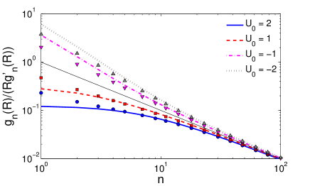
Figure S3: The ratio $g_{n}(R)/(Rg^{\prime}_{n}(R))$ vs the order $n$ of the radial function for several values of $U_{0}$ with $r_{0}=0.8$ and $R=1$. Comparison of the exact result in (SM4.2) (symbols) and the approximate expression in (S52) (lines). Thin solid line is the $1/n$ asymptotics (solution of the problem with $U_{0}\equiv 0$).

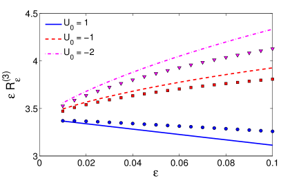
Figure S4: Infinite series ${\mathcal{R}}_{\varepsilon}^{(3)}$, multiplied by $\varepsilon$, as a function of the angular size $\varepsilon$ of the EW for $U_{0}=1$, $U_{0}=-1$ and $U_{0}=-2$ for $r_{0}=0$ and $R=1$. Symbols represent the exact result obtained by numerical summation of (19) involving the expression in (SM4.2), while curves show the asymptotic relation (IV) without the last infinite sum.

As a consequence, the leading asymptotic behaviour of $g_{n}(R)/(Rg^{\prime}_{n}(R))$ in (SM4.2) is entirely dominated by the first factor and hence, we have

$$\frac{g_{n}(R)}{Rg^{\prime}_{n}(R)}=\frac{1}{n}-\frac{\omega}{2n^{2}}+\frac{4\omega+\omega^{2}}{8n^{3}}+O\left(\frac{1}{n^{4}}\right)\,.$$ (S122)

The expansion in (S122) permits us to verify our general argument on the asymptotic behaviour of the ratio $g_{n}(R)/(Rg^{\prime}_{n}(R))$ in the limit $n\to\infty$, presented in the beginning of SM2 (see (S17)). Recalling that $\omega=RU^{\prime}(R)=U_{0}/(1-x_{0})$ and that for such a potential $U^{\prime\prime}(R)=0$, we observe a perfect coincidence of (S17), based on an intuitive (albeit quite plausible) argument, and the large-$n$ expansion of the inverse of the logarithmic derivative, evaluated for an exactly solvable case of a triangular-well potential $U(r)$. Further, we note that the large-$n$ behaviour of (S122) is dominated by the first factor, which is the solution for a particular case $r_{0}=0$. This implies, in turn, that in the large-$n$ limit the dependence on $r_{0}$ is fully embodied in the dimensionless parameter $\omega$.

Lastly, we compare the approximate expression (S52) for $g_{n}(R)/(Rg^{\prime}_{n}(R))$ and the exact result in (SM4.2) obtained for the triangular-well potential, see Fig. S3. We observe a fairly good agreement between the approximate formula (S52) and the exact result already for quite modest values of $n$, and notice that the agreement becomes even better for larger values of $R|U^{\prime}(R)|$. Accordingly, our approximate small-$\varepsilon$ expansion in (IV) (without the infinite sum in the last line) and the exact result for ${\mathcal{R}}_{\varepsilon}^{(3)}$ agree well with each other, see Fig. S4. The smaller $\varepsilon$, the better agreement is.

SM5 Triangular-well potential in 2D case

SM5.1 Solution of the inhomogeneous problem (22)

Integrating Eq. (22), we get

$$t_{0}(r)=\begin{cases}\displaystyle\frac{r_{0}^{2}-r^{2}}{4D}+H^{(2)}(\omega_{0})\qquad 0\leq r\leq r_{0},\cr H^{(2)}\left(\dfrac{\omega\,r}{R}\right)\hskip 42.67912ptr_{0}<r\leq R,\end{cases}$$ (S123)

where

$$H^{(2)}(z) =\frac{R^{2}}{D\omega^{2}}\biggl{[}\bigl{(}\omega_{0}^{2}/2+\omega_{0}+1\bigr{)}e^{-\omega_{0}}\int\limits_{z}^{\omega}dx~{}\frac{e^{x}}{x}-\omega(1-x_{0})+\ln x_{0}\biggr{]},$$ (S124)

Integrating (S123), one arrives at (IV.3). One also gets

$$t^{\prime}_{0}(R)=\frac{R}{D\omega^{2}}\biggl{(}\omega+1-\bigl{(}\omega_{0}^{2}/2+\omega_{0}+1\bigr{)}e^{\omega-\omega_{0}}\biggr{)}\,.$$ (S125)

SM5.2 Radial functions

In two dimensions, the solutions of (7) for a triangular-well potential read

$$\begin{split}u_{n}(z)&=z^{n}M(n,2n+1,z),\\ v_{n}(z)&=z^{-n}U(-n,-2n+1,z).\\ \end{split}$$ (S126)

Using the identities

$$\begin{split}zu^{\prime}_{n}(z)&=nz^{n}M(n+1,2n+1,z),\\ zv^{\prime}_{n}(z)&=-n^{2}z^{-n}U(-n+1,-2n+1,z),\\ \end{split}$$ (S127)

one gets

$$\begin{split}zu^{\prime}_{n}(z)-nu_{n}(z)&=\frac{nz^{n+1}}{2n+1}M(n+1,2n+2,z),\\ zv^{\prime}_{n}(z)-nv_{n}(z)&=-nz^{-n}U(-n,-2n,z),\\ \end{split}$$ (S128)

so that $w_{n}(z)$ becomes

$$w_{n}(z)=\frac{zu^{\prime}_{n}(z)-nu_{n}(z)}{zv^{\prime}_{n}(z)-nv_{n}(z)}=-\frac{M(n+1,2n+2,z)}{(2n+1)U(n+1,2n+2,z)}.$$ (S129)

Combining these equations we obtain the following explicit expression for the inverse logarithmic derivative of the radial functions in the 2D case with the triangular-well potential:

$$\frac{g_{n}(R)}{Rg^{\prime}_{n}(R)} =\frac{1}{n}~{}\frac{M(n,2n+1,\omega)}{M(n+1,2n+1,\omega)}\Bigg{(}1-\frac{U(n,2n+1,\omega)}{M(n,2n+1,\omega)}~{}w_{n}(\omega_{0})\Bigg{)}$$

$$\times\Bigg{(}1+\frac{nU(n+1,2n+1,\omega)}{M(n+1,2n+1,\omega)}~{}w_{n}(\omega_{0})\Bigg{)}^{-1}\,.$$ (S130)

As earlier in the 3D case, another representation can be obtained using (SM4.2)

$$\frac{g_{n}(R)}{Rg^{\prime}_{n}(R)}=\frac{1}{n}\,\frac{1-i_{n}(\omega)+(1+k_{n}(\omega))\,j_{n}(\omega,\omega_{0})}{1+i_{n}(\omega)+(1-k_{n}(\omega))\,j_{n}(\omega,\omega_{0})}\,,$$ (S131)

with

$$i_{n}(z) =\frac{I_{n+1/2}(z/2)}{I_{n-1/2}(z/2)}\,,\qquad k_{n}(z)=\frac{K_{n+1/2}(z/2)}{K_{n-1/2}(z/2)}\,,$$

$$j_{n}(z,z_{0}) =\frac{K_{n-1/2}(z/2)}{K_{n+1/2}(z_{0}/2)}\,\frac{I_{n+1/2}(z_{0}/2)}{I_{n-1/2}(z/2)}\,.$$ (S132)

As in the 3D case, we consider first the solution in the particular case when $r_{0}=0$. One may readily observe that here $w_{n}(0)=0$, which implies that (SM5.2) attains a simpler form

$$\frac{g_{n}(R)}{Rg^{\prime}_{n}(R)}=\frac{1}{n}~{}\frac{M(n,2n+1,\omega)}{M(n+1,2n+1,\omega)}\,,$$ (S133)

which is again just the first factor in (SM5.2).

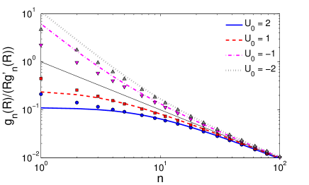
Figure S5: The ratio $g_{n}(R)/(Rg^{\prime}_{n}(R))$ vs the order $n$ of the radial function for several values of $U_{0}$, with $r_{0}=0.8$ and $R=1$. Comparison of the exact result in (SM5.2) (symbols) and the approximate expression in (S53) (lines). Thin solid line is the $1/n$ asymptotics (solution for $U_{0}\equiv 0$).

Turning to the limit $n\to\infty$, we find that the first factor in (SM5.2) obeys

$$\frac{1}{n}~{}\frac{M(n,2n+1,\omega)}{M(n+1,2n+1,\omega)}=\frac{1}{n}-\frac{\omega}{2n^{2}}+\frac{2\omega+\omega^{2}}{8n^{3}}+O\left(\frac{1}{n^{4}}\right)\,.$$ (S134)

Further, considering the second and the third factors on the right-hand-side of (SM5.2) we use a similar analysis as in the 3D case to find that their deviation from unity is exponentially small. This yields the following result for the behaviour of $g_{n}(R)/(Rg^{\prime}_{n}(R))$ in the limit $n\to\infty$:

$$\frac{g_{n}(R)}{Rg^{\prime}_{n}(R)} =\frac{1}{n}-\frac{\omega}{2n^{2}}+\frac{2\omega+\omega^{2}}{8n^{3}}+O\left(\frac{1}{n^{4}}\right)\,.$$ (S135)

Recalling the definition of $\omega$ and noting that for the triangular-well potential $U^{\prime\prime}(R)=0$, we again observe a perfect agreement between our expansion in (S19) and the exact result in (S135). We note as well that similarly to the 3D case, it appears that the large-$n$ behaviour is dominated by the solution with $r_{0}=0$, which implies that the dependence on this parameter of the interaction potential is fully taken into account by the parameter $\omega$.

Lastly, we compare the approximate expression (S53) for $g_{n}(R)/(Rg^{\prime}_{n}(R))$ and the exact result in (SM5.2) obtained for the triangular-well potential. We observe in Fig. S5 a fairly good agreement between the approximate formula (S53) and the exact result already for even smaller than in the 3D case values of $n$. The agreement becomes even better for larger values of $R|U^{\prime}(R)|$.

References

- (1) J. J. Lindemann and D. A. Lauffenburger, Biophys. J., 1985, 50, 295.
- (2) H-X. Zhou and R. Zwanzig, J. Chem. Phys., 1991, 94, 6147.
- (3) I. V. Grigoriev, Y. A. Makhnovskii, A. M. Berezhkovskii and V. Y. Zitserman, J. Chem. Phys., 2002, 116, 9574.
- (4) Y. Levin, M. A. Idiart and J. J. Arenzon, Physica A, 2005, 354, 95.
- (5) Z. Schuss, A. Singer and D. Holcman, Proc. Natl. Acad. Sci. USA, 2007, 104, 16098.
- (6) O. Bénichou and R. Voituriez, Phys. Rev. Lett., 2008, 100, 168105.
- (7) S. Pillay, M. Ward, A. Peirce and T. Kolokolnikov, Multiscale Model. Simul., 2010, 8, 803.
- (8) A. E. Lindsay, T. Kolokolnikov and J. C. Tzou, Phys. Rev. E, 2015, 91, 032111.
- (9) M. J. Byrne, M. N. Waxham and Y. Kubota, J. Comput. Neurosci., 2011, 31, 1.
- (10) A. M. Berezhkovskii and L. Dagdug, J. Chem. Phys., 2012, 136, 124110.
- (11) Z. Schuss, J. Sci. Comput., 2012, 53, 194.
- (12) P. C. Bressloff and J. M. Newby, Rev. Mod. Phys., 2013, 85, 135.
- (13) D. Holcman and Z. Schuss, J. Phys. A: Math. Theor., 2014, 47, 173001.
- (14) D. Holcman and Z. Schuss, SIAM Rev., 2014, 56, 213.
- (15) D. Holcman and Z. Schuss, Stochastic Narrow Escape in Molecular and Cellular Biology, Springer, New York, 2015.
- (16) M. J. Ward and J. B. Keller, SIAM J. Appl. Math., 1993, 53, 770.
- (17) G. Adam and M. Delbrück, Reduction of Dimensionality in Biological Diffusion Processes, in Structural Chemistry and Molecular Biology, edited by A. Rich and N. Davidson, Freeman, San Fransisco, 1968, pp. 198 - 215.
- (18) O. G. Berg, R. B. Winter and P. H. von Hippel, Biochemistry, 1981, 20, 6929.
- (19) O. Bénichou, M. Coppey, M. Moreau, P-H. Suet and R. Voituriez, Phys. Rev. Lett., 2005 94, 198101.
- (20) O. Bénichou, C. Loverdo, M. Moreau and R. Voituriez, Rev. Mod. Phys., 2011 83, 81.
- (21) G. Oshanin, H. S. Wio, K. Lindenberg and S. F. Burlatsky, J. Phys.: Condens. Matter, 2007, 19, 065142.
- (22) G. Oshanin, H. S. Wio, K. Lindenberg and S. F. Burlatsky, J. Phys. A.: Math. Theor., 2009, 42, 434008.
- (23) F. Rojo, J. Revelli, C. E. Budde, H. S. Wio, G. Oshanin and K. Lindenberg, J. Phys. A: Math. Theor., 2010, 43, 345001.
- (24) M. A. Lomholt, B. van den Broek, S.-M. J. Kalisch, G. J. L. Wuite and R. Metzler, Proc. Natl. Acad. Sci. USA, 2009, 106, 8204.
- (25) V. V. Palyulin, A. V. Chechkin and R. Metzler, J. Stat. Mech., 2014, P11031.
- (26) A. Godec and R. Metzler, Phys. Rev. E, 2015, 91, 052134.
- (27) G. Oshanin, M. Tamm and O. Vasilyev, J. Chem. Phys., 2010, 132, 235101.
- (28) O. Bénichou, D. Grebenkov, P. Levitz, C. Loverdo and R. Voituriez, Phys. Rev. Lett., 2010, 105, 150606.
- (29) O. Bénichou, D. Grebenkov, P. Levitz, C. Loverdo and R. Voituriez, J. Stat. Phys., 2011, 142, 657.
- (30) J. F. Rupprecht, O. Bénichou, D. Grebenkov and R. Voituriez, Phys. Rev. E, 2012, 86, 041135.
- (31) J. F. Rupprecht, O. Bénichou, D. Grebenkov and R. Voituriez, J. Stat. Phys., 2012, 147, 891.
- (32) F. Rojo and C. E. Budde, Phys. Rev. E, 2011, 84, 021117.
- (33) A. M. Berezhkovskii and A. V. Barzykin, J. Chem. Phys., 2012, 136, 054115.
- (34) F. Rojo, H. S. Wio and C. E. Budde, Phys. Rev. E, 2012, 86, 031105.
- (35) T. Calandre, O. Bénichou and R. Voituriez, Phys. Rev. Lett., 2014, 112, 230601.
- (36) A. M. Berezhkovsky and A. V. Barzykin, J. Chem. Phys., 2012, 136, 054115.
- (37) A. M. Berezhkovsky and L. Dagdug, J. Chem. Phys., 2012, 136, 124110.
- (38) J. Reingruber and D. Holcman, Phys. Rev. Lett., 2009, 103, 148102.
- (39) J. Reingruber and D. Holcman, J. Phys.: Condens. Matter, 2010, 22, 065103.
- (40) A. Godec and R. Metzler, First passage time statistics for two-channel diffusion, arXiv:1608.02397
- (41) O. Bénichou, M. Moreau and G. Oshanin, Phys. Rev. E, 2000, 61, 3388.
- (42) P. Malgaretti, I. Pagonabarraga and M. J. Rubi, Macromol. Symp., 2015, 357, 178.
- (43) P. Malgaretti, I. Pagonabarraga and M. J. Rubi, J. Chem. Phys., 2016, 144, 034901.
- (44) F. C. Collins and G. E. Kimball, J. Colloid. Sci., 1949, 4, 425.
- (45) D. Shoup, G. Lipari and A. Szabo, Biophys. J., 1981, 36, 697.
- (46) K. Solc and W. H. Stockmayer, J. Chem. Phys., 1971, 54, 2981; K. Solc and W. H. Stockmayer, Int. J. Chem. Kinet., 1973, 5, 733.
- (47) S. D. Traytak, Chem. Phys., 1997, 192, 1.
- (48) O. Bénichou and R. Voituriez, Phys. Rep., 2014, 539, 225.
- (49) V. M. Berdnikov and A. B. Doktorov, Chem. Phys., 1982, 69, 205.
- (50) G. Oshanin, M. N. Popescu and S. Dietrich, Active colloids in the context of chemical kinetics, arXiv:1607.05495
- (51) H. Sano and M. Tachiya, J. Chem. Phys., 1979, 71, 1276.
- (52) B. Sapoval, Phys. Rev. Lett., 1994, 73, 3314.
- (53) D. S. Grebenkov, in “Focus on Probability Theory”, Ed. L. R. Velle, Nova Science Publishers, 2006, pp. 135-169.
- (54) A. Singer, Z. Schuss, A. Osipov and D. Holcman, SIAM J. Appl. Math., 2008, 68, 844.
- (55) P. C. Bressloff, B. A. Earnshaw, and M. J. Ward, SIAM J. Appl. Math., 2008, 68, 1223.
- (56) D. S. Grebenkov, J. Chem. Phys., 2010, 132, 034104.
- (57) D. S. Grebenkov, Phys. Rev. E, 2010, 81, 021128.
- (58) C. W. Gardiner, Handbook of stochastic methods for physics, chemistry and the natural sciences, Springer: Berlin, 1985.
- (59) A. Singer, S. Schuss, D. Holcman, and R. S. Eisenberg, J. Stat. Phys., 2006, 122, 437.
- (60) A. Singer, S. Schuss, and D. Holcman, J. Stat. Phys., 2006, 122, 465.
- (61) C. Caginalp and X. Chen, Arch. Rational. Mech. Anal., 2012, 203, 329.
- (62) J.-F. Rupprecht, O. Bénichou, D. S. Grebenkov, and R. Voituriez, J. Stat. Phys., 2015, 158, 192.
- (63) D. S. Grebenkov, in First-Passage Phenomena and Their Applications, Eds. R. Metzler, G. Oshanin, S. Redner, World Scientific Press, 2014.