Gradient dynamics models for liquid films with soluble surfactant

Abstract

In this paper we propose equations of motion for the dynamics of liquid films of surfactant suspensions that consist of a general gradient dynamics framework based on an underlying energy functional. This extends the gradient dynamics approach to dissipative non-equilibrium thin film systems with several variables, and casts their dynamic equations into a form that reproduces Onsager’s reciprocity relations. We first discuss the general form of gradient dynamics models for an arbitrary number of fields and discuss simple well-known examples with one or two fields. Next, we develop the gradient dynamics (three field) model for a thin liquid film covered by soluble surfactant and discuss how it automatically results in consistent convective (driven by pressure gradients, Marangoni forces and Korteweg stresses), diffusive, adsorption/desorption, and evaporation fluxes. We then show that in the dilute limit, the model reduces to the well-known hydrodynamic form that includes Marangoni fluxes due to a linear equation of state. In this case the energy functional incorporates wetting energy, surface energy of the free interface (constant contribution plus an entropic term) and bulk mixing entropy. Subsequently, as an example, we show how various extensions of the energy functional result in consistent dynamical models that account for nonlinear equations of state, concentration-dependent wettability and surfactant and film bulk decomposition phase transitions. We conclude with a discussion of further possible extensions towards systems with micelles, surfactant adsorption at the solid substrate and bioactive behaviour.

I Introduction

Onsager’s evolution equations Onsa1931pr ; Onsa1931prb , based on the principle of detailed balance embedded in Onsager’s reciprocity relations, became a key tool for understanding the relaxational approach to equilibrium in a variety of physical processes. More recently, Doi Doi2011jpcm extended the range of this approach to processes in macroscopic soft matter systems, such as the swelling of gels and the dynamics of liquid crystals. It is less obvious that a similar approach can also be applied to processes out of equilibrium in spatially extended open systems. A well known example is the dynamics of single layer thin films in the long-wave (or lubrication) approximation OrDB1997rmp ; CrMa2009rmp where a single variable – the layer thickness – is sufficient for a description of the system. In this case, it is not a-priori obvious that an energy functional of thermodynamic origin exists for the system. Nevertheless, as noticed by Mitlin Mitl1993jcis for dewetting films and by Rosenau and Oron for thin films heated from below OrRo1992jpif , the dynamic equation for the layer thickness $h$ can be cast into a gradient dynamics form

$$\partial_{t}h\,=\,\nabla\cdot\left[Q^{\mathrm{c}}\nabla\frac{\delta\mathcal{F}}{\delta h}\right]-Q^{\mathrm{nc}}\left(\frac{\delta\mathcal{F}}{\delta h}-p_{\mathrm{vap}}\right),$$ (1)

showing that the evolution can be derived from a certain “energy” functional $\mathcal{F}[h]$. $p_{\mathrm{vap}}$ is the pressure of the vapour phase that may instead be incorporated into $\mathcal{F}$. Here and in the following $\partial_{t}$ denotes partial time derivatives and $\nabla$ is the two-dimensional (2D) spatial gradient operator. Eq. (1) is the general form in which the dynamics has both a conserved and a non-conserved contributions with mobilities $Q^{\mathrm{c}}(h)\geq 0$ and $Q^{\mathrm{nc}}(h)\geq 0$, respectively Thie2010jpcm .

The usual procedure of irreversible thermodynamics is thereby reversed: first comes a dynamic equation obtained through a series of simplifications, and then a suitable functional is assigned, ensuring a dissipative evolution toward a minimum of this energy. However, in the case of dewetting the energy functional is the “interface Hamiltonian” that is obtained via a systematic coarse-graining procedure from the microscale interaction energies BEIM2009rmp . Sometimes, even systems that are permanently out of equilibrium can be accommodated, as in the case of sliding droplets on an infinitely extended incline, where the correct thin film model can be brought into the form of a gradient dynamics with an underlying energy functional that includes potential energy EWGT2016arxiv .

Besides long-wave thin film equations, other examples of one-field gradient dynamics are the Cahn-Hilliard equation describing the demixing of a binary mixture, i.e., a purely conserved dynamics ($Q^{\mathrm{nc}}=0$) CaHi1958jcp ; Cahn1965jcp ; Lang1992 and the Allen-Cahn equation that models, for instance, the purely non-conserved dynamics ($Q^{\mathrm{c}}=0$) of the Ising model in the mean field continuum limit Lang1992 . In general, equations of the form (1) are ubiquitous. They appear with various choices of $\mathcal{F}$, not only in the context of the dynamics of films of non-volatile and volatile liquids on solid substrates OrDB1997rmp ; Mitl1993jcis ; PiPo2000pre ; Thie2014acis , but also as evolution equations for surface profiles in epitaxial growth SpVD1991prl ; GoDN1999pre ; GLSD2004prb ; Vved2004jpcm ; Thie2010jpcm , and, indeed, as models of one-component lipid bilayer adhesion dynamics GaCB1993jcis . Another field of application is in dynamical density functional theory (DDFT), describing the dynamics of the density distribution of colloidal particles MaTa1999jcp ; MaTa2000jpm ; ArEv2004jcp ; ArRa2004jpag .

Furthermore, many hydrodynamic two- and more-field long-wave models were developed that describe, e.g., the evolution of multilayer films, films of mixtures or surfactant-covered films CrMa2009rmp . Normally, they are not written in the gradient dynamics form. However, recently, the gradient dynamics approach was extended to several two-field models, namely, for the dewetting of two-layer films PBMT2004pre ; JHKP2013sjam , for the coupled decomposition and dewetting of a film of a binary mixture Thie2011epjst ; ThTL2013prl and for the evolution of a layer of insoluble surfactant on a thin liquid film ThAP2012pf . In all these cases, energies with a clear physical meaning can be given that may also be obtained via the coarse-graining procedures of statistical physics. Note though that the description of a thin two layer-film heated from below cannot be brought into the Onsager form PBMT2005jcp , marking the single layer case as a fortuitous ‘accident’. Nonetheless, certain out of equilibrium phenomena can be described via the addition of appropriate potential energies to the energy functional or, as in the case of dip coating and Langmuir–Blodgett transfer through “comoving frame terms” that account for a moving substrate that is withdrawn from a bath WTGK2015mmnp . Similar two-field gradient dynamics models exist for the dynamics of membranes SaGo2007pre ; HiKA2012pre or as DDFTs for mixtures ArRT2010pre ; archer2005jpcm .

The aim of this paper is to extend the gradient dynamics approach to describe the non-equilibrium dissipative dynamics of thin film systems with several variables, and to cast the dynamic equations into a form that reproduces Onsager’s reciprocity relations. A further aim is to incorporate interphase exchange processes, such as evaporation and surfactant dissolution to derive equations combining conserved (Cahn–Hilliard-type) and non-conserved (reaction-diffusion, or Allen–Cahn-type) terms. In doing so, several limitations of the known two-field models are alleviated. The particular example treated in detail is a thin liquid film that is covered by a soluble surfactant and rests on a solid substrate. The gradient dynamics model then describes the coupled evolution of the film height profile, the amount of surfactant within the film and the surface concentration dynamics (three field) model for the case of a thin liquid film covered by a soluble surfactant as sketched in Fig. 1.

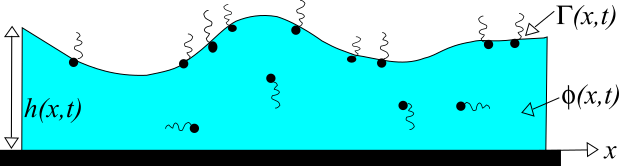
Figure 1: Sketch of the system under consideration. It consists of a film of liquid on a surface of thickness $h(x,t)$, that varies with location on the surface $x$ and with time $t$. On the liquid film free surface are surfactant molecules, with local density $\Gamma(x,t)$. The surfactant molecules have some solubility in the liquid and the local concentration within the body of the liquid is $\phi(x,t)$. We assume that $\phi$ does not vary vertically and only varies horizontally and with $t$. This is equivalent to treating $\phi$ as a height-averaged concentration. Over time there is exchange of surfactant molecules between the surface of the liquid and the bulk. There can also be condensation or evaporation of the liquid to vapour in the air above.

This paper is structured as follows: In the following section II we discuss the general form of gradient dynamics models, first, for an arbitrary number of fields in section II.1 and then in section II.2 we write the diffusion equation and the thin film equation as gradient dynamics and discuss known two-field models. Next, in section III we develop the gradient dynamics (three field) model for the case of a thin liquid film covered by a soluble surfactant and discuss in section IV special cases and extensions. We draw our conclusions in section V. Appendices A and B clarify an issue in the comparison of hydrodynamic long-wave approach and the present variational approach and give the variations of the energy functional in the most general case covered by the present work, respectively.

II General $N$-field model and known applications

II.1 General model

The dynamics of a spatially extended system may be characterised by the coupled evolution of $N$ scalar state variable fields (order parameter fields) $\mathbf{u}=(u_{1},u_{2},...,u_{n})^{\mathrm{T}}$. Not too far from equilibrium, the dynamics is governed by a single equilibrium free energy functional $\mathcal{F}[\mathbf{u}]$, i.e., it is a gradient dynamics. Using Einstein’s index notation that presumes summation over repeated indices, the coupled evolution equations read

$$\partial_{t}u_{a}=\nabla_{\alpha}\left[Q^{\mathrm{c}}_{ab}\nabla_{\alpha}\frac{\delta\mathcal{F}}{\delta u_{b}}\right]-Q^{\mathrm{nc}}_{ab}\frac{\delta\mathcal{F}}{\delta u_{b}}$$ (2)

where $\alpha=1,2,\dots,d$ refers to spatial coordinates and $a,b=1,\dots,n$ refer to the different order parameter fields that might have a conserved, or non-conserved, or mixed dynamics. Here, $Q^{\mathrm{c}}_{ab}(\mathbf{u})$ and $Q^{\mathrm{nc}}_{ab}(\mathbf{u})$ represent $n\times n$ dimensional positive definite and symmetric mobility matrices for the conserved and non-conserved parts of the dynamics, respectively. The mobilities $Q^{\mathrm{c}}_{ab}$ govern the fluxes $j_{a}=-Q^{\mathrm{c}}_{ab}\nabla({\delta\mathcal{F}}/{\delta u_{b}})$ of the conserved part of the dynamics for all order parameters $u_{a}$. These are given as linear combinations of the influences of all thermodynamic forces $-\nabla({\delta\mathcal{F}}/{\delta u_{b}})$, i.e. are linear in the thermodynamic forces. In contrast, the coefficients $Q^{\mathrm{nc}}_{ab}$ give the transition rates between fields and are also linear combinations of the thermodynamic potentials ${\delta\mathcal{F}}/{\delta u_{a}}$.

It is straightforward to show that the free energy $\mathcal{F}[u_{1},\dots,u_{n}]$ is a Lyapunov functional, i.e., it monotonically decreases in time:

$$\frac{\mathrm{d}}{\mathrm{d}t}\mathcal{F}[u_{1},\dots,u_{n}] =\int\limits_{\Omega}\frac{\delta\mathcal{F}}{\delta u_{a}}\frac{\partial u_{a}}{\partial t}~{}\mathrm{d}^{d}x$$

$$=\int\limits_{\Omega}\frac{\delta\mathcal{F}}{\delta u_{a}}\nabla_{\alpha}\left[Q^{\mathrm{c}}_{ab}\nabla_{\alpha}\frac{\delta\mathcal{F}}{\delta u_{b}}\right]~{}\mathrm{d}^{d}x-\int\limits_{\Omega}\frac{\delta\mathcal{F}}{\delta u_{a}}Q^{\mathrm{nc}}_{ab}\frac{\delta\mathcal{F}}{\delta u_{b}}~{}\mathrm{d}^{d}x$$

$$=-\int\limits_{\Omega}\left(\nabla_{\alpha}\frac{\delta\mathcal{F}}{\delta u_{a}}\right)Q^{\mathrm{c}}_{ab}\left(\nabla_{\alpha}\frac{\delta\mathcal{F}}{\delta u_{b}}\right)~{}\mathrm{d}^{d}x-\int\limits_{\Omega}\frac{\delta\mathcal{F}}{\delta u_{a}}Q^{\mathrm{nc}}_{ab}\frac{\delta\mathcal{F}}{\delta u_{b}}~{}\mathrm{d}^{d}x\leq 0.$$ (3)

where $\Omega$ is the domain in which the system is defined. Above we used Eq. (2) and partial integration, assuming periodic or no-flux boundary conditions.

A further advantage of the general formulation is the ease with which one may change the choice of variables $u_{a}$. If new order parameter fields $\tilde{u}_{a}$ are introduced via a linear transformation $\tilde{u}_{a}=R_{ab}u_{b}$ the kinetic equations for the new fields are

$$\partial_{t}\tilde{u}_{a}=\nabla_{\alpha}\left[\widetilde{Q}^{\mathrm{c}}_{ab}(\tilde{u}_{1},\dots,\tilde{u}_{n})\nabla_{\alpha}\frac{\delta\mathcal{F}}{\delta\tilde{u}_{b}}\right]\,-\,\widetilde{Q}^{\mathrm{nc}}_{ab}(\tilde{u}_{1},\dots,\tilde{u}_{n})\frac{\delta\mathcal{F}}{\delta\tilde{u}_{b}}$$ (4)

with $\widetilde{Q}^{\mathrm{i}}_{ab}=R_{ad}Q^{\mathrm{i}}_{de}R_{be}$ ($\mathrm{i}=\mathrm{c},\mathrm{nc}$) where we take into account that $\delta\mathcal{F}/\delta u_{a}=R_{ba}\delta\mathcal{F}/\delta\tilde{u}_{b}$. For two conserved fields, similar relations were already given in Refs. XuTQ2015jpcm ; WTGK2015mmnp .

Up to here, we have not specified the free energy $\mathcal{F}[u_{1},\dots,u_{n}]$ that can, in principle, be an arbitrary functional of the order parameter fields. If $\mathcal{F}$ is a multiple integral, Eq. (2) becomes a system of integro-differential equations, as is often the case in DDFT for colloids ArEv2004jcp . However, often the kernel is expanded in derivatives of the order parameter fields and Eq. (2) corresponds to a system of partial differential equations. Examples are Phase Field Crystal (PFC) models ELWG2012ap and membrane models HiKA2009c ; HiKA2012pre where the highest order terms in the energy are $\sim(\Delta u)^{2}$. Here we restrict our attention to a lower order and only consider models where the highest order terms are $\sim(\nabla u)^{2}$. Then the general form is

$$\mathcal{F}[u_{1},\dots,u_{n}]=\int\limits_{\Omega}\left[\frac{1}{2}(\nabla_{\alpha}u_{a})~{}\Sigma_{ab}~{}(\nabla_{\alpha}u_{b})+f(u_{1},\dots,u_{n})\right]~{}\mathrm{d}^{d}x,$$ (5)

where we have introduced in the free energy a symmetric $n\times n$ dimensional gradient interaction matrix $\Sigma_{ab}$ that, in principle, may itself also depend on $\mathbf{u}$. The integrand may also contain metric factors (see below).

Before we come in Section III to the case of liquid films that are covered with a soluble surfactant, we briefly review in Section II.2 some basic examples where only one or two order parameter fields are involved.

II.2 Specific known examples of gradient dynamics

II.2.1 Diffusion equation

In the dilute limit, the diffusion of a species with part-per-volume concentration $c$ in a quiescent carrier medium can be represented as the conserved gradient dynamics

$$\partial_{t}c\,=\,\nabla\cdot\left[Q^{\mathrm{c}}_{cc}\nabla\frac{\delta\mathcal{F}}{\delta c}\right],$$ (6)

with the purely entropic Helmholtz free energy functional

$$\mathcal{F}[c]\,=\,\frac{kT}{l^{3}}\int c[\ln c-1]\,dV,$$ (7)

where $k$ is Boltzmann’s constant, $T$ is the temperature and $l$ is a molecular length scale. The mobility function in Eq. (6) is $Q^{\mathrm{c}}_{cc}=\widetilde{D}c$ and can be obtained via Onsager’s variational principle Doi2011jpcm ; Doi2013 ; XuTQ2015jpcm . Here, $\widetilde{D}$ is the molecular mobility. This corresponds to $\partial_{t}c\,=\,-\nabla\cdot j_{\mathrm{diff}}$ where Fick’s law takes the form $j_{\mathrm{diff}}=-\widetilde{D}c\nabla\mu=-D\nabla c$ with the chemical potential $\mu=\delta\mathcal{F}/\delta c=(kT/l^{3})\ln c$, i.e. $D=\widetilde{D}c\,d\mu/dc=\widetilde{D}kT/l^{3}$.

The equivalence of Eq. (6) and the standard diffusion equation has been easily shown, and now allows one to use the advantages of the gradient dynamics form, namely, the straightforward way to account for free energies that are not purely entropic. If, for instance, one replaces the integrand in $\mathcal{F}[c]$ of Eq. (7) by the sum of a double-well potential and a squared gradient term, one obtains the Cahn-Hilliard equation (then using a constant $Q^{\mathrm{c}}_{cc}$) Cahn1965jcp .

II.2.2 Thin films of simple liquids

As discussed above, Eq. (1) describes the evolution of the height profile of a thin liquid film on a solid substrate for non-volatile ($Q^{\mathrm{nc}}(h)=0$) or volatile ($Q^{\mathrm{nc}}(h)\geq 0$) liquids. Detailed discussions of the various physical situations treated can be found in OrDB1997rmp ; Thie2010jpcm ; Thie2014acis . In the most basic case of mesoscopic hydrodynamics, only the influence of capillarity and wettability is considered. The corresponding free energy $\mathcal{F}[h]$ is then

$$\mathcal{F}[h]\,=\,\int\left[\frac{\gamma}{2}(\nabla h)^{2}+g(h)\right]d^{2}x,$$ (8)

where $\gamma$ is the surface tension of the liquid and $g(h)$ is a local free energy (wetting or adhesion energy, or binding potential), related to the Derjaguin (or disjoining) pressure $\Pi(h)$ by $\Pi=-dg(h)/dh$ Genn1985rmp . Note, that varying sign conventions are used throughout the literature. For particular forms of $\Pi$, see, e.g., Refs. Genn1985rmp ; Israelachvili2011 ; Mitl1993jcis ; OrDB1997rmp ; PiPo2000pre ; KalliadasisThiele2007 . Similar expressions are obtained as “interface Hamiltonians” in the context of wetting transitions BEIM2009rmp . Therefore mesoscopic thin film (or two-dimensional) hydrodynamics might be considered as a gradient dynamics on the underlying interface Hamiltonian. Note that recently such mesoscopic wetting energies have been extracted via parameter passing methods from different microscopic models (molecular dynamics and density functional theory) TMTT2013jcp ; HuTA2015jcp . Without slip at the substrate, $Q^{\mathrm{c}}\equiv Q^{\mathrm{c}}_{hh}=h^{3}/3\eta$, where $\eta$ is the dynamic viscosity. Different slip models can be accommodated by alternative choices of $Q^{\mathrm{c}}_{hh}$ MWW2005jem . Although several functions $Q^{\mathrm{nc}}(h)$ are discussed in the literature for the case of volatile liquids (see, e.g., Thie2014acis ), often a constant is used LyGP2002pre ).

II.2.3 Two-field models

In the context of thin film hydrodynamics, two-field gradient dynamics models were presented and analysed (i) for dewetting two-layer films on solid substrates, i.e., staggered layers of two immiscible fluids PBMT2004pre ; PBMT2005jcp ; JHKP2013sjam , (ii) for decomposing and dewetting films of a binary liquid mixture (with non-surface active components) Thie2011epjst ; ThTL2013prl , and (iii) for the dynamics of a liquid film that is covered by an insoluble surfactant ThAP2012pf . In all three cases, the model has the form (2) with $a,b=1,2$ and all $Q^{\mathrm{nc}}_{ab}=0$ (purely conserved dynamics). The conserved fields $u_{1}$ and $u_{2}$ represent in case (i) the lower layer thickness $h_{1}$ and overall thickness $h_{2}$, respectively PBMT2004pre ; PBMT2005jcp ; JHKP2013sjam or the lower and upper layer thickness BCJP2013epje (the transformation between the two formulations follows from the discussion around Eq. (4)). In case (ii), $u_{1}$ and $u_{2}$ represent the film height $h$ and the effective solute height $\psi=ch$, respectively, where $c$ is the height averaged concentration. Finally, in case (iii), $u_{1}$ and $u_{2}$ represent the film height $h$ and the surfactant coverage $\widetilde{\Gamma}$ (that is projected on the cartesian substrate plane), respectively ThAP2012pf .

As already emphasised, a crucial point in cases (ii) and (iii) is the choice of the two fields that can be varied independently of each other. This is not the case if, e.g., film height $h$ and height averaged concentration $c$ are used in case (ii), since then a variation in the height for fixed particle number per substrate area implies that $c$ varies Thie2011epjst . In case (iii), the projected coverage $\widetilde{\Gamma}$ has to be used since the surfactant coverage $\Gamma$ on the free surface and the height profile $h$ are not independent ThAP2012pf : If the slope of $h$ changes locally, the surface area changes and so also $\Gamma$. Therefore, for a fixed local number of surfactant molecules, the local concentration changes without any surfactant transport. If one uses dependent fields, one is not able to employ the general form (2). Note that in Refs. Clar2005m ; TCPM2010sm case (ii) has been treated employing a gradient dynamics for $h$ and $c$. For a further comparison with the approach employed in Thie2011epjst ; ThTL2013prl , see Ref. Thie2014acis . In all three cases (i) to (iii) the underlying free energy functionals have a clear thermodynamic significance. They may be seen as extensions of the interface Hamiltonian for a single adsorbed layer, and the individual terms may be obtained from equilibrium statistical physics. As expected, the mobility matrices $\mathbf{Q}^{\mathrm{c}}$ are positive definite and symmetric PBMT2004pre ; BCJP2013epje ; ThTL2013prl ; ThAP2012pf . All their entries are low order polynomials in the respective fields $u_{1}$ and $u_{2}$. In particular, in cases (ii) and (iii), one has

$$\mathbf{Q}^{\mathrm{c}}\,=\,\,=\,\frac{1}{3\eta}\left(\begin{array}[]{cc}u_{1}^{3}&qu_{1}^{2}u_{2}\\[1.29167pt] qu_{1}^{2}u_{2}&\quad ru_{1}u_{2}^{2}+3\widetilde{D}\eta u_{2}\end{array}\right).$$ (9)

where $\widetilde{D}$ is a respective molecular mobility related to diffusion, and $q=r=1$ in case (ii) and $q=3/2$, $r=3$ in case (iii). Actually, in the parametrisation of Ref. JHKP2013sjam , the mobility matrix $\mathbf{Q}^{\mathrm{c}}$ of case (i) also agrees with case (iii) if the diffusion term $3\widetilde{D}\eta u_{2}$ is replaced by $\eta_{\mathrm{r}}u_{2}^{3}$ where $\eta_{\mathrm{r}}$ is the viscosity ratio of the two layers.

Note in particular that cases (ii) and (iii) in the respective low concentration limit give the known hydrodynamic thin film equations coupled to the equation for the solute / surfactant as discussed in detail in Refs. Thie2011epjst and ThAP2012pf , respectively. It recovers also a number of other special cases and can be employed to devise models that incorporate various energetic cross-couplings in a thermodynamically consistent manner. Examples include wetting energies that depend on solute or surfactant concentration, effects of surface rigidity for surfactant covered films, free energies of mixing/decomposition including gradient contributions, etc. It also allows one to discuss the influence of solutes / surfactants on evaporation.

Note that the discussion above mixes the possible extensions in cases (ii) and (iii) that are separately discussed in Thie2011epjst and ThAP2012pf , respectively. It was noted in ThTL2013prl that the two-field model for a film of a mixture cannot accommodate a solutal Marangoni effect by simply incorporating a concentration-dependent surface tension since this breaks the gradient dynamics structure. Another disadvantage of the two-field model is that most surfactants are soluble, a situation that cannot be treated via case (iii). In the following, we develop a three-field model that alleviates all the mentioned problems.

III Soluble surfactant - gradient dynamics model

III.1 Energy functional

We consider a thin film of liquid of thickness $h$ on a solid substrate with a free surface that is covered by a soluble surfactant, i.e., part of the surfactant is dissolved in the bulk of the film and part is adsorbed at the free surface – see Fig. 1. We neglect adsorption at the solid-liquid interface and micelle formation but discuss in teh conclusion how they can be incorporated. The surfactant concentration $\phi$ within the film represents a height-averaged concentration, i.e., it is assumed that the concentration is nearly uniform over the film layer thickness. The system is considered in relaxational situations, i.e., the boundary conditions do not sustain energy or mass fluxes. Therefore, we expect the system dynamics to follow a pathway that approaches a static equilibrium. In the absence of evaporation and surfactant exchange between the interface and the bulk solution, the approach to equilibrium can be described by gradient dynamics for three independent fields: the film thickness $h(\mathbf{r},t)$, the local amount of dissolved surfactant $\psi(\mathbf{r},t)=h(\mathbf{r},t)\,\phi(\mathbf{r},t)$, and the surfactant concentration at the interface projected onto a cartesian reference plane $\widetilde{\Gamma}(\mathbf{r},t)$. The surfactant concentration on the interface is given by $\Gamma=\widetilde{\Gamma}/\sqrt{a}$ where $a$ is the determinant of the surface metric tensor (see below). Here $\mathbf{r}=(x,y)$ are “horizontal” coordinates in the substrate plane. The fields $\phi$ and $\Gamma$ are expressed as volume fraction and area fraction concentrations, respectively, i.e., they are both dimensionless. As emphasised in section II.2.3 for the two-field cases, variations in $h$, $\phi$ and $\Gamma$ are not independent, whilst variations with respect to $h$, $\psi$ and $\widetilde{\Gamma}$ are independent.

The general expression for the energy includes surface and bulk contributions:

$$\mathcal{F} = \mathcal{F}_{\mathrm{s}}+\mathcal{F}_{\mathrm{b}}=\int(\mathcal{L}_{\mathrm{s}}+\mathcal{L}_{\mathrm{b}})dxdy,$$ (10)

$$\mathcal{L}_{\mathrm{s}} = \left[\frac{\kappa_{\mathrm{s}}}{2}a^{\alpha\beta}(\partial_{\alpha}\Gamma)(\partial_{\beta}\Gamma)+f_{\mathrm{s}}(\Gamma)\right]\sqrt{a}+g(h),$$ (11)

$$\mathcal{L}_{\mathrm{b}} = h\left[\frac{\kappa}{2}|\nabla\phi|^{2}+f(\phi)\right].$$ (12)

The interfacial terms in Eq. (11) depend on the surface metric tensor $a_{\alpha\beta}=\delta_{\alpha\beta}+\partial_{\alpha}h\partial_{\beta}h$ [where we exclude overhangs in order to use a Monge representation $h(x,y)$] and its inverse $a^{\alpha\beta}$; $a$ is the determinant of $a_{\alpha\beta}$ and determines the extension of the interface, and $\delta_{\alpha\beta}$ is the Cartesian metric of the planar substrate or a planar surface $h=$ const. Distinction between lower (covariant) and upper (contravariant) indices is essential for a non-Euclidean surface metric. The wetting potential $g(h)$ in Eq. (11) describes the interactions with the substrate that determine the Derjaguin (or disjoining) pressure $\Pi(h)=-dg(h)/dh$ (cf. Section II.2.2). The first terms in parentheses in Eqs. (11) and (12) contain the interfacial and bulk rigidity coefficients $\kappa_{\mathrm{s}}$ and $\kappa$, respectively, and penalize surfactant concentration gradients. The second terms in the parentheses in each case takes account of molecular interactions. $f_{\mathrm{s}}(\Gamma)$ contains the free energy contribution due to the presence of surfactant molecules at the interface. In the limit $\Gamma\to 0$, then this is just the pure liquid-vapour surface tension, i.e. $f_{\mathrm{s}}(\Gamma\to 0)=\gamma_{0}$, but more generally

$$f_{\mathrm{s}}(\Gamma)=\gamma_{0}+\frac{kT}{l_{s}^{2}}\Gamma[\ln\Gamma-1]+f_{s}^{ex}(\Gamma).$$ (13)

The second term is the contribution to the free energy when the amount of surfactant on the surface is low enough that interactions between molecules are negligible and can be treated as a 2D ideal-gas. $l_{s}$ is a molecular length scale related to the size of the adsorbed surfactant molecules ($l_{s}^{2}$ is the area on the surface occupied by a surfactant molecule). As the surface coverage $\Gamma$ increases, then the excess free energy $f_{\mathrm{s}}^{ex}(\Gamma)$ gives an increasing contribution. For example, treating the surfactant on the surface via a lattice-gas approximation, one would write

$$f_{\mathrm{s}}^{ex}(\Gamma)=\frac{kT}{l_{s}^{2}}[\Gamma+(1-\Gamma)\ln(1-\Gamma)]-\frac{b}{2}\Gamma^{2}$$ (14)

where the first (entropic) excluded volume term comes from assuming only one surfactant molecule can occupy a site of area $l_{\mathrm{s}}^{2}$ on the surface and the final term is a simple mean-field term coming from the attraction between pairs of neighbouring surfactant molecules. If the attraction strength parameter $b>0$ is sufficiently large, then surface phase transitions may occur. An alternative approximation might be $f_{\mathrm{s}}^{ex}(\Gamma)=f_{hd}(\Gamma)-b\Gamma^{2}/2$, where $f_{hd}$ is the hard-disk excess free energy – see for example the approximations in Refs. APER2007jcp ; AIPR2008jpm .

Similarly, the bulk free energy in Eq. (12) can be written as:

$$f(\phi)=\frac{kT}{l^{2}}\phi[\ln\phi-1]+f_{b}^{ex}(\phi),$$ (15)

where $l$ is a molecular length scale related to the surfactant molecules in solution ($l^{3}$ is the volume occupied by a surfactant molecule). The simplest approximation is to assume $l_{s}=l$. $f_{b}^{ex}(\phi)$ is the bulk excess contribution which in general may be written as a virial expansion $f_{b}^{ex}(\phi)=\sum_{i=2}^{\infty}c_{i}\phi^{i}$, with coefficients $c_{i}$ that depend on the temperature. Alternatively one may approximate, e.g. by assuming a lattice-gas free energy

$$f_{b}^{ex}=\frac{kT}{l^{2}}[\phi+(1-\phi)\ln(1-\phi)]-\frac{b_{b}}{2}\phi^{2},$$ (16)

where $b_{b}>0$ is an inter-surfactant molecule attraction strength parameter. Or, instead one could assume $f_{b}^{ex}(\phi)=f_{cs}(\phi)-b_{b}\phi^{2}/2$, where $f_{cs}(\phi)$ is the Carnahan-Starling approximation for the hard-sphere excess free energy HansenMcDonald2006 . Specific cases for the excess contributions $f_{\mathrm{s}}^{ex}(\Gamma)$ and $f_{\mathrm{ex}}(\phi)$ will be discussed below in Section III.5.2.

III.2 Pressures, chemical potentials and surface stress

The expression for pressure $p=\delta\mathcal{F}/\delta h$ is obtained by calculating the variation of Eq. (10) with respect to $h$ for fixed $\widetilde{\Gamma},\psi$. The variation of $\mathcal{F}_{\mathrm{s}}$ depends on the surface metric and uses the relations

$$\delta a=a\,a^{\alpha\beta}\delta a_{\alpha\beta}=-a\,a_{\alpha\beta}\delta a^{\alpha\beta},\quad g\delta a_{\alpha\beta}=g\delta(\partial_{\alpha}h\partial_{\beta}h)=-[\partial_{\alpha}(g\partial_{\beta}h)+\partial_{\beta}(g\partial_{\alpha}h)]\delta h,$$ (17)

where $g$ is an arbitrary function of the surface coordinates. Also note that $a^{\alpha\beta}a_{\alpha\beta}=\delta_{\alpha}^{\alpha}=2$. As mentioned above, $\Gamma$ changes with surface extension or contraction, so that before the variation of $\mathcal{F}_{\mathrm{s}}$ is computed one needs to replace $\Gamma=\widetilde{\Gamma}/\sqrt{a}$, where $\widetilde{\Gamma}$ is a reference surfactant coverage of a planar interface, or coverage per substrate area ThAP2012pf . Similarly, one must replace $\phi\to\psi/h$ before the variation of $\mathcal{F}_{\mathrm{b}}$ is computed Thie2011epjst . This yields

$$p = \frac{\delta\mathcal{F}}{\delta h}=-\partial_{\alpha}\left(\sqrt{a}\,\sigma^{\alpha\beta}\partial_{\beta}h\right)-\Pi(h)+p_{\mathrm{b}},$$ (18)

$$p_{\mathrm{b}} = \frac{\delta\mathcal{F}_{\mathrm{b}}}{\delta h}=p_{\mathrm{osm}}{+}\kappa\left[\frac{1}{2}|\nabla\phi|^{2}+\frac{\phi}{h}\nabla\cdot(h\nabla\phi)\right],\quad p_{\mathrm{osm}}=f(\phi)-\phi f^{\prime}(\phi).$$ (19)

where $p_{\mathrm{osm}}$ is the bulk osmotic pressure. With solely the ideal-gas (entropic) terms in Eq. (15), it becomes $p_{\mathrm{osm}}=-kT\phi/l^{3}$. Note too that $\nabla$ is the 2D gradient operator, and $\nabla^{2}$ is the 2D Laplacian. The second term in Eq. (18) is the disjoining pressure, while the first term contains the interfacial stress

$$\sigma^{\alpha\beta} = \frac{\delta\mathcal{F}_{\mathrm{s}}}{\delta a_{\alpha\beta}}=\frac{1}{2}a^{\alpha\beta}[f_{\mathrm{s}}(\Gamma)-\Gamma f_{\mathrm{s}}^{\prime}(\Gamma)]-\frac{\kappa_{\mathrm{s}}}{4}a^{\alpha\beta}a^{\gamma\delta}\partial_{\gamma}\Gamma\partial_{\delta}\Gamma$$ (20)

$$+ \frac{\kappa_{\mathrm{s}}\Gamma}{4}a^{\alpha\beta}\left[\partial_{\gamma}\left(\sqrt{a}\,a^{\gamma\delta}\partial_{\delta}\Gamma\right)+\partial_{\delta}\left(\sqrt{a}\,a^{\gamma\delta}\partial_{\gamma}\Gamma\right)\right].$$

In particular, the standard surface tension is defined as

$$\gamma(\Gamma)=a_{\alpha\beta}(\sigma^{\alpha\beta})_{\kappa_{\mathrm{s}}\to 0}=f_{\mathrm{s}}(\Gamma)-\Gamma f_{\mathrm{s}}^{\prime}(\Gamma).$$ (21)

The function $f_{\mathrm{s}}$ in Eq. (13) with Eq. (14) for $b=0$ results then in what is sometimes called the Langmuir equation of state PaSt1996pf ; KrVM2004pf or the Von Szyckowski equation EgPS1999jfm

$$\gamma=\gamma_{0}+\frac{kT}{l_{\mathrm{s}}^{2}}\ln(1-\Gamma),$$ (22)

i.e., for $\Gamma\ll 1$ one has $\gamma\approx\gamma_{0}-kT\Gamma/l_{\mathrm{s}}^{2}=\gamma_{0}-\gamma_{\Gamma}\Gamma$, where we introduced the Marangoni coefficient $\gamma_{\Gamma}=kT/l_{\mathrm{s}}^{2}$ for the resulting linear solutal Marangoni effect. Note that with $b\neq 0$ in Eq. (14) one obtains the Frumkin equation of state as given in PaSt1996pf and further discussed below in section III.5.2.

The surface chemical potential $\mu_{\mathrm{s}}$ is obtained by varying Eq. (10) with respect to $\widetilde{\Gamma}$:

$$\mu_{\mathrm{s}}=\frac{\delta\mathcal{F}}{\delta\widetilde{\Gamma}}=\frac{df_{\mathrm{s}}}{d\Gamma}-\frac{\kappa_{\mathrm{s}}}{2}\left[\partial_{\alpha}\left(a^{\alpha\beta}\partial_{\beta}\Gamma\right)+\partial_{\beta}\left(a^{\alpha\beta}\partial_{\alpha}\Gamma\right)\right].$$ (23)

Finally, the bulk chemical potential is ThAP2016note1

$$\mu=\frac{\delta\mathcal{F}}{\delta\psi}=f^{\prime}(\phi)-\kappa h^{-1}\nabla\cdot\left(h\nabla\phi\right).$$ (24)

The mechanical interaction between the surfactant layer and the bulk liquid is carried by the balance of the interfacial stress and the viscous stress in the bulk fluid proportional to the normal derivative of the velocity $v^{\alpha}$ tangential to the interface and the bulk viscosity $\eta$:

$$\sigma^{\alpha\beta}{}_{;\beta}=\eta v^{\alpha}{}_{;n},$$ (25)

where the semicolon denotes the covariant derivative necessary when vectors defined on a curved interface are involved. This equation reduces to the commonly used tangential stress balance including the Marangoni force when the rigidity $\kappa_{\mathrm{s}}$ is neglected.

III.3 Thin film hydrodynamics

The above general expressions for the surface stress and pressure can be simplified in the case when the curvature and inclination are small so that the long-wave or lubrication approximation can be made. To this end, we scale $\partial_{\alpha}\sim O(\epsilon)$, $v^{\alpha}\sim O(\epsilon)$, $\partial_{t}\sim O(\epsilon^{2})$ and retain terms up to the lowest relevant order in $\epsilon\ll 1$. With this scaling, $a_{\alpha\beta}$ differs from the Cartesian surface metric $\delta_{\alpha\beta}$ by $O(\epsilon^{2})$, so that $a_{\alpha\beta}=\delta_{\alpha\beta}+\epsilon^{2}\partial_{\alpha}h\partial_{\beta}h$ and its inverse is, to leading order, $a^{\alpha\beta}=\delta_{\alpha\beta}-\epsilon^{2}\partial_{\alpha}h\partial_{\beta}h$. Then, the above expressions can be rewritten using Cartesian coordinates $x_{\alpha}$ spanning the plane of the substrate, whereby the distinction between covariant and contravariant tensors disappears (so that all indices can be written as subscripts) and covariant derivatives are replaced by usual partial derivatives. Retaining the leading order terms only, Eqs. (18) – (23) become

$$p=\frac{\delta\mathcal{F}}{\delta h}=-\nabla\cdot\left[(\gamma_{0}-p_{\mathrm{s}})\nabla h\right]-\Pi(h)+p_{\mathrm{b}},$$ (26)

$$p_{\mathrm{s}}=\gamma_{0}-\gamma(\Gamma)-\kappa_{\mathrm{s}}\left(\Gamma\nabla^{2}\Gamma-\frac{1}{2}|\nabla\Gamma|^{2}\right)$$ (27)

$$\mu_{\mathrm{s}}=\frac{\delta\mathcal{F}}{\delta\widetilde{\Gamma}}=f_{\mathrm{s}}^{\prime}(\Gamma)-\kappa_{\mathrm{s}}\nabla^{2}\Gamma,$$ (28)

where we have used $\sigma_{\alpha\beta}=\delta_{\alpha\beta}\,(\gamma_{0}-p_{\mathrm{s}})$ and where $p_{\mathrm{s}}$ is the surface pressure that captures the difference between reference surface tension without surfactant $\gamma_{0}$ and the full concentration-dependent expression (including rigidity). Further, $p_{\mathrm{b}}$ and $p_{\mathrm{osm}}$ remain as in Eq. (19) while $\mu$ is still given by Eq. (24).

The bulk flow field is computed by solving the modified Stokes equation, also called the momentum equation of model-H JaVi1996pf ; ThMF2007pf . Its relevant components are parallel to the substrate plane:

$$\eta\mathbf{v}^{\prime\prime}(z)=\nabla{p}+\phi\nabla\mu.$$ (29)

where $\mathbf{v}$ is the 2D vector of the velocities parallel to the substrate plane. An alternative form of equation (29) can be obtained using the relation

$$\nabla p_{\mathrm{b}}=f^{\prime\prime}(\phi)\nabla\phi-\kappa\nabla\left[\frac{1}{2}|\nabla\phi|^{2}+\frac{\phi}{h}\nabla\cdot(h\nabla\phi)\right]=-\phi\nabla{\mu}+\frac{\kappa}{h}\nabla(h|\nabla\phi|^{2}),$$ (30)

which reduces the right-hand side of the Stokes equation (29) to

$$\nabla(p-p_{\mathrm{b}})+\nabla p_{\mathrm{b}}+\phi\nabla\mu=\nabla\widehat{p}+\frac{\kappa}{h}\nabla(h|\nabla\phi|^{2}),$$ (31)

where $\widehat{p}$ is the effective pressure excluding $p_{\mathrm{b}}$. This shows that osmotic pressure $p_{\mathrm{osm}}$ does not affect hydrodynamic flow (as $\nabla p_{\mathrm{osm}}=-\phi\nabla\mu$), while the contribution of the bulk rigidity is expressed by the last term in the above relation.

Solving Eq. (29) in the lubrication approximation with the no-slip boundary condition at the substrate plane $z=0$ and the momentum balance condition (25) at the interface $z=h$ yields

$$\mathbf{v}=-\frac{z}{\eta}\left[\nabla p_{\mathrm{s}}+\left(h-\frac{z}{2}\right)(\nabla{p}+\phi\nabla\mu)\right].$$ (32)

Integrated over the local film thickness, this leads to the convective fluid flux

$$\mathbf{J}_{\mathrm{conv}}=\int_{0}^{h}\mathbf{v}dz=-\frac{h^{2}}{2\eta}\nabla p_{\mathrm{s}}-\frac{h^{3}}{3\eta}(\nabla{p}+\phi\nabla\mu),$$ (33)

and the interfacial velocity $\mathbf{v}_{\mathrm{s}}=\mathbf{v}(h)$. Then the volume conservation condition

$$\partial_{t}h=-\nabla\cdot\mathbf{J}_{\mathrm{conv}}$$ (34)

results, to leading order, in the evolution equation of the film thickness

$$\partial_{t}h=\nabla\cdot\left[\frac{h^{3}}{3\eta}(\nabla{p}+\phi\nabla\mu)+\frac{h^{2}}{2\eta}\nabla p_{\mathrm{s}}\right]-J_{\mathrm{ev}}(h,\Gamma,\phi),$$ (35)

where we now incorporated the evaporation flux $J_{\mathrm{ev}}$. The leading-order equations expressing the surface and bulk surfactant conservation laws are

$$\partial_{t}\Gamma = \nabla\cdot\left(\frac{h^{2}}{2\eta}\Gamma(\nabla{p}+\phi\nabla\mu)+\frac{h}{\eta}\Gamma\nabla p_{\mathrm{s}}+M_{\mathrm{s}}(\Gamma)\nabla\mu_{\mathrm{s}}\right)+\widetilde{J}_{\mathrm{ad}}(\Gamma,\phi),$$ (36)

$$\partial_{t}\psi = \nabla\cdot\left(\frac{h^{2}}{3\eta}\psi(\nabla{p}+\phi\nabla\mu)+\frac{h}{2\eta}\psi\nabla p_{\mathrm{s}}+hM(\phi)\nabla\mu\right)-J_{\mathrm{ad}}(\Gamma,\phi),$$ (37)

where $M_{\mathrm{s}}(\Gamma)$ and $M(\phi)$ are general surface and bulk mobility functions and $\tilde{J}_{\mathrm{ad}}=J_{\mathrm{ad}}/l_{\mathrm{s}}$ is the net surfactant adsorption flux; surface distortions contribute to Eq. (36) as $O(\epsilon^{2})$ terms only. In the dilute limit, the mobilities can be expressed as

$$M_{\mathrm{s}}(\Gamma)=\frac{D_{\mathrm{s}}l_{\mathrm{s}}^{2}\Gamma}{kT}\quad\mathrm{and}\quad M(\phi)=\frac{Dl^{3}\phi}{kT}$$ (38)

where ${D}_{\mathrm{s}}$ and ${D}$ are surface and bulk diffusivities, respectively. The lengths in the diffusion terms are introduced for convenience. They ensure that the diffusivities $D$’s have units m${}^{2}/$s as usual for diffusion constants. The conserved dynamics in Eqs. (36) and (37) have the form of conservation laws

$$\partial_{t}\Gamma=-\nabla\cdot(\Gamma\mathbf{v}_{\mathrm{s}}+\mathbf{J}^{\Gamma}_{\mathrm{diff}})\qquad\mbox{and}$$ (39)

$$\partial_{t}(\phi h)=-\nabla\cdot(\phi\mathbf{J}_{\mathrm{conv}}+\mathbf{J}^{\phi}_{\mathrm{diff}}),$$ (40)

respectively. We also take into account the relation

$$\nabla p_{\mathrm{s}}=\Gamma f_{\mathrm{s}}^{\prime\prime}(\Gamma)\nabla\Gamma+\kappa_{\mathrm{s}}\nabla\left(\Gamma\nabla^{2}\Gamma-\frac{1}{2}|\nabla\Gamma|^{2}\right)=\Gamma\nabla f_{\mathrm{s}}^{\prime}(\Gamma)-\kappa_{\mathrm{s}}\Gamma\nabla\nabla^{2}\Gamma=\Gamma\nabla\mu_{\mathrm{s}},$$ (41)

that allows us to replace the gradient of the surface pressure in Eq. (35) by $\nabla\mu_{\mathrm{s}}$

III.4 Gradient dynamics formulation

Eqs. (36) – (37) can be now presented in the general gradient dynamics form (2) with $a,b=1,2,3$ for three fields as

$$\partial_{t}h = \nabla\cdot\left(Q_{hh}\nabla\frac{\delta\mathcal{F}}{\delta h}+Q_{h\Gamma}\nabla\frac{\delta\mathcal{F}}{\delta\widetilde{\Gamma}}+Q_{h\psi}\nabla\frac{\delta\mathcal{F}}{\delta\psi}\right)-\beta_{\mathrm{evap}}\left(\frac{\delta\mathcal{F}}{\delta h}-p_{\mathrm{vap}}\right),$$ (42)

$$\partial_{t}\Gamma = \nabla\cdot\left(Q_{\Gamma h}\nabla\frac{\delta\mathcal{F}}{\delta h}+Q_{\Gamma\Gamma}\nabla\frac{\delta\mathcal{F}}{\delta\widetilde{\Gamma}}+Q_{\Gamma\psi}\nabla\frac{\delta\mathcal{F}}{\delta\psi}\right)-\beta_{\mathrm{\psi\Gamma}}\left(\frac{1}{l_{\mathrm{s}}}\frac{\delta\mathcal{F}}{\delta\widetilde{\Gamma}}-\frac{\delta\mathcal{F}}{\delta\psi}\right),$$ (43)

$$\partial_{t}\psi = \nabla\cdot\left(Q_{\psi h}\nabla\frac{\delta\mathcal{F}}{\delta h}+Q_{\psi\Gamma}\nabla\frac{\delta\mathcal{F}}{\delta\widetilde{\Gamma}}+Q_{\psi\psi}\nabla\frac{\delta\mathcal{F}}{\delta\psi}\right)-\beta_{\mathrm{\psi\Gamma}}\left(l_{\mathrm{s}}\frac{\delta\mathcal{F}}{\delta\psi}-\frac{\delta\mathcal{F}}{\delta\widetilde{\Gamma}}\right),$$ (44)

The mobility matrix for the conserved dynamics reads

$$\mathbf{Q}^{\mathrm{c}}\,=\,\left(\begin{array}[]{ccc}Q^{\mathrm{c}}_{hh}&Q^{\mathrm{c}}_{h\Gamma}&Q^{\mathrm{c}}_{h\psi}\\[1.29167pt] Q^{\mathrm{c}}_{\Gamma h}&Q^{\mathrm{c}}_{\Gamma\Gamma}&Q^{\mathrm{c}}_{\Gamma\psi}\\[1.29167pt] Q^{\mathrm{c}}_{\psi h}&Q^{\mathrm{c}}_{\psi\Gamma}&Q^{\mathrm{c}}_{\psi\psi}\end{array}\right)\,=\,\left(\begin{array}[]{ccc}\frac{h^{3}}{3\eta}&\frac{h^{2}\Gamma}{2\eta}&\frac{h^{2}\psi}{3\eta}\\[1.29167pt] \frac{h^{2}\Gamma}{2\eta}&\frac{h\Gamma^{2}}{\eta}+M_{\mathrm{s}}(\Gamma)&\frac{h\psi\Gamma}{2\eta}\\[1.29167pt] \frac{h^{2}\psi}{3\eta}&\frac{h\psi\Gamma}{2\eta}&\frac{h\psi^{2}}{3\eta}+hM(\phi).\end{array}\right)$$ (45)

Note that $\mathbf{Q}^{\mathrm{c}}$ is symmetric and positive definite, corresponding to Onsager relations between the fluxes and positive entropy production, respectively. Also the mobility matrix

$$\mathbf{Q}^{\mathrm{nc}}\,=\,\left(\begin{array}[]{ccc}Q^{\mathrm{nc}}_{hh}&Q^{\mathrm{nc}}_{h\Gamma}&Q^{\mathrm{nc}}_{h\psi}\\[1.29167pt] Q^{\mathrm{nc}}_{\Gamma h}&Q^{\mathrm{nc}}_{\Gamma\Gamma}&Q^{\mathrm{nc}}_{\Gamma\psi}\\[1.29167pt] Q^{\mathrm{nc}}_{\psi h}&Q^{\mathrm{nc}}_{\psi\Gamma}&Q^{\mathrm{nc}}_{\psi\psi}\end{array}\right)\,=\,\left(\begin{array}[]{ccc}\beta_{\mathrm{evap}}&0&0\\[1.29167pt] 0&\frac{\beta_{\mathrm{\psi\Gamma}}}{l_{\mathrm{s}}}&-\beta_{\mathrm{\psi\Gamma}}\\[1.29167pt] 0&-\beta_{\mathrm{\psi\Gamma}}&l_{\mathrm{s}}\beta_{\mathrm{\psi\Gamma}}.\end{array}\right)$$ (46)

for the non-conserved dynamics is symmetric and positive definite. Note that the mobility functions that involve $\Gamma$ have a dimension different from the other terms; the same applies to the variations. However, the overall contributions to the respective fluxes of course have the same dimensions.

The final non-conserved terms in Eqs. (42) to (44) correspond to $-J_{\mathrm{evap}}$, $\widetilde{J}_{\mathrm{ad}}=J_{\mathrm{ad}}/l_{\mathrm{s}}$, and $-J_{\mathrm{ad}}$, respectively. We discuss below in Section III.5.2 that in the limit of a flat surface and without rigidity terms they give exactly the expressions for adsorption/desorption most often derived in the literature from kinetic considerations Leal2007 ; AtkinsPaula2010 . However, in contrast to these considerations, our formulation also naturally captures the influence of surface modulations and rigidity effects.

Comparing the three conserved fluxes in Eqs. (42)-(44) to the conservation laws Eqs. (34), (39), and (40) one notes that only $Q^{\mathrm{c}}_{1}=Q^{\mathrm{c}}_{hh}$, $Q^{\mathrm{c}}_{2}=Q^{\mathrm{c}}_{h\Gamma}$ and $Q^{\mathrm{c}}_{3}=Q^{\mathrm{c}}_{\Gamma\Gamma}$ are independent, the other mobility functions can be derived from the relation between $\mathbf{J}_{\mathrm{conv}}$ and $\phi\mathbf{J}_{\mathrm{conv}}$, i.e., the mobility matrix is

$$\mathbf{Q}^{\mathrm{c}}\,=\,\left(\begin{array}[]{ccc}Q^{\mathrm{c}}_{1}&Q^{\mathrm{c}}_{2}&\phi Q^{\mathrm{c}}_{1}\\[1.29167pt] Q^{\mathrm{c}}_{2}&Q^{\mathrm{c}}_{3}&\phi Q^{\mathrm{c}}_{2}\\[1.29167pt] \phi Q^{\mathrm{c}}_{1}&\phi Q^{\mathrm{c}}_{2}&\phi^{2}Q^{\mathrm{c}}_{1}\end{array}\right)$$ (47)

This structure ensures that for any $f(\phi)$ the osmotic pressure in the bulk film $p_{\mathrm{osm}}$ does not contribute to the convective flux $J_{\mathrm{conv}}$. However, it does have an influence on evaporation (see section III.5). Without slip, one has $Q^{\mathrm{c}}_{1}=h^{3}/3\eta$, $Q^{\mathrm{c}}_{2}=\Gamma h^{2}/2\eta$ and $Q^{\mathrm{c}}_{3}=\Gamma^{2}h/\eta$, but slip can be easily incorporated.

III.5 Non-conserved fluxes

The general gradient dynamics form in Eqs. (42)-(44) incorporates conserved and non-conserved fluxes. The considered non-conserved fluxes include an evaporation/condensation flux $J_{\mathrm{ev}}$ that only enters the equation for the film height (42) and an adsorption/desorption flux $J_{\mathrm{ad}}$ that enters the equations for the bulk and surface concentrations (43) and (44). If the respective fluxes are zero the exchange processes are at equilibrium, i.e., the evaporation and condensation of the solvent balance as well as adsorption and desorption of the solute. In the following we discuss the fluxes individually.

III.5.1 Evaporation and condensation

Assuming that the solute does not influence the film height the evaporation flux is given by

$$J_{\mathrm{ev}}(h,\Gamma,\phi)=\beta_{\mathrm{evap}}\left(\frac{\delta\mathcal{F}}{\delta h}-p_{\mathrm{vap}}\right).$$ (48)

With (26) and (19) this becomes

$$J_{\mathrm{ev}}(h,\Gamma,\phi)=\beta_{\mathrm{evap}}\left(\nabla\cdot\left(p_{\mathrm{s}}\nabla h\right)-\Pi(h)+p_{\mathrm{osm}}-\kappa\left[\frac{1}{2}|\nabla\phi|^{2}+\frac{\phi}{h}\nabla\cdot(h\nabla\phi)\right]-p_{\mathrm{vap}}\right),$$ (49)

where as before $p_{\mathrm{osm}}=f(\phi)-\phi f^{\prime}(\phi)$ and $p_{\mathrm{vap}}$ is the partial vapour pressure in the ambient air. Besides the known Kelvin effect (first term on the r.h.s., here with the full dependence $p_{\mathrm{s}}(\Gamma)$) ReCo2013pre , wettability (second term on the r.h.s.) and osmotic pressure (third term) influence evaporation as does the bulk rigidity (fourth term). Normally, even on mesoscopic scales, the dominant term is that involving the vapour pressure (fifth term) and this term largely controls the evaporation rate – see Ref. Thie2014acis for further discussion on this. However, the other terms do matter close to contact lines, for nanodroplets and at diffuse interfaces of dense and dilute phases. Note that such thermodynamically consistent relations for $J_{\mathrm{ev}}$ are also obtained for all the model extensions discussed below in section IV. Also note that the rate $\beta_{\mathrm{evap}}$ is not necessarily constant. It may depend on film height, e.g., $\beta_{\mathrm{evap}}=E/(K+h)$ when incorporating effects of latent heat AjHo2001jcis ; Ajae2005pre ; ReCo2010mst (see Thie2014acis for more details).

Problems may arise in the limit of very high bulk concentrations of the solute, since the physical film height can then be virtually identical to the effective solute height in contradiction to the model assumption that the effective solute height is small as compared to the effective solvent height that is identified with the film height. This issue may be resolved through a solvent-solute symmetric model as proposed in XuTQ2015jpcm in the two-field case. This case of high solute concentrations will be pursued elsewhere.

III.5.2 Adsorption and desorption

Besides evaporation, the non-conserved part of the gradient dynamics (42)-(44) also describes the dynamics of exchange of surfactant molecules between the liquid bulk and the free surface. When $\widetilde{J}_{\mathrm{ad}}>0$ this corresponds to an adsorption flux of molecules attaching to the free surface, while when $\widetilde{J}_{\mathrm{ad}}<0$ there is desorption from the free surface, i.e., it is an influx into the bulk. Overall, the exchange between the bulk and the free surface is mass conserving, i.e., it suffices to discuss $\widetilde{J}_{\mathrm{ad}}$, then $J_{\mathrm{ad}}=l_{\mathrm{s}}\widetilde{J}_{\mathrm{ad}}$. Within the gradient dynamics it is given by

$$\widetilde{J}_{\mathrm{ad}}(h,\Gamma,\phi) = \beta_{\mathrm{\psi\Gamma}}\left(\frac{\delta\mathcal{F}}{\delta\psi}-\frac{1}{l_{\mathrm{s}}}\frac{\delta\mathcal{F}}{\delta\widetilde{\Gamma}}\right)$$ (50)

$$= \beta_{\mathrm{\psi\Gamma}}\left(\mu-\frac{1}{l_{\mathrm{s}}}\mu_{\mathrm{s}}\right)$$ (51)

$$= \beta_{\mathrm{\psi\Gamma}}\left[\frac{df}{d\phi}-\kappa h^{-1}\nabla\cdot\left(h\nabla\phi\right)-\frac{1}{l_{\mathrm{s}}}\left(\frac{df_{\mathrm{s}}}{d\Gamma}-\kappa_{\mathrm{s}}\nabla^{2}\Gamma\right)\right],$$ (52)

where we have used Eqs. (24) and  (28). Note that the bulk rigidity ($\kappa\neq 0$) introduces an explicit film height dependence. Without rigidity influences ($\kappa,\kappa_{\mathrm{s}}=0$), the flux is $\widetilde{J}_{\mathrm{ad}}=\beta_{\mathrm{\psi\Gamma}}\left[\frac{df}{d\phi}-\frac{1}{l_{\mathrm{s}}}\frac{df_{\mathrm{s}}}{d\Gamma}\right]$, and one may now consider several particular cases.

In the dilute limit for the bulk concentration $\phi$ we have $f_{b}^{ex}=0$ and Eq. (15) becomes

$$f(\phi)=\frac{kT}{l^{3}}[\phi(\ln\phi-1)].$$ (53)

This implies that when solely entropic surface packing effects are included in $f_{\mathrm{s}}(\Gamma)$, i.e., Eqs. (13) and (14) with inter-molecular attraction parameter $b=0$, we obtain

$$\widetilde{J}_{\mathrm{ad}}=\beta_{\mathrm{\psi\Gamma}}\frac{kT}{l_{\mathrm{s}}^{3}}\ln\frac{(1-\Gamma)\phi}{\Gamma},$$ (54)

where we also assume $l=l_{\mathrm{s}}$ (otherwise $\phi\to\phi^{l_{\mathrm{s}}^{3}/l^{3}}$). An expression identical to (54) is given in section 2.3 of DiAn1996jpc where a free energy approach is followed to study the kinetics of surfactant adsorption (set $\beta=0$ in Eq. (2.14) to recover the purely entropic case). For a full agreement with DiAn1996jpc one needs $\beta_{\mathrm{\psi\Gamma}}=\widetilde{M}\phi$ where $\widetilde{M}$ is a molecular mobility. The approximation discussed next makes it likely that there is actually a typo in DiAn1996jpc and it should read $\beta_{\mathrm{\psi\Gamma}}=\widetilde{M}\Gamma$.

In many cases, the surfactant isotherms that relate equilibrium surface concentration $\Gamma_{\mathrm{eq}}$ and equilibrium bulk concentration $\phi_{\mathrm{eq}}$ are introduced based on kinetic arguments of equal desorption and adsorption fluxes (see, e.g., Refs. Leal2007 ; AtkinsPaula2010 ). However, the isotherm is an equilibrium property and may be directly obtained from the free energy. In the present context, one has at equilibrium $\widetilde{J}_{\mathrm{ad}}=0$, i.e., $\phi_{\mathrm{eq}}=\Gamma_{\mathrm{eq}}/(1-\Gamma_{\mathrm{eq}})$ or $\Gamma_{\mathrm{eq}}=\phi_{\mathrm{eq}}/(1+\phi_{\mathrm{eq}})$ corresponding to the Langmuir adsorption isotherm Leal2007 . To obtain the kinetics when the system is out-of but still close to equilibrium we expand the logarithm in Eq. (54) about the equilibrium state and obtain

$$\widetilde{J}_{\mathrm{ad}}\approx\beta_{\mathrm{\psi\Gamma}}\frac{kT}{\Gamma l_{\mathrm{s}}^{3}}\left[(1-\Gamma)\phi-\Gamma\right].$$ (55)

This expression for the effective adsorption flux (adsorption minus desorption) agrees for $\beta_{\mathrm{\psi\Gamma}}=\widetilde{M}\Gamma$ up to normalisation factors with Eqs. (6) of Ref. PaSt1996pf that result from kinetic considerations.

One may also go beyond purely entropic interactions, e.g., by using Eq. (14) or other forms of $f_{\mathrm{s}}^{ex}(\Gamma)$. With $b>0$ in Eq. (14) one introduces a simple attraction between surfactant molecules at the free surface. Then

$$\widetilde{J}_{\mathrm{ad}}=\beta_{\mathrm{\psi\Gamma}}\frac{kT}{l_{\mathrm{s}}^{3}}\ln\frac{(1-\Gamma)\phi^{l_{\mathrm{s}}^{3}/l^{3}}}{\Gamma}+\beta_{\mathrm{\psi\Gamma}}\frac{b\Gamma}{l_{\mathrm{s}}},$$ (56)

where this time we retain the general $l\neq l_{\mathrm{s}}$.

At equilibrium $\widetilde{J}_{\mathrm{ad}}=0$, i.e.,

$$\phi_{\mathrm{eq}}=\left(\frac{\Gamma_{\mathrm{eq}}}{1-\Gamma_{\mathrm{eq}}}\right)^{(l/l_{\mathrm{s}})^{3}}\,e^{-\tilde{b}\Gamma_{\mathrm{eq}}}$$ (57)

where $\tilde{b}=bl^{3}/kTl_{\mathrm{s}}$, or in an implicit form

$$\Gamma_{\mathrm{eq}}=\frac{\phi_{\mathrm{eq}}^{(l_{\mathrm{s}}/l)^{3}}e^{\tilde{b}(l_{\mathrm{s}}/l)^{3}\Gamma_{\mathrm{eq}}}}{1+\phi_{\mathrm{eq}}^{(l_{\mathrm{s}}/l)^{3}}e^{\tilde{b}(l_{\mathrm{s}}/l)^{3}\Gamma_{\mathrm{eq}}}}.$$ (58)

Both are common in the literature FZLM2003jcis , in particular, for $l=l_{\mathrm{s}}$ they are known as the Frumkin isotherm (Leal2007, , chap. 2.N):

$$\phi_{\mathrm{eq}}=\left(\frac{\Gamma_{\mathrm{eq}}}{1-\Gamma_{\mathrm{eq}}}\right)\,e^{-\tilde{b}\Gamma_{\mathrm{eq}}}$$ (59)

or

$$\Gamma_{\mathrm{eq}}=\frac{\phi_{\mathrm{eq}}}{e^{-\tilde{b}\Gamma_{\mathrm{eq}}}+\phi_{\mathrm{eq}}}.$$ (60)

The kinetic adsorption equation given in FeSt1999jcis is obtained by expanding (56) about this equilibrium state (59). The linearised flux is

$$\widetilde{J}_{\mathrm{ad}}=\beta_{\mathrm{\psi\Gamma}}\frac{kT}{l^{3}\Gamma}e^{\tilde{b}\Gamma}\left[(1-\Gamma)\phi-\Gamma e^{-\tilde{b}\Gamma}\right]$$ (61)

that has the same form as Eq. (16) of Ref. FeSt1999jcis and implies certain $\Gamma$-dependencies of their mobilities $\alpha$ and $\beta$ or of our mobility $\beta_{\mathrm{\psi\Gamma}}$. Note that the case of adhesion (their $K<0$) here corresponds to $\tilde{b}>0$.

The expression in Eq. (49), that is linear in the thermodynamic potentials (variations of $\mathcal{F}$) must be linearised about the equilibrium state $\widetilde{J}_{\mathrm{ad}}=0$ to obtain the expressions obtained in the literature based on kinetic considerations. This may imply that these kinetic considerations only capture a linearised picture of the process. Alternatively, one may introduce expressions such as $(\phi-\Gamma)/(\log\phi-\log\Gamma)$ into the mobility $\beta_{\mathrm{\psi\Gamma}}$ as proposed in Miel2011n in the context of gradient dynamics formulations of reaction-diffusion dynamics. However, for the more complicated free energies discussed here this seems inadequate. Another option is to go beyond linear nonequilibrium thermodynamics, i.e., beyond the expression linear in the thermodynamic potentials in Eq. (49). For activated processes, activation barriers have to be overcome and Arrhenius-type exponential factors may be appropriate. For instance, an adsorption flux

$$\widetilde{J}_{\mathrm{ad}}(h,\Gamma,\phi)=\hat{\beta}_{\mathrm{\psi\Gamma}}\left(\exp\left[-\frac{a^{3}}{kT}\frac{\delta\mathcal{F}}{\delta\psi}+\frac{a^{3}}{kTl_{\mathrm{s}}}\frac{\delta\mathcal{F}}{\delta\widetilde{\Gamma}}\right]-1\right)$$ (62)

($a$ is a microscopic length scale) with appropriately defined mobility $\hat{\beta}_{\mathrm{\psi\Gamma}}$ results in the same expressions for the flux as obtained via kinetic considerations.

We end this section with a side remark on the general adsorption isotherm. Using the standard definition of the surface tension given in Eq. (21), we obtain

$$d\gamma=-\Gamma_{\mathrm{eq}}f^{\prime\prime}_{\mathrm{s}}\,d\Gamma_{\mathrm{eq}}=-\Gamma_{\mathrm{eq}}f^{\prime\prime}_{\mathrm{s}}\,\frac{d\Gamma_{\mathrm{eq}}}{d(\ln\phi_{\mathrm{eq}})}d(\ln\phi_{\mathrm{eq}})$$ (63)

In the dilute limit of the bulk surfactant concentration, i.e. for$f(\phi)=\frac{kT}{l^{3}}\phi(\ln\phi-1)$, the adsorption isotherm is $(kTl_{\mathrm{s}}/l^{3})\ln\phi_{\mathrm{eq}}=f^{\prime}_{\mathrm{s}}$, i.e., $d(\ln\phi_{\mathrm{eq}})/d\Gamma_{\mathrm{eq}}=(l^{3}/kTl_{\mathrm{s}})f^{\prime\prime}_{\mathrm{s}}$ implying that the Gibbs adsorption isotherm

$$d\gamma=-\frac{kTl_{\mathrm{s}}}{l^{3}}\Gamma_{\mathrm{eq}}\,d(\ln\phi_{\mathrm{eq}})$$ (64)

is valid for any form of $f^{\prime\prime}_{\mathrm{s}}(\Gamma)$. However, this is not the case for more complicated expressions for $f(\phi)$ or, indeed, when rigidity effects are included. Then Eq. (52) with $\widetilde{J}_{\mathrm{ad}}=0$ provides a general relation valid for heterogeneous equilibria.

IV Soluble surfactant - special cases and extensions

In this section we explore further the general gradient dynamics model (42)-(44). In particular, we first show that well known hydrodynamic long-wave models are recovered as limiting cases. We then discuss extensions incorporating physical effects of interest that can be described within the present framework.

IV.1 Hydrodynamic formulation in dilute limit

The standard hydrodynamic long-wave model employed for thin films with a soluble surfactant that is dilute within the film and also has a low coverage at the film surface OrDB1997rmp ; CrMa2009rmp is recovered from the general gradient dynamics form (42)-(44) for zero rigidity ($\kappa=0,\kappa_{\mathrm{s}}=0$), and with only the low-concentration entropic (ideal-gas) terms in the energy – i.e. neglecting the nonlinear interaction terms in the energies. Then, Eqs. (13) and  (15) become

$$f_{\mathrm{s}}(\Gamma)=\gamma_{0}+\frac{kT}{l_{\mathrm{s}}^{2}}\Gamma(\ln\Gamma-1),\qquad\mathrm{and}\qquad f(\phi)=\frac{kT}{l^{3}}\phi(\ln\phi-1)$$ (65)

respectively, where $\gamma_{0}$ is a constant. The energy functional (10) in the long-wave approximation is

$$\mathcal{F}\,=\,\int\left[hf(\phi)+f_{\mathrm{s}}(\Gamma)\xi+g(h)\right]dx\,dy,$$ (66)

where $\xi=1+\frac{1}{2}(\nabla h)^{2}$. Note that in (66) one has to write $\phi=\psi/h$ and $\Gamma=\widetilde{\Gamma}/\xi$ to obtain the variations w.r.t. the independent fields $h$, $\psi$ and $\widetilde{\Gamma}$, as discussed at the begin of section III.1. The variations are

$$p=\frac{\delta\mathcal{F}}{\delta h} = -\partial_{x}(\gamma(\Gamma)\partial_{x}h)-\Pi(h)-\frac{kT}{l^{3}}\phi,$$

$$\mu_{\mathrm{s}}=\frac{\delta\mathcal{F}}{\delta\widetilde{\Gamma}} = \frac{kT}{l^{2}_{\mathrm{s}}}\ln\Gamma,$$

$$\mu=\frac{\delta\mathcal{F}}{\delta\psi} = \frac{kT}{l^{3}}\ln\phi,$$ (67)

where $\gamma(\Gamma)=f_{\mathrm{s}}-\Gamma f^{\prime}_{\mathrm{s}}=\gamma_{0}-kT\Gamma/l^{2}_{\mathrm{s}}=\gamma_{0}-\gamma_{\Gamma}\Gamma$, i.e., purely entropic low-concentration contributions to the free energy result in a linear equation of state. As a result, the evolution equations (42)-(46) become

$$\partial_{t}h = \nabla\cdot\left(\frac{h^{3}}{3\eta}\nabla\left[-\nabla\cdot(\gamma\nabla h)-\Pi(h)\right]+\frac{\gamma_{\Gamma}h^{2}}{2\eta}\nabla\Gamma\right)$$ (68)

$$-\beta_{\mathrm{evap}}\left(\hat{\mu}-\nabla\cdot(\gamma\nabla h)-\Pi(h)-\frac{kT}{l^{3}}\phi\right),$$

$$\partial_{t}\Gamma = \nabla\cdot\left(\frac{h^{2}\Gamma}{2\eta}\nabla\left[-\nabla\cdot(\gamma\nabla h)-\Pi(h)\right]+\left(\frac{\gamma_{\Gamma}h\Gamma}{\eta}+D_{\mathrm{s}}\right)\nabla\Gamma\right)+\frac{\beta}{l}\left(\ln\phi-\ln\Gamma\right),$$ (69)

$$\partial_{t}\psi = \nabla\cdot\left(\frac{h^{2}\psi}{3\eta}\nabla\left[-\nabla\cdot(\gamma\nabla h)-\Pi(h)\right]+\frac{\gamma_{\Gamma}h\psi}{2\eta}\nabla\Gamma+Dh\nabla\phi\right)-\beta\left(\ln\phi-\ln\Gamma\right),$$ (70)

where we have assumed $l_{\mathrm{s}}=l$, used the mobility functions (38) and introduced $\beta=\beta_{\mathrm{\psi\Gamma}}kT/l^{2}$ and $\hat{\mu}=-p_{\mathrm{vap}}$. Note, that in the capillary terms $\gamma=\gamma(\Gamma)$ is often replaced by $\gamma_{0}$ and that $\beta$ may still depend on the concentrations.

The model can be related to the standard hydrodynamic long-wave models for films with soluble surfactants found in the literature. In the simple case without solvent evaporation ($\beta_{\mathrm{evap}}=0$ and without wettability ($\Pi=0$), it corresponds to Eqs. (117-119) of the review CrMa2009rmp if the expression $\ln\phi-\ln\Gamma$ in our adsorption flux is replaced by the linearised $\phi-\Gamma$ as already discussed in section III.5.2. Eqs. (21) of JeGr1993pfa [also cf. Eqs. (4.29a-c) of the review OrDB1997rmp ] further neglect all Laplace pressure contributions (equivalent to $\gamma\approx 0$, but keeping Marangoni flows) and adds permeability of the substrate for the surfactant. In Ref. WaCM2003jcis the case of a volatile solvent is studied for a surfactant-covered film on a heated substrate. Their Eqs. (50-52) add thermal Marangoni flows to our Eqs. (68) - (70), have a linearised adsorption flux and an evaporation flux $\sim 1/(h+K)$ that in our equation corresponds to $\beta_{\mathrm{evap}}\sim 1/(h+K)$ and a $\hat{\mu}$ that is much larger than the other evaporation terms.

IV.2 Mixture of liquids without surfactant

Another important limit is the case of a liquid film of a binary mixture that consists of components that change the surface tension without forming a proper monolayer of surfactant molecules at the free surface. Refs. Thie2011epjst ; ThTL2013prl presented a two-field gradient dynamics model for the evolution of a film of a liquid binary mixture on a solid substrate that allows for the description of coupled dewetting and decomposition processes for arbitrary bulk (mixing) energies including bulk rigidity terms, capillarity and wetting energies that may depend on the film height and concentration. The two fields are the film height $h$ and the effective solute layer height $\psi$. The model recovers, for instance, the long-wave limit of model-H (Navier-Stokes Cahn-Hilliard equations) as derived in NaTh2010n , but also goes far beyond as it allows for a number of other systematic extensions Thie2011epjst ; ThTL2013prl .

However, this two-field model has an important shortcoming: in Ref. ThTL2013prl it was noted that no obvious way exists to incorporate a concentration-dependent surface tension into the model without breaking the gradient dynamics structure. This implies that introducing a Marangoni flow caused by the solutal Marangoni effect into the hydrodynamic two-field thin-film model for a mixture could break the thermodynamic consistency: If one incorporates a concentration-dependent surface tension directly into the energy functional [$\gamma(\phi)$ in Eq. (1) of ThTL2013prl ] that only depends on the height-averaged bulk concentration $\phi$ and film height $h$, a Marangoni-like flux term is obtained, however, with the wrong prefactor in the mobility function. Therefore the use of the model in Ref. ThTL2013prl is limited to cases where surface activity can be neglected.

Here, in the context of the three-field model, this issue is resolved in the following way. We show that one may take the full gradient dynamics model for soluble surfactants introduced above in Section III.4 and consider the limit of very fast (instantaneous) adsorption/desorption. This limit corresponds to $\beta_{\mathrm{\psi\Gamma}}\gg 1$ in Eqs. (43) and (44) implying that the non-conserved fluxes equilibrate fast. As a result, on the slower time scale of the conserved fluxes one has $J_{\mathrm{ad}}\approx 0$ (cf. Eq. (50)-(52)) and the surfactant concentration at the free surface is slaved to the one in the bulk film. The dependence corresponds to the equilibrium relations discussed in section III.5.2.

For example, in the case without rigidity one has $f^{\prime}(\phi)=f_{\mathrm{s}}^{\prime}(\Gamma)/l_{\mathrm{s}}$ and in the limit of low concentrations $\phi\ll 1$ and $\Gamma\ll 1$ one obtains $l_{\mathrm{s}}^{3}\ln\phi=l^{3}\ln\Gamma$ implying $\Gamma=\phi^{(l_{\mathrm{s}}/l)^{3}}$. For $l_{\mathrm{s}}=(1+\varepsilon)l$ and $\varepsilon\ll 1$, $\Gamma=\phi+3\varepsilon\phi\ln\phi+O(\varepsilon^{2})$. Assuming $\Gamma\approx\phi$ (i.e., $l_{\mathrm{s}}\approx l$, the governing equations (42)-(45) with the mobility functions (38), can be simplified by multiplying Eq. (43) by $l$ and adding it to Eq. (44). As a result, an evolution equation for $\widetilde{\psi}=\psi+l\Gamma=(h+l)\phi\approx h\phi=\psi$ is obtained where we use $h\gg l$. Dropping the tilde and approximating the mobilities according to $h\gg l$, the equation reads

$$\partial_{t}\psi\,=\,\nabla\cdot\left[\frac{h^{2}\psi}{3\eta}\nabla\frac{\delta F}{\delta h}\,+\,\left(\frac{\psi^{2}}{2\eta}+\frac{D_{\mathrm{s}}l^{3}\phi}{kT}\right)\nabla\frac{\delta F}{\delta\widetilde{\Gamma}}\,+\,\left(\frac{h\psi^{2}}{3\eta}+\frac{Dl^{3}\psi}{kT}\right)\nabla\frac{\delta F}{\delta\psi}\right].$$ (71)

The film height equation (42) becomes

$$\partial_{t}h\,=\,\nabla\cdot\left[\frac{h^{3}}{3\eta}\nabla\frac{\delta F}{\delta h}\,+\,\frac{h^{2}\phi}{2\eta}\nabla\frac{\delta F}{\delta\widetilde{\Gamma}}\,+\frac{h^{2}\psi}{3\eta}\nabla\frac{\delta F}{\delta\psi}\right]-\,\beta_{\mathrm{evap}}\left(\frac{\delta F}{\delta h}-p_{\mathrm{vap}}\right).$$ (72)

As we are in the dilute limit for $f_{\mathrm{s}}$, the second term in the conserved part of (72) becomes $\gamma_{\Gamma}h^{2}\nabla\phi/2$ with $\gamma_{\Gamma}=kT/l^{2}$ corresponding to the standard form of the Marangoni flux. The hydrodynamic form of Eq. (72) is then

$$\partial_{t}h\,=\,\nabla\cdot\left[-\frac{h^{3}}{3\eta}\nabla\left(\gamma_{0}\Delta h+\Pi(h)\right)\,+\,\gamma_{\Gamma}\frac{h^{2}}{2\eta}\nabla\phi\right]$$ (73)

while Eq. (71) becomes (again with $h\gg l$ and approximating $\gamma$ by the reference value $\gamma_{0}$ in the capillary term)

$$\partial_{t}(\phi h)\,=\,\nabla\cdot\left[-\frac{h^{3}\phi}{3\eta}\nabla\left(\gamma_{0}\Delta h+\Pi(h)\right)\,+\,\left(\gamma_{\Gamma}\frac{h^{2}\phi}{2\eta}\,+\,Dh\right)\nabla\phi\right]$$ (74)

with the bulk diffusion constant $D$. Eqs. (73) and (74) correspond exactly to the hydrodynamic thin film equations employed, e.g., in the study of coalescence and non-coalescence of sessile drops of mixtures in Ref. BMBK2011epje ; KaRi2014jfm . We emphasise that as shown here they may be derived from the full three-field gradient dynamics model in the dilute limit. Remarkably, the resulting model can not be brought into the form of a two-field gradient dynamics. This poses the intriguing question whether there exist circumstances (consistent with the employed approximations) where the broken gradient dynamics structure can result in unphysical behaviour. This merits further consideration. We finally remark that the proposed reduction from the three-field gradient dynamics model to a two-field model also works for other choices of the energies (also with rigidities) – they only have to be consistent between bulk and surface.

IV.3 Nonlinear equation of state

In the literature, thin film dynamics is sometimes studied in the case of soluble surfactants with equations similar to Eqs. (68) to (70) but employing nonlinear equations of state $\gamma(\Gamma)$ (e.g., Eqs. (8)-(12) of Ref. WaCM2004pf ). Other examples of nonlinear equations of state in thin film hydrodynamics are found in Refs. BoGr1988jfm ; GaGr1990jfm ; MaCr2001pf ; HaSD2012sm . Often, the nonlinearity is incorporated into the Marangoni term and the remaining equation is left unchanged. This may lead to spurious results if the underlying gradient dynamics structure is broken ThAP2016note2 . If instead, the free energy functional is appropriately changed one finds that Marangoni flux, diffusion and adsorption/desorption terms all change in a consistent manner.

In the case without rigidity ($\kappa=\kappa_{\mathrm{s}}=0$) and without evaporation the resulting equations are

$$\partial_{t}h=-\nabla\cdot\left[\frac{h^{3}}{3\eta}\nabla(\nabla\cdot\left(\gamma(\Gamma)\nabla h\right)+\Pi(h))+\frac{h^{2}}{2\eta}\nabla\gamma(\Gamma)\right]$$ (75)

$$\partial_{t}\Gamma = -\nabla\cdot\left\{\frac{h^{2}\Gamma}{2\eta}\nabla(\nabla\cdot\left(\gamma(\Gamma)\nabla h\right)+\Pi(h))+\left[\frac{h\Gamma}{\eta}+\frac{D_{\mathrm{s}}l_{\mathrm{s}}^{2}}{kT}\right]\nabla\gamma(\Gamma)\right\}+\widetilde{J}_{\mathrm{ad}}(\Gamma,\phi),$$ (76)

$$\partial_{t}\psi = -\nabla\cdot\left\{\frac{h^{2}\psi}{3\eta}\nabla(\nabla\cdot\left(\gamma(\Gamma)\nabla h\right)+\Pi(h))+\frac{h}{2\eta}\psi\nabla\gamma(\Gamma)+\frac{Dl^{3}h}{kT}\nabla p_{\mathrm{osm}}(\phi)\right\}-J_{\mathrm{ad}}(\Gamma,\phi),$$ (77)

where we used $\Gamma\nabla f^{\prime}_{s}(\Gamma)=-\nabla\gamma(\Gamma)$ and $\phi\nabla f^{\prime}(\phi)=-\nabla p_{\mathrm{osm}}$ to express surface and bulk diffusion in terms of the surface tension and osmotic pressure, respectively. For a discussion of the adsorption fluxes see section III.5.2.

Nonlinear equations of state used in the literature are, for instance, the Scheludko equation of state BoGr1988jfm ; GaGr1990jfm ; WaCM2004pf

$$\gamma(\Gamma)=\frac{\gamma_{0}}{[1+\theta\Gamma]^{3}};$$ (78)

the exponential relation $\gamma(\Gamma)=\exp(-\alpha\Gamma)$ MaCr2001pf ; and the expression $\gamma(\Gamma)=\gamma_{0}-RT\Gamma_{\infty}\ln(1-\Gamma/\Gamma_{\infty})$ HaSD2012sm . If diffusion is expressed in the form of Fick’s law $j_{\mathrm{diff}}=\widetilde{D}(\Gamma)\nabla\Gamma$, the nonlinear ‘diffusion constant’ $\widetilde{D}(\Gamma)$ should then be proportional to $d\gamma(\Gamma)/d\Gamma$ – if a constant molecular diffusivity $D_{\mathrm{s}}$ is assumed, cf. Eq. (76). If one does not assume $\widetilde{D}(\Gamma)\sim d\gamma(\Gamma)/d\Gamma\sim-\Gamma f^{\prime\prime}_{s}(\Gamma)$, as is the case in all the mentioned works, then it should be realised that implicitly a certain nonlinear dependence of the molecular diffusivity on the concentration is being assumed, that may often not be justified.

IV.4 Concentration-dependent wettability

The energy functional $\mathcal{F}$ described above in section III.1 contains well separated bulk contributions $\mathcal{L}_{\mathrm{b}}$ and surface contributions $\mathcal{L}_{\mathrm{s}}$, namely Eqs. (12) and (11), respectively. Energetic couplings (terms that depend on more than one of the independent fields) exist due to the surface metric and the introduction of the three independent fields $h$, $\widetilde{\Gamma}$ and $\psi$. However, the bulk free energy $f(\phi)$, surface free energy $f_{\mathrm{s}}(\Gamma)$ and wetting energy $g(h)$ may also depend on the other fields. First, we discuss a concentration-dependent wetting energy.

It has been discussed several times how to incorporate such a dependency into the known hydrodynamic long-wave equations. One approach is to make the interaction constants within the Derjaguin pressure to depend on the surfactant concentration (case of insoluble surfactant) WaCM2002pf ; Hu2005pf ; FiGo2007jcis ; LiJY2013aps . Another is to make the (structural) Derjaguin pressure to depend on the concentration of nanoparticles to model layering effects Hu2012ams . Ref. CrMa2007l includes a concentration-dependent disjoining pressure, and accounts for surfactant layers at the free surface and the solid substrate. In the bulk film dissolved surfactant molecules as well as micelles are considered. Similar extensions are made in Ref. FiGo2007jcis for a two-layer system with surfactant.

We argue that incorporating such concentration-dependence of wetting and dewetting phenomena has to start with an amended energy functional. Then, a concentration-dependent Derjaguin pressure as introduced in all the papers cited in the previous paragraph, is one natural consequence but is not the only one. We illustrate this by replacing $g(h)$ in Eq. (12) by the general expression $g(h,\Gamma,\phi)$ for the case without rigidities ($\kappa=\kappa_{s}=0$) but keep $f=f(\phi)$ and $f_{\mathrm{s}}=f_{\mathrm{s}}(\Gamma)$. Then the variations in long-wave approximation are

$$p=\frac{\delta F}{\delta h}\, = \,f-\phi\partial_{\phi}f+\partial_{h}g-\frac{\phi}{h}\partial_{\phi}g-\nabla\cdot\left(\tilde{\omega}\nabla h\right)$$ (79)

$$\mu_{\mathrm{s}}=\frac{\delta F}{\delta\widetilde{\Gamma}}\, = \,\partial_{\Gamma}g+\partial_{\Gamma}f_{\mathrm{s}}$$ (80)

$$\mu=\frac{\delta F}{\delta\psi}\, = \,\frac{1}{h}\partial_{\phi}g+\partial_{\phi}f$$ (81)

with the generalised surface tension

$$\tilde{\omega}=f_{\mathrm{s}}-\Gamma\partial_{\Gamma}f_{\mathrm{s}}-\Gamma\partial_{\Gamma}g.$$ (82)

Note the new contributions that depend on $\partial_{\phi}g$ or $\partial_{\Gamma}g$ which appear in $p$, $\mu_{\mathrm{s}}$, $\mu$ and $\tilde{\omega}$. They are often missing in the literature. The full expressions for $\kappa\neq 0$, $\kappa_{s}\neq 0$ and general $f$ and $f_{\mathrm{s}}$ are given in Appendix B.

With Eqs. (79) to (81) the general gradient dynamics form (42)-(45) of the evolution equations becomes

$$\partial_{t}h = \nabla\cdot\left(\frac{h^{3}}{3\eta}\left[\nabla\left(\partial_{h}g-\nabla\cdot(\tilde{\omega}\nabla h)\right)-\frac{\nabla\phi}{h}\partial_{\phi}g\right]\right.$$ (83)

$$\left.+\frac{h^{2}\Gamma}{2\eta}\nabla\left[\partial_{\Gamma}g+\partial_{\Gamma}f_{\mathrm{s}}\right]\right)\,-\,J_{\mathrm{ev}}(h,\Gamma,\phi),$$

$$\partial_{t}\Gamma = \nabla\cdot\left(\frac{h^{2}\Gamma}{2\eta}\left[\nabla\left(\partial_{h}g-\nabla\cdot(\tilde{\omega}\nabla h)\right)-\frac{\nabla\phi}{h}\partial_{\phi}g\right]\right.$$ (84)

$$\left.+\left(\frac{h\Gamma^{2}}{\eta}+\frac{D_{\mathrm{s}}l_{\mathrm{s}}^{2}\Gamma}{kT}\right)\nabla\left[\partial_{\Gamma}g+\partial_{\Gamma}f_{\mathrm{s}}\right]\right)\,+\,\widetilde{J}_{\mathrm{ad}}(h,\Gamma,\phi),$$

$$\partial_{t}\psi = \nabla\cdot\left(\frac{h^{2}\psi}{3\eta}\left[\nabla\left(\partial_{h}g-\nabla\cdot(\tilde{\omega}\nabla h)\right)-\frac{\nabla\phi}{h}\partial_{\phi}g\right]\right.$$ (85)

$$\left.+\frac{h\psi\Gamma}{2\eta}\nabla\left[\partial_{\Gamma}g+\partial_{\Gamma}f_{\mathrm{s}}\right]+\frac{Dl^{3}\psi}{kT}\nabla\left[\frac{1}{h}\partial_{\phi}g+\partial_{\phi}f\right]\right)\,-\,l_{\mathrm{s}}\widetilde{J}_{\mathrm{ad}}(h,\Gamma,\phi).$$

The non-conserved terms are only written in summary form, but can be easily obtained with Eqs. (79) to (81) from Eqs. (49) and (50).

Inspecting Eqs. (83)-(85), one notices that the above mentioned cross-coupling terms depending on $\partial_{\phi}g$ or $\partial_{\Gamma}g$ contribute to all conserved and-non-conserved fluxes. These terms are important for very thin films and in contact line regions where the free liquid-gas interface approaches the solid-liquid interface. There they contribute to diffusion, act as Marangoni-like driving terms of the convective flux and influence adsorption and evaporation. For drops of mixtures, a concentration-dependent wettability might, e.g., result in a local phase decomposition in the contact line region or in a single-component wetting layer (precursor films) as, e.g., observed in experiments with polymer solutions FoBr1997el ; FoBr1998m . Note that Derjaguin pressure isotherms for binary mixtures have already been discussed in Ref. DeCh1977jcis .

It is our impression that the cross-coupling terms are often missing in the literature. This is also important on general grounds since without them the gradient dynamics structure of the dynamic equations is broken. We believe that this is the reason why Ref. FiGo2007jcis reports traveling and standing “dewetting waves” that are clearly unphysical in a relaxational setting. It seems also likely that the cusps in the dispersion curves obtained in Hu2005pf result from transitions between real and complex eigenvalues. The latter could again result from a broken gradient dynamics structure. However, the character of the eigenmodes is not explicitly mentioned in Ref. Hu2005pf , here we only deduce this possibility from the appearance of the dispersion curves.

IV.5 Surfactant phase transitions and mixture decomposition - bulk and surface rigidity

In sections IV.2 and IV.3 we have discussed concentration-dependent bulk energies $f(\phi)$ and surface energies $f_{\mathrm{s}}(\phi)$. If these are nonlinear and exhibit negative second derivatives, then the system is thermodynamically unstable over the corresponding concentration range. In such a case a phase decomposition in the bulk film GeKr2003pps or a surfactant phase transition RiSp1992tsf ; LKGF2012s may occur. Then a theoretical description needs to include rigidity effects, i.e., $\kappa\neq 0$ and/or $\kappa_{s}\neq 0$ to assign an energetic cost to strong concentration gradients. Long-wave models that include these terms were already developed for non-surface active mixtures NaTh2010n ; ThTL2013prl and non-soluble surfactants KoGF2009el ; KGFC2010l ; ThAP2012pf . In the case of constant rigidities $\kappa_{s}$ and $\kappa$, a model for soluble surfactants essentially combines the rigidity-related expressions developed in ThTL2013prl and ThAP2012pf . Therefore, here we do not explicitly write the bulky expressions. However, the variations of the energy functional in the general case are given as Eqs. (B.4) to (125) in Appendix B, so the dynamic equations can be easily obtained by introducing them into the general gradient dynamics form (42)-(45). The case of concentration dependent rigidities may also be treated and these result in additional contributions to the variations. Finally, note that the effect of substrate-mediated condensation described in RiSp1992tsf ; LKGF2012s naturally results in a free energy $f(\phi,h)$ that depends on both $\phi$ and $h$, that is also covered in Appendix B.

This section ends the discussion of the special cases of the presented general model. The following conclusion includes a discussion of possible further extensions and open questions. Note, that there are two appendices: Appendix A clarifies an issue in the comparison of hydrodynamic long-wave approach and the present variational approach and Appendix B gives the variations of the energy functional in the most general case covered by the present work.

V Conclusions

We have shown that a thin film (or long-wave) model for the dynamics of liquid films on solid substrates with a free liquid-gas interface that is covered by soluble surfactants can be brought into a gradient dynamics form. Note that we always consider regimes where inertia does not enter (small Reynold number). The gradient dynamics form is fully consistent with linear non-equilibrium thermodynamics including Onsager’s reciprocity relations Doi2011jpcm . In the dilute limit, the model reduces to the well-known hydrodynamic form that includes Marangoni fluxes due to a linear equation of state relating surface tension and surfactant concentration at the free surface CrMa2009rmp . In this case the free energy functional incorporates wetting energy (resulting in a Derjaguin or disjoining pressure), surface energy of the free interface (constant contribution plus entropic term, resulting in capillarity - Laplace pressure - and Marangoni flux) and bulk mixing free energy consisting solely of an (ideal-gas) entropic term that results in a dependence of evaporation on osmotic pressure but does not influence the convective flux. The entropic contributions also determine surfactant diffusion within and on the film and adsorption/desorption fluxes.

The advantage of the gradient dynamics form is that one may amend the energy functional (incorporating non-entropic mixing and surface energies, bulk and surface rigidities, concentration-dependent wetting energies, etc.) and so one automatically obtains a thermodynamically consistent set of updated expressions for the Laplace and Derjaguin pressures, Marangoni, Korteweg and diffusion fluxes, and evaporation as well as adsorption/desorption terms. There are also new cross-coupling terms, e.g., in the case of a concentration-dependent wettability. The general model we have presented contains as limits the case of films of non-surface active mixtures Thie2011epjst ; ThTL2013prl and insoluble surfactants ThAP2012pf . Such models with specific energies are furthermore found in Refs. NaTh2010n ; STBT2015sm and KoGF2009el ; KGFC2010l , respectively. However, our work has also shown that many models existing in the literature are incomplete because they directly modify the hydrodynamic long-wave equations by incorporating, e.g., concentration-dependent Derjaguin pressures or nonlinear equations of state (for examples see section IV, but also the discussions in Thie2011epjst ; ThTL2013prl ; ThAP2012pf ). Such ad-hoc changes should be avoided as they alter only one ‘transport channel’ (e.g. Marangoni flux or pressure gradient) while the underlying change of the energy functional affects all transport channels. So does, e.g., a change in the concentration-dependence of the surface free energy. This not only changes the surface equation of state and the Marangoni flux, but also affects surfactant diffusion and adsorption/desorption. A concentration-dependent wettability results in a concentration-dependent Derjaguin pressure and furthermore it gives a new Marangoni-type flux, affects diffusion, evaporation, and adsorption/desorption. We expect that our general model with appropriately adapted energies can describe the film dynamics and incorporate the effects of, e.g., the spreading of patches of high-concentration surfactants on a liquid layer, that exhibit a local concentration maximum at the advancing surfactant front FLFD2010njp ; SHSG2014pf , or the adsorption/desorption dynamics of nanoparticles that act as surfactant Bink2002cocis ; GaCS2012l .

Besides the amendments to the energy functional that we have discussed at length, an important element of a thermodynamically-consistent gradient dynamics structure are the mobilities that form a positive-definite (positive entropy production) and symmetric (Onsager’s reciprocity relations) matrix. Whenever a similar model for a relaxational situation is derived by making a long-wave approximation, a transformation into the gradient dynamics form should result in such a mobility matrix - thereby providing a valuable check that not all models in the literature pass. Here, we have not changed the convective mobilities, but allowed for general diffusive ones, $M(\phi)$ and $M_{\mathrm{s}}(\Gamma)$. A further discussion of the former [$M(\phi)$] is found in XuTQ2015jpcm , where a solvent-solute symmetric model is developed (without surface activity) that is valid also for high solute concentrations. However, the convective mobilities may also be amended: for instance, one can incorporate slip at the substrate or solvent diffusion along the substrate as discussed in Refs. MWW2005jem and HLHT2015l for films of simple liquids and layers of organic molecules, respectively. Less is known about the mobility coefficients of the non-conserved fluxes, so they are often approximated as a constant. A discussion of different mobility functions in the evaporation term is found, e.g., in Thie2014acis , although there also a constant is often used LyGP2002pre . The influence of the mobilities should be further studied – in the present three-field case we expect a larger influence than in the one-field case of a film of simple liquid. There, the various convective mobilities mainly change the relative timing of the different stages of the time evolution without much change to the pathway itself HLHT2015l . Another important factor that we have not discussed here, is the dependence of the liquid viscosity on solute concentration. This is easy to incorporate, as long as the liquid is Newtonian. A further future task is the incorporation of surface viscosity SDDR2010el that should results in changes to the mobility matrix.

The gradient dynamics approach that we have presented may also be applied to situations where more than the three fields considered here (effective bulk solute height, projected surface concentration, film height) matter. For example, systems with surfactant adsorption at the solid substrate have relevance, e.g, for chemically-driven running droplets SNKN2005pre ; SuMY2006ptps where the transfer of a surfactant between different media and a solid substrate plays an important role. To model such systems one needs to account for adsorption at the substrate and diffusion of the adsorbate along the substrate. This can be achieved through the incorporation of a fourth field (adsorbate concentration) into the gradient dynamics structure and an appropriate amendment of the energy functional. This leads to a fourth evolution equation that couples through additional adsorption/desorption fluxes with the dynamics of the other fields. Such considerations are also important if one is seeking to model the dependence of the fluid dynamics in the contact line region on the concentration, including the concentration-dependence of all the involved interfacial tensions and of the equilibrium contact angle. Such a model would allow one to describe the dynamics of effects like, e.g., surfactant-induced autophobing BDSE2016sm .

Another important extension is the incorporation of micelle dynamics CrMa2006pf ; EdCM2006jfm . This plays an important role, e.g., for super-spreading, as does adsorption at the substrate KaCM2011jfm ; NiWa2011epjt ; Mald2011jfm . To do this, one must again incorporate additional fields into the gradient dynamics approach. One could employ the free energy approach of Ref. HaDA2011jpcb and combine it with the present ideas to obtain coupled equations for the film height, effective solute height, effective micellar height and surface concentrations. This is straightforward if the micelles are monodisperse in size. However, the number of equations will proliferate if the number of molecules per micelle is considered in detail. In hydrodynamic long-wave models only one size is normally considered EdCM2006jfm ; BeMC2009l ; CrMa2009rmp .

Since the adsorption at the substrate may be physisorption or chemisorption, the question arises whether, in general, chemical reactions may be incorporated into a gradient dynamics. Ref. Miel2011n provides such a formulation for reaction-diffusion systems that may be coupled to the present formulation of thin film hydrodynamics. Preliminary considerations show that this is possible and results, e.g., in cross-couplings between chemical reactions and wettability. However, as briefly discussed in Section III.5.2, what the correct way to construct the mobilities such that they agree with the ones obtained via kinetic considerations is still an open question.

Throughout the present work we have nearly exclusively referred to relaxational situations, i.e., experimental settings without any imposed influxes or through-flows of energy or mass, where the initial state relaxes towards a minimum of the underlying energy functional. However, the resulting gradient dynamics formulation for the time evolution can now be supplemented by well-defined (normally non-variational) terms to describe systems that are permanently out of equilibrium. Example of this are film flows and drop dynamics on inclined planes where a gradient dynamics model is obtained by incorporating the potential energy of the liquid into the energy functional EWGT2016arxiv .

Other examples include models for dip-coating and Langmuir-Blodgett transfer processes where a film of solution or suspension is transfered from a bath onto a moving plate WTGK2015mmnp . Then the relaxational gradient dynamics is supplemented by a dragging or comoving frame term that together with lateral boundary conditions representing the bath and the deposited layer, respectively, effectively transforms the model into a non-relaxational out-of-equilibrium model that often shows multistability or self-organised pattern formation KGFC2010l ; KGFT2012njp ; KoTh2014n ; WTGK2015mmnp . It is similar for dragged films of simple liquids (aka the Landau-Levich problem) SZAF2008prl ; GTLT2014prl , films and drops on/in rotating cylinders Moff1977jdm ; LRTT2016pf and also for evaporative dewetting of suspensions (in the comoving frame of a planar evaporation front) frat2012sm ; Thie2014acis . Furthermore, one may impose certain in- and/or out-fluxes of material that break the gradient dynamics structure (e.g., caused by heating) BeMe2006prl .

Finally, we point out that such an approach to interface-dominated out-of-equilibrium processes may also be applied to the modelling of (bio-)active soft matter. For instance, Ref. TrJT2016ams presents a model for the osmotic spreading dynamics of bacterial biofilms where a relaxational model for a mixture of aqueous solvent and biomass is supplemented by growth terms that model the proliferation of biomass. Another example considers a dilute carpet of insoluble self-propelled micro-swimmers on a liquid film and describes it using an extension of models developed for insoluble non-self-propelling surfactant particles AlMi2009pre ; PoTS2016epje . To describe higher concentrations of the micro-swimmers one could employ the present model of soluble surfactants and add contributions resulting from the self-propulsion.

Appendix A Asymptotic long-wave expansion vs. variational approach

There is an interesting issue in the variational form of the evolution equations for an insoluble layer of surfactant on a liquid layer as presented in Ref. ThAP2012pf . There, in Eq. (15) the Laplace pressure takes the form $-\partial_{x}(\gamma\partial_{x}h)$, where $\gamma=\gamma(\Gamma)$ is the surfactant concentration-dependent surface tension that emerges as the local grand potential ThAP2016note3 .

Consider the curve representing the surface of a fluid in two dimensions with surface tension $\gamma=\gamma(s)$ as a function of arclength $s$. On mechanical grounds one should expect that the force on a curve element to be the derivative w.r.t. arclength of $\gamma(s)\mathbf{t}$, i.e.,

$$\frac{d}{ds}(\gamma(s)\mathbf{t})=\frac{d\gamma(s)}{ds}\mathbf{t}+\gamma(s)\frac{d\mathbf{t}}{ds}=\frac{d\gamma(s)}{ds}\mathbf{t}+\gamma(s)K\mathbf{n}$$ (86)

where

$$\mathbf{n}=\frac{1}{\xi}(-\partial_{x}h,1)^{T},\quad\mathbf{t}=\frac{1}{\xi}(1,\partial_{x}h)^{T},\quad K=\frac{\partial_{xx}h}{\xi^{3}}$$

are the normal vector, tangent vector and curvature of the surface, respectively, and $\xi=\bigl{(}1+(\partial_{x}h)^{2}\bigr{)}^{1/2}$.

This seems to indicate that the Laplace pressure term in a long-wave model should be $-\gamma\partial_{xx}h$ since Eq. (86) gives the r.h.s. of the classical hydrodynamic force boundary condition (BC) at a free surface while the left hand side is $(\boldsymbol{\tau}_{in}-\boldsymbol{\tau}_{out})\cdot\mathbf{n}$.

We show next that the form $-\partial_{x}(\gamma\partial_{x}h)$ in Ref. ThAP2012pf that also appears in all the models presented here naturally arises when projecting the force BC not onto $\mathbf{n}$ and $\mathbf{t}$ (as done for general interfaces), but onto the cartesian unit vectors $\mathbf{e}_{x}=(1,0)^{T}$ and $\mathbf{e}_{z}=(0,1)^{T}$, as appropriate when performing a long-wave approximation.

The stress tensor is

$$\boldsymbol{\tau}\,=\,-p\mathbf{I}\,+\,\eta(\nabla\mathbf{v}+(\nabla\mathbf{v})^{T}).$$ (87)

where $p(x,z)$ stands for the pressure field and $\mathbf{I}$ is the identity tensor. The force equilibrium is

$$(\boldsymbol{\tau}-\boldsymbol{\tau}_{\mathrm{air}})\cdot\mathbf{n}\,=\,\gamma K\,\mathbf{n}\,+\,(\partial_{\mathrm{s}}\gamma)\,\mathbf{t}$$ (88)

where the surface derivative is defined by $\partial_{\mathrm{s}}=\mathbf{t}\cdot\nabla$ and we assume that the ambient air does not transmit any shear stress ($\boldsymbol{\tau}_{\mathrm{air}}=p_{\mathrm{gas}}\mathbf{I}$) and introduce $p=p_{\mathrm{liq}}-p_{\mathrm{gas}}$.

The boundary condition (88) is of vectorial character, i.e. one can derive two scalar conditions by projecting it onto two different directions. In Refs. OrDB1997rmp ; Thie2007 ; CrMa2009rmp projections onto $\mathbf{n}$ and $\mathbf{t}$ are used, resulting in

$$\mathbf{t}\; :\quad\eta\,[(u_{z}+w_{x})(1-h_{x}^{2})+2(w_{z}-u_{x})h_{x}]=\partial_{\mathrm{s}}\gamma(1+h_{x}^{2})$$ (89)

$$\mathbf{n}\; :\quad p+\frac{2\eta}{1+h_{x}^{2}}\bigl{[}-u_{x}h_{x}^{2}-w_{z}+h_{x}(u_{z}+w_{x})\bigr{]}=-\gamma K$$ (90)

Note that to highest order in long-wave scaling (see below) this results in BC (when keeping all the surface tension terms) $p=-\varepsilon^{2}\gamma h_{xx}$ and $\eta u_{z}=\varepsilon\partial_{x}\gamma$.

Here, instead, we project onto $\mathbf{e}_{x}$ and $\mathbf{e}_{z}$ obtaining

$$\mathbf{e}_{x}\; :\quad-h_{x}(2\eta u_{x}-p)+\eta\,(u_{z}+w_{x})=-h_{x}\gamma K+\partial_{\mathrm{s}}\gamma$$ (91)

$$\mathbf{e}_{z}\; :\quad-\eta h_{x}(w_{x}+u_{z})+2\eta w_{z}-p=\gamma K+h_{x}\partial_{\mathrm{s}}\gamma$$ (92)

Next we introduce the long-wave scaling with length scale ratio $\varepsilon=H/L$. Note, that we do not non-dimensionalize. We also replace $K\approx h_{xx}$ and $\partial_{\mathrm{s}}\gamma\approx\partial_{x}\gamma$ - formally introducing scaled (long-wave) variables $x^{\prime}=\varepsilon x$ and $w^{\prime}=w/\varepsilon$. After dropping the dashes we have

$$\mathbf{e}_{x}\; :\quad-\varepsilon h_{x}(2\eta\varepsilon u_{x}-p)+\eta\,(u_{z}+\varepsilon^{2}w_{x})=-\varepsilon^{3}\gamma h_{x}h_{xx}+\varepsilon\partial_{x}\gamma$$ (93)

$$\mathbf{e}_{z}\; :\quad-\varepsilon\eta h_{x}(\varepsilon^{2}w_{x}+u_{z})+2\varepsilon\eta w_{z}-p=\varepsilon^{2}\gamma h_{xx}+\varepsilon^{2}h_{x}\partial_{x}\gamma$$ (94)

In the usual way Thie2007 one takes into account that all velocities are small, introducing $u^{\prime}=u/\varepsilon$, $w^{\prime}=w/\varepsilon$; dropping small terms with the exception of surface tension related terms. After dropping the dashes one has

$$\mathbf{e}_{x}\; :\quad\varepsilon h_{x}p+\varepsilon\eta u_{z}=-\varepsilon^{3}\gamma h_{x}h_{xx}+\varepsilon\partial_{x}\gamma$$ (95)

$$\mathbf{e}_{z}\; :\quad-p=\varepsilon^{2}\gamma h_{xx}+\varepsilon^{2}h_{x}\partial_{x}\gamma$$ (96)

Introducing Eq. (96) into Eq. (95) one has

$$\varepsilon h_{x}(-\varepsilon^{2}\gamma h_{xx}-\varepsilon^{2}h_{x}\partial_{x}\gamma)+\varepsilon\eta u_{z}=-\varepsilon^{3}\gamma h_{x}h_{xx}+\varepsilon\partial_{x}\gamma$$ (97)

i.e.

$$\eta u_{z}=(1+\varepsilon^{2}h_{x}^{2})\partial_{x}\gamma\approx\partial_{x}\gamma.$$ (98)

The second condition (96) is identical to

$$p=-\varepsilon^{2}\partial_{x}(\gamma\partial_{x}h).$$ (99)

As the previous two equations give the BC for the bulk equations $u_{zz}=p_{x}$ and $p_{z}=0$, the involved quantities have to scale as $O(\varepsilon^{2}\gamma)=O(\partial_{x}\gamma)=O(p)=O(u)=O(1)$, i.e., in other words $\partial_{x}(\gamma\partial_{x}h)\approx\gamma\partial_{xx}h$. The difference is of higher order in $\varepsilon$. Our consideration poses the interesting question whether an asymptotic expansion should in general be done in such a way that it does not break deeper principles. Here the deeper principle is the thermodynamically consistent gradient dynamics formulation required for the description of a relaxational process. Therefore $\partial_{x}(\gamma\partial_{x}h)$ should be preferred over $\gamma\partial_{xx}h$.

Appendix B Variations in the general case

The free energy $F\left[h,\Gamma,\phi\right]$ for the thin liquid film covered with soluble surfactant (aka film of a mixture with surface active components) is

$$F\left[h,\frac{\widetilde{\Gamma}}{\xi},\frac{\psi}{h}\right]\,=\,\int\left\{hf\left(h,\frac{\psi}{h}\right)+g\left(h,\frac{\widetilde{\Gamma}}{\xi},\frac{\psi}{h}\right)+\xi f_{\mathrm{s}}\left(h,\frac{\widetilde{\Gamma}}{\xi}\right)+h\frac{\kappa}{2}\left(\nabla\frac{\psi}{h}\right)^{2}+\frac{\kappa_{\mathrm{s}}}{2}\frac{1}{\xi}\left(\nabla\frac{\widetilde{\Gamma}}{\xi}\right)^{2}\right\}\,dA.$$ (100)

We define

$$F\left[h,\frac{\widetilde{\Gamma}}{\xi},\frac{\psi}{h}\right]=F_{\mathrm{bulk}}+F_{\mathrm{wet}}+F_{\mathrm{surf}}+F_{\mathrm{gradbulk}}+F_{\mathrm{gradsurf}}$$ (101)

and separately calculate the variations of the five terms in the free energy. For simplicity, we only consider the one-dimensional case. An extension to the general two-dimensional case is straightforward. Initially, we keep the full expression $\xi=\sqrt{1+(\partial_{x}h)^{2}}$ and introduce the long-wave approximation for $\xi$ later on. This implies

$$\frac{\partial}{\partial h}\xi=0,\quad\frac{\partial\xi}{\partial(\partial_{x}h)}=\frac{1}{\xi}\partial_{x}h,\quad\partial_{x}\xi=\frac{1}{\xi}(\partial_{x}h)(\partial_{xx}h)\quad\mbox{and}\quad\frac{\partial}{\partial(\partial_{x}h)}\frac{1}{\xi}=-\frac{1}{\xi^{3}}\partial_{x}h.$$ (102)

B.1 Variations with respect to $h$

$$\frac{\delta F_{\mathrm{bulk}}}{\delta h}=f+h\partial_{h}f-\phi\partial_{\phi}f$$ (103)

$$\frac{\delta F_{\mathrm{wet}}}{\delta h}=\partial_{h}g-\frac{\phi}{h}\partial_{\phi}g+\frac{d}{dx}\left[\frac{\Gamma}{\xi^{2}}(\partial_{\Gamma}g)\partial_{x}h\right]$$ (104)

Note that the final term was missed in Eq. (A4) of Ref. ThAP2012pf . This then also results in amendments in their Eq. (23), namely there is an additional $-\Gamma\partial_{\Gamma}g$ in the surface tension $\gamma$ in their Eq. (23) and the Marangoni force is $\nabla\gamma-(\partial_{\Gamma}g)\nabla\Gamma$ (Note that our $g$ is their $f$).

Next, we have

$$\frac{\delta F_{\mathrm{surf}}}{\delta h} = \xi\partial_{h}f_{\mathrm{s}}-\frac{d}{dx}\left[\frac{1}{\xi}f_{\mathrm{s}}\partial_{x}h-\frac{1}{\xi^{2}}(\partial_{\Gamma}f_{\mathrm{s}})\widetilde{\Gamma}\partial_{x}h\right]$$ (105)

$$= \xi\partial_{h}f_{\mathrm{s}}-\frac{d}{dx}\left[\frac{1}{\xi}(f_{\mathrm{s}}-\Gamma\partial_{\Gamma}f_{\mathrm{s}})\partial_{x}h\right].$$ (106)

For the next variation we need to use

$$\frac{\delta(\int\star dx)}{\delta h}=\frac{\partial\star}{\partial h}-\frac{d}{dx}\frac{\partial\star}{\partial(\partial_{x}h)}+\frac{d^{2}}{dx^{2}}\frac{\partial\star}{\partial(\partial_{xx}h)}.$$ (107)

We also need

$$\partial_{x}\frac{\widetilde{\Gamma}}{\xi} = \frac{\partial_{x}\widetilde{\Gamma}}{\xi}-\frac{\widetilde{\Gamma}}{\xi^{2}}\partial_{x}\xi$$ (108)

$$= \frac{\partial_{x}\widetilde{\Gamma}}{\xi}-\frac{\widetilde{\Gamma}}{\xi^{3}}(\partial_{x}h)(\partial_{xx}h)$$ (109)

The variations of the gradient terms are then

$$\frac{\delta F_{\mathrm{gradbulk}}}{\delta h} = \frac{\kappa}{2}\left(\partial_{x}\frac{\psi}{h}\right)^{2}+\kappa\left(\partial_{x}\frac{\psi}{h}\right)\left[-\frac{\partial_{x}\psi}{h}+\frac{2\psi}{h^{2}}\partial_{x}h\right]+\frac{d}{dx}\left[\kappa\frac{\psi}{h}\left(\partial_{x}\frac{\psi}{h}\right)\right]$$ (110)

$$= \frac{\kappa}{2}\left(\partial_{x}\phi\right)^{2}+\kappa\frac{\phi}{h}(\partial_{x}h)\left(\partial_{x}\phi\right)+\kappa\phi\partial_{xx}\phi$$

and

$$\frac{\delta F_{\mathrm{gradsurf}}}{\delta h} = -\frac{d}{dx}\left[-\frac{\kappa_{\mathrm{s}}}{2}\left(\partial_{x}\frac{\widetilde{\Gamma}}{\xi}\right)^{2}\frac{\partial_{x}h}{\xi^{3}}-\frac{\kappa_{\mathrm{s}}}{\xi^{4}}\left(\partial_{x}\widetilde{\Gamma}\partial_{x}h+\widetilde{\Gamma}\partial_{xx}h-3\frac{\widetilde{\Gamma}}{\xi^{2}}(\partial_{x}h)^{2}\partial_{xx}h\right)\partial_{x}\frac{\widetilde{\Gamma}}{\xi}\right]$$ (111)

$$-\frac{d^{2}}{dx^{2}}\left[\frac{\kappa_{\mathrm{s}}}{\xi^{4}}\left(\partial_{x}\frac{\widetilde{\Gamma}}{\xi}\right)\widetilde{\Gamma}\partial_{x}h\right]$$

$$= -\frac{d}{dx}\left\{\frac{\kappa_{\mathrm{s}}}{\xi^{3}}\left[-\frac{1}{2}\left(\partial_{x}\Gamma\right)^{2}\partial_{x}h-\left(\partial_{x}\Gamma\partial_{x}h+\Gamma\partial_{xx}h-2\frac{\Gamma}{\xi^{2}}(\partial_{x}h)^{2}\partial_{xx}h\right)\partial_{x}\Gamma\right.\right.$$

$$\left.\left.-\left(3\frac{\Gamma}{\xi^{2}}(\partial_{x}h)^{2}\partial_{xx}h-\partial_{x}\Gamma\partial_{x}h-\Gamma\partial_{xx}h\right)\partial_{x}\Gamma+\Gamma\partial_{x}h\partial_{xx}\Gamma\right]\right\}$$

$$= \frac{d}{dx}\left\{\frac{\kappa_{\mathrm{s}}}{\xi^{3}}\left[\frac{1}{2}\left(\partial_{x}\Gamma\right)^{2}\partial_{x}h+\frac{\Gamma}{\xi^{2}}(\partial_{x}h)^{2}(\partial_{xx}h)\partial_{x}\Gamma-\Gamma\partial_{x}h\partial_{xx}\Gamma\right]\right\}$$

B.2 Variations with respect to $\widetilde{\Gamma}$

$$\frac{\delta F_{\mathrm{bulk}}}{\delta\widetilde{\Gamma}}=0\quad\mbox{and}\quad\frac{\delta F_{\mathrm{gradbulk}}}{\delta\widetilde{\Gamma}}=0$$ (112)

$$\frac{\delta F_{\mathrm{wet}}}{\delta\widetilde{\Gamma}}=\frac{1}{\xi}\partial_{\Gamma}g$$ (113)

$$\frac{\delta F_{\mathrm{surf}}}{\delta\widetilde{\Gamma}}=\partial_{\Gamma}f_{\mathrm{s}}$$ (114)

$$\frac{\delta F_{\mathrm{gradsurf}}}{\delta\widetilde{\Gamma}} = -\kappa_{\mathrm{s}}\frac{1}{\xi^{4}}(\partial_{x}\Gamma)(\partial_{x}h)(\partial_{xx}h)-\kappa_{\mathrm{s}}\frac{d}{dx}\left[\frac{1}{\xi^{2}}\partial_{x}\Gamma\right]$$ (115)

$$= \kappa_{\mathrm{s}}\frac{1}{\xi^{4}}(\partial_{x}\Gamma)(\partial_{x}h)(\partial_{xx}h)-\kappa_{\mathrm{s}}\frac{1}{\xi^{2}}\partial_{xx}\Gamma$$

B.3 Variations with respect to $\psi$

$$\frac{\delta F_{\mathrm{surf}}}{\delta\psi}=0\quad\mbox{and}\quad\frac{\delta F_{\mathrm{gradsurf}}}{\delta\psi}=0$$ (116)

$$\frac{\delta F_{\mathrm{wet}}}{\delta\psi}=\frac{1}{h}\partial_{\phi}g$$ (117)

$$\frac{\delta F_{\mathrm{bulk}}}{\delta\psi}=\partial_{\phi}f$$ (118)

$$\frac{\delta F_{\mathrm{gradbulk}}}{\delta\psi}=-\kappa\frac{1}{h}(\partial_{x}\phi)(\partial_{x}h)-\kappa\partial_{xx}\phi$$ (119)

B.4 Collecting the terms

The resulting expressions for the variations are

$$p=\frac{\delta F}{\delta h}\, = \,f+h\partial_{h}f-\phi\partial_{\phi}f+\partial_{h}g-\frac{\phi}{h}\partial_{\phi}g+\xi\partial_{h}f_{\mathrm{s}}$$

$$+ \frac{\kappa}{2}\left(\partial_{x}\phi\right)^{2}+\kappa\frac{\phi}{h}(\partial_{x}h)\left(\partial_{x}\phi\right)+\kappa\phi\partial_{xx}\phi$$

$$- \partial_{x}\left[\frac{1}{\xi}\left(f_{\mathrm{s}}-\Gamma\partial_{\Gamma}f_{\mathrm{s}}-\frac{\Gamma}{\xi}\partial_{\Gamma}g-\frac{\kappa_{\mathrm{s}}}{2\xi^{2}}\left(\partial_{x}\Gamma\right)^{2}+\frac{\kappa_{\mathrm{s}}}{\xi}\Gamma\partial_{x}\left(\frac{1}{\xi}\partial_{x}\Gamma\right)\right)\partial_{x}h\right]$$

$$\mu_{\mathrm{s}}=\frac{\delta F}{\delta\widetilde{\Gamma}}\, = \,\frac{1}{\xi}\partial_{\Gamma}g+\partial_{\Gamma}f_{\mathrm{s}}-\frac{\kappa_{\mathrm{s}}}{\xi}\partial_{x}\left(\frac{1}{\xi}\partial_{x}\Gamma\right)$$ (121)

$$\mu=\frac{\delta F}{\delta\psi}\, = \,\frac{1}{h}\partial_{\phi}g+\partial_{\phi}f-\frac{\kappa}{h}\partial_{x}(h\partial_{x}\phi)$$ (122)

This seems the appropriate stage in the derivation to apply the long-wave approximation, i.e., to use $(\partial_{x}h)^{2}\sim\varepsilon^{2}\ll 1$. Therefore $\xi\approx 1+O(\varepsilon^{2})$ and one obtains to highest order

$$p=\frac{\delta F}{\delta h}\, = \,f+h\partial_{h}f-\phi\partial_{\phi}f+\partial_{h}g-\frac{\phi}{h}\partial_{\phi}g+\partial_{h}f_{\mathrm{s}}$$

$$+ \frac{\kappa}{2}\left(\partial_{x}\phi\right)^{2}+\kappa\frac{\phi}{h}(\partial_{x}h)\left(\partial_{x}\phi\right)+\kappa\phi\partial_{xx}\phi$$

$$- \partial_{x}\left[\tilde{\omega}\partial_{x}h\right]$$

$$\mu_{\mathrm{s}}=\frac{\delta F}{\delta\widetilde{\Gamma}}\, = \,\partial_{\Gamma}(f_{\mathrm{s}}+g)-\kappa_{\mathrm{s}}\partial_{xx}\Gamma$$ (124)

$$\mu=\frac{\delta F}{\delta\psi}\, = \,\partial_{\phi}f+\frac{1}{h}\partial_{\phi}g-\frac{\kappa}{h}\partial_{x}(h\partial_{x}\phi)$$ (125)

where we have introduced

$$\tilde{\gamma}=\tilde{\omega}=f_{\mathrm{s}}-\Gamma\partial_{\Gamma}f_{\mathrm{s}}-\Gamma\partial_{\Gamma}g-\frac{\kappa_{\mathrm{s}}}{2}\left(\partial_{x}\Gamma\right)^{2}+\kappa_{\mathrm{s}}\Gamma\partial_{xx}\Gamma$$ (126)

corresponding to the surface grand potential density for the nonlocal case. Note that $\nabla\tilde{\gamma}=-\Gamma\nabla\mu_{s}-\partial_{\Gamma}\nabla\Gamma$. The free energy in the general case (100) may be simplified by assuming that cross-couplings between composition and film height are all contained in $g\left(h,\Gamma,\phi\right)$ and do not appear in the bulk and surface energy. The latter are then $f\left(\phi\right)$ and $f_{\mathrm{s}}\left(\Gamma\right)$, respectively. In consequence, $\partial_{h}f=0$ and $\partial_{h}f_{\mathrm{s}}=0$ Eqs. (B.4)-(125) simplify accordingly. The general expressions for the variations, i.e., Eqs. (B.4) to (125) are then introduced into the general gradient dynamics form (42)-(45). With specific simplifying assumptions for the individual terms of the energy functional, one obtains several models in the literature and all the models introduced above as special cases.

References

- (1) L. Onsager. Reciprocal relations in irreversible processes. II. Phys. Rev., 38(12):2265–2279, December 1931. doi:10.1103/PhysRev.38.2265.
- (2) L. Onsager. Reciprocal relations in irreversible processes. I. Phys. Rev., 37(4):405–426, February 1931. doi:10.1103/PhysRev.37.405.
- (3) M. Doi. Onsager’s variational principle in soft matter. J. Phys.: Condens. Matter, 23(28):284118, 2011. doi:10.1088/0953-8984/23/28/284118.
- (4) A. Oron, S. H. Davis, and S. G. Bankoff. Long-scale evolution of thin liquid films. Rev. Mod. Phys., 69:931–980, 1997. doi:10.1103/RevModPhys.69.931.
- (5) R. V. Craster and O. K. Matar. Dynamics and stability of thin liquid films. Rev. Mod. Phys., 81:1131–1198, 2009. doi:10.1103/RevModPhys.81.1131.
- (6) V. S. Mitlin. Dewetting of solid surface: Analogy with spinodal decomposition. J. Colloid Interface Sci., 156:491–497, 1993. doi:10.1006/jcis.1993.1142.
- (7) A. Oron and P. Rosenau. Formation of patterns induced by thermocapillarity and gravity. J. Physique II France, 2:131–146, 1992.
- (8) U. Thiele. Thin film evolution equations from (evaporating) dewetting liquid layers to epitaxial growth. J. Phys.: Condens. Matter, 22:084019, 2010. doi:10.1088/0953-8984/22/8/084019.
- (9) D. Bonn, J. Eggers, J. Indekeu, J. Meunier, and E. Rolley. Wetting and spreading. Rev. Mod. Phys., 81:739–805, 2009. doi:10.1103/RevModPhys.81.739.
- (10) M. Engelnkemper, S.and Wilczek, S. V. Gurevich, and U. Thiele. Morphological transitions of sliding drops - dynamics and bifurcations. 2016. arXiv:http://arxiv.org/abs/1607.05482.
- (11) J. W. Cahn and J. E. Hilliard. Free energy of a nonuniform system. 1. Interfacual free energy. J. Chem. Phys., 28:258–267, 1958. doi:10.1063/1.1744102.
- (12) J. W. Cahn. Phase separation by spinodal decomposition in isotropic systems. J. Chem. Phys., 42:93–99, 1965. doi:10.1063/1.1695731.
- (13) J. S. Langer. An introduction to the kinetics of first-order phase transitions. In C. Godreche, editor, Solids far from Equilibrium, pages 297–363. Cambridge University Press, 1992.
- (14) L. M. Pismen and Y. Pomeau. Disjoining potential and spreading of thin liquid layers in the diffuse interface model coupled to hydrodynamics. Phys. Rev. E, 62:2480–2492, 2000. doi:10.1103/PhysRevE.62.2480.
- (15) U. Thiele. Patterned deposition at moving contact line. Adv. Colloid Interface Sci., 206:399–413, 2014. doi:10.1016/j.cis.2013.11.002.
- (16) B. J. Spencer, P. W. Voorhees, and S. H. Davis. Morphological instability in epitaxially strained dislocation-free solid films. Phys. Rev. Lett., 67:3696–3699, 1991.
- (17) A. A. Golovin, S. H. Davis, and A. A. Nepomnyashchy. Model for faceting in a kinetically controlled crystal growth. Phys. Rev. E, 59:803–825, 1999.
- (18) A. A. Golovin, M. S. Levine, T. V. Savina, and S. H. Davis. Faceting instability in the presence of wetting interactions: A mechanism for the formation of quantum dots. Phys. Rev. B, 70:235342, 2004. doi:10.1103/PhysRevB.70.235342.
- (19) D. D. Vvedensky. Multiscale modelling of nanostructures. J. Phys.: Condens. Matter, 16:R1537–R1576, 2004. doi:10.1088/0953-8984/16/50/R01.
- (20) D Gallez, NM Costa Pinto, and PM Bisch. Nonlinear dynamics and rupture of lipid bilayers. J. Colloid Interface Sci., 160:141–148, 1993. doi:10.1006/jcis.1993.1377.
- (21) U. M. B. Marconi and P. Tarazona. Dynamic density functional theory of fluids. J. Chem. Phys., 110:8032–8044, 1999.
- (22) U. M. B. Marconi and P. Tarazona. Dynamic density functional theory of fluids. J. Phys.-Condes. Matter, 12:A413–A418, 2000. doi:10.1088/0953-8984/12/8A/356.
- (23) A. J. Archer and R. Evans. Dynamical density functional theory and its application to spinodal decomposition. J. Chem. Phys., 121:4246–4254, 2004. doi:10.1063/1.1778374.
- (24) A. J. Archer and M. Rauscher. Dynamical density functional theory for interacting brownian particles: Stochastic or deterministic? J. Phys. A-Math. Gen., 37:9325–9333, 2004. doi:10.1088/0305-4470/37/40/001.
- (25) A. Pototsky, M. Bestehorn, D. Merkt, and U. Thiele. Alternative pathways of dewetting for a thin liquid two-layer film. Phys. Rev. E, 70:025201(R), 2004. doi:10.1103/PhysRevE.70.025201.
- (26) S Jachalski, R Huth, G Kitavtsev, D Peschka, and B Wagner. Stationary solutions of liquid two-layer thin-film models. SIAM J. Appl. Math., 73:1183–1202, 2013. doi:10.1137/120886613.
- (27) U. Thiele. Note on thin film equations for solutions and suspensions. Eur. Phys. J. Special Topics, 197:213–220, 2011. doi:10.1140/epjst/e2011-01462-7.
- (28) U. Thiele, D. V. Todorova, and H. Lopez. Gradient dynamics description for films of mixtures and suspensions: Dewetting triggered by coupled film height and concentration fluctuations. Phys. Rev. Lett., 111:117801, 2013. doi:10.1103/PhysRevLett.111.117801.
- (29) U. Thiele, A. J. Archer, and M. Plapp. Thermodynamically consistent description of the hydrodynamics of free surfaces covered by insoluble surfactants of high concentration. Phys. Fluids, 24:102107, 2012. doi:10.1063/1.4758476.
- (30) A. Pototsky, M. Bestehorn, D. Merkt, and U. Thiele. Morphology changes in the evolution of liquid two-layer films. J. Chem. Phys., 122:224711, 2005. doi:10.1063/1.1927512.
- (31) M. Wilczek, W. B. H. Tewes, S. V. Gurevich, M. H. Köpf, L. Chi, and U. Thiele. Modelling pattern formation in dip-coating experiments. Math. Model. Nat. Phenom., 10:44–60, 2015. doi:10.1051/mmnp/201510402.
- (32) C Sample and AA Golovin. Nonlinear dynamics of a double bilipid membrane. Phys. Rev. E, 76:031925, 2007. doi:10.1103/PhysRevE.76.031925.
- (33) Y Hirose, S Komura, and D Andelman. Concentration fluctuations and phase transitions in coupled modulated bilayers. Phys. Rev. E, 86:021916, 2012. doi:10.1103/PhysRevE.86.021916.
- (34) A. J. Archer, M. J. Robbins, and U. Thiele. Dynamical density functional theory for the dewetting of evaporating thin films of nanoparticle suspensions exhibiting pattern formation. Phys. Rev. E, 81(2):021602, 2010. doi:10.1103/PhysRevE.81.021602.
- (35) Andrew J Archer. Dynamical density functional theory: binary phase-separating colloidal fluid in a cavity. J. Phys.: Condens. Matter, 17(10):1405, 2005.
- (36) X. Xu, U. Thiele, and T. Qian. A variational approach to thin film hydrodynamics of binary mixtures. J. Phys.: Condens. Matter, 27:085005, 2015. doi:10.1088/0953-8984/27/8/085005.
- (37) H Emmerich, H Löwen, R Wittkowski, T Gruhn, GI Toth, G Tegze, and L Granasy. Phase-field-crystal models for condensed matter dynamics on atomic length and diffusive time scales: an overview. Adv. Phys., 61:665–743, 2012. doi:10.1080/00018732.2012.737555.
- (38) Y Hirose, S Komura, and D Andelman. Coupled modulated bilayers: A phenomenological model. ChemPhysChem, 10:2839–2846, 2009. doi:10.1002/cphc.200900618.
- (39) M. Doi. Soft Matter Physics. Oxford University Press, Oxford, 2013.
- (40) P.-G. de Gennes. Wetting: Statics and dynamics. Rev. Mod. Phys., 57:827–863, 1985. doi:10.1103/RevModPhys.57.827.
- (41) J. N. Israelachvili. Intermolecular and Surface Forces. Academic Press, London, 3rd edition, 2011.
- (42) S. Kalliadasis and U. Thiele, editors. Thin Films of Soft Matter. Springer, Wien, 2007. doi:10.1007/978-3-211-69808-2.
- (43) N. Tretyakov, M. Müller, D. Todorova, and U. Thiele. Parameter passing between molecular dynamics and continuum models for droplets on solid substrates: The static case. J. Chem. Phys., 138:064905, 2013. doi:10.1063/1.4790581.
- (44) A. P. Hughes, U. Thiele, and A. J. Archer. Liquid drops on a surface: using density functional theory to calculate the binding potential and drop profiles and comparing with results from mesoscopic modelling. J. Chem. Phys., 142:074702, 2015. doi:10.1063/1.4907732.
- (45) A. Münch, B. Wagner, and T. P. Witelski. Lubrication models with small to large slip lengths. J. Eng. Math., 53:359–383, 2005. doi:10.1007/s10665-005-9020-3.
- (46) A. V. Lyushnin, A. A. Golovin, and L. M. Pismen. Fingering instability of thin evaporating liquid films. Phys. Rev. E, 65:021602, 2002. doi:10.1103/PhysRevE.65.021602.
- (47) S Bommer, F Cartellier, S Jachalski, D Peschka, R Seemann, and B Wagner. Droplets on liquids and their journey into equilibrium. Eur. Phys. J. E, 36:87, 2013. doi:10.1140/epje/i2013-13087-x.
- (48) N. Clarke. Toward a model for pattern formation in ultrathin-film binary mixtures. Macromolecules, 38:6775–6778, 2005. doi:10.1021/ma0505777.
- (49) K. R. Thomas, N. Clarke, R. Poetes, M. Morariu, and U. Steiner. Wetting induced instabilities in miscible polymer blends. Soft Matter, 6:3517–3523, 2010. doi:10.1039/c0sm00046a.
- (50) A. J. Archer, D. Pini, R. Evans, and L. Reatto. Model colloidal fluid with competing interactions: Bulk and interfacial properties rid e-5709-2011. J. Chem. Phys., 126:014104, 2007. doi:10.1063/1.2405355.
- (51) AJ Archer, C Ionescu, D Pini, and L Reatto. Theory for the phase behaviour of a colloidal fluid with competing interactions. J. Phys.-Condes. Matter, 20:415106, 2008. doi:10.1088/0953-8984/20/41/415106.
- (52) J.-P. Hansen and I. R. McDonald. Theory of simple liquids. Academic Press, London, 3rd edition edition, 2006.
- (53) Y. Pawar and K. J. Stebe. Marangoni effects on drop deformation in an extensional flow: The role of surfactant physical chemistry .1. insoluble surfactants. Phys. Fluids, 8:1738–1751, 1996.
- (54) Y. W. Kruijt-Stegeman, F. N. van de Vosse, and H. E. H. Meijer. Droplet behavior in the presence of insoluble surfactants. Phys. Fluids, 16:2785–2796, 2004. doi:10.1063/1.1756168.
- (55) C. D. Eggleton, Y. P. Pawar, and K. J. Stebe. Insoluble surfactants on a drop in an extensional flow: a generalization of the stagnated surface limit to deforming interfaces. J. Fluid Mech., 385:79–99, 1999.
- (56) Note, that formally since is an effective layer thickness, is also a pressure – a partial pressure of the solute.
- (57) D. Jasnow and J. Viñals. Coarse-grained description of thermo-capillary flow. Phys. Fluids, 8:660–669, 1996.
- (58) U. Thiele, S. Madruga, and L. Frastia. Decomposition driven interface evolution for layers of binary mixtures: I. Model derivation and stratified base states. Phys. Fluids, 19:122106, 2007. doi:10.1063/1.2824404.
- (59) G. L. Leal. Advanced transport phenomena. Cambridge University Press, Cambridge, 2007.
- (60) P. Atkins and J. de Paula. Atkins’ Physical Chemistry. Oxford University Press, Oxford, 9 edition, 2010.
- (61) A Rednikov and P Colinet. Singularity-free description of moving contact lines for volatile liquids. Phys. Rev. E, 87:010401, 2013. doi:10.1103/PhysRevE.87.010401.
- (62) V. S. Ajaev and G. M. Homsy. Steady vapor bubbles in rectangular microchannels. J. Colloid Interface Sci., 240:259–271, 2001. doi:10.1006/jcis.2001.7562.
- (63) V. S. Ajaev. Evolution of dry patches in evaporating liquid films. Phys. Rev. E, 72:031605, 2005. doi:10.1103/PhysRevE.72.031605.
- (64) A. Y. Rednikov and P. Colinet. Vapor-liquid steady meniscus at a superheated wall: Asymptotics in an intermediate zone near the contact line. Microgravity Sci. Technol., 22:249–255, 2010. doi:10.1007/s12217-010-9177-x.
- (65) H Diamant and D Andelman. Kinetics of surfactant adsorption at fluid-fluid interfaces. J. Phys. Chem., 100:13732–13742, 1996. doi:10.1021/jp960377k.
- (66) V. B. Fainerman, S. A. Zholob, E. H. Lucassen-Reynders, and R. Miller. Comparison of various models describing the adsorption of surfactant molecules capable of interfacial reorientation. J. Colloid Interface Sci., 261:180–183, 2003. doi:10.1016/S0021-9797(02)00226-6.
- (67) J. K. Ferri and K. J. Stebe. Soluble surfactants undergoing surface phase transitions: A Maxwell construction and the dynamic surface tension. J. Colloid Interface Sci., 209:1–9, 1999.
- (68) A Mielke. A gradient structure for reaction-diffusion systems and for energy-drift-diffusion systems. Nonlinearity, 24:1329–1346, 2011. doi:10.1088/0951-7715/24/4/016.
- (69) O. E. Jensen and J. B. Grotberg. The spreading of heat or soluble surfactant along a thin liquid film. Phys. Fluids A, 5:58–68, 1993. doi:10.1063/1.858789.
- (70) M. R. E. Warner, R. V. Craster, and O. K. Matar. Surface patterning via evaporation of ultrathin films containing nanoparticles. J. Colloid Interface Sci., 267:92–110, 2003. doi:10.1016/S0021-9797(03)00640-4.
- (71) L. Ó. Náraigh and J. L. Thiffeault. Nonlinear dynamics of phase separation in thin films. Nonlinearity, 23:1559–1583, 2010. doi:10.1088/0951-7715/23/7/003.
- (72) R Borcia, S Menzel, M Bestehorn, S Karpitschka, and H Riegler. Delayed coalescence of droplets with miscible liquids: Lubrication and phase field theories. Eur. Phys. J. E, 34, 2011. doi:10.1140/epje/i2011-11024-9.
- (73) S Karpitschka and H Riegler. Sharp transition between coalescence and non-coalescence of sessile drops. J. Fluid Mech., 743:R1, 2014. doi:10.1017/jfm.2014.73.
- (74) M. R. E. Warner, R. V. Craster, and O. K. Matar. Fingering phenomena created by a soluble surfactant deposition on a thin liquid film. Phys. Fluids, 16:2933–2951, 2004.
- (75) M. S. Borgas and J. B. Grotberg. Monolayer flow on a thin film (lung application). J. Fluid Mech., 193:151–170, 1988. doi:10.1017/S0022112088002095.
- (76) D. P. III Gaver and J. B. Grotberg. The dynamics of a localized surfactant on a thin film. J. Fluid Mech., 213:127–148, 1990. doi:10.1017/S0022112090002257.
- (77) O. K. Matar and R. V. Craster. Models for Marangoni drying. Phys. Fluids, 13:1869–1883, 2001. doi:10.1063/1.1378034.
- (78) M Hanyak, DKN Sinz, and AA Darhuber. Soluble surfactant spreading on spatially confined thin liquid films. Soft Matter, 8:7660–7671, 2012. doi:10.1039/c2sm25484k.
- (79) Normally, the equations can still be brought into the gradient dynamics form by suitably modifying the dependence of the molecular diffusivity on concentration.
- (80) M. R. E. Warner, R. V. Craster, and O. K. Matar. Dewetting of ultrathin surfactant-covered films. Phys. Fluids, 14:4040–4054, 2002.
- (81) G. H. Hu. Linear stability of ultrathin slipping films with insoluble surfactant. Phys. Fluids, 17:088105, 2005. doi:10.1063/1.2017229.
- (82) L. S. Fisher and A. A. Golovin. Instability of a two-layer thin liquid film with surfactants: Dewetting waves. J. Colloid Interface Sci., 307:203–214, 2007.
- (83) CX Li, K Jiang, and XM Ye. Stability characteristics of thin film dewetting with insoluble surfactant. Acta Phys. Sin., 62:234702, 2013. doi:10.7498/aps.62.234702.
- (84) GH Hu. Influences of oscillatory structural forces on dewetting of nanoparticle-laden ultra-thin films. Acta Mechanica Sinica, 28:737–745, 2012. doi:10.1007/s10409-012-0066-y.
- (85) RV Craster and OK Matar. On autophobing in surfactant-driven thin films. Langmuir, 23:2588–2601, 2007. doi:10.1021/la0629936.
- (86) R Fondecave and F Brochard-Wyart. Wetting laws for polymer solutions. Europhys. Lett., 37:115–120, 1997. doi:10.1209/epl/i1997-00120-y.
- (87) R Fondecave and F Brochard-Wyart. Polymers as dewetting agents. Macromolecules, 31:9305–9315, 1998. doi:10.1021/ma980098q.
- (88) B. V. Derjaguin and N. V. Churaev. Disjoining pressure of thin-layers of binary-solutions. J. Colloid Interface Sci., 62:369–380, 1977.
- (89) M. Geoghegan and G. Krausch. Wetting at polymer surfaces and interfaces. Prog. Polym. Sci., 28:261–302, 2003. doi:10.1016/S0079-6700(02)00080-1.
- (90) H. Riegler and K. Spratte. Structural-changes in lipid monolayers during the Langmuir-Blodgett transfer due to substrate monolayer interactions. Thin Solid Films, 210:9–12, 1992. doi:10.1016/0040-6090(92)90153-3.
- (91) LQ Li, MH Köpf, SV Gurevich, R Friedrich, and LF Chi. Structure formation by dynamic self-assembly. Small, 8:488–503, 2012. doi:10.1002/smll.201101930.
- (92) M. H. Köpf, S. V. Gurevich, and R. Friedrich. Thin film dynamics with surfactant phase transition. Europhys. Lett., 86:66003, 2009. doi:10.1209/0295-5075/86/66003.
- (93) M. H. Köpf, S. V. Gurevich, R. Friedrich, and L. F. Chi. Pattern formation in monolayer transfer systems with substrate-mediated condensation. Langmuir, 26:10444–10447, 2010. doi:10.1021/la101900z.
- (94) C. K. Sarika, G. Tomar, J. K. Basu, and U. Thiele. Bimodality of hierarchical self-assembly of polymeric nanoparticles. Soft Matter, 11:8975–8980, 2015. doi:10.1039/c5sm02108a.
- (95) DW Fallest, AM Lichtenberger, CJ Fox, and KE Daniels. Fluorescent visualization of a spreading surfactant. New J. Phys., 12:073029, 2010. doi:10.1088/1367-2630/12/7/073029.
- (96) SL Strickland, M Hin, MR Sayanagi, C Gaebler, KE Daniels, and R Levy. Self-healing dynamics of surfactant coatings on thin viscous films. Phys. Fluids, 26:042109, 2014. doi:10.1063/1.4872020.
- (97) BP Binks. Particles as surfactants - similarities and differences. Curr. Opin. Colloid Interface Sci., 7:21–41, 2002. doi:10.1016/S1359-0294(02)00008-0.
- (98) V. Garbin, J. C. Crocker, and K. J. Stebe. Forced desorption of nanoparticles from an oil-water interface. Langmuir, 28:1663–1667, 2012. doi:10.1021/la202954c.
- (99) C. Honisch, T.-S. Lin, A. Heuer, U. Thiele, and S. V. Gurevich. Instabilities of layers of deposited molecules on chemically stripe patterned substrates: Ridges vs. drops. Langmuir, 31:10618–10631, 2015. doi:10.1021/acs.langmuir.5b02407.
- (100) B Scheid, J Delacotte, B Dollet, E Rio, F Restagno, EA van Nierop, I Cantat, D Langevin, and HA Stone. The role of surface rheology in liquid film formation. Europhys. Lett., 90:24002, 2010. doi:10.1209/0295-5075/90/24002.
- (101) Y. Sumino, M. Nagayama, H. Kitahata, S. M. Nomura, N. Magome, Y. Mori, and K. Yoshikawa. Chemo-sensitive running droplet. Phys. Rev. E, 72:041603, 2005. doi:10.1103/PhysRevE.72.041603.
- (102) Y. Sumino, N. Magome, and K. Yoshikawa. An oil droplet that spontaneously climbs up stairs. Prog. Theor. Phys. Suppl., 161:348–351, 2006.
- (103) B Bera, MHG Duits, MAC Stuart, D van den Ende, and F Mugele. Surfactant induced autophobing. Soft Matter, 12:4562–4571, 2016. doi:10.1039/c6sm00128a.
- (104) RV Craster and OK Matar. Numerical simulations of fingering instabilities in surfactant-driven thin films. Phys. Fluids, 18:032103, 2006. doi:10.1063/1.2180776.
- (105) BD Edmonstone, RV Craster, and OK Matar. Surfactant-induced fingering phenomena beyond the critical micelle concentration. J. Fluid Mech., 564:105–138, 2006. doi:10.1017/S0022112006001352.
- (106) G Karapetsas, RV Craster, and OK Matar. On surfactant-enhanced spreading and superspreading of liquid drops on solid surfaces. J. Fluid Mech., 670:5–37, 2011. doi:10.1017/S0022112010005495.
- (107) A Nikolov and D Wasan. Superspreading mechanisms: An overview. Eur. Phys. J.-Spec. Top., 197:325–341, 2011. doi:10.1140/epjst/e2011-01476-1.
- (108) C Maldarelli. On the microhydrodynamics of superspreading. J. Fluid Mech., 670:1–4, 2011. doi:10.1017/S0022112010006531.
- (109) R Hadgiivanova, H Diamant, and D Andelman. Kinetics of surfactant micellization: A free energy approach. J. Phys. Chem. B, 115:7268–7280, 2011. doi:10.1021/jp1073335.
- (110) DR Beacham, OK Matar, and RV Craster. Surfactant-enhanced rapid spreading of drops on solid surfaces. Langmuir, 25:14174–14181, 2009. doi:10.1021/la9019469.
- (111) M. H. Köpf, S. V. Gurevich, R. Friedrich, and U. Thiele. Substrate-mediated pattern formation in monolayer transfer: a reduced model. New J. Phys., 14:023016, 2012. doi:10.1088/1367-2630/14/2/023016.
- (112) M. H. Köpf and U. Thiele. Emergence of the bifurcation structure of a Langmuir-Blodgett transfer model. Nonlinearity, 27:2711–2734, 2014. doi:10.1088/0951-7715/27/11/2711.
- (113) J. H. Snoeijer, J. Ziegler, B. Andreotti, M. Fermigier, and J. Eggers. Thick films of viscous fluid coating a plate withdrawn from a liquid reservoir. Phys. Rev. Lett., 100:244502, 2008. doi:10.1103/PhysRevLett.100.244502.
- (114) M Galvagno, D Tseluiko, H Lopez, and U Thiele. Continuous and discontinuous dynamic unbinding transitions in drawn film flow. Phys. Rev. Lett., 112:137803, 2014. doi:10.1103/PhysRevLett.112.137803.
- (115) H. K. Moffatt. Behavior of a viscous film on outer surface of a rotating cylinder. J. de Mécanique, 16:651–673, 1977.
- (116) T.-S. Lin, S. Rogers, D. Tseluiko, and U. Thiele. Bifurcation analysis of the behavior of partially wetting liquids on a rotating cylinder. Phys. Fluids, 28:082102, 2016. arXiv:http://arxiv.org/abs/1511.01167, doi:10.1063/1.4959890.
- (117) L. Frastia, A. J. Archer, and U. Thiele. Modelling the formation of structured deposits at receding contact lines of evaporating solutions and suspensions. Soft Matter, 8:11363–11386, 2012. doi:10.1039/C2SM26574E.
- (118) M. Bestehorn and D. Merkt. Regular surface patterns on Rayleigh-Taylor unstable evaporating films heated from below. Phys. Rev. Lett., 97:127802, 2006. doi:10.1103/PhysRevLett.97.127802.
- (119) S. Trinschek, K. John, and U. Thiele. From a thin film model for passive suspensions towards the description of osmotic biofilm spreading. AIMS Materials Science, 3:1138–1159, 2016. doi:10.3934/matersci.2016.3.1138.
- (120) S Alonso and AS Mikhailov. Towards active microfluidics: Interface turbulence in thin liquid films with floating molecular machines. Phys. Rev. E, 79:061906, 2009. doi:10.1103/PhysRevE.79.061906.
- (121) A. Pototsky, U. Thiele, and H. Stark. Mode instabilities and dynamic patterns in a colony of self-propelled surfactant particles covering a thin liquid layer. Eur. Phys. J. E, 39:1–19, 2016. doi:10.1140/epje/i2016-16051-4.
- (122) This part clarifies a question that was raised by Oliver Jensen at the Isaac Newton Institute for Mathematical Sciences at the University of Cambridge during the Research Program “Mathematical Modelling and Analysis of Complex Fluids and Active Media in Evolving Domains” (2013) and was there discussed intensively with him, Richard Craster and Michael Shearer. In particular, the discussion with Michael allowed UT to develop the explanations below.
- (123) U. Thiele. Structure formation in thin liquid films. In S. Kalliadasis and U. Thiele, editors, Thin Films of Soft Matter, pages 25–93, Wien, 2007. Springer. doi:10.1007/978-3-211-69808-2\_2.