Chapter 1 Introduction

Summary: Research field of celestial mechanics. Historical overview: apparent motion of planets, and solar and lunar eclipse as impetus for celestial mechanics. Ancient celestial mechanics. Appolonius and the idea of epicyclic motion. Ptolemy and the geocentric system. Copernicus and the heliocentric system. Kepler and the three Kepler laws. Galileo: satellites of Jupiter as a model for the Solar system, the begin of mechanics. Newton: mathematical formulation of mechanics, gravitational force. Einstein: the problem of perihelion advance of Mercury and the general theory of relativity.

Three aspects of celestial mechanics: physics of motion, mathematics of motion and (numerical) calculation of motion. The astronomical objects and specific goals and problems of the modelling of their motion: artificial satellites, the Moon, major planets, asteroids, comets, Kuiper belt objects, satellites of the major planets, rings, interplanetary dust, stars in binary and multiple systems, stars in star clusters and galaxies.

Chapter 2 Two-body Problem

2.1 Equations of motion

Summary: Equations of motion of one test body around a motionless massive body. Equations of general two-body problem. Center of mass. Relative motion of two bodies. Motion relative to the center of mass.

Let us first consider the simplest case: the motion of a particle having negligibly small mass $m$ in the gravitational field of a body with mass $M$ ($m\ll M$). Here we neglect the influence of the smaller mass on the larger one and assume that the larger mass is at rest at the origin of our coordinate system. Let $r$ be the position of the mass $m$ (Fig. 2.1). Then according to the Newtonian law of gravity the force acting on the smaller mass reads

$${\mbox{\boldmath$F$}}=G\,{M\,m\over r^{2}}\,\cdot\,{{\mbox{\boldmath$r$}}\over r}=-G{M\,m\over r^{3}}\,{\mbox{\boldmath$r$}}.$$

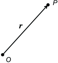
Figure 2.1: One body problem. Body $P$ with mass $M$ is assumed to be at rest at the origin $O$ of the coordinate system. The motion of a test particle, that is, of a body with negligible mass $m\ll M$ is then considered assuming that $m$ is so small that its influence on the body with mass $M$ can be totally neglected. Position of that test particle is denoted by $r$.

Here and below the absolute value of a vector is designated by the same symbol as the vector itself, but not in boldface (e.g., $r=|{\mbox{\boldmath$r$}}|$). In Newtonian mechanics force is equal to the product of the mass and acceleration of the particle. Therefore, one has

$${\mbox{\boldmath$F$}}=m\,{d^{2}{\mbox{\boldmath$r$}}\over dt^{2}}=m\,{\ddot{\mbox{\boldmath$r$}}}$$

(a dot over a symbol denote the time derivative of the corresponding quantity and a double dot the second time derivative), and finally the equations of motion of the mass $m$ read

$${\ddot{\mbox{\boldmath$r$}}}+GM\,{{\mbox{\boldmath$r$}}\over r^{3}}=0.$$ (2.1)

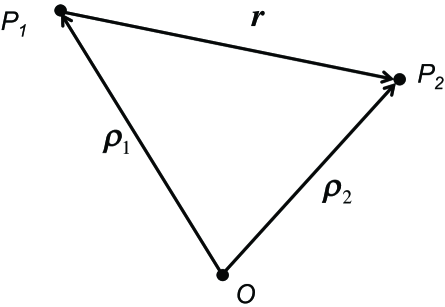
Figure 2.2: General two body problem. Bodies $P_{1}$ and $P_{2}$ with masses $m_{1}$ and $m_{2}$ have positions ${\mbox{\boldmath$\rho$}}_{1}$ and ${\mbox{\boldmath$\rho$}}_{2}$, respectively. The position of body $P_{2}$ relative to body $P_{1}$ is ${\mbox{\boldmath$r$}}={\mbox{\boldmath$\rho$}}_{2}-{\mbox{\boldmath$\rho$}}_{1}$. Point $O$ is the origin of the chosen coordinate system.

Let us now consider the general case of two bodies experiencing mutual gravitational attraction. Let vectors ${\mbox{\boldmath$\rho$}}_{1}$ and ${\mbox{\boldmath$\rho$}}_{2}$ are the positions of bodies $P_{1}$ and $P_{2}$ with masses $m_{1}$ and $m_{2}$, respectively, in some coordinate system, and ${\mbox{\boldmath$r$}}={\mbox{\boldmath$\rho$}}_{2}-{\mbox{\boldmath$\rho$}}_{1}$ is the position of body $P_{2}$ with respect to body $P_{1}$ (Fig. 2.2). Then, the equations of motions of the two bodies read

$$m_{1}\,{\ddot{\mbox{\boldmath$\rho$}}}_{1} = Gm_{1}m_{2}\,{{\mbox{\boldmath$r$}}\over r^{3}},$$

$$m_{2}\,{\ddot{\mbox{\boldmath$\rho$}}}_{2} =- Gm_{1}m_{2}\,{{\mbox{\boldmath$r$}}\over r^{3}}.$$ (2.2)

This is a system of differential equations of order 12 (we have a differential equation of order 2 for each of the 3 components of the two vectors ${\mbox{\boldmath$\rho$}}_{1}$ and ${\mbox{\boldmath$\rho$}}_{2}$, the equations being coupled to each other). Now, summing these two equations one gets that the following linear combination of the position vectors remains zero at any moment of time:

$$m_{1}\,{\ddot{\mbox{\boldmath$\rho$}}}_{1}+m_{2}\,{\ddot{\mbox{\boldmath$\rho$}}}_{2}=0.$$ (2.3)

Since the masses are considered to be constant in our consideration, this equation can be integrated twice:

$$m_{1}\,{\dot{\mbox{\boldmath$\rho$}}}_{1}+m_{2}\,{\dot{\mbox{\boldmath$\rho$}}}_{2}={\mbox{\boldmath$A$}},$$ (2.4)

$$m_{1}\,{\mbox{\boldmath$\rho$}}_{1}+m_{2}\,{\mbox{\boldmath$\rho$}}_{2}={\mbox{\boldmath$A$}}\,t+{\mbox{\boldmath$B$}},$$ (2.5)

where vectors $A$ and $B$ are some arbitrary integration constants. Clearly these equations express that the barycenter (center of mass) of the system of two bodies moves uniformly and rectilinear (that is, with a constant velocity proportional to $A$). The position of the barycenter is

$${\mbox{\boldmath$R$}}={m_{1}\,{\mbox{\boldmath$\rho$}}_{1}+m_{2}\,{\mbox{\boldmath$\rho$}}_{2}\over m_{1}+m_{2}},$$

so that one has

$${\dot{\mbox{\boldmath$R$}}}={{\mbox{\boldmath$A$}}\over m_{1}+m_{2}}={\rm const},$$

$${\mbox{\boldmath$R$}}={{\mbox{\boldmath$A$}}\over m_{1}+m_{2}}\ t+{{\mbox{\boldmath$B$}}\over m_{1}+m_{2}}.$$

Quantities which remain constant during the motion are called integrals of motion. Here we have found 6 integrals of motion (3 components of $A$ and 3 components of $B$). One often can use the integrals of motion to reduce the order of the system of differential equations describing the motion. Let us demonstrate that using (2.5) one can reduce the order of (2.1) by 6. Two ways of thinking are possible here. First, let us consider the motion of body $P_{2}$ relative body $P_{1}$. In this case we need an equation for $r$. Cancelling factors $m_{1}$ and $m_{2}$ in the first and second equation of (2.1), respectively,

$${\ddot{\mbox{\boldmath$\rho$}}}_{1} = Gm_{2}\,{{\mbox{\boldmath$r$}}\over r^{3}},$$

$${\ddot{\mbox{\boldmath$\rho$}}}_{2} =- Gm_{1}\,{{\mbox{\boldmath$r$}}\over r^{3}}$$

and subtracting the resulting equations one gets

$${\ddot{\mbox{\boldmath$r$}}}+G(m_{1}+m_{2})\,{{\mbox{\boldmath$r$}}\over r^{3}}=0.$$ (2.6)

This is a system of differential equations of order 6 ( components of $r$ are defined by a system of 3 coupled equations of order 2). Having a solution of this equation (that is, assuming that $r$ as a function of time is known) one has two linear equations for vectors ${\mbox{\boldmath$\rho$}}_{1}$ and ${\mbox{\boldmath$\rho$}}_{2}$:

$$m_{1}\,{\mbox{\boldmath$\rho$}}_{1}+m_{2}\,{\mbox{\boldmath$\rho$}}_{2} = {\mbox{\boldmath$A$}}\,t+{\mbox{\boldmath$B$}},$$

$${\mbox{\boldmath$\rho$}}_{2}-\,{\mbox{\boldmath$\rho$}}_{1} = {\mbox{\boldmath$r$}}.$$

The 6 constants $A$ and $B$ can be chosen arbitrarily (for example, computed from the initial values for the positions ${\mbox{\boldmath$\rho$}}_{1}$ and ${\mbox{\boldmath$\rho$}}_{2}$, and velocities ${\dot{\mbox{\boldmath$\rho$}}}_{1}$ and ${\dot{\mbox{\boldmath$\rho$}}}_{2}$).

Another possible way to use the integrals of motion (2.5) to reduce the order of (2.1) is to consider the motion of each body relative to the barycenter. This corresponds to choosing the coordinate system with the origin at the barycenter and setting ${\mbox{\boldmath$A$}}=0$ and ${\mbox{\boldmath$B$}}=0$. This is always possible due to the Galilean relativity principle stating that coordinate systems moving with a constant velocity relative to each other are equivalent and can be equally used to describe the motion. From

$$m_{1}\,{\mbox{\boldmath$\rho$}}_{1}+m_{2}\,{\mbox{\boldmath$\rho$}}_{2} = 0,$$

$${\mbox{\boldmath$\rho$}}_{2}-\,{\mbox{\boldmath$\rho$}}_{1} = r$$

one has

$${\mbox{\boldmath$\rho$}}_{2} = -\displaystyle{m_{2}\over m_{1}+m_{2}}\,{\mbox{\boldmath$r$}},$$

$${\mbox{\boldmath$\rho$}}_{1} = \displaystyle{m_{1}\over m_{1}+m_{2}}\,{\mbox{\boldmath$r$}}.$$

Substituting these two equations into (2.6) one gets two uncoupled equations for ${\mbox{\boldmath$\rho$}}_{1}$ and ${\mbox{\boldmath$\rho$}}_{2}$:

$${\ddot{\mbox{\boldmath$\rho$}}}_{1}+G{m_{2}^{3}\over(m_{1}+m_{2})^{2}}\,{{\mbox{\boldmath$\rho$}}_{1}\over\rho_{1}^{3}}=0,$$

$${\ddot{\mbox{\boldmath$\rho$}}}_{2}+G{m_{1}^{3}\over(m_{1}+m_{2})^{2}}\,{{\mbox{\boldmath$\rho$}}_{2}\over\rho_{2}^{3}}=0.$$ (2.7)

Note that the second equation in (2.1) can be derived from the first one by interchanging the indices $1\leftrightarrow 2$.

Now we notice that in all cases considered above the equations of motion (2.1), (2.6) and (2.1) have the form

$${\ddot{\mbox{\boldmath$r$}}}+\kappa^{2}\,{{\mbox{\boldmath$r$}}\over r^{3}}=0,$$ (2.8)

where $\kappa>0$ is a constant depending on the masses of the bodies. In the following we consider the equations of motion in their generic form (2.8).

Remark. Note that the same equation (2.8) describes also the position of any body of a system of $N$ bodies with $N>2$ when some special configuration (special set of positions and velocities) of the $N$ bodies is considered. Such a configuration must possess certain symmetry so that the sum of all gravitational forces acting on each of the $N$ bodies is always directed toward the center of mass of the $N$-body system. Such configurations are called central configurations.

Exercise. Find some examples of the central configuration. Hint: consider the bodies at the vertices of equilateral polygons.

2.2 Integrals of angular momentum and energy

Summary: Integral of angular momentum (the law of areas). The second Kepler’s law. Integral of energy. Integrals of angular momentum and energy in polar coordinates.

The equations (2.8) can be further simplified by using the so-called integrals of area (or angular momentum) and energy. Let us first compute the cross product of (2.8) by $r$:

$${\mbox{\boldmath$r$}}\times\left({\ddot{\mbox{\boldmath$r$}}}+\kappa^{2}\,{{\mbox{\boldmath$r$}}\over r^{3}}\right)=0$$

which implies

$${\mbox{\boldmath$r$}}\times{\ddot{\mbox{\boldmath$r$}}}=0.$$

The latter equation can be integrated to give

$${\mbox{\boldmath$r$}}\times{\dot{\mbox{\boldmath$r$}}}={\mbox{\boldmath$c$}},$$ (2.9)

where ${\mbox{\boldmath$c$}}={\rm const}$. Eq. (2.9) has two consequences:

1. The motion is planar. Indeed, the constant vector $c$ is orthogonal to both position vector $r$ and velocity vector $\dot{{\mbox{\boldmath$r$}}}$ at any moment of time. The last two vectors define the momentary plane of motion and since ${\mbox{\boldmath$c$}}={\rm const}$ this plane does not change.

2. The area swept out by position vector $r$ within an infinitely small interval of time $dt$ remains constant. Indeed, if at some moment of time $t$ the position vector is $r$ then at time $t+dt$ the position vector is ${\mbox{\boldmath$r$}}+{\dot{\mbox{\boldmath$r$}}}\,dt$, where ${\dot{\mbox{\boldmath$r$}}}$ is the velocity vector at time $t$. The area encompassed by vectors $r$ and ${\mbox{\boldmath$r$}}+{\dot{\mbox{\boldmath$r$}}}\,dt$ can be calculated as $dA={1\over 2}\,|{\mbox{\boldmath$r$}}\times({\mbox{\boldmath$r$}}+{\dot{\mbox{\boldmath$r$}}}\,dt)|={1\over 2}\,|{\mbox{\boldmath$r$}}\times{\dot{\mbox{\boldmath$r$}}}|\,dt={1\over 2}\,c\,dt$. Therefore, $\dot{A}={1\over 2}\,c={\rm const}$. This is nothing else than the second Kepler law in differential form (its usual integral form $\Delta A={1\over 2}\,c\,\Delta t$ immediately follows from the differential form $\dot{A}={1\over 2}\,c$). Let us remind that the standard formulation of the second Kepler’s law states that “a line joining a planet and the Sun sweeps out equal areas during equal intervals of time”.

Remark. We have used only one property of (2.8) in order to derive (2.9): the property that the force is proportional to $r$. The coefficient of proportionality plays no role here and can be any function of time $t$, position $r$, velocity $\dot{{\mbox{\boldmath$r$}}}$. Such forces are called central forces. Motion with any central forces is, therefore, planar and satisfies the second Kepler’s law.

Denoting the components of vectors as ${\mbox{\boldmath$r$}}=(x,y,z)$, ${\dot{\mbox{\boldmath$r$}}}=(\dot{x},\dot{y},\dot{z})$, ${\mbox{\boldmath$c$}}=(c_{x},c_{y},c_{z})$ one can rewrite (2.9) in the form

$$y\,\dot{z}-\dot{y}\,z=c_{x},$$

$$z\,\dot{x}-\dot{z}\,x=c_{y}, \,{}^{\prime}$$ (2.9)

$$x\,\dot{y}-\dot{x}\,y=c_{z},$$

Let us now use the fact that the motion is planar and re-orient our coordinates in such a way that one of the body’s coordinate remain identically zero. This means that the body remains in the plane $z=0$ of the coordinate system. Let us then denote the two other coordinates as $\xi$ and $\eta$. In these new coordinates Eq. (2.9) reads

$$\xi\,\dot{\eta}-\dot{\xi}\,\eta=c,$$ (2.10)

and the equations of motion can be rewritten as

$${\ddot{\xi}}+\kappa^{2}\,{\xi\over r^{3}}=0,$$

$${\ddot{\eta}}+\kappa^{2}\,{\eta\over r^{3}}=0$$ (2.11)

where $r=\sqrt{\xi^{2}+\eta^{2}}$.

Let us now multiply the first equation of (2.2) by $2\,{\dot{\xi}}$ and the second one by $2\,{\dot{\eta}}$, and then add the two resulting equations to get

$$2{\dot{\xi}}\,{\ddot{\xi}}+2{\dot{\eta}}\,{\ddot{\eta}}=-\kappa^{2}\,{2{\dot{\xi}}\,\xi+2{\dot{\eta}}\,\eta\over r^{3}}.$$

Both sides of the latter equation are total time derivatives. Integrating this equation one gets

$${\dot{\xi}}^{2}+{\dot{\eta}}^{2}=2\kappa^{2}\,{1\over r}+h,$$ (2.12)

where $h={\rm const}$ is a constant of integration. The validity of (2.12) can be checked by calculating its derivative with respect to time $t$ and comparing it with the previous equations. Quantity $h$ represents one more integral of motion which is called energy constant. Indeed, the left-hand side of (2.12) is doubled kinetic energy of the body per unit of mass and the right-hand side is minus doubled potential energy per unit of mass plus constant $h$.

Let us now introduce polar coordinates $r$ and $u$ instead of Cartesian coordinates $\xi$ and $\eta$. Using standard relations $\xi=r\,\cos u$ and $\eta=r\,\sin u$ which imply, for example,

$${\dot{\xi}}={\dot{r}}\,\cos u-r\,\sin u\,{\dot{u}},$$

$${\dot{\eta}}={\dot{r}}\,\sin u+r\,\cos u\,{\dot{u}}$$

one gets the integrals of area (2.10) and of energy (2.12) in polar coordinates

$$r^{2}\,\dot{u}=c,$$ (2.13)

$${\dot{r}}^{2}+r^{2}\,{\dot{u}}^{2}=2\kappa^{2}\,{1\over r}+h.$$ (2.14)

The equations of motion (2.2) can be also expressed in polar coordinates $r$ and $u$. One can show that the only non-trivial equation reads

$$\ddot{r}-r\,{\dot{u}}^{2}+{\kappa^{2}\over r^{2}}=0.$$ (2.15)

Exercise. Rewrite the equations of motion (2.2) in polar coordinates $r$ and $u$ explicitly. Show that that they can be expressed as a sum of derivatives of the integrals (2.13) and (2.14).

2.3 Possible Orbits

Summary: Conic sections as possible orbits in the two-body problem. The first Kepler’s law. Definitions of the semi-latus rectum, eccentricity and the argument of pericenter. Apocenter and pericenter. Apsidal line. Elliptical, parabolic, hyperbolic and rectilinear motions.

Our aim now is investigate the form of the orbits implies by (2.13) and (2.14). Since we are interested in the form of the orbits only, we can eliminate the time variable from the two equations. Eq. (2.13) implied that $\dot{u}=c\,r^{-2}$. Therefore, $\dot{r}={d\over dt}r={dr\over du}\,{du\over dt}={dr\over du}\,c\,r^{-2}$. Substituting this into (2.14) one gets

$$\left({dr\over du}\right)^{2}\,{c^{2}\over r^{4}}+r^{2}\,{c^{2}\over r^{4}}=2\kappa^{2}\,{1\over r}+h$$

and, therefore,

$$\left(-{c\over r^{2}}\right)^{2}\,\left({dr\over du}\right)^{2}=2\kappa^{2}\,{1\over r}+h-{c^{2}\over r^{2}}.$$

Now let us consider first the case $c\neq 0$. The previous equations can be rewritten in the form

$$\left(\,{d\sigma\over du}\,\right)^{2}=h+{\kappa^{4}\over c^{2}}-\sigma^{2},$$

where

$$\sigma={c\over r}-{\kappa^{2}\over c}.$$

Since the right-hand side of this equation is non-negative (as a square of a real number $d\sigma/du$) one has also $h+{\kappa^{4}\over c^{2}}-\sigma^{2}\geq 0$ or $h+{\kappa^{4}\over c^{2}}\geq\sigma^{2}$. Considering that $\sigma^{2}\geq 0$ one gets

$$h+{\kappa^{4}\over c^{2}}\geq 0.$$

Therefore, one can designate $\left(h+{\kappa^{4}\over c^{2}}\right)^{1/2}=A$, $A\geq 0$.

Exercise. Prove that for any position $r$ and velocity ${\dot{\mbox{\boldmath$r$}}}$ the integrals $h$ and $c$ take such values that $h+\kappa^{4}\,c^{-2}\geq 0$. Hint: use the definitions of $h$ and $c$ as functions of $r$ and ${\dot{\mbox{\boldmath$r$}}}$.

Therefore, one get the differential equation for the orbit

$$\left(\,{d\sigma\over du}\,\right)^{2}=A^{2}-\sigma^{2}.$$ (2.16)

Let us first consider the case $A\neq 0$. One can consider that $d\sigma/du>0$. The second case of $d\sigma/du<0$ can be derived from the first one by setting $u=-u$, that is by mirroring the first case. It is clear, however, that the orbit in both cases remains the same and it is only the direction in which the body moves along the orbit which changes. The direction of motion is not interesting for us for the moment. Therefore, the solution can be written as

$$u=\arccos{\sigma\over A}\,+\omega,$$

or

$$\sigma=A\cos(u-\omega),$$

$\omega={\rm const}$ being an arbitrary constant. Taking into account the definitions of $\sigma$ and $A$ one has

$$r={p\over 1+e\,\cos(u-\omega)},$$ (2.17)

where $p>0$ and $e\geq 0$ represent two parameters of the orbit defined through the integrals of motion $h$ and $c$ and parameter $\kappa$:

$$p={c^{2}\over\kappa^{2}},$$ (2.18)

$$e=\sqrt{1+h\,{c^{2}\over\kappa^{4}}}.$$ (2.19)

Remark. One can see that formally Eq. (2.16) has one more solution: $\sigma=\pm A$ which means that $r=p/(1\pm e)$ is constant. Using the equations of motion in polar coordinates (2.15) one can see that this is valid only when $A=0$ (this case is treated below separately). Indeed, a solution of equations of motion (e.g. a solution of (2.2)) must satisfy also the corresponding integrals of motion (e.g. (2.13)–(2.14)), but not any solution satisfying the integrals of motion also satisfy the equations of motion. That is, the integrals of motion are necessary, but not sufficient conditions for a function to be a solution of the equations of motion. Whether a function satisfying of the integrals of motion also satisfies the equations of motion should be checked explicitly. One can easily see that (2.17) is really a solution of (2.15), but $\sigma=\pm A\neq 0$ is not.

Eq. (2.17) shows that the orbit in this case (we assumed $c\neq 0$ and $A\neq 0$) is a conic section. The parameter $p>0$ is called semi-latus rectum and $e$ represents the eccentricity of the conic section. From (2.17) one sees that for $e<1$ (this corresponds to $h<0$) the orbit is an ellipse, for $e=1$ ($h=0$) a parabola and for $e>1$ ($h>0$) a hyperbola. This proves the first Kepler’s law: the orbit of every planet is an ellipse with the Sun at one of the two foci.

For any $e$ the polar angle $u$ can take the value $u=\omega$. In this case the denominator of (2.17) takes its maximal value $1+e$. Therefore, the radial distance $r$ is minimal at this point

$$r={p\over 1+e}=r_{\rm min}.$$

The point of the orbit where the distance $r$ takes its minimal value is called pericenter or periapsis (or perihelion when motion relative to the Sun is considered, or perigee when motion relative to the Earth is considered, or periastron when motion of a binary star is considered). The constant $\omega$ is called argument of pericenter.

For $e<1$, polar angle $u$ can also take the value $u=\omega+\pi$ ($\pi=3.14\dots$). Here the distance $r$ takes its maximal value

$$r={p\over 1-e}=r_{\rm max}.$$

The point of the elliptic orbit where the distance $r$ takes its maximal value is called apocenter or apoapsis (or aphel when motion relative to the Sun is considered, or apogee when motion relative to the Earth is considered, or apoastron when motion of a binary star is considered). Pericenter and apocenter are called apsides. A line connecting pericenter and apocenter is called line of apsides or apse line.

The mean distance of the body calculated as arithmetic mean of the maximal and minimal values of $r$ is called semi-major axis of the orbit:

$$a={1\over 2}\left(r_{\rm min}+r_{\rm max}\right)={p\over 1-e^{2}}$$

or

$$p=a\,(1-e^{2}).$$ (2.20)

Substituting (2.18) and (2.19) into (2.20) one gets the relation between $a$ and the integrals of motion:

$$a=-{\kappa^{2}\over h}.$$ (2.21)

One can see that $a$ depends only on $\kappa$ and the energy constant $h$, and not on $c$. Eqs. (2.20) and (2.21) represent definition of $a$ for any non-negative value of $e$ (or for any $h$ and $c$). From (2.21) it follows that $a$ is infinite for parabolic motion ($e=1$, $h=0$) and negative for hyperbolic one ($e>1$, $h>0$).

Let us consider now the two remained cases. First, for $c\neq 0$ and $A=0$ the differential equation for the orbit reads $\left(\,{d\sigma\over du}\,\right)^{2}=-\sigma^{2},$ which means that both $\sigma$ and ${d\sigma\over du}$ should be zero and therefore $\sigma\equiv 0$. This means that

$${c\over r}-{\kappa^{2}\over c}=0$$

and

$$r=p.$$ (2.22)

This solution coincides with (2.17) for $e=0$ (this agrees also with the definition of $e$: if $A=0$, one has $h=-\kappa^{4}/c^{2}$ and from (2.19) it follows that $e=0$).

Finally, if $c=0$ from (2.13) one gets $\dot{u}=0$ and therefore $u={\rm const}$, which means that the motion is rectilinear. Substituting this into the energy integral (2.14) one gets

$${\dot{r}}^{2}=2\kappa^{2}\,{1\over r}+h.$$

For $h<0$ the motion is bounded since both sides of the latter equations must be non-negative. For negative $h$ this means that $r\leq-{2\kappa^{2}\over h}>0$. This is rectilinear motion of elliptical kind (the elliptical motion with (2.17) with $h<0$ and $e<1$ is also bounded in space). For non-negative $h$ one can calculate the velocity of the body for infinite distance $r\to\infty$: $v_{\infty}=\lim_{r\to\infty}{\dot{r}}=\sqrt{h}$. For $h=0$ velocity goes to zero: $v_{\infty}=0$. For $h>0$ the velocity always remains positive: $v_{\infty}>0$. These are rectilinear motions of parabolic and hyperbolic kinds, respectively.

Exercise. For parabolic case $h=0$, one has ${\dot{r}}^{2}=2\kappa^{2}\,{1\over r}$. This equation has a simple analytical solution. Find this solution in its most general form.

2.4 Orbit in Space

Summary: Three Euler angles defining the orientation of the orbit in space: longitude of the ascending node, inclination and the argument of pericenter. The rotational matrix between inertial coordinates in space and the coordinates in the orbital plane.

Let us now consider the orientation of the orbit in space. Above we have seen that the orbit lies in a plane perpendicular to vector $c$. Let us consider two orthogonal Cartesian coordinate systems: (1) $(x,y,z)$ is some arbitrary inertial reference system where the equations of motion (2.8) are initially formulated and (2) $(X,Y,Z)$ is oriented in such a way that $XY$-plane contains the orbit (that is, axis $Z$ is parallel to vector $c$), and the pericenter of the orbit lies on axis $X$. The origins of both reference systems coincide and the transformation between these coordinates is a pure three-dimensional (time-independent) rotation. The rotation can be parametrized in a multitude of ways. Historically, it was parametrized by three Euler-type angles. Let us first consider the points where the orbit intersects the $xy$-plane. These points are called nodes. The node at which the body, in course of its motion, proceeds from the area of negative $z$ to that of positive $z$ is called ascending node. Let us introduce an intermediate coordinate system $(x_{1},y_{1},z_{1})$ that is obtained from $(x,y,z)$ by a rotation around axis $z=z_{1}$ so that axis $x_{1}$ contains the ascending node of the orbit:

$$\pmatrix{x_{1}\cr y_{1}\cr z_{1}}={\hbox{\bf A}}_{z}(\Omega)\,\pmatrix{x\cr y\cr z},$$ (2.23)

where ${\hbox{\bf A}}_{z}$ is the rotational matrix around $z$-axis

$${\hbox{\bf A}}_{z}(\alpha)=\pmatrix{\cos\alpha&\sin\alpha&0\cr-\sin\alpha&\cos\alpha&0\cr 0&0&1}.$$ (2.24)

Angle $\Omega$ is the called the longitude of the ascending node or simply longitude of the node. One more intermediate system $(x_{2},y_{2},z_{2})$ is obtained from $(x_{1},y_{1},z_{1})$ by a rotation around axis $x_{1}=x_{2}$ so that the direction of axis $z_{2}$ coincides with vector $c$:

$$\pmatrix{x_{2}\cr y_{2}\cr z_{2}}={\hbox{\bf A}}_{x}(i)\,\pmatrix{x_{1}\cr y_{1}\cr z_{1}}={\hbox{\bf A}}_{x}(i)\,{\hbox{\bf A}}_{z}(\Omega)\,\pmatrix{x\cr y\cr z},$$ (2.25)

where ${\hbox{\bf A}}_{x}$ is the rotational matrix around $x$-axis

$${\hbox{\bf A}}_{x}(\alpha)=\pmatrix{1&0&0\cr 0&\cos\alpha&\sin\alpha\cr 0&-\sin\alpha&\cos\alpha\cr}.$$ (2.26)

Angle $i$ is called inclination. Two angles – longitude of the node $\Omega$ and inclination $i$ – fully define the orientation of the orbital plane in space. The orbit lies in the $x_{2}y_{2}$-plane. Coordinates $(x_{2},y_{2})$ coincides with coordinates $(\xi,\eta)$ used above. The last step is to define the orientation of the orbit in the orbital plane. This is done by using argument of pericenter $\omega$. The final coordinate system $(X,Y,Z)$ can be obtained from $(x_{2},y_{2},z_{2})$ by a rotation around axis $z_{2}$:

$$\pmatrix{X\cr Y\cr Z}={\hbox{\bf A}}_{z}(\omega)\,\pmatrix{x_{2}\cr y_{2}\cr z_{2}}={\hbox{\bf A}}_{z}(\omega)\,{\hbox{\bf A}}_{x}(i)\,{\hbox{\bf A}}_{z}(\Omega)\,\pmatrix{x\cr y\cr z}\,.$$ (2.27)

In the following the inverse transformation plays an important role:

$$\pmatrix{x\cr y\cr z}={\hbox{\bf P}}\pmatrix{X\cr Y\cr Z}\,,$$ (2.28)

$${\hbox{\bf P}}={\hbox{\bf A}}^{T}_{z}(\Omega)\,{\hbox{\bf A}}^{T}_{x}(i)\,{\hbox{\bf A}}^{T}_{z}(\omega)\,.$$ (2.29)

Here superscript $T$ denotes the transpose of the corresponding matrix. Note that for any rotational matrix ${\hbox{\bf R}}^{T}={\hbox{\bf R}}^{-1}$. Explicitly one has:

P $$= \left(\begin{array}[]{rrr}\cos\Omega\,\cos\omega-\sin\Omega\,\cos i\,\sin\omega&-\cos\Omega\,\sin\omega-\sin\Omega\,\cos i\,\cos\omega&\sin\Omega\,\sin i\\ \quad\sin\Omega\,\cos\omega+\cos\Omega\,\cos i\,\sin\omega&\quad-\sin\Omega\,\sin\omega+\cos\Omega\,\cos i\,\cos\omega&\quad-\cos\Omega\,\sin i\\ \sin i\,\sin\omega&\sin i\,\cos\omega&\cos i\end{array}\ \right)\,.$$ (2.33)

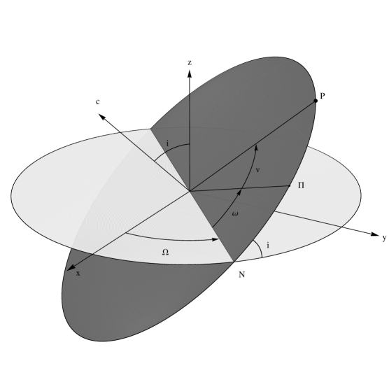
Figure 2.3: Orbit in space. The picture shows the definition of three Euler-like angles $\Omega$, $i$ and $\omega$ that fully describe the orientation of the orbit of a two-body problem in space. $N$ is the ascending node, $\Pi$ is the pericenter, $P$ is the position of the body. One more angle (true anomaly $v$) defines the position of the body on the orbit.

2.5 Kepler Equation

Summary: True Anomaly. Kepler equation in true anomaly. Eccentric anomaly. Various relations between the true and eccentric anomaly. Kepler equation in eccentric anomaly. Mean anomaly. The period of motion and the third Kepler law.

The true anomaly $v$ is defined as $v=u-\omega$. Since $\omega={\rm const}$ one has $\dot{v}=\dot{u}$. Therefore, integral of areas (2.13) can be written as

$$\dot{v}=c=\kappa\,\sqrt{p}\,{1\over r^{2}}.$$

Using (2.17) one gets

$${dv\over(1+e\,\cos v)^{2}}=\kappa\,p^{-3/2}\,dt\,,$$ (2.35)

which after integration gives the Kepler equation in true anomaly

$$\kappa\,p^{-3/2}\,t=\int{dv\over(1+e\,\cos v)^{2}}+{\rm const}\,.$$

In this Section from now on we consider only the case of elliptical motion with $e<1$. The integral above cannot be computed analytically. In order to simplify the computations one introduces the so-called eccentric anomaly. The eccentric anomaly $E$ is defined by its relation to the true anomaly $v$:

$$\cos v={\cos E-e\over 1-e\,\cos E},$$ (2.36)

It is easy to calculate $\sin^{2}v$ from this equation. Choosing the sign so that $E=v$ for $e=0$ one gets

$$\sin v={\sqrt{1-e^{2}}\,\sin E\over 1-e\,\cos E}.$$ (2.37)

Solving (2.36) for $\cos E$ one gets

$$\cos E={\cos v+e\over 1+e\,\cos v},$$ (2.38)

so that

$$1-e\,\cos E={1-e^{2}\over 1+e\,\cos v},$$ (2.39)

which together with (2.37) gives

$$\sin E={\sqrt{1-e^{2}}\,\sin v\over 1+e\,\cos v}.$$ (2.40)

It is easy to see that (2.38) and (2.40) can be obtained from (2.36) and (2.37) by making the substitution $(E,v,e)\,\longrightarrow\,(v,E,-e)$. From (2.36) and (2.37) one can derive a relation between $v$ and $E$ which is convenient for numerical calculations

$$\tan{v\over 2}=\sqrt{1+e\over 1-e}\,\tan{E\over 2}.$$ (2.41)

From this equation it is easy to see that $E$ and $v$ are equal at apsides.

Now let us express the Kepler equation (2.35) in terms of the eccentric anomaly. Taking a derivative of (2.39) one gets

$$\sin E\ dE={(1-e^{2})\,\sin v\over(1+e\,\cos v)^{2}}\,dv,$$

which together with (2.37) gives

$${dv\over(1+e\,\cos v)^{2}}=(1-e^{2})^{-3/2}\,(1-e\,\cos E)\,dE.$$

Substituting this into (2.35) one gets

$$(1-e\,\cos E)\,dE=\kappa\,a^{-3/2}\,dt$$ (2.42)

or after integrating

$$E-e\,\sin E=M,$$ (2.43)

where $M=n(t-T)$ is the mean anomaly, $n=\kappa\,a^{-3/2}$ is the mean motion, and $T$ is an integration constant representing the moment time at which $M=0$. It is easy to see from (2.43) and (2.41) that for $t=T$ one has $M=E=v=0$ and the body is situated in its pericenter. However, for $e=0$ the orbit is circular so that any point can be declared to be pericenter. That is why, the definition of the mean anomaly is often taken to be $M=M_{0}+n(t-t_{0})$, where $M_{0}$ is the value of the mean anomaly at some moment $t=t_{0}$.

The period of motion $P$ an be defined as a time interval between two successive pericenters ($M=0$ and $M=2\pi$). Then it is clear that $P={2\pi\over n}$, which can be re-written as

$${P^{2}\over a^{3}}={4\pi\over\kappa^{2}}={\rm const}.$$

This is the third Kepler’s law: the square of the orbital period of a planet is directly proportional to the cube of the semi-major axis of its orbit. However, the constant $\kappa$ depends on the masses of both bodies of the two-body problem. Considering the motion of two planets relative to the Sun in the framework of the two-body problem we have two different constants $\kappa_{i}$ entering the corresponding equations of motion of each of the two planets $\kappa^{2}_{i}=G\,(m_{\rm Sun}+m_{i})$. Hence, one gets the third Kepler’s law in its correct form

$$\left({P_{1}\over P_{2}}\right)^{2}=\left({a_{1}\over a_{2}}\right)^{3}\,{m_{\rm Sun}+m_{1}\over m_{\rm Sun}+m_{2}}$$

In the Solar system $m_{i}/m_{\rm Sun}<10^{-3}$ and the last factor is almost unity.

Using the eccentric anomaly $E$ it is easy to calculate the position and velocity of the object in two-body motion. For the position one has (here we use the known expressions of the true anomaly $v$ and relation (2.36)–(2.37)):

$$r = {p\over 1+e\,\cos v}=a\,(1-e\,\cos E),$$ (2.44)

$$X = r\,\cos v=a\,(\cos E-e),$$ (2.45)

$$Y = r\,\sin v=a\,\sqrt{1-e^{2}}\sin E.$$ (2.46)

Differentiating (2.45)–(2.46) with respect to time $t$ and using that

$$\dot{E}={n\over 1-e\,\cos E}$$ (2.47)

(the latter equation can be derived by differentiating the Kepler equation (2.43)) one gets

$$\dot{X} = -{a\,n\,\sin E\over 1-e\,\cos E},$$ (2.48)

$$\dot{Y} = {a\,\sqrt{1-e^{2}}\,n\,\cos E\over 1-e\,\cos E}.$$ (2.49)

We have now all formulas that are necessary to compute the position and velocity of a body in two-body motion. These calculations can be performed if eccentric anomaly $E$ is known as a function of time $t$. The relation between $E$ and $t$ is given by the Kepler equation (2.43). However, the latter equation is transcendent and cannot be solved algebraically. Let us turn to the analysis of the Kepler equation.

2.6 Solving the Kepler Equation

Summary: Existence and uniqueness of the solution. Iterative solution. Newtonian solution.

Let us confine ourselves by the case of elliptic motion with $0\leq e<1$. The Kepler equation $E-e\sin E=M$ can be considered as an implicit function $E(M)$ or as explicit function $M(E)$ ($e$ being a parameter in both cases).

1. $E(M)$ is a continuous function as an inverse function to a continuous function $M(E)$.

2. Since $|E-M|=e\,|\sin E|<1$ one has

   $$\lim_{E\to+\infty}M(E) = +\infty,$$

   $$\lim_{E\to-\infty}M(E) = -\infty.$$

From properties 1 and 2 follows that for any $M$ there exists at least one $E$ such that the Kepler equation is satisfied.

1. Since $\displaystyle{dM\over dE}=1-e\,\cos E>0$, $M(E)$ is monotone, and therefore, $E(M)$ is also monotone (as an inverse function of $M(E)$).

From these three properties it follows that for any $M$ there exists only one $E$ such that $E-e\,\sin E=M$.

Let us now consider how one can solve the Kepler equation. Generally we have a transcendent equation

$$f(x)=0,$$

that should be solved numerically. Moreover, we just have proved that in case of the Kepler equation one has only one solution for any $0\leq e<1$ and any $M$. Many numerical methods to find the solution are known. Let us consider two simplest methods which, however, are sufficient in many cases.

1. Iterations

   The method consists in starting with some initial value for $x$ (say $x_{0}$) and iterating the formula $x_{i+1}=x_{i}-f(x_{i})$ until the subsequent values of $x$ ($x_{i}$ and $x_{i+1}$) are close enough to each other: if $|x_{i+1}-x_{i}|<\varepsilon$, then $x_{i+1}$ is a solution of $f(x)=0$ such that $|f(x_{i})|<\varepsilon$. Convergence of the iterative sequence is guaranteed if the derivative $f^{\prime}(x)$ of $f(x)$ satisfies the inequality $|f^{\prime}(x)-1|<1$ (Schwarz, 1993). One can easily show that this inequality holds in case of the Kepler equation with $e<1$. In general, the convergence also depends on the starting point $x_{0}$.

   For the Kepler equation one gets $f(E)=E-e\,\sin E-M$ and the algorithm can be written as

   $$E_{0} = M,$$

   $$E_{i+1} = M+e\,\sin E_{i},\quad i=0,1,\dots$$

   One can prove that the initial condition $E_{0}=M$ guarantees that the iterations converge for any $e$ and $M$.

   
   

2. Newton’s method

   Another well-known method is the Newton’s (or Newton-Raphson) one. Again starting from some initial value for the root’s estimate $x_{0}$ one iterates $x_{i+1}=x_{i}-f(x_{i})/f^{\prime}(x_{i})$, where $f^{\prime}(x)$ is the derivative of $f(x)$. Again if $|x_{i+1}-x_{i}|<\varepsilon$, then $x_{i}$ is a solution of $f(x)=0$ with the corresponding accuracy. Convergence of the iterative sequence is guaranteed if the initial guess $x_{0}$ lies close enough to the root (Section 9.4 of Press et al. 1992).

   For the Kepler equation this implies the scheme

   $$E_{0} = M,$$

   $$E_{i+1} = \displaystyle{M+e\,\left(\sin E_{i}-E_{i}\,\cos E_{i}\right)\over 1-e\,\cos E_{i}},\quad i=0,1,\dots$$

   Again one can prove that the initial condition $E_{0}=M$ guarantees that the iterations converge for any $e$ and $M$. It is well known that if the initial guess of the rule is good enough, the Newton’s method converges much faster than the iteration method.

2.7 Hyperbolic and Parabolic Motion

Summary: The eccentric anomaly and the Kepler equation for the hyperbolic motion. Explicit solution for the parabolic motion.

When we introduced the eccentric anomaly $E$ and discussed the Kepler equation above we have concentrated on elliptic motion with eccentricity $0\leq e<1$. Let us now consider two other cases: hyperbolic motion with $e>1$ and parabolic one with $e=1$. The formula for the form of the orbit

$$r={p\over 1+e\,\cos v}$$

remains valid for any $e$. Let us first consider the case of hyperbolic motion with $e>1$. The semi-latus rectum is non-negative $p=a(1-e^{2})={c^{2}\over\kappa^{2}}>0$ (the case $c=0$ leads to the rectilinear motion, has been considered above and will not be considered here). But $e=\sqrt{1+h\,{c^{2}\over\kappa^{4}}}$ and, therefore, $e>1$ implies $h>0$, i.e. the total energy of the two-body system is positive. Since $a=-{\kappa^{2}\over h}$, $h>0$ implies in turn that the semi-major axis is negative $a<0$.

If one takes the transformations (2.38) and (2.40) relating sine and cosine of the eccentric one $E$ to the sine and cosine of the true anomaly $v$, it is easy to see that $\sin E$ is imaginary and $\cos E$ is real, but can exceed unity. Therefore, for hyperbolic motion $E$ is imaginary. One can continue in this way and work directly with complex numbers, but it is not convenient. We, therefore, try to make all our equations real again (as it is in the case of elliptical motion). To this end we define a new anomaly instead of $E$. Since

$$e^{\buildrel\circ\over{\hbox{\rm\char 16\relax}}x}=\cos x+\buildrel\circ\over{\hbox{\rm\char 16\relax}}\sin x,$$

$\buildrel\circ\over{\hbox{\rm\char 16\relax}}$ being imaginary unit, one has

$$\cos x={1\over 2}\,\left(e^{\buildrel\circ\over{\hbox{\rm\char 16\relax}}x}+e^{-\buildrel\circ\over{\hbox{\rm\char 16\relax}}x}\right),\quad\sin x={1\over 2\buildrel\circ\over{\hbox{\rm\char 16\relax}}}\,\left(e^{\buildrel\circ\over{\hbox{\rm\char 16\relax}}x}-e^{-\buildrel\circ\over{\hbox{\rm\char 16\relax}}x}\right),$$

and for $x=\buildrel\circ\over{\hbox{\rm\char 16\relax}}\,y$ one gets

$$\cos\buildrel\circ\over{\hbox{\rm\char 16\relax}}\,y = \cosh y,$$

$$\sin\buildrel\circ\over{\hbox{\rm\char 16\relax}}\,y = \buildrel\circ\over{\hbox{\rm\char 16\relax}}\,\sinh y.$$

Using these formulas one can introduce a new anomaly $H$ defined as $H=\buildrel\circ\over{\hbox{\rm\char 16\relax}}E$, so that

$$\cos E = \cosh H,$$

$$\sin E = -\buildrel\circ\over{\hbox{\rm\char 16\relax}}\sinh H.$$

This allows one to re-write Eq. (2.44)–(2.46) as

$$r = {p\over 1+e\,\cos v}=a\,(1-e\,\cos E)=|a|\,(e\,\cosh H-1),$$ (2.50)

$$X = r\,\cos v=a\,(\cos E-e)=|a|\,(e-\cosh H),$$ (2.51)

$$Y = r\,\sin v=a\,\sqrt{1-e^{2}}\sin E=|a|\,\sqrt{e^{2}-1}\,\sinh H,$$ (2.52)

and the Kepler equation (2.43) as

$$e\,\sinh H-H=M_{\rm hyp},$$ (2.53)

$$M_{\rm hyp}=\kappa\,|a|^{-3/2}\,(t-T).$$ (2.54)

The signs in (2.52) and (2.53) are chosen so that the body moves in the positive direction of the $Y$-axis for $t=T$. Eq. (2.53) is the Kepler equation for hyperbolic motion. It has only one solution for any value of mean anomaly $M_{\rm hyp}$.

Let us now consider the simple case of parabolic motion. Parabolic motion corresponds to $e=1$ and this implies that the total energy of the system is zero: $h=0$. The equation for the form of the orbit can be simplified to

$$r={p\over 1+\cos v}=q\,(1+\sigma^{2}),$$

where $\sigma=\tan{v\over 2}$ and $q=p/2$ is the perihelion distance of the parabolic orbit (since in the perihelion one has $v=0$ and $r=p/2$). From the definition of $\sigma$ one has

$$\sin v={2\sigma\over 1+\sigma^{2}},\quad\cos v={1-\sigma^{2}\over 1+\sigma^{2}}.$$

Therefore, the distance and coordinates of the body on a parabolic orbit can be written as

$$r = q\,(1+\sigma^{2}),$$ (2.55)

$$X = r\,\cos v=q\,(1-\sigma^{2}),$$ (2.56)

$$Y = r\,\sin v=2\,q\,\sigma.$$ (2.57)

Now, using the integral of angular momentum one gets

$$r^{2}\dot{v}=c=\kappa\,\sqrt{p}=\kappa\,\sqrt{2\,q}$$

and, therefore,

$$\dot{v}=\kappa\,\sqrt{2}\,q^{-3/2}\,(1+\sigma^{2})^{-2}.$$ (2.58)

Since $\sigma=\tan{v\over 2}$ we have

$${d\sigma\over dv}={1\over 2}\,(1+\sigma^{2}).$$

Integrating this equation and using (2.58) one gets

$${1\over 3}\sigma^{3}+\sigma=M_{\rm par},$$ (2.59)

$$M_{\rm par}={\kappa\over\sqrt{2}}\,q^{-3/2}\,(t-T).$$ (2.60)

Eq. (2.59) is the Kepler equation for parabolic motion. This equation can be solved analytically using, e.g., the well-known Kardan formulas. Indeed, the equation has only one real solution for any value of $M_{\rm par}$

$$\sigma = {1\over 2}\,Q^{1/3}-2\,Q^{-1/3},$$

$$Q = 12\,M_{\rm par}+4\,\sqrt{4+9\,M_{\rm par}^{2}}.$$ (2.61)

Note that for any $M_{\rm par}$ value of $Q$ remains positive. This means that the parabolic motion can be represented by an explicit analytical formula (this can be also done for circular motion with $e=0$ and for rectilinear motion of parabolic type with $c=0$ and $h=0$).

Exercise. Write the explicit formulas for the coordinates for the case $e=0$.

2.8 Relation between Position, Velocity and the Kepler Elements

Summary: Calculation of position and velocity from the Kepler elements. Calculation of the Kepler elements from the position and velocity. Orbit determination (an overview).

We have seen above that there are two equivalent ways to represent a particular two body motion: (1) to specify the initial conditions for the equation of motion, i.e. the position and velocity vectors ${\mbox{\boldmath$r$}}=(x,y,z)$ and ${\dot{\mbox{\boldmath$r$}}}=(\dot{x},\dot{y},\dot{z})$ together with the corresponding moment of time $t_{0}$ and the parameter $\kappa$, and (2) to fix the whole set of the six Kepler elements $a$, $e$, $i$, $\omega$, $\Omega$, $M_{0}=M(t_{0})$ again together with the moment of time $t_{0}$ for which the mean anomaly $M_{0}$ is supposed to be known and the parameter $\kappa$. Very often in the practical calculation one wants to switch between these two representations, that is to transform the position and velocity into the corresponding Kepler elements or vice verse. Here we give the set of formulas enabling one to perform these transformations for the case of elliptic motion.

The transformation from the Kepler elements to the position and velocity vectors can be done in the following way:

1. calculate mean motion as $n=\kappa\,a^{-3/2}$ and mean anomaly as $M=n\,(t-t_{0})+M_{0}$ (here the position and velocity vectors can be calculated for any arbitrary moments of time $t$, not necessarily for the moment $t_{0}$ for which the mean anomaly $M_{0}$ is specified),

2. calculate eccentric anomaly $E$ from $E-e\sin E=M$,

3. calculate position and velocity in the orbital plane:

   $$X = a\,(\cos E-e),$$

   $$Y = a\,\sqrt{1-e^{2}}\,\sin E,$$

   $$\dot{X} = -{a\,n\,\sin E\over 1-e\,\cos E},$$

   $$\dot{Y} = {a\,n\,\sqrt{1-e^{2}}\,\cos E\over 1-e\,\cos E},$$

4. calculate the position and velocity vectors in space as

   $$\pmatrix{x\cr y\cr z} = P\,\pmatrix{X\cr Y\cr 0},$$

   $$\pmatrix{\dot{x}\cr\dot{y}\cr\dot{z}} = P\,\pmatrix{\dot{X}\cr\dot{Y}\cr 0},$$

   where $P={\hbox{\bf A}}^{T}_{z}(\Omega)\,{\hbox{\bf A}}^{T}_{x}(i)\,{\hbox{\bf A}}^{T}_{z}(\omega)$ defined by (2.33).

The transformation from the position and velocity vectors to the Kepler elements is a bit more complicated and can be done as follows:

1. from the integrals of the areas ${\mbox{\boldmath$r$}}\times{\dot{\mbox{\boldmath$r$}}}={\mbox{\boldmath$c$}}$ one gets ${\mbox{\boldmath$c$}}=(c_{x},c_{y},c_{z})$

   $$c_{x} = y\,\dot{z}-\dot{y}\,z,$$

   $$c_{y} = z\,\dot{x}-\dot{z}\,x,$$

   $$c_{z} = x\,\dot{y}-\dot{x}\,y,$$

   $$c = |{\mbox{\boldmath$c$}}|=\sqrt{c_{x}^{2}+c_{y}^{2}+c_{z}^{2}}.$$

   Then the semi-latus rectum can be calculated as

   $$p={c^{2}\over\kappa^{2}},$$

   and from

   $$\pmatrix{c_{x}\cr c_{y}\cr c_{z}}={\hbox{\bf A}}^{T}_{z}(\Omega)\,{\hbox{\bf A}}^{T}_{x}(i)\,\pmatrix{0\cr 0\cr c}=\left(\begin{array}[]{rrr}c\sin i\sin\Omega\\ -c\sin i\cos\Omega\\ c\,\cos i\end{array}\right)$$ (2.65)

   which gives us three equations. The third equation can be written as

   $$\cos i={c_{z}\over c}$$ (2.66)

   and since $0\leq i\leq\pi$ this one equation is sufficient to calculate the inclination $i$. The two other equations read

   $$\sin\Omega = {c_{x}\over\sqrt{c_{x}^{2}+c_{y}^{2}}},$$

   $$\cos\Omega = -{c_{y}\over\sqrt{c_{x}^{2}+c_{y}^{2}}}$$ (2.67)

   and allow one to calculate $\Omega$. Note that if $c_{x}^{2}+c_{y}^{2}=0$, the inclination $i=0$ and $\Omega$ is not defined.

2. From Eq. (2.17) and $v=u-\omega$ one gets two equations

   $$e\,\cos v = {p\over r}-1,$$

   $$e\,\sin v = {\sqrt{p}\over\kappa}\,{{\mbox{\boldmath$r$}}\cdot{\dot{\mbox{\boldmath$r$}}}\over r}$$ (2.68)

   which can be used to calculate both the eccentricity $e$ and the true anomaly $v$. Then using (2.41) one can calculate the eccentric anomaly $E$, and from (2.43) the mean anomaly $M$. All these values of anomalies $v$, $E$ and $M$ correspond to time $t_{0}$ for which the position and velocity of the body is specified. Finally, from $p$ and $e$ it is easy to calculate the semi-major axis as $a=p\,{(1-e^{2})}^{-1}$;

3. From

   $$\pmatrix{x\cr y\cr z}={\hbox{\bf A}}^{T}_{z}(\Omega)\,{\hbox{\bf A}}^{T}_{x}(i)\,\pmatrix{r\cos(v+\omega)\cr r\sin(v+\omega)\cr 0}$$

   one gets

   $$\cos(v+\omega) = {x\over r}\,\cos\Omega+{y\over r}\,\sin\Omega,$$

   $$\sin(v+\omega) = \left(-{x\over r}\,\sin\Omega+{y\over r}\,\cos\Omega\right)\,\cos i+{z\over r}\,\sin i.$$ (2.69)

   From these two equations one calculates the angle $v+\omega$ and since $v$ is known, the argument of perihelion $\omega$.

2.9 Series Expansions in Two-Body Problem

Summary: Series in powers of time. Fourier series in multiples of the mean anomaly. Series in powers of the eccentricity.

As we have seen above a fully analytical solution of the two-body problem is impossible: one has a transcendent Kepler equation cannot be solved analytically. The only possibility to get an analytical solution is to use some kind of expansions. Below we consider three types of expansions which are widely used in celestial mechanics.

2.9.1 Taylor expansions in powers of time

The first kind of expansion is the Taylor expansion in powers of time. Let us consider the positional vector $r$ and expand it into Taylor series

$${\mbox{\boldmath$r$}}(t+\tau)=\sum_{k=0}^{\infty}{1\over k!}\,{\mbox{\boldmath$r$}}^{(k)}(t)\,\tau^{k},$$ (2.70)

where ${\mbox{\boldmath$r$}}^{(k)}$ are the derivatives of $r$ of order $k$. For $k=0$ and $k=1$ they represent the initial conditions for the motion ${\mbox{\boldmath$r$}}^{(0)}(t)={\mbox{\boldmath$r$}}(t)$ and ${\mbox{\boldmath$r$}}^{(1)}(t)={\dot{\mbox{\boldmath$r$}}}(t)$. Using the equation of motion

$${\ddot{\mbox{\boldmath$r$}}}=-\kappa^{2}\,{{\mbox{\boldmath$r$}}\over r^{3}}$$

it is clear that the higher derivatives for $k\geq 2$ can be calculated in terms of $r$ and ${\dot{\mbox{\boldmath$r$}}}$. E.g.,

$${\mbox{\boldmath$r$}}^{(2)} = {\ddot{\mbox{\boldmath$r$}}}=-\kappa^{2}\,S^{-3/2}\,{\mbox{\boldmath$r$}},$$

$${\mbox{\boldmath$r$}}^{(3)} = {3\over 2}\,\kappa^{2}\,S^{-5/2}\,{\dot{S}}\,{\mbox{\boldmath$r$}}-\kappa^{2}\,S^{-3/2}\,{\dot{\mbox{\boldmath$r$}}},$$ (2.71)

and so on. Here $S=r^{2}$, ${\dot{S}}=2\,{\mbox{\boldmath$r$}}\cdot\dot{{\mbox{\boldmath$r$}}}$, and the second- and higher-order derivatives of $S$ appearing in ${\mbox{\boldmath$r$}}^{(k)}$ for $k\geq 4$ can be calculated using

$$\ddot{S}=2\,h+2\kappa^{2}\,S^{-1/2},$$

where $h={\dot{\mbox{\boldmath$r$}}}\cdot{\dot{\mbox{\boldmath$r$}}}-{2\kappa^{2}\over r}$ is the energy integral. Therefore, it is clear that ${\mbox{\boldmath$r$}}(t+\tau)$ can be represented as a linear combination of ${\mbox{\boldmath$r$}}(t)$ and ${\dot{\mbox{\boldmath$r$}}}(t)$

$${\mbox{\boldmath$r$}}(t+\tau)=F\,{\mbox{\boldmath$r$}}(t)+G\,{\dot{\mbox{\boldmath$r$}}}(t),$$ (2.72)

while the functions $F$ and $G$ can be expanded in their Taylor series in powers of $\tau$:

$$F=\sum_{k=0}^{\infty}{1\over k!}\,F_{k}\,\tau^{k},$$

$$G=\sum_{k=0}^{\infty}{1\over k!}\,G_{k}\,\tau^{k}.$$ (2.73)

The coefficients $F_{k}$ and $G_{k}$ are functions of $\kappa$, $h$, $S$ and $\dot{S}$ only, and, therefore, can be calculated from the initial conditions ${\mbox{\boldmath$r$}}(t)$ and ${\dot{\mbox{\boldmath$r$}}}(t)$. Comparing (2.72)–(2.73) to (2.70) one gets for any $k$

$${\mbox{\boldmath$r$}}^{(k)}=F_{k}\,{\mbox{\boldmath$r$}}+G_{k}\,{\dot{\mbox{\boldmath$r$}}}.$$ (2.74)

Taking the derivative of (2.74) and comparing again with (2.74) written for $k+1$

$${\mbox{\boldmath$r$}}^{(k+1)}=F_{k+1}\,{\mbox{\boldmath$r$}}+G_{k+1}\,{\dot{\mbox{\boldmath$r$}}}$$

one gets the recursive formulas for $F_{k}$ and $G_{k}$:

$$F_{k+1}=\dot{F}_{k}-\kappa^{2}\,S^{-3/2}\,G_{k},$$ (2.75)

$$G_{k+1}=F_{k}+\dot{G}_{k}.$$ (2.76)

The initial conditions for (2.75)–(2.76) can be derived by considering the zero-order expansion ${\mbox{\boldmath$r$}}(t+\tau)={\mbox{\boldmath$r$}}(t)+{\cal O}(\tau)$:

$$F_{0}=1,$$ (2.77)

$$G_{0}=0.$$ (2.78)

Using (2.75)–(2.76) with (2.77)–(2.78) one gets, for example,

$$F_{1} = 0,$$

$$G_{1} = 1,$$

$$F_{2} = -\kappa^{2}\,S^{-3/2},$$

$$G_{2} = 0,$$

$$\dots$$ (2.79)

A detailed analysis of the two-body function by means of the complex analysis shows that the convergence of the derived series is guaranteed only for $|\tau|$ smaller than some limit depending on parameters of motion:

$$|\tau|<{1\over\kappa}\,q^{3/2}\,\alpha(e),$$ (2.80)

where $q$ is the perihelion distance, $e$ is the eccentricity and

$$\alpha(e)=\left[\begin{array}[]{ll}(1-e)^{-3/2}\,\left(\log\displaystyle{1+\sqrt{1-e^{2}}\over e}-\sqrt{1-e^{2}}\right),&e\leq 1\\[14.22636pt] (e-1)^{-3/2}\,\left(\sqrt{e^{2}-1}-\arctan\sqrt{e^{2}-1}\right),&e>1\end{array}\right.$$ (2.83)

Note that $\alpha(e)$ is a continuous monotone function for $e\geq 0$ and

$$\lim_{e\to 0}\alpha(e) = \infty,$$

$$\lim_{e\to 1}\alpha(e) = {2\sqrt{2}\over 3},$$

$$\lim_{e\to\infty}\alpha(e) = 0.$$

This means that the convergence is guaranteed for any $\tau$ if and only if the eccentricity of the orbit is zero and that the higher the eccentricity is the lower is the maximal $\tau$ for which the series in powers of time converge.

2.9.2 Fourier expansions in multiples of the mean anomaly

It is well known that any continuous complex function $f(x)$ of a real argument $x$ with a period of $2\pi$ (i.e. $f(x+2\pi)=f(x)$ for any $x$) can be expanded into Fourier series

$$f(x) = \sum_{k=-\infty}^{+\infty}\,f_{k}\,e^{\buildrel\circ\over{\hbox{\rm\char 16\relax}}\,k\,x},$$

$$f_{k} = {1\over 2\pi}\,\int_{0}^{2\pi}f(x)\,e^{-\buildrel\circ\over{\hbox{\rm\char 16\relax}}\,k\,x}\,dx,$$ (2.84)

which converges for any $x$. This kind of expansions can also be applied to the two-body problem. If $f(x)$ has additional properties (i.e., real or odd) formula (2.9.2) can be simplified. A nice overview of all special cases can be found in Chapter 12 of Press et al. (1992).

Let us consider function $f(E)=e\,\sin E$. This function is obviously real and odd ($f(-E)=-f(E)$). Therefore, the Fourier expansion can be simplified to be

$$E = M+e\,\sin E=M+\sum_{k=1}^{\infty}a_{k}\sin kM,$$ (2.85)

$$a_{k} = {2\over\pi}\,\int_{0}^{\pi}e\,\sin E\,\sin kM\,dM={2\over k}\,J_{k}(k\,e),$$ (2.86)

where $J_{n}(x)$ are the Bessel functions of the first kind defined as

$$J_{n}(x)={1\over\pi}\,\int_{0}^{\pi}\cos\left(n\,\theta-x\,\sin\theta\right)\,d\theta.$$ (2.87)

Many properties of $J_{n}(x)$ can be found e.g. in Chapter 9 of Abramowitz & Stegun (1965).

Exercise. Prove the second equality in (2.86) by taking the integral by parts.

Therefore,

$$E = M+\sum_{k=1}^{\infty}{2\over k}\,J_{k}(k\,e)\,\sin kM.$$ (2.88)

To give one more example let us note that

$${a\over r}={1\over n}\,\dot{E}\,.$$

Therefore, taking a derivative of (2.88) one gets

$${a\over r} = 1+\sum_{k=1}^{\infty}2\,J_{k}(k\,e)\,\cos kM.$$ (2.89)

In general one has

$$\left({r\over a}\right)^{n}\,e^{\buildrel\circ\over{\hbox{\rm\char 16\relax}}\,m\,v} = \sum_{k=-\infty}^{\infty}X_{k}^{n,m}(e)\,e^{\buildrel\circ\over{\hbox{\rm\char 16\relax}}\,k\,M},$$ (2.90)

where $X_{k}^{n,m}(e)$ are a three-parametric family of functions called Hansen coefficients.

2.9.3 Taylor expansions in powers of the eccentricity

The third kind of expansions are series in powers of eccentricity $e$. Let us consider these series for the example of the eccentric anomaly. Re-writing the Kepler equation in the form

$$E=M+e\sin E,$$ (2.91)

one has iteratively

$$E = M+{\cal O}(e),$$

$$E = M+e\,\sin(M+{\cal O}(e))=M+e\,\sin M+{\cal O}(e^{2}),$$

$$E = M+e\,\sin(M+e\,\sin M+{\cal O}(e^{2}))=M+e\,\sin M+{1\over 2}e^{2}\,\sin 2M+{\cal O}(e^{3}),$$

$$\dots$$

Here we used the expansion $\sin(M+e\,\sin M)=\sin M+{1\over 2}e\,\sin 2M+{\cal O}(e^{2})$. Note that at each step of the iteration the expansion for $E$ derived on the previous step in substituted under sinus in the right-hand side of (2.91) and the sinus is expanded in powers of $e$ to the corresponding order. In general one can write

$$E=M+\sum_{k=1}^{\infty}a_{k}(M)\,e^{k},$$ (2.92)

and the coefficients $a_{1}$ and $a_{2}$ have been explicitly calculated above. Further coefficients can be calculated by the same iterative scheme. The series in powers of $e$ converge for all $e$ lower than the so-called Laplace limit:

$$0\leq e<e^{*}=0.6627434193492\dots$$ (2.93)

Chapter 3 The N-body problem

3.1 Equations of motion

Summary: Equations of motion of the N-body problem. Gravitational potential.

Let us consider N bodies having positions ${\mbox{\boldmath$\rho$}}_{i}$, $i=1,\dots,N$ in an inertial reference system and characterized by their masses $m_{i}$. Here index $i$ enumerates the bodies. Introducing the position of body $j$ with respect to body $i$ as ${\mbox{\boldmath$\rho$}}_{ij}={\mbox{\boldmath$\rho$}}_{j}-{\mbox{\boldmath$\rho$}}_{i}$ one gets the equations of motion of such a system

$$m_{i}\ddot{{\mbox{\boldmath$\rho$}}}_{i}=\sum_{j=1,\ j\neq i}^{N}\,G\,{m_{i}\,m_{j}\over\rho_{ij}^{3}}\,{\mbox{\boldmath$\rho$}}_{ij}$$ (3.1)

or

$$\ddot{{\mbox{\boldmath$\rho$}}}_{i}=\sum_{j=1,\ j\neq i}^{N}\,G\,{\,m_{j}\over\rho_{ij}^{3}}\,{\mbox{\boldmath$\rho$}}_{ij}\,.$$ (3.2)

These equations can also be be written in another form:

$$m_{i}\ddot{{\mbox{\boldmath$\rho$}}}_{i}=\hbox{\rm grad}_{i}\,U\,$$ (3.3)

where $\hbox{\rm grad}_{i}\,U$ is the vector of partial derivatives of $U$ with respect to the components of ${\mbox{\boldmath$\rho$}}_{i}$. Denoting ${\mbox{\boldmath$\rho$}}_{i}=(x_{i},y_{i},z_{i})$ for any function $f$ one defines $\hbox{\rm grad}_{i}\,f$ as a vector with the following components

$$\hbox{\rm grad}_{i}\,f=\left({\partial\over\partial x_{i}}\,f\,,{\partial\over\partial y_{i}}\,f\,,{\partial\over\partial z_{i}}\,f\right)\,.$$ (3.4)

The potential $U$ of $N$ gravitating bodies reads

$$U={1\over 2}\,\sum_{i=1}^{N}\sum_{j=1,\ j\neq i}^{N}{G\,m_{i}\,m_{j}\over\rho_{ij}}=\sum_{i=1}^{N}\sum_{j=1}^{i-1}{G\,m_{i}\,m_{j}\over\rho_{ij}}\,.$$ (3.5)

Since gradient of $U$ can be written as

$$\hbox{\rm grad}_{k}\,U=\sum_{j=1,\ j\neq k}^{N}\,G\,m_{k}\,m_{j}\,\hbox{\rm grad}_{k}\,{1\over\rho_{kj}}=\sum_{j=1,\ j\neq k}^{N}{G\,m_{k}\,m_{j}\over\rho_{kj}^{3}}\,{\mbox{\boldmath$\rho$}}_{kj}$$

(the last equality uses that $\displaystyle{\hbox{\rm grad}_{k}{1\over\rho_{kj}}={{\mbox{\boldmath$\rho$}}_{kj}\over\rho_{kj}^{3}}}$), it can be seen that (3.3) really holds.

3.2 Classical integrals of the $N$-body motion

Summary: Center of mass integral in the $N$-body. Integral of angular momentum in the $N$-body problem. Integral of energy in the $N$-body problem.

The equations of motion of the $N$-body problem possess similar 10 integrals of motion that we already discussed for the two-body problem. Summing up the equations (3.1) one sees that

$$\sum_{i=1}^{N}m_{i}\,\ddot{{\mbox{\boldmath$\rho$}}}_{i}=0$$

Since the masses $m_{i}$ are constant this leads to

$$\sum_{i=1}^{N}m_{i}\,\dot{{\mbox{\boldmath$\rho$}}}_{i}={\mbox{\boldmath$A$}}={\rm const}$$ (3.6)

and

$$\sum_{i=1}^{N}m_{i}\,{\mbox{\boldmath$\rho$}}_{i}={\mbox{\boldmath$A$}}t+{\mbox{\boldmath$B$}},\qquad{\mbox{\boldmath$B$}}={\rm const}\,.$$ (3.7)

Components of $A$ and $B$ are six center of mass integrals in the $N$-body problem. These are fully analogous to (2.3)–(2.5). The position of the center of mass of the $N$-body system obviously read

$${\mbox{\boldmath$R$}}={\sum_{i=1}^{N}m_{i}\,{\mbox{\boldmath$\rho$}}_{i}\over\sum_{i=1}^{N}m_{i}}$$

Eq. (3.1) also implies

$$\sum_{i=1}^{N}m_{i}\,{\mbox{\boldmath$\rho$}}_{i}\times\ddot{{\mbox{\boldmath$\rho$}}}_{i}=0.$$

Integrating one gets three more integrals – integrals of angular momentum:

$$\sum_{i=1}^{N}m_{i}\,{\mbox{\boldmath$\rho$}}_{i}\times\dot{{\mbox{\boldmath$\rho$}}}_{i}={\mbox{\boldmath$C$}}={\rm const}.$$ (3.8)

The plane perpendicular to vector $C$ remains time-independent (since $C$ is constant). This plane is called invariant plane of the N-body system or Laplace plane. In the Solar system the invariant plane lies close to the orbital plane of Jupiter.

Finally, summing up scalar products of each of the equations (3.3) with $\dot{{\mbox{\boldmath$\rho$}}}_{i}$ one gets

$$\sum_{i=1}^{N}m_{i}\,\dot{{\mbox{\boldmath$\rho$}}}_{i}\cdot\ddot{{\mbox{\boldmath$\rho$}}}_{i}=\sum_{i=1}^{N}\hbox{\rm grad}_{i}\,U\cdot\,\dot{{\mbox{\boldmath$\rho$}}}_{i}={dU\over dt}$$ (3.9)

On the other hand, the left-hand side of this equation can be written as

$$\sum_{i=1}^{N}m_{i}\,\dot{{\mbox{\boldmath$\rho$}}}_{i}\cdot\ddot{{\mbox{\boldmath$\rho$}}}_{i}={dT\over dt},$$

where

$$T={1\over 2}\,\sum_{i=1}^{N}m_{i}\,\dot{{\mbox{\boldmath$\rho$}}}_{i}\cdot\dot{{\mbox{\boldmath$\rho$}}}_{i}.$$

Since both sides of (3.9) represent full derivatives one can integrate the equation to get the integral of energy in the $N$-body problem

$${1\over 2}\,\sum_{i=1}^{N}m_{i}\,\dot{{\mbox{\boldmath$\rho$}}}_{i}^{2}-{1\over 2}\,\sum_{i=1}^{N}\sum_{j=1,\ j\neq i}^{N}{G\,m_{i}\,m_{j}\over\rho_{ij}}=H={\rm const}\,,$$ (3.10)

where $H$ is the total (mechanical) energy of the system of $N$ gravitating bodies.

These 10 integrals can be used to decrease the order of the system (3.2) or to check the accuracy of numerical integrations. One often uses barycentric coordinates of the $N$-body system in which ${\mbox{\boldmath$A$}}=0$ and ${\mbox{\boldmath$B$}}=0$. In this case (3.6)–(3.7) can be used to compute the position and velocity of one arbitrary body if the positions and velocities of other $N-1$ bodies are known. This procedure can be used to compute initial conditions satisfying (3.6)–(3.7) with ${\mbox{\boldmath$A$}}=0$ and ${\mbox{\boldmath$B$}}=0$. Alternatively, one body can be completely eliminated from the integration, so that at each moment of time position and velocity for that body are calculated using (3.6)–(3.7) with ${\mbox{\boldmath$A$}}=0$ and ${\mbox{\boldmath$B$}}=0$, and the corresponding equation is excluded from (3.2) or (3.1). Four remaining integrals are usually used to check the accuracy of the integration, the integral of energy is especially sensitive to numerical errors of usual (non-symplectic) integrators.

3.3 The disturbing function

Summary: Planetary motion as perturbed two-body motion. The planetary disturbing function.

If the mass of one body is much larger than other masses in the $N$-body system it is sometimes advantageous to write the equations of motion in a non-inertial reference system centered on that dominating body. In solar system the Sun is obviously dominating, having the mass about 1000 times larger than the planets.

Let us consider a system of $N+1$ body numbered from $0$ to $N$. Suppose that the mass of body $0$ is much larger than the masses of all other bodies $m_{i}\ll m_{0}$ for $i=1,\dots,N$. The equations of motion (3.2) for bodies $0$ and $i$ can be written as

$$\ddot{{\mbox{\boldmath$\rho$}}}_{0} = \sum_{j=1}^{N}{G\,m_{j}\,{\mbox{\boldmath$\rho$}}_{0j}\over\rho_{0j}^{3}}={G\,m_{i}\,{\mbox{\boldmath$\rho$}}_{0i}\over\rho_{0i}^{3}}+\sum_{j=1,\ j\neq i}^{N}{G\,m_{j}\,{\mbox{\boldmath$\rho$}}_{0j}\over\rho_{0j}^{3}},$$

$$\ddot{{\mbox{\boldmath$\rho$}}}_{i} = \sum_{j=0,\ j\neq i}^{N}{G\,m_{j}\,{\mbox{\boldmath$\rho$}}_{ij}\over\rho_{ij}^{3}}={G\,m_{0}\,{\mbox{\boldmath$\rho$}}_{i0}\over\rho_{i0}^{3}}+\sum_{j=1,\ j\neq i}^{N}{G\,m_{j}\,{\mbox{\boldmath$\rho$}}_{ij}\over\rho_{ij}^{3}}\,.$$ (3.11)

Let us designate the position of body $i$ relative to body $0$ as ${\mbox{\boldmath$r$}}_{i}\equiv{\mbox{\boldmath$\rho$}}_{0i}={\mbox{\boldmath$\rho$}}_{i}-{\mbox{\boldmath$\rho$}}_{0}$. Then subtracting two equations in (3.3) one has

$$\ddot{{\mbox{\boldmath$r$}}}_{i}=\ddot{{\mbox{\boldmath$\rho$}}}_{i}-\ddot{{\mbox{\boldmath$\rho$}}}_{0}=-{G\,m_{0}\,{\mbox{\boldmath$r$}}_{i}\over r_{i}^{3}}-{G\,m_{i}\,{\mbox{\boldmath$r$}}_{i}\over r_{i}^{3}}+\sum_{j=1,\ j\neq i}^{N}\left({G\,m_{j}\,{\mbox{\boldmath$r$}}_{ij}\over r_{ij}^{3}}-{G\,m_{j}\,{\mbox{\boldmath$r$}}_{j}\over r_{j}^{3}}\right),$$ (3.12)

where ${\mbox{\boldmath$r$}}_{ij}\equiv{\mbox{\boldmath$r$}}_{j}-{\mbox{\boldmath$r$}}_{i}={\mbox{\boldmath$\rho$}}_{ij}$. Finally, the equations of motion of body $i$ with respect to body $0$ can be written as

$$\ddot{{\mbox{\boldmath$r$}}}_{i}+{G\,(m_{0}+m_{i})\,{\mbox{\boldmath$r$}}_{i}\over r_{i}^{3}}=\sum_{j=1,\ j\neq i}^{N}G\,m_{j}\left({{\mbox{\boldmath$r$}}_{ij}\over r_{ij}^{3}}-{{\mbox{\boldmath$r$}}_{j}\over r_{j}^{3}}\right).$$ (3.13)

This equation coincide with the equations of motion (2.8) of two-body problem if the right-hand side is zero (e.g., for $m_{j}=0$, $1\leq j\leq N$, $j\neq i$). The right-hand side can be considered as a perturbation of two-body motion. The same equations of motion can be rewritten in the form

$$\ddot{{\mbox{\boldmath$r$}}}_{i}+{G\,(m_{0}+m_{i})\,{\mbox{\boldmath$r$}}_{i}\over r_{i}^{3}}={\rm grad}_{i}R\,,$$ (3.14)

$$R=\sum_{j=1,\ j\neq i}^{N}G\,m_{j}\,\left({1\over r_{ij}}-{{\mbox{\boldmath$r$}}_{j}\cdot{\mbox{\boldmath$r$}}_{i}\over r_{j}^{3}}\right)\,.$$ (3.15)

These equations can be directly integrated numerically or analyzed analytically to obtain the motion of planets and minor bodies with respect to the Sun. It is also clear that if we have only two bodies, $R$ vanishes and the remaining equations of motion describe two-body problem. Therefore, the forces coming from $R$ can be considered as perturbations of two-body problem. These perturbations are small in the case when $m_{0}+m_{i}\gg m_{j}$ and the heliocentric motion of body is close to the solution of two-body problem. For this reason, $R$ is called planetary disturbing function. The idea to treat any motion of a dynamical system as a perturbation of some known motion of a simplified dynamical system is natural and widely used in my areas of physics and astronomy. In case of dynamics of celestial bodies a suitable simplification is the two-body motion which is simple and given by analytical formulas. As perturbations one can consider not only $N$-body forces as given above, but also non-gravitational forces, relativistic forces, etc.

The problem of motion of N-bodies is a very complicated problem. Since its formulation the $N$-body problem has led to many new branches in mathematics. Here let us only mention the Kolmogorov-Arnold-Moser (KAM) theory that proves the existence of stable quasi-periodic motions in the $N$-body problem. A review of mathematical results known in the area of the $N$-body problem is given in the encyclopedic book of Arnold, Kozlov & Neishtadt (1997).

The main practical tool to solve the equations of the $N$-body problem is numerical integration. One can distinguish three different modes of these numerical integrations. First mode is integrations for relatively short time span and with highest possible accuracy. This sort of solutions is used for the solar system ephemerides and space navigation. Some aspects of these high-accuracy integrations are discussed in Section 3.5 below. Second sort of integrations are integrations of a few bodies over very long periods of time with the goal to investigate long-term dynamics of the motion of the major and minor bodies of the solar system or exoplanetary systems. Usually one considers a subset of the major planets and the Sun as gravitating bodies and investigates long-term motion of this system or the long-term dynamics of massless asteroids. For this sort of solution, it is important to have correct phase portrait of the motion and not necessarily high accuracy of individual orbits. Besides that, usually the initial conditions of the problem are such that no close encounters between massive bodies should be treated. Symplectic integrators are often used for these integrations because of their nice geometrical properties (e.g., the symplectic integrators do not change the integral of energy). Resonances of various nature play crucial role for such studies and are responsible for the existence of chaotic motions. A good account of recent efforts in this area can be found in Murray & Dermott (1999) and Morbidelli (2002). Third kind of numerical integrations is integrations with arbitrary initial conditions that do not exclude close encounters between gravitating bodies. Even for small $N$ numerical integrations of (3.2) in this general case is not easy, e.g. because of possible close encounters of the bodies which make the result of integration extremely sensitive to small numerical errors. During last half of a century significant efforts have been made to improve the stability and reliability of such numerical simulations. This includes both analytical change of variables known as “regularisation” and clever tricks in the numerical codes. An exhaustive review of these efforts can be found in Aarseth (2003). To increase the performance and make it possible to integrate the $N$-body problem for large $N$ special-purpose hardware GRAPE has been created on which special parallel $N$-body code can be run. Nowadays, direct integrations of the $N$-body problem are possible with $N$ up to several millions. This makes it possible to use these $N$-body simulations to investigate the dynamics of stellar clusters and galaxies (Aarseth, Tout & Mardling, 2008).

3.4 Overview of the three-body problem

Special cases of the $N$-body problem are the two- and three-body problems. The two-body problem is the basis of all practical computations of the motion of celestial bodies and has been considered above. The three-body problem also has important practical applications. The real motion of the Moon is much better described by the three-body system Sun-Earth-Moon than by the two-body problem Earth-Moon. The motion of asteroids and comets can often be approximated by the system Sun-Jupiter-asteroid. The two-body problem can be solved completely. Already the three-body problem is so much complicated that, in general case, it cannot be solved in analytically closed form. The motion of three attracting bodies already contains most of the difficulties of the general $N$-body problem. However, many theoretical results describing solutions of the three-body problem have been found. For example, all possible final motions (motions at $t\to\pm\infty$) are known. Also many classes of periodic orbits were found. The three-body problem has five important special solutions called Lagrange solutions. These are points of dynamical equilibrium: all three masses remain in one plane and have in that plane a Keplerian orbit (being a conic section) with the same focus and with the same eccentricity. Therefore, in this case the motion of each body is effectively described by the equations of the two-body problem. The geometrical form of the three-body configuration (i.e. the ratio of mutual distances between the bodies) remains constant, but the scale can change and the figure can rotate. In a reference system where positions of arbitrary two bodies are fixed there are five points where the third body can be placed (see Figure 3.1). The three bodies either are always situated on a straight line (three rectilinear Lagrange solutions $L_{1}$, $L_{2}$, and $L_{3}$) or remain at the vertices of an equilateral triangle (two triangle Lagrange solutions $L_{4}$ and $L_{5}$). Three rectilinear solutions were first discovered by Leonhard Euler (1707 – 1783) and are sometimes called Euler’s solutions.

A simplified version of the three-body problem – the so-called restricted three-body problem – is often considered. In the restricted three-body problem the mass of one of the bodies is considered to be negligibly small, so that the other two bodies can be described by the two-body problem and the body with negligible mass moves in the given field of two bodies with given Keplerian motion. Clearly, in many practical situations the mass of the third body can indeed be neglected (e.g., for the motion of minor bodies or spacecrafts in the field of the Sun and one of the planets). Sometimes, it is further assumed that the motion of all three bodies is co-planar (“planar restricted three-body problem”) and/or that the orbit of the two massive bodies is circular (“circular restricted three-body problem”). The five Lagrange solutions do exist also in these restricted versions of the three-body problem. In the circular restricted three-body problem the five configurations remain constant in the reference system co-rotating with the two massive bodies. These points are called libration or equilibrium points. Oscillatory (librational) motion around these points has been investigated in detail. In the linear approximation, such librational orbits around $L_{4}$ and $L_{5}$ in the circular restricted three-body problem are stable provided that the ratio of the masses of two massive bodies is less than $1/2-\sqrt{23/108}\approx 0.03852$. The orbits around $L_{1}$, $L_{2}$, and $L_{3}$ are unstable. Interestingly, librational motions around $L_{4}$ and $L_{5}$ are realized in the Solar system. E.g. the asteroid family called Trojans has orbits around $L_{4}$ and $L_{5}$ of the system Sun-Jupiter-asteroid. These librational orbits are stable since the ratio of the masses of Jupiter and the Sun is about $10^{-3}$ which is much smaller than the limit given above. The rectilinear Lagrange points have also practical applications. Librational orbits around these points – the so-called Lissajous orbits – are very attractive for scientific space missions. Lissajous orbits around $L_{1}$ and $L_{2}$ of the system Sun-Earth-spacecraft are used for such space missions as WMAP, Planck, Herschel, SOHO, Gaia and James Webb Space Telescope. Points $L_{1}$ and $L_{2}$ of the system Sun-Earth-spacecraft are situated on the line Sun-Earth at the distance of about 1.5 million kilometers from the Earth (see Figure 3.1). Although the Lissajous orbits are unstable, the maneuvers needed to maintain these orbits are simple and require very limited amount of fuel. On the other side, placing a spacecraft on an orbit around $L_{1}$ or $L_{2}$ guarantees almost uninterrupted observations of celestial objects, good thermal stability of the instruments, and optimal distance from the Earth (too far for the disturbing influence of the Earth’s figure and atmosphere, and close enough for high-speed communications).

One more important result in the circular restricted three-body problem is the existence of an additional integral of motion called the Jacobi integral. This integral can be used to recognize, e, g. comets even after close encounters with planets. This is the so-called Tisserand criterion: the Jacobi integral should remain the same before and after the encounter even if the heliocentric orbital elements of the comet have substantially changed. The value of the Jacobi integral also defines (via the so-called Hill’s surfaces of zero velocity) spatial region in which the massless body must be found. The details on the Jacobi integral can be found, e.g. in the book of Roy (2005).

Finally, let us note that although the $N$-body problem in general and three-body problem in particular are one of the oldest problems in astronomy, new results in this area continue to appear. Good example here is a remarkable figure-eight periodic solution of the three-body problem discovered by Chenciner & Montgomery (2000).

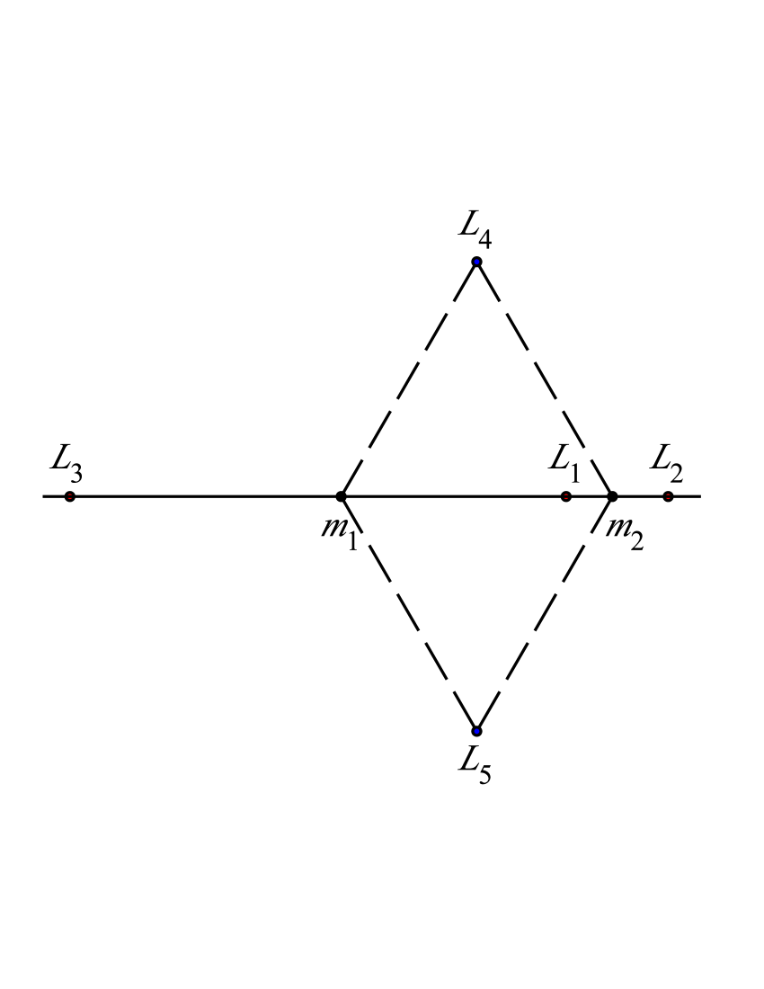
Figure 3.1: Lagrange points $L_{1}$, $L_{2}$, $\dots$, $L_{5}$ in the three-body problem. Two masses labeled with $m_{1}$ and $m_{2}$ are at the indicated positions. The third body has mass $m_{3}$. The positions of the Lagrange points depend only on the mass ratios between $m_{1}$, $m_{2}$, and $m_{3}$. For this plot masses with $m_{2}/m_{1}=m_{3}/m_{1}=0.1$ were used.

3.5 Planetary ephemerides

Summary: Modern ephemerides: dynamical models, observations, representations.

Modern ephemerides of the solar system bodies are numerical solutions obtained by numerical integration of the differential equations of motion and by fitting the initial conditions of these integrations and other parameters of the force model to observational data.

The equations of motion used here are the $N$-body equations discussed above augmented by a number of smaller forces. These forces include relativistic $N$-body forces (the so-called Einstein-Infeld-Hoffmann equations), Newtonian forces due to asteroids, the effects of the figures (non-sphericity) of the Earth, Moon and the Sun as well as some non-gravitational forces. For the Sun it is sufficient to consider the effect of the second zonal harmonics $J_{2}^{\odot}$. The zonal harmonics $J_{n}$ of the Earth and the Moon are usually used up to $n\leq 4$. Mostly one needs forces coming from the interaction of these zonal harmonics with other bodies modeled as point masses. The dynamics of the Earth-Moon system requires even more detailed modeling since the translational motion of the Earth and the Moon are coupled with their rotational motions and deformations in a tricky way. For the Moon even more subtle effects due to tesseral harmonics $C_{nk}$ and $S_{nk}$ again with $n\leq 4$ should be taken into account. Tidal deformations of the Earth’s gravitational field influence the translational motion of the Moon and should be taken into account. Rotational motion of the Earth is well known and obtained from dedicated observations by the International Earth Rotation and Reference Systems Service (IERS). These results are good enough and usually taken for granted for the solar system ephemerides. Rotational motion of the Moon is often called physical libration and is an important part of the process of construction of solar system ephemerides. Physical libration is modeled as rotational motion of a solid body with tidal and rotational distortions, including both elastic and dissipational effects. A discussion of all these forces coming from the non-point-like structure of gravitating bodies can be found in Standish & Williams (2010).

Asteroids play an important role for high-accuracy modeling of the motion of the inner solar system, the motion of Mars being especially sensitive to the quality of the model of asteroids. Since masses of asteroids are poorly known for most of them, the modeling is not trivial. Usually, asteroids are treated in three different ways. A number of “big” asteroids are integrated together with the major planets, the Moon and the Sun. For these “big” asteroids the masses are estimated from the same observational data that are used to fit the ephemeris. Among these “big” asteroids are always “the big three” – Ceres, Pallas and Vesta – and, sometimes, up to several ten asteroids which influence the motion of Mars more than other asteroids. For some hundred asteroids their masses are estimated using their taxonomic (spectroscopic) classes and their estimated radii that are determined by photometry, radar data or observations of stellar occultations by asteroids. For each of the three taxonomic classes Ð C (carbonaceous chondrite), S (stony) and M (iron) Ð the mean density is determined as a part of the ephemeris construction. The cumulative effect of other asteroids is sometimes empirically modeled by a homogeneous massive ring in the plane of ecliptic. The mass of the ring and its radius are again estimated from the same data that are used for the ephemeris (Pitjeva, 2007; Kuchynka et al. 2010).

Since the equations of motion are ordinary differential equations any method for numerical integration of ordinary differential equations can be used to solve them. A very good practical overview of numerical integration methods is given in Chapter 4 of Montenbruck & Gill (2000). Even more details can be found in Chapter 7 of Beutler (2005, Part I). In practice, for planetary motion, one uses either multistep Adams (predictor-corrector) methods (Standish & Williams, 2008; Fienga et al., 2008) or the Everhart integrator (Everhart, 1985; Pitjeva, 2005). The latter is a special sort of implicit Runge-Kutta integrators. Numerical round-off errors are an important issue for the integrations of planetary ephemerides. Usual double precision (64 bit) arithmetic is not sufficient to achieve the goal accuracy and one often uses quadruple precision (128 bit) arithmetic. Since the beginning of the 1970s the JPL ephemeris team uses the variable stepsize, variable order multistep Adams integrators called DIVA/QIVA (Krogh, 2004). Fienga at al. (2008) have shown that only a few arithmetical operations in the classical Adams integrator of order 12 must be performed with quadruple precision to achieve an acceptable accuracy over longer integration intervals. This substantially increases the performance of numerical integrations.

Observational data used for planetary ephemerides include radar observations of earth-like planets, radar and Doppler observations of spacecrafts (especially planetary orbiters), VLBI observations of spacecrafts relative to some reference quasars, Lunar Laser Ranging data, and, finally, optical positional observations of major planets and their satellites (especially important for outer planets with very few radiometric observations).

A total of 250 parameters are routinely fitted for the construction of planetary ephemerides. These parameters include initial positions and velocities of the planets and some of their satellites, the orientation of the frame with respect to the ICRF, the value of Astronomical Unit in meters (or the mass parameter $GM_{\odot}$ of the Sun), the parameters of the model for asteroids (see above), various parameters describing rotational and translational motion of the Earth-Moon system, various parameters used in the reduction of observational data (phase corrections for planetary disk observations, corrections to precession and equinox drift, locations of various relevant sites on the Earth and other bodies, parameters of the solar corona, parameters describing the geometrical figures of Mercury, Venus and Mars, etc.). Useful discussion of various models used for data modeling is given by Moyer (2003) and Standish & Williams (2010). The masses of the major planets can be also fitted from the same data, but, when available, they are taken from the special solutions for the data of planetary orbiters. However, the masses of the Earth and the Moon are often determined in the process of construction of planetary ephemerides.

Modern ephemerides are represented in the form of Chebyshev polynomials. The details of the representation can vary from one ephemeris to another, but the principles are the same: each scalar quantity is represented by a set of polynomials $p_{i}$ of the form

$$p_{i}(t)=\sum_{k=0}^{N_{i}}a_{k}^{(i)}T_{k}(x),\quad x={2t-t_{i}-t_{i+1}\over t_{i+1}-t_{i}},$$ (3.16)

where $T_{k}(x)$ are the Chebyshev polynomials of the first kind (given by the recurrent relations $T_{0}=1$, $T_{1}=x$, and $T_{k+1}=2xT_{k}-T_{k-1}$), and coefficients $a_{k}^{(i)}$ are real numbers. Each polynomial $p_{i}(t)$ is valid for some interval of time $t_{i}\leq t\leq t_{i+1}$ (so that $-1\leq x\leq 1$). The representation (3.16) is close to the optimal uniform approximation of a function by polynomials of given order (Press et al., 2007, Section 5.8), and, thus, gives nearly optimal representation of a function using given number of free parameters. The orders of polynomials $N_{i}$ are usually the same for all time intervals, but do depend on the quantity to be represented. Sometimes (e.g. for the JPL ephemerides) one polynomial represents both the position and the velocity of a body. The velocity can be then calculated as a derivative of (3.16):

$${d\over dt}\,p_{i}(t)={2\over t_{i+1}-t_{i}}\sum_{k=1}^{N_{i}}ka_{k}^{(i)}U_{k}(x),$$ (3.17)

where $U_{k}$ are the Chebyshev polynomials of the second kind (given by the recurrent relations $U_{0}=1$, $U_{1}=2x$, and $U_{k+1}=2xU_{k}-U_{k-1}$). At the boundaries $t_{i}$ of the time intervals, the polynomials $p_{i}$ must satisfy conditions like $p_{i-1}(t_{i})=p_{i}(t_{i})$, so that the approximating function is continuous. One can also imply additional constraints ${d\over dt}\,p_{i-1}(t_{i})={d\over dt}\,p_{i}(t_{i})$ for the derivatives to make the approximating function continuously differentiable. An efficient technique to compute the coefficients $a_{k}^{(i)}$ starting from values of the quantity to be represented is described by Newhall (1989).

There are three sources of modern planetary ephemerides: Jet Propulsion Laboratory (JPL, Pasadena, USA; DE ephemerides), Institut de Méchanique Céleste et de Calcul des Éphémérides (IMCCE, Paris Observatory, France; INPOP ephemerides) and Institute of Applied Astronomy (IAA, St.Petersburg, Russia; EPM ephemerides). All of them are available from the Internet:

• http://ssd.jpl.nasa.gov/?planet_eph_export for the DE ephemerides,

• http://www.imcce.fr/fr/presentation/equipes/ASD/inpop/ for the INPOP, and

• ftp://quasar.ipa.nw.ru/incoming/EPM2004/ for the EPM ephemerides.

Different versions of the ephemerides have different intervals of validity, but typically these are several hundred years around the year 2000. Longest readily available ephemerides are valid for a time span of 6000 years. Further details on these ephemerides can be found in Standish & Williams (2010), Folkner (2010), Fienga et al. (2008), and Pitjeva (2005), respectively.

Let us also mention that for the lower-accuracy applications, semi-analytical theories of planetary motion called VSOP are available (Bretagnon, Francou, 1988; Moisson, Bretagnon, 2001). The semi-analytical theories are given in the form of Poisson series $\sum_{k}c_{k}t^{n_{k}}\cos(a_{k}t+b_{k})$, where $a_{k}$, $b_{k}$, and $c_{k}$ are real numbers, and $n_{k}$ is the integer power of time $t$. Formally any value of time can be substituted into such series, but the theory is meaningful only for several thousand years around the year 2000. The VSOP ephemeris contains only major planets and the Earth-Moon barycenter. The best semi-analytical theory of motion of the Moon with respect to the Earth is called ELP82. This theory can also be used in low-accuracy applications.

Chapter 4 Elements of the Perturbation Theory

4.1 The method of the variation of constants

Summary: The variation of constants as a method to solve differential equations. Instantaneous elements. Osculating elements.

The equations of motion of two-body problem considered above in great detail read

$$\ddot{{\mbox{\boldmath$r$}}}+\kappa^{2}\,{{\mbox{\boldmath$r$}}\over r^{3}}=0.$$

The simplicity of the two-body motion and the fact that many practical problems of celestial mechanics are sufficiently close to two-body motion make it practical to use two-body motion as zero approximation to the motion in more realistic cases and treat the difference by the usual perturbative approach. Special technique for the motion of celestial bodies is called osculating elements. The solution of the two-body problem discussed above can be symbolically written as

$${\mbox{\boldmath$r$}}={\mbox{\boldmath$f$}}(t,e_{1},e_{2},e_{3},e_{4},e_{5},e_{6}),\qquad e_{i}={\rm const},\ i=1\dots 6,$$ (4.1)

where $e_{i}$ are six Keplerian elements: semi-major axis $a$, eccentricity $e$, inclination $i$, argument of pericenter $\omega$ and longitude of the node $\Omega$. In general case of arbitrary additional forces it is always possible to write the equations of motion of a body as

$$\ddot{{\mbox{\boldmath$r$}}}+\kappa^{2}\,{{\mbox{\boldmath$r$}}\over r^{3}}={\mbox{\boldmath$F$}},$$ (4.2)

where ${\mbox{\boldmath$F$}}={\mbox{\boldmath$F$}}(t,{\mbox{\boldmath$r$}},\dot{{\mbox{\boldmath$r$}}},\dots)$ is arbitrary force depending in general on the position and velocity of the body under study, time and any other parameters. One example of such a disturbing force is given by (3.13) for the $N$-body problem. The general idea is to use the same functional form for the solution of (4.2) as we had for the two-body motion, but with constants (former Kepler elements) being time-dependent:

$${\mbox{\boldmath$r$}}={\mbox{\boldmath$f$}}(t,e_{1},e_{2},e_{3},e_{4},e_{5},e_{6}),\qquad e_{i}=e_{i}(t),\ i=1\dots 6.$$ (4.3)

This is always possible since $F$ has three degrees of freedom (three arbitrary components) and representation (4.3) involves six arbitrary functions of time. Let us stress the following. Eq. (4.3) means that if elements $e_{i}(t)$ are given for some $t$, the position $r$ of the body under study for that $t$ can be computed using usual formulas of two-body problem as summarized in Section 2.8. The idea of (4.3) is closely related to the idea of the method of variation of constants, also known as variation of parameters, developed by Joseph Louis Lagrange. This method is a general method to solve inhomogeneous linear ordinary differential equations.

As mentioned above the representation in (4.3) has three “redundant” degrees of freedom. These three degrees of freedom can be used to make it possible to compute not only position $r$, but also velocity $\dot{{\mbox{\boldmath$r$}}}$ from the solution of (4.2) using standard formulas of the two-body problem summarized in Section 2.8. This can be done if the elements $e_{i}(t)$ satisfy the following condition

$$\sum_{i=1}^{6}{\partial{\mbox{\boldmath$f$}}\over\partial e_{i}}\,\dot{e}_{i}=0\,.$$ (4.4)

Indeed, in general case, time derivative of $r$ given by (4.3) reads

$$\dot{{\mbox{\boldmath$r$}}}={\partial{\mbox{\boldmath$f$}}\over\partial t}+\sum_{i=1}^{6}{\partial{\mbox{\boldmath$f$}}\over\partial e_{i}}\,\dot{e}_{i}\,.$$ (4.5)

Therefore, condition (4.4) guarantees that the time derivative of (4.3) is given by the partial derivative of $f$ with respect to time

$$\dot{{\mbox{\boldmath$r$}}} = {\partial\over\partial t}\,{\mbox{\boldmath$f$}}(t,e_{1},e_{2},e_{3},e_{4},e_{5},e_{6})\,.$$ (4.6)

This means that velocity $\dot{{\mbox{\boldmath$r$}}}$ can be calculated by the standard formulas of two-body problem (indeed, (4.6) coincided with the derivative of (4.1 with constant $e_{i}$ that represent the usual solution of the two-body problem). The elements having these properties are called osculating elements. The osculating elements are in general functions of time. To compute position and velocity at any given moment one first has to calculate the values of the six osculating elements for this moment of time and then use the standard equations summarized in Section 2.8.

Let us stress that, with osculating elements, not only vectors of position $r$ and velocity $\dot{{\mbox{\boldmath$r$}}}$ can be computed using formulas of the two-body problem, but also any functions of these two vectors. Let us give an explicit example here. For a given moment of time $t$ the absolute value of $r$ is given as $r(t)=a(t)\,(1-e(t)\,\cos E(t))$. Here $a(t)$ and $e(t)$ are osculating semi-major axes and eccentricity. Osculating eccentric anomaly $E(t)$ can be computed from Kepler equation $E-e(t)\sin E=M$, where again osculating eccentricity $e(t)$ should be used. The derivative of $r$ can be computed $\dot{r}=\dot{E}\,a\,e\,\cos E=a\,e\,\cos E\,{\kappa\,a^{-3/2}\over 1-e\,\cos E}={\kappa\,e\over\sqrt{a\,(1-e^{2})}}\,\sin v$ and all elements are again functions of time: $a=a(t)$, $e=e(t)$, etc. Also the anomalies – eccentric $E$, true $v$ and mean $M$ – are related to each other in the same way as in the two-body problem.

4.2 Gaussian perturbation equations

Summary: The radial, tangential and transverse components of the disturbing force. The Gaussian perturbation equations: the differential equations for the osculating elements. Other variants of the Gaussian perturbation equations.

Let us derive the equations for osculating elements for a general disturbing force $F$. First, we introduce a new Cartesian coordinate system. The origin of the new system $(S,T,W)$ is the same as usual, but the orientation is different and depends at each moment of time on the position $r$ and velocity $\dot{{\mbox{\boldmath$r$}}}$ of the considered body. Axis $S$ is directed radially, that is parallel to $r$. Axis $T$ lies in the momentary orbital plane (the plane containing both $r$ and $\dot{{\mbox{\boldmath$r$}}}$), perpendicular to $S$ (and, therefore, to $r$) and the angle between $T$ and $\dot{{\mbox{\boldmath$r$}}}$ does not exceed $90^{\circ}$. Axis $W$ is perpendicular to both $S$ and $T$ (that is, perpendicular to both $r$ and $\dot{{\mbox{\boldmath$r$}}}$) and completes $S$ and $T$ to a right-hand coordinate system $(S,T,W)$. Coordinates $(S,T,W)$ rotate as the body moves along its orbit.

The components of disturbing force $F$ in axes $(S,T,W)$ are also denoted by $(S,T,W)$ and can be computed as

$$S = {{\mbox{\boldmath$r$}}\over r}\cdot{\mbox{\boldmath$F$}},$$ (4.7)

$$T = {\left({\mbox{\boldmath$r$}}\times\dot{{\mbox{\boldmath$r$}}}\right)\times{\mbox{\boldmath$r$}}\over\left|{\mbox{\boldmath$r$}}\times\dot{{\mbox{\boldmath$r$}}}\right|\,r}\cdot{\mbox{\boldmath$F$}},$$ (4.8)

$$W = {{\mbox{\boldmath$r$}}\times\dot{{\mbox{\boldmath$r$}}}\over\left|{\mbox{\boldmath$r$}}\times\dot{{\mbox{\boldmath$r$}}}\right|}\cdot{\mbox{\boldmath$F$}},$$ (4.9)

where ’$\cdot$’ and ’$\times$’ denote the scalar and cross products of two vectors. Obviously, the relation of $(S,T,W)$ and our usual coordinates $(x,y,z)$ reads

$$\pmatrix{a_{x}\cr a_{y}\cr a_{z}}={\hbox{\bf A}}^{T}_{z}(\Omega)\,{\hbox{\bf A}}^{T}_{x}(i)\,{\hbox{\bf A}}^{T}_{z}(u)\,\pmatrix{a_{A}\cr a_{T}\cr a_{W}},$$ (4.10)

where angle $u=v+\omega$ is called argument of latitude. The matrix ${\hbox{\bf A}}^{T}_{z}(\Omega)\,{\hbox{\bf A}}^{T}_{x}(i)\,{\hbox{\bf A}}^{T}_{z}(u)$ is given by (2.33) with $u$ substituted for $\omega$. Here for an arbitrary vector $a$ its components in coordinates $(x,y,z)$ are denoted as $(a_{x},a_{y},a_{z})$ and the corresponding components in coordinates $(S,T,W)$ are $(a_{S},a_{T},a_{W})$.

4.2.1 Derivation of differential equations for osculating elements

Now, let us derive the required equations one by one. First, let us consider the integral of areas ${\mbox{\boldmath$c$}}={\mbox{\boldmath$r$}}\times\dot{{\mbox{\boldmath$r$}}}$. This leads to $c^{2}=({\mbox{\boldmath$r$}}\times\dot{{\mbox{\boldmath$r$}}})\,\cdot\,({\mbox{\boldmath$r$}}\times\dot{{\mbox{\boldmath$r$}}})$, where $c=|{\mbox{\boldmath$c$}}|$. A time derivative of $c^{2}$ then reads

$${dc^{2}\over dt}=2\,({\mbox{\boldmath$r$}}\times\dot{{\mbox{\boldmath$r$}}})\,\cdot\,({\mbox{\boldmath$r$}}\times\ddot{{\mbox{\boldmath$r$}}})=2\,({\mbox{\boldmath$r$}}\times\dot{{\mbox{\boldmath$r$}}})\,\cdot\,({\mbox{\boldmath$r$}}\times{\mbox{\boldmath$F$}})=2\left(\left({\mbox{\boldmath$r$}}\times\dot{{\mbox{\boldmath$r$}}}\right)\times{\mbox{\boldmath$r$}}\right)\cdot{\mbox{\boldmath$F$}}=2\,r^{2}\,\dot{{\mbox{\boldmath$r$}}}\cdot{\mbox{\boldmath$F$}}-2\,r\,\dot{r}\,{\mbox{\boldmath$r$}}\cdot{\mbox{\boldmath$F$}}$$

($\dot{{\mbox{\boldmath$r$}}}\cdot{\mbox{\boldmath$r$}}=\dot{r}\,r$ is used here). Since ${\mbox{\boldmath$F$}}=(S,T,W)$ and ${\mbox{\boldmath$r$}}=(r,0,0)$ in STW-coordinates one gets ${\mbox{\boldmath$r$}}\cdot{\mbox{\boldmath$F$}}=r\,S$. Let us now consider $\dot{{\mbox{\boldmath$r$}}}\cdot{\mbox{\boldmath$F$}}$. We need vectors $\dot{{\mbox{\boldmath$r$}}}$ and $F$ in STW-coordinates. Since the instantaneous plane of the orbit is defined by the instantaneous position and velocity vectors of the body, the $W$ component of the velocity $\dot{{\mbox{\boldmath$r$}}}$ vanish by definition. Obviously, the $S$ component is $\dot{r}$ and the T component is $r\dot{v}$. For the latter from the integral of areas in polar coordinates $r^{2}\,\dot{v}=\kappa\,\sqrt{p}$, one has $r\dot{v}={\kappa\,\sqrt{p}\over r}$. Therefore, in STW coordinates $\dot{{\mbox{\boldmath$r$}}}=(\dot{r},{\kappa\,\sqrt{p}\over r},0)$. Therefore, $\dot{{\mbox{\boldmath$r$}}}\cdot{\mbox{\boldmath$F$}}=\dot{r}\,S+{\kappa\,\sqrt{p}\over r}\,T$. Substituting ${\mbox{\boldmath$r$}}\cdot{\mbox{\boldmath$F$}}$ and $\dot{{\mbox{\boldmath$r$}}}\cdot{\mbox{\boldmath$F$}}$ into the equation for ${dc^{2}\over dt}$ derived above and taking into account that the semi-latus rectum $p=c^{2}/\kappa^{2}$ we get

$$\dot{p}=2\,p\,r\,\left({T\over\kappa\,\sqrt{p}}\right).$$ (4.11)

Now, let us consider the time derivative of the integral of area itself. One has ${\mbox{\boldmath$c$}}={\mbox{\boldmath$r$}}\times\dot{{\mbox{\boldmath$r$}}}$ and, therefore, $\dot{{\mbox{\boldmath$c$}}}={d\over dt}\,\left({\mbox{\boldmath$r$}}\times\dot{{\mbox{\boldmath$r$}}}\right)={\mbox{\boldmath$r$}}\times\ddot{{\mbox{\boldmath$r$}}}={\mbox{\boldmath$r$}}\times{\mbox{\boldmath$F$}}$. It is clear that $c$ is parallel to axis W of the STW system (since $c$ is defined as ${\mbox{\boldmath$c$}}={\mbox{\boldmath$r$}}\times\dot{{\mbox{\boldmath$r$}}}$ it is perpendicular to both $r$ and $\dot{{\mbox{\boldmath$r$}}}$). For this reasons and considering that $c=\kappa\,\sqrt{p}$, the components of $c$ in STW axes read ${\mbox{\boldmath$c$}}=(0,0,\kappa\,\sqrt{p})$. Using transformation (4.10) to convert the $STW$-components into $xyz$-ones, one gets

$$\pmatrix{c_{x}\cr c_{y}\cr c_{z}}=\left(\begin{array}[]{r}\sin i\,\sin\Omega\,\kappa\,\sqrt{p}\\ -\sin i\,\cos\Omega\,\kappa\,\sqrt{p}\\ \cos i\,\kappa\,\sqrt{p}\end{array}\right)\,.$$ (4.12)

In the STW system one has ${\mbox{\boldmath$r$}}=(r,0,0)$ and ${\mbox{\boldmath$F$}}=(S,T,W)$. Therefore, in STW components one gets ${\mbox{\boldmath$r$}}\times{\mbox{\boldmath$F$}}=(0,-r\,W,r\,T)$. Again using transformation (4.10) it is easy to calculate that the z component of ${\mbox{\boldmath$r$}}\times{\mbox{\boldmath$F$}}$ reads $\left({\mbox{\boldmath$r$}}\times{\mbox{\boldmath$F$}}\right)_{z}=-\sin i\,\cos u\,r\,W+\cos i\,r\,T$. Considering the z component of $\dot{{\mbox{\boldmath$c$}}}={\mbox{\boldmath$r$}}\times{\mbox{\boldmath$F$}}$ one gets

$${d\over dt}\,c_{z}=-\sin i\,\cos u\,r\,W+\cos i\,r\,T\,.$$

On the other hand, from (4.12) one gets

$${d\over dt}\,c_{z}={d\over dt}\,\left(\cos i\,\kappa\,\sqrt{p}\right)=-\kappa\,\sqrt{p}\,\sin i{d\over dt}\,i+\cos i\,{d\over dt}\,\left(\kappa\,\sqrt{p}\right)\,.$$

From (4.11) it is easy to see that

$${d\over dt}\,\left(\kappa\,\sqrt{p}\right)=\kappa\,{1\over 2\,\sqrt{p}}\ \dot{p}=r\,T\,,$$

and we finally get the following equation for the derivative of inclination $i$:

$${d\over dt}\,i=r\,\cos u\,\left({W\over\kappa\,\sqrt{p}}\right)\,.$$ (4.13)

Analogously, considering the time derivative of $c_{x}=\sin i\sin\Omega\,\kappa\,\sqrt{p}$ and computing the x component of ${\mbox{\boldmath$r$}}\times{\mbox{\boldmath$F$}}$ from (4.10) one gets

$${d\over dt}\,c_{x}={d\over dt}\,\left(\sin i\,\sin\Omega\,\kappa\,\sqrt{p}\right)=(-\cos\Omega\,\sin u-\cos i\,\sin\Omega\,\cos u)\,(-r\,W)+\sin i\,\sin\Omega\,r\,T\,.$$

Using here equations (4.11) and (4.13) for $\dot{p}$ and ${d\over dt}\,i$ one gets the equation for the time derivative of $\Omega$:

$${d\over dt}\,\Omega={r\,\sin(v+\omega)\over\sin i}\,\left({W\over\kappa\sqrt{p}}\right)\,.$$ (4.14)

Clearly, the y component of $\dot{{\mbox{\boldmath$c$}}}=\left({\mbox{\boldmath$r$}}\times{\mbox{\boldmath$F$}}\right)$ gives no new information since $c_{y}$ depends on the same elements as $c_{x}$. We have therefore got all possible equations from the integral of areas of the two-body problem. Now let us turn to the integral of energy (2.12). This integral can be rewritten in the form

$${1\over 2}\,\dot{{\mbox{\boldmath$r$}}}\cdot\dot{{\mbox{\boldmath$r$}}}-{\kappa^{2}\over r}=-{\kappa^{2}\over 2a}.$$ (4.15)

The derivative of this equation

$$\dot{{\mbox{\boldmath$r$}}}\cdot\ddot{{\mbox{\boldmath$r$}}}+{\kappa^{2}\over r^{2}}\,\dot{r}={\kappa^{2}\over 2a^{2}}\,\dot{a}$$

can be simplified using

$$\dot{{\mbox{\boldmath$r$}}}\cdot\ddot{{\mbox{\boldmath$r$}}}=\dot{{\mbox{\boldmath$r$}}}\cdot\left(-{\kappa^{2}\over r^{3}}\,{\mbox{\boldmath$r$}}+{\mbox{\boldmath$F$}}\right)=-{\kappa^{2}\over r^{3}}\,\dot{{\mbox{\boldmath$r$}}}\cdot{\mbox{\boldmath$r$}}+\dot{{\mbox{\boldmath$r$}}}\cdot{\mbox{\boldmath$F$}},$$

$$\dot{{\mbox{\boldmath$r$}}}\cdot\ddot{{\mbox{\boldmath$r$}}}+{\kappa^{2}\over r^{2}}\,\dot{r}=-{\kappa^{2}\over r^{3}}\,\dot{{\mbox{\boldmath$r$}}}\cdot{\mbox{\boldmath$r$}}+\dot{{\mbox{\boldmath$r$}}}\cdot{\mbox{\boldmath$F$}}+{\kappa^{2}\over r^{2}}\,\dot{r}=\dot{{\mbox{\boldmath$r$}}}\cdot{\mbox{\boldmath$F$}}$$

(here we used that $\dot{r}\,r=\dot{{\mbox{\boldmath$r$}}}\cdot{\mbox{\boldmath$r$}}$) and computing $\dot{{\mbox{\boldmath$r$}}}\cdot{\mbox{\boldmath$F$}}$ from the STW components of $\dot{{\mbox{\boldmath$r$}}}$ and $F$ already given above

$$\dot{{\mbox{\boldmath$r$}}}\cdot{\mbox{\boldmath$F$}}=\dot{r}\,S+{\kappa\,\sqrt{p}\over r}\,T\,.$$

This allows one to get the equation for $\dot{a}$:

$${d\over dt}\,a=2\,a^{2}\,e\,\sin v\,\left({S\over\kappa\sqrt{p}}\right)+2\,a^{2}\,{p\over r}\,\left({T\over\kappa\sqrt{p}}\right)\,.$$ (4.16)

Here we used that $\dot{r}={\kappa e\over\sqrt{p}}\,\sin v$. Having equations (4.11) and (4.16) for $\dot{p}$ and $\dot{a}$ it is easy to derive the equation for $\dot{e}$. Indeed, from $p=a(1-e^{2})$ one gets $\dot{p}=\dot{a}(1-e^{2})-2e\,a\,\dot{e}$. Solving for $\dot{e}$ and substituting (4.11) and (4.16) one gets

$${d\over dt}\,e=p\,\sin v\,\left({S\over\kappa\sqrt{p}}\right)+p\,(\cos v+\cos E)\,\left({T\over\kappa\sqrt{p}}\right)\,.$$ (4.17)

Now, let us turn to the derivation of $\dot{\omega}$. The derivation consists of several steps. First, from

$$r={p\over 1+e\cos v}$$

one gets

$$1+e\,\cos v={p\over r}.$$

Computing time derivative of the latter equations

$$-e\,\sin v\,\dot{v}+\dot{e}\,\cos v={\dot{p}\over r}-{p\over r^{2}}\,\dot{r}$$

and using equations for $\dot{r}$, $\dot{p}$ and $\dot{e}$ derived above one gets the derivative of true anomaly $v$ as

$$\dot{v}={\kappa\,\sqrt{p}\over r^{2}}+{p\,\cos v\over e}\,\left({S\over\kappa\,\sqrt{p}}\right)-{p+r\over e}\,\sin v\,\left({T\over\kappa\,\sqrt{p}}\right)\,.$$ (4.18)

As the second step in the derivation of $\dot{\omega}$, let us consider the formula for the z component of vector $r$: $z=r\,\sin i\,\sin u$, where $u=v+\omega$. This formula can be derived e.g., from the equation immediately before (3). On the one hand, $\dot{z}$ is the component of the velocity vector $\dot{{\mbox{\boldmath$r$}}}$ and can be calculated considering all osculating elements as constants (from the integral of area in polar coordinates $r^{2}\,\dot{v}=\kappa\,\sqrt{p}$ one has $\dot{v}={\kappa\,\sqrt{p}\over r^{2}}$):

$$\dot{z}=\dot{r}\,\sin i\,\sin u+r\,\dot{v}\,\sin i\,\cos u=\dot{r}\,\sin i\,\sin u+r\,{\kappa\sqrt{p}\over r^{2}}\sin i\,\cos u$$

However, the same $\dot{z}$ can be computed not assuming that the osculating elements are constants (that is, explicitly considering the time derivatives of the osculating elements). This should give the same results according to the idea of osculating elements described in Section 4.1. Therefore, one has

$$\dot{z}=\dot{r}\,\sin i\,\sin u+r\,\cos i\,\sin u\,{di\over dt}+r\,\sin i\,\cos u\,{du\over dt}\,.$$

Equating the last two expressions for $\dot{z}$ one gets

$$\dot{u}={\kappa\sqrt{p}\over r^{2}}-\cot i\,\tan u\,{di\over dt}.$$ (4.19)

Finally, since $u=v+\omega$ one has $\dot{\omega}=\dot{u}-\dot{v}$ and using equations (4.19) and (4.18) for $\dot{u}$ and $\dot{v}$ and (4.13) for ${di\over dt}$ one gets

$${d\over dt}\,\omega=-{p\,\cos v\over e}\,\left({S\over\kappa\sqrt{p}}\right)+{r+p\over e}\,\sin v\,\left({T\over\kappa\sqrt{p}}\right)-r\,\sin(v+\omega)\,\cot i\,\left({W\over\kappa\sqrt{p}}\right)\,.$$ (4.20)

The only equation still to be derived is that for the mean anomaly of an epoch. Let us first consider the definition of the mean anomaly

$$M=M_{0}+n(t-t_{0})\,,$$ (4.21)

where $t_{0}$ is a given fixed epoch for which $M=M_{0}$. In the framework of the two-body problem $n=\kappa\,a^{-3/2}$ is constant. In case of osculating elements $n$ is time-dependent (since $a$ is time-dependent) and the derivative of $M$ reads

$${d\over dt}\,M={d\over dt}\,M_{0}+n+{dn\over dt}\,(t-t_{0}).$$ (4.22)

This formula contains time $t$ explicitly. This is not convenient for many applications. This can be avoided if instead of (4.21) one defines the mean anomaly as

$$M=\overline{M}_{0}+\int_{t_{0}}^{t}n\,dt\,.$$ (4.23)

In the framework of the two-body problem (4.23) is fully equivalent to (4.21). However, for osculating elements derivative of $M$ from (4.23) reads

$${d\over dt}\,M={d\over dt}\,\overline{M}_{0}+n\,.$$ (4.24)

Clearly, ${d\over dt}\,\overline{M}_{0}={d\over dt}\,M_{0}+\dot{n}\,(t-t_{0})$, where $\dot{n}={dn\over dt}=-{3\over 2}\,\kappa\,a^{-5/2}\,\dot{a}$. Definition (4.23) is used below.

In order to derive the equation for ${d\over dt}\,\overline{M}_{0}$ let us consider two equations

$$E-e\,\sin E=M\,,$$

$$r=a\,(1-e\,\cos E)\,.$$

Differentiating these equations one gets

$$\dot{E}\,(1-e\,\cos E)-\dot{e}\,\sin E=\dot{M},$$

$$\dot{r}=\dot{a}\,(1-e\,\cos E)-a\,\dot{e}\,\cos E+a\,e\,\sin E\,\dot{E}.$$

Considering that $\dot{r}={\kappa\over\sqrt{p}}\,e\,\sin v$ one gets

$$\dot{M}=n+{\sqrt{1-e^{2}}\over e}\,\left(\dot{e}\,\cot v-\dot{a}\,{r\over a^{2}\,\sin v}\right)\,.$$ (4.25)

Comparing to (4.24) and substituting (4.17) and (4.16) for $\dot{e}$ and $\dot{a}$ one finally gets

$${d\over dt}\,\overline{M}_{0}={\sqrt{1-e^{2}}\over e}\,\left(\left(p\cos v-2\,e\,r\right)\,\left({S\over\kappa\sqrt{p}}\right)-(r+p)\sin v\,\left({T\over\kappa\sqrt{p}}\right)\right).$$ (4.26)

4.2.2 Discussion of the derived equations

Gathering all equations for the derivatives of osculating elements derived above one gets the full set of equations:

$${d\over dt}\,a = 2\,a^{2}\,e\,\sin v\,\left({S\over\kappa\sqrt{p}}\right)+2\,a^{2}\,{p\over r}\,\left({T\over\kappa\sqrt{p}}\right),$$ (4.27)

$${d\over dt}\,e = p\,\sin v\,\left({S\over\kappa\sqrt{p}}\right)+p\,(\cos v+\cos E)\,\left({T\over\kappa\sqrt{p}}\right),$$ (4.28)

$${d\over dt}\,i = r\,\cos(v+\omega)\,\left({W\over\kappa\sqrt{p}}\right),$$ (4.29)

$${d\over dt}\,\omega = -{p\,\cos v\over e}\,\left({S\over\kappa\sqrt{p}}\right)+{r+p\over e}\,\sin v\,\left({T\over\kappa\sqrt{p}}\right)-r\,\sin(v+\omega)\,\cot i\,\left({W\over\kappa\sqrt{p}}\right),$$ (4.30)

$${d\over dt}\,\Omega = {r\,\sin(v+\omega)\over\sin i}\,\left({W\over\kappa\sqrt{p}}\right),$$ (4.31)

$${d\over dt}\,\overline{M}_{0} = {\sqrt{1-e^{2}}\over e}\,\left(\left(p\cos v-2\,e\,r\right)\,\left({S\over\kappa\sqrt{p}}\right)-(r+p)\sin v\,\left({T\over\kappa\sqrt{p}}\right)\right).$$ (4.32)

These equations were derived by Johann Carl Friedrich Gauß (1777 – 1855) and called Gaussian perturbation equations. The equations were also independently derived by Leonhard Euler some time before Gauss and are sometimes called Euler equations. We will use these equations below when discussing the influence of atmospheric drag on the motion of Earth’s satellites.

Numerous alternative forms of the Gaussian perturbation equations are given in Beutler (2005). In particular, one can use any other components of the disturbing force $F$ instead of $(S,T,W)$. Eqs. (4.27)–(4.32) are valid for elliptic motion ($e<1$). Similar equations for hyperbolic motion with $e>1$ can be derived, but are rarely used in practice. Let us note that Eqs. (4.27)–(4.32) have singularities for $e=0$ or very small $e$ (equations for $\omega$ and $\overline{M}_{0}$), $i=0$ and $i=\pi$ (equations for $\omega$ and $\Omega$), and $e$ close to 1 (e.g. since $p$ is small for this case). Indeed, the right-hand sides of the equations are not well defined in these cases. These singularities are related to the fact that some of the Keplerian elements are not well defined for $e=0$, $i=0$ or $i=\pi$. If the application requires these cases to be included one introduces

$$h = e\,\sin\omega,$$

$$k = e\,\cos\omega,$$ (4.33)

instead of $e$ and $\omega$ and

$$p = \tan i\,\sin\Omega,$$

$$q = \tan i\,\cos\Omega.$$ (4.34)

instead of $i$ and $\Omega$. The equations for the derivatives $h$, $k$, $p$ and $q$ can be easily derived from (4.27)–(4.32). The equations for $\dot{h}$, $\dot{k}$, $\dot{p}$ and $\dot{q}$ and do not contain singularities.

Exercise. Derive equations for the derivatives of osculating $h$, $k$, $p$ and $q$ using corresponding equations for $\dot{\omega}$, $\dot{e}$, $\dot{i}$ and $\dot{\Omega}$ in (4.27)–(4.32).

4.3 Lagrange equations

Summary: The potential disturbing force. Lagrange equations for the osculating elements. Properties of the Lagrange equations.

The Gaussian perturbation equations are valid for any disturbing force $F$. For the special case when the perturbing force has a potential $R$ one has

$$F^{i}={\partial\over\partial r^{i}}\,R\,.$$

In this case one can modify the Gaussian perturbation equations so that the disturbing potential $R$ appear in the equations instead of the components of perturbing force $F$. This case of potential perturbations is very important for practical applications. For example, above we have seen that the N-body problem can be considered as perturbed two-body problem with disturbing force having potential (3.15).

In general both $F$ and $R$ can depend on time $t$, position $r$ and velocity $\dot{{\mbox{\boldmath$r$}}}$ of the body under study: $R=R(t,{\mbox{\boldmath$r$}},\dot{{\mbox{\boldmath$r$}}})$. Here we consider the simpler situation when both $F$ and $R$ do not depend of velocity $\dot{{\mbox{\boldmath$r$}}}$. Therefore, we assume that $R=R(t,{\mbox{\boldmath$r$}})$. This covers the most important applications of potential perturbations.

First, we consider potential $R$ as function of osculating elements $R=R(t,e_{1},e_{2},e_{3},e_{4},e_{5},e_{6})$. This parametrization can be directly derived by substituting (4.3) into $R(t,{\mbox{\boldmath$r$}})$. Our goals is to replace the components $S$, $T$ and $W$ of the disturbing force in (4.27)–(4.32) by partial derivatives of $R$. First, we should compute ${\partial R\over\partial e_{i}}$ as functions of $S$, $T$ and $W$. One has

$${\partial R\over\partial e_{i}}=\sum_{i=1}^{3}{\partial R\over\partial r^{j}}\,{\partial r^{j}\over\partial e_{i}}=\sum_{i=1}^{3}F^{j}{\partial r^{j}\over\partial e_{i}}.$$

Here $r^{j}$ is the $j$-th component of vector $r$ and $F^{j}$ is the $j$-th component of $F$. Therefore one should only know ${\partial r^{j}\over\partial e_{i}}$ to compute ${\partial R\over\partial e_{i}}$.

Let us consider the example of semi-major axis $a$. According to the formulas of the two-body problem summarized in Section 2.8, radius-vector $r$ is linearly proportional to $a$. Therefore, one has ${\partial r^{j}\over\partial a}={r^{j}\over a}$ and, finally,

$${\partial R\over\partial a}=\sum_{i=1}^{3}F^{j}{\partial r^{j}\over\partial a}={1\over a}\,\sum_{i=1}^{3}F^{j}r^{j}={1\over a}\,{\mbox{\boldmath$F$}}\cdot{\mbox{\boldmath$r$}}={r\over a}\,S.$$ (4.35)

Analogously, one gets

$${\partial R\over\partial e} = a\left(-S\,\cos v+T\,\left(1+{r\over p}\right)\sin v\right)\,,$$ (4.36)

$${\partial R\over\partial i} = r\,W\,\sin\left(v+\omega\right)\,,$$ (4.37)

$${\partial R\over\partial\omega} = r\,T\,,$$ (4.38)

$${\partial R\over\partial\Omega} = r\,T\,\cos i-r\,W\,\sin i\,\cos\left(v+\omega\right)\,,$$ (4.39)

$${\partial R\over\partial\overline{M}_{0}} = {a\over\sqrt{1-e^{2}}}\,\left(e\,S\,\sin v+{p\over r}\,T\right)\,.$$ (4.40)

Now, one should invert (4.35)–(4.40) to get three components $S$, $T$ and $W$ as functions of six partial derivatives ${\partial R\over\partial e_{i}}$. Clearly, this inversion is not unique. In principle, any possible inverse of (4.35)–(4.40) can be inserted to the Gaussian perturbation equations (4.27)–(4.32) and lead to a correct set of equations for osculating elements. However, the resulting equations can be made especially simple if one requires that the coefficients of ${\partial R\over\partial e_{i}}$ in the final equations do not depend on time explicitly (e.g., do not contain radius-vector $r$ and true anomaly $v$). With this requirement the inversion of (4.35)–(4.40) is also unique. Finally, the equations read

$${d\over dt}\,a = {2\over n\,a}\,{\partial R\over\partial\overline{M}_{0}},$$ (4.41)

$${d\over dt}\,e = {1-e^{2}\over e\,n\,a^{2}}\,{\partial R\over\partial\overline{M}_{0}}-{\sqrt{1-e^{2}}\over e\,n\,a^{2}}\,{\partial R\over\partial\omega},$$ (4.42)

$${d\over dt}\,i = {\cot i\over n\,a^{2}\,\sqrt{1-e^{2}}}\,{\partial R\over\partial\omega}-{{\rm cosec}\,i\over n\,a^{2}\,\sqrt{1-e^{2}}}\,{\partial R\over\partial\Omega},$$ (4.43)

$${d\over dt}\,\omega = {\sqrt{1-e^{2}}\over e\,n\,a^{2}}\,{\partial R\over\partial e}-{\cot i\over n\,a^{2}\,\sqrt{1-e^{2}}}\,{\partial R\over\partial i},$$ (4.44)

$${d\over dt}\,\Omega = {{\rm cosec}\,i\over n\,a^{2}\,\sqrt{1-e^{2}}}\,{\partial R\over\partial i},$$ (4.45)

$${d\over dt}\,\overline{M}_{0} = -{2\over n\,a}\,{\partial R\over\partial a}-{1-e^{2}\over e\,n\,a^{2}}\,{\partial R\over\partial e}\,,$$ (4.46)

where the potential $R$ is considered as function of osculating elements and possibly time $t$: $R=R(t,a,e,i,\omega,\Omega,\overline{M}_{0})$. These equation were first derived by Joseph Louis Lagrange (1736 – 1813) and are called Lagrange equations. Clearly, the Lagrange equations are fully equivalent to the Gaussian perturbation equations.

The structure of the Lagrange equations is very interesting. As noted above time appear in (4.41)–(4.46) (if at all) only in $R$. The coefficients the partial derivatives depend only on osculating elements that are constants in the two-body problem. Furthermore, the elements can be divided into two groups: $\alpha_{k}=(a,e,i)$ and $\beta_{k}=(\omega,\Omega,\overline{M}_{0})$, $k=1,2,3$. Then the Lagrange equations can be symbolically written as

$$\dot{\alpha}_{k} = \sum_{l=1}^{3}A_{kl}\,{\partial R\over\partial\beta_{l}}\,,$$

$$\dot{\beta}_{k} = -\sum_{l=1}^{3}A_{lk}\,{\partial R\over\partial\alpha_{l}}\,.$$

This means that

• the derivatives of the elements of one group depend only on the partial derivatives of $R$ with respect to the elements of the other group and

• if the coefficient of $\displaystyle{\partial R\over\partial\beta_{l}}$ in $\dot{\alpha}_{k}$ is $A_{kl}$ then the same coefficient (with minus) appears at $\displaystyle{\partial R\over\partial\alpha_{k}}$ in $\dot{\beta}_{l}$.

The last property should be illustrated. For example, the coefficient of $\displaystyle{\partial R\over\partial\overline{M}_{0}}$ in ${d\over dt}\,e$ is $\displaystyle{1-e^{2}\over e\,n\,a^{2}}$ (see Eq. (4.42)). The same coefficient $\displaystyle{1-e^{2}\over e\,n\,a^{2}}$ (with minus) appears in front of $\displaystyle{\partial R\over\partial e}$ in ${d\over dt}\,\overline{M}_{0}$ (see Eq. (4.46)). The same symmetry holds for all coefficients. Finally, among nine possible $A_{kl}$ four vanish and one has only five different coefficients in (4.41)–(4.46). This structure of the Lagrange equations is used to introduce the so-called canonical elements which will not be considered here.

Osculating elements are very convenient for analytical assessments of the effects of particular perturbations. They are also widely used for practical representations of orbits of asteroids and artificial satellites. Such a representation is especially efficient when the osculating elements can be represented using simple functions of time requiring a limited number of numerical parameters (i.e., when a relatively “lower-accuracy” representation over relatively “short” period of time is required, the exact meaning of “lower-accuracy” and “short” depending on the problem). For example, the predicted ephemerides (orbits) of GPS satellites are represented in form of osculating elements using simple model for the osculating elements (linear drift plus some selected periodic terms). The numerical parameters are broadcasted in the GPS signals from each satellite. Osculating elements are also used in many cases by the Minor Planet Center of the IAU to represent orbits of asteroids and comets.

Chapter 5 Three-body problem

5.1 The Lagrange solutions

Summary: The case when the three-body motion can be described by the equations of motion of the two-body problem: the five Lagrange solutions. Examples of the Lagrange motion in the Solar system.

5.2 The restricted three-body problem

Summary: The equations of motion. Corotating coordinates. The equations of motion in the corotating coordinates. The Jacobi integral. The Hill’s surfaces of zero velocity.

5.3 Motion near the Lagrange equilibrium points

Summary: The Lagrange points as equilibrium points. Libration. The equations of motion for the motion near the Lagrange points. The stability of the motion near the equilibrium points

Chapter 6 Gravitational Potential of an Extended Body

6.1 Definition and expansion of the potential

Summary: Gravitational potential of an extended body as an integral. The Laplace equation. Legendre polynomials. Associated Legendre polynomials. Expansion of the potential in terms of the associated Legendre polynomials.

6.1.1 Definition of the potential of an extended body

Let us again consider the equations of motion of a body with mass $m_{0}$ under the influence of $N$ bodies with masses $m_{i}$, $i=1,\dots,N$ as we did in Section 3.3 (see Fig. 6.1). The first equation in (3.3) can be written as

$$\ddot{{\mbox{\boldmath$\rho$}}}_{0}=-\sum_{i=1}^{N}{G\,m_{i}\,{\mbox{\boldmath$\rho$}}_{i0}\over\rho_{i0}^{3}}=\hbox{\rm grad}_{0}\ \sum_{i=1}^{N}{G\,m_{i}\over\rho_{i0}},$$ (6.1)

where $\hbox{\rm grad}_{0}$ defined by (3.4) is the vector of partial derivatives with respect to the components of the position ${\mbox{\boldmath$\rho$}}_{0}$ of body $0$. Of course, this equation does not depend on mass $m_{0}$. Therefore, $m_{0}$ can also be considered as zero. In that case we can think of the influence of a system of $N$ massive bodies on a test (massless) particle situated at ${\mbox{\boldmath$\rho$}}_{0}$. In this way, for any arbitrary position $x$ at each moment of time $t$ the gravitational potential of the system of $N$ bodies reads

$$U(t,{\mbox{\boldmath$x$}})=\sum_{i=1}^{N}{G\,m_{i}\over\rho_{ix}},\quad\rho_{ix}=|{\mbox{\boldmath$\rho$}}_{i}(t)-{\mbox{\boldmath$x$}}|,$$ (6.2)

where ${\mbox{\boldmath$\rho$}}_{i}(t)$ is the position of body $i$ as function of time $t$. This potential, through Eq. (6.1), gives the equations of motion of a test particle in the gravitational field of $N$ massive bodies.

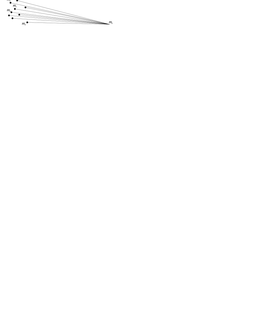
Figure 6.1: A system of $N$ massive bodies acting on particle $m_{0}$.

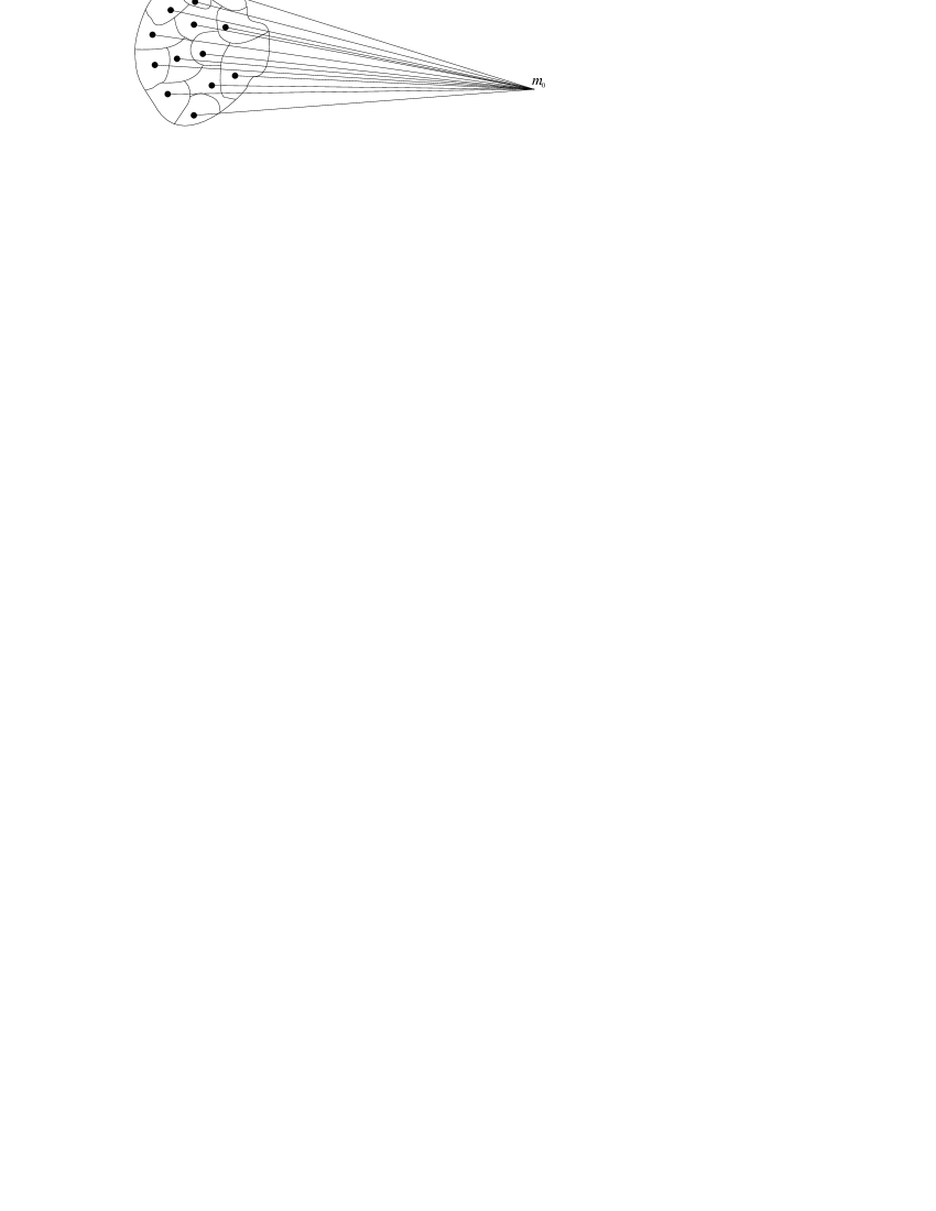
Figure 6.2: An extended body is split into a number of $N$ parts or cells. Each cell is then approximated by a point-like body situated at the center of mass of the cell and having mass $m_{i}$ equal to the mass of the cell. In this way the extended body is approximated by a system of $N$ point-like bodies.

Let us now consider an extended body with some continuous mass distribution. The task is to calculate its gravitational potential at a point lying outside of the body. We can split the whole body into $N$ parts or “cells” with some arbitrary $N\geq 1$ (see Fig. 6.2). Now, if as an approximation, we replace each cell by a point-like body situated at the center of mass of the cell and having mass $m_{i}$ equal to the mass of the cell, we get a system of $N$ point-like bodies instead of the extended body. The gravitational potential of such a system is again given by (6.2). Clearly, the larger is the number of cells $N$, the better is the approximation. In order to get the potential of an extended body we can simply consider the limit $N\to\infty$. It is clear that such a limit means mathematically that we proceed from a finite sum $\sum_{i=1}^{N}$ to an integral over the volume of the body $\int_{V}$. Masses $m_{i}$ of the cells should be replaced by mass elements $dm=\sigma d^{3}x$, where $\sigma$ is the mass density of the body (in general as function of time and position within the body) and $d^{3}x$ is the volume element. In this way one gets

$$U(t,{\mbox{\boldmath$x$}})=\int_{V}{G\,dm\over\rho}=\int_{V}{G\,\sigma(t,{\mbox{\boldmath$x$}}^{\prime})\,d^{3}x^{\prime}\over|{\mbox{\boldmath$x$}}-{\mbox{\boldmath$x$}}^{\prime}|},$$ (6.3)

where the integration goes over all points ${\mbox{\boldmath$x$}}^{\prime}$ inside the body (that is, where $\sigma>0$). This equation is valid for any point $x$ at which the potential is evaluated irrespective if $x$ is situated inside or outside the body. However, in the following we consider only points $x$ lying outside of the body. Mathematically this can be written as follows. For any body there exists such a radius $R$ so that for each points $x$ such that $|{\mbox{\boldmath$x$}}|>R$ the density $\sigma$ of the body vanishes:

$$\exists\,R:\,\forall\,{\mbox{\boldmath$x$}}:\,|{\mbox{\boldmath$x$}}|>R,\ \sigma(t,{\mbox{\boldmath$x$}})=0\,.$$ (6.4)

Radius $R$ can be called maximal radius of the body in the selected reference system. In the following we consider $U(t,{\mbox{\boldmath$x$}})$ only for such $x$ that $|{\mbox{\boldmath$x$}}|>R$. It is easy to see that in this case function $U(t,{\mbox{\boldmath$x$}})$ defined by (6.3) satisfies the Laplace equation

$$\Delta\,U(t,{\mbox{\boldmath$x$}})=0,$$ (6.5)

where $\Delta$ is the Laplace operator defined for any function $f$ as

$$\Delta\,f={\partial^{2}\over\partial x^{2}}\,f+{\partial^{2}\over\partial y^{2}}\,f+{\partial^{2}\over\partial z^{2}}\,f\,.$$ (6.6)

One can check directly that $U(t,{\mbox{\boldmath$x$}})$ defined by (6.3) satisfies (6.5). Indeed, considering that vectors $x$ and ${\mbox{\boldmath$x$}}^{\prime}$ have components $(x,y,z)$ and $(x^{\prime},y^{\prime},z^{\prime})$, respectively, one gets

$${\partial U\over\partial x}=-\int_{V}\,G\,\sigma(t,{\mbox{\boldmath$x$}}^{\prime})\,{x-x^{\prime}\over|{\mbox{\boldmath$x$}}-{\mbox{\boldmath$x$}}^{\prime}|}\,d^{2}x^{\prime}$$ (6.7)

and

$${\partial^{2}U\over\partial x^{2}}=\int_{V}\,G\,\sigma(t,{\mbox{\boldmath$x$}}^{\prime})\,{3\,(x-x^{\prime})^{2}-|{\mbox{\boldmath$x$}}-{\mbox{\boldmath$x$}}^{\prime}|^{2}\over|{\mbox{\boldmath$x$}}-{\mbox{\boldmath$x$}}^{\prime}|^{5}}\,d^{2}x^{\prime}\,,$$ (6.8)

and analogous for ${\partial^{2}U\over\partial y^{2}}$ and ${\partial^{2}U\over\partial z^{2}}$. Summing up ${\partial^{2}U\over\partial x^{2}}$, ${\partial^{2}U\over\partial y^{2}}$ and ${\partial^{2}U\over\partial z^{2}}$ one sees that (6.5) is satisfied. Functions satisfying Laplace equation are called harmonic functions. Therefore, one can say that the gravitational potential of an extended body is harmonic function outside of the body.

Now let us turn to the calculation of $U(t,{\mbox{\boldmath$x$}})$ for a given body. If density $\sigma$ is given, for any given $t$ and $x$ the potential $U$ can in principle be calculated by numerical integration of (6.3). The involved integral over the volume is a three-dimensional integral and its calculation is rather complicated. For each $x$ the integral should be computed anew and this is extremely inconvenient. It turns out, however, that this integral can be represented in such a way that the whole dependence on $x$ is explicit. Let us write

$${1\over|{\mbox{\boldmath$x$}}-{\mbox{\boldmath$x$}}^{\prime}|}={1\over\sqrt{r^{2}+r^{\prime 2}-2\,r\,r^{\prime}\,\cos H}},$$ (6.9)

where $r=|{\mbox{\boldmath$x$}}|$, $r^{\prime}=|{\mbox{\boldmath$x$}}^{\prime}|$ and $0\leq H\leq\pi$ is the angle between vectors $x$ and ${\mbox{\boldmath$x$}}^{\prime}$ (see Fig. 6.3). Denoting $\displaystyle{r^{\prime}\over r}=z$ and $\cos H=x$ ($-1\leq x\leq 1$) one can write

$${1\over|{\mbox{\boldmath$x$}}-{\mbox{\boldmath$x$}}^{\prime}|}={1\over\sqrt{r^{2}+r^{\prime 2}-2\,r\,r^{\prime}\,\cos H}}={1\over r}\,{1\over\sqrt{1+z^{2}-2\,x\,z}}.$$ (6.10)

Note that notations $x$ and $z$ have now nothing to do with the components of vector $x$. Since we only consider points with $r=|{\mbox{\boldmath$x$}}|>R$ and since for any point of the body $r^{\prime}=|{\mbox{\boldmath$x$}}^{\prime}|\leq R$, one has $z<1$.

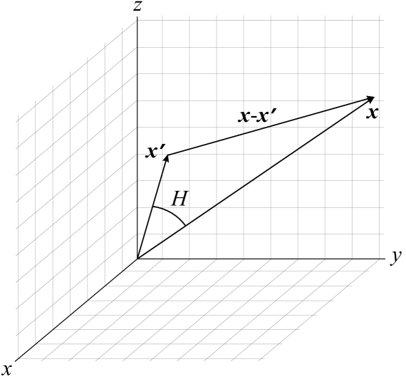
Figure 6.3: Point ${\mbox{\boldmath$x$}}^{\prime}$ is situated within the body, while point $x$ outside of it. The distance between two points is given by $|{\mbox{\boldmath$x$}}-{\mbox{\boldmath$x$}}^{\prime}|$ and the angles between vectors $x$ and ${\mbox{\boldmath$x$}}^{\prime}$ is denoted by $H$ ($0\leq H\leq\pi$).

6.1.2 Legendre polynomials

Mathematically, the second factor on the right-hand side of (6.10) can be expanded as

$${1\over\sqrt{1+z^{2}-2\,x\,z}}=\sum_{n=0}^{\infty}P_{n}(x)\,z^{n}\,,$$ (6.11)

where $P_{n}(x)$ are the so-called Legendre polynomials. The left-hand side of (6.11) is called generating function for the Legendre polynomials. Direct calculations show that

$${1\over\sqrt{1+z^{2}-2\,x\,z}}=1+x\,z+{3\,x^{2}-1\over 2}\,z^{2}+O(z^{3})\,.$$ (6.12)

This allows one derive explicitly lower-order polynomials $P_{n}$:

$$P_{0}(x) = 1\,,$$

$$P_{1}(x) = x\,,$$

$$P_{2}(x) = {3\over 2}\,x^{2}-{1\over 2}\,.$$ (6.13)

In principle, computing higher-order terms in (6.12) directly one can derive higher-order Legendre polynomials. However, the amount of computational work grows very quickly and it is much better to proceed differently. Let us derive recurrent relations for $P_{n}(x)$ starting from their definition (6.11). To this end let us compute the derivative of (6.11) with respect to $z$:

$${d\over dz}\,{1\over\sqrt{1+z^{2}-2\,x\,z}}={d\over dz}\,\sum_{n=0}^{\infty}P_{n}(x)\,z^{n}\,.$$ (6.14)

This gives

$${x-z\over\left(\sqrt{1+z^{2}-2\,x\,z}\right)^{3}}=\sum_{n=0}^{\infty}n\,P_{n}(x)\,z^{n-1}$$ (6.15)

or multiplying both sides by $1+z^{2}-2\,x\,z$

$${x-z\over\sqrt{1+z^{2}-2\,x\,z}}=(1+z^{2}-2\,x\,z)\,\sum_{n=0}^{\infty}n\,P_{n}(x)\,z^{n-1}\,.$$ (6.16)

Using again (6.11) in the left-hand side one finally gets

$$(x-z)\,\sum_{n=0}^{\infty}P_{n}(x)\,z^{n}=(1+z^{2}-2\,x\,z)\,\sum_{n=0}^{\infty}n\,P_{n}(x)\,z^{n-1}\,.$$ (6.17)

Now, since this equations must be satisfied identically (that is, for any $z$), the idea is to equate the coefficients at equal powers of $z$ on the left-hand and right-hand sides of (6.17). Expanding (6.17) one gets

$$\phantom{=}\sum_{n=0}^{\infty}x\,P_{n}(x)\,z^{n}-\sum_{n=0}^{\infty}P_{n}(x)\,z^{n+1}$$

$$=\sum_{n=0}^{\infty}n\,P_{n}(x)\,z^{n-1}+\sum_{n=0}^{\infty}n\,P_{n}(x)\,z^{n+1}-\sum_{n=0}^{\infty}2\,n\,x\,P_{n}(x)\,z^{n}\,.$$ (6.18)

Using that

$$\sum_{n=0}^{\infty}P_{n}(x)\,z^{n+1} = \sum_{n=1}^{\infty}P_{n-1}(x)\,z^{n}\,,$$ (6.19)

$$\sum_{n=0}^{\infty}n\,P_{n}(x)\,z^{n-1} = \sum_{n=0}^{\infty}(n+1)\,P_{n+1}(x)\,z^{n}\,,$$ (6.20)

$$\sum_{n=0}^{\infty}n\,P_{n}(x)\,z^{n+1} = \sum_{n=1}^{\infty}(n-1)\,P_{n-1}(x)\,z^{n}$$ (6.21)

one gets

$$\phantom{=}\sum_{n=0}^{\infty}x\,P_{n}(x)\,z^{n}-\sum_{n=1}^{\infty}P_{n-1}(x)\,z^{n}$$

$$=\sum_{n=0}^{\infty}(n+1)\,P_{n+1}(x)\,z^{n}+\sum_{n=1}^{\infty}(n-1)\,P_{n-1}(x)\,z^{n}-\sum_{n=0}^{\infty}2\,n\,x\,P_{n}(x)\,z^{n}\,.$$ (6.22)

Now, equating the coefficients at equal powers of $z$ one gets

$$x\,P_{0}(x)=P_{1}(x),\ {\rm for}\ n=0\,,$$ (6.23)

$$x\,P_{n}(x)-P_{n-1}(x)=(n+1)P_{n+1}(x)+(n-1)P_{n-1}(x)-2nxP_{n}(x),\ {\rm for}\ n>0\,.$$ (6.24)

From (6.1.2) one can see that the first equation is satisfied by $P_{0}(x)$ and $P_{1}(x)$ and, therefore, gives no additional information. The second equation can be written as

$$(n+1)\,P_{n+1}(x)=(2\,n+1)\,x\,P_{n}(x)-n\,P_{n-1}(x),\quad n\geq 1\,.$$ (6.25)

This equation allows one to compute $P_{n}(x)$ for a given $x$ if $P_{n-1}(x)$ and $P_{n-2}(x)$ are given. This means that, starting from $P_{0}(x)=1$ and $P_{1}(x)=x$ as given by (6.1.2), $P_{n}(x)$ can be computed for any $x$ and $n\geq 2$. Below we will need also the following properties of Legendre polynomials:

$$P_{n}(-x)=(-1)^{n}\,P_{n}(x)\,,$$ (6.26)

$$\int_{-1}^{1}P_{n}(x)P_{m}(x)dx=\biggl{[}\matrix{0,\quad n\neq m\cr{2\over 2n+1},\quad n=m}\,.$$ (6.27)

Eq. (6.26) means that the Legendre polynomials $P_{n}$ are even functions of $x$ for even $n$ and odd functions for odd $n$. For $n=0$ and $n=1$ this relation can be seen directly. For $n>1$ it is easy to prove (6.26) from the recurrent formula (6.25).

Exercise. Prove (6.26) from (6.25) for $n>1$ using that (6.26) is correct for $n=0$ and $n=1$.

The proof of (6.27) and further properties of Legendre polynomials can be found, e.g., in Chapter 8 of Abramowitz & Stegun (1965). Fig. 6.4 shows several first Legendre polynomials. One can prove that $-1\leq P_{n}(x)\leq 1$ for any $n$.

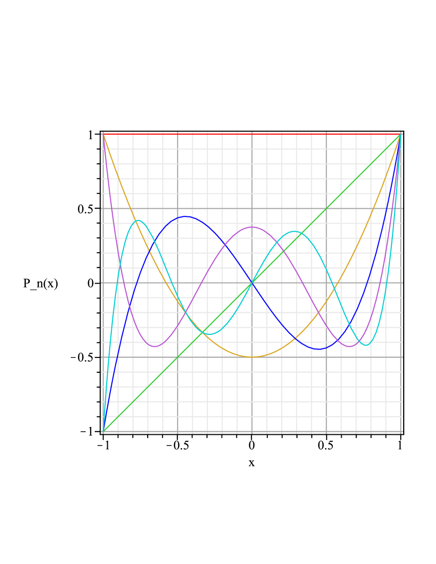
Figure 6.4: Legendre polynomials $P_{n}(x)$ are shown here for $-1\leq x\leq 1$ and for $n=0,1,\dots,5$ (red, green, brown, dark blue, magenta and light blue, respectively).

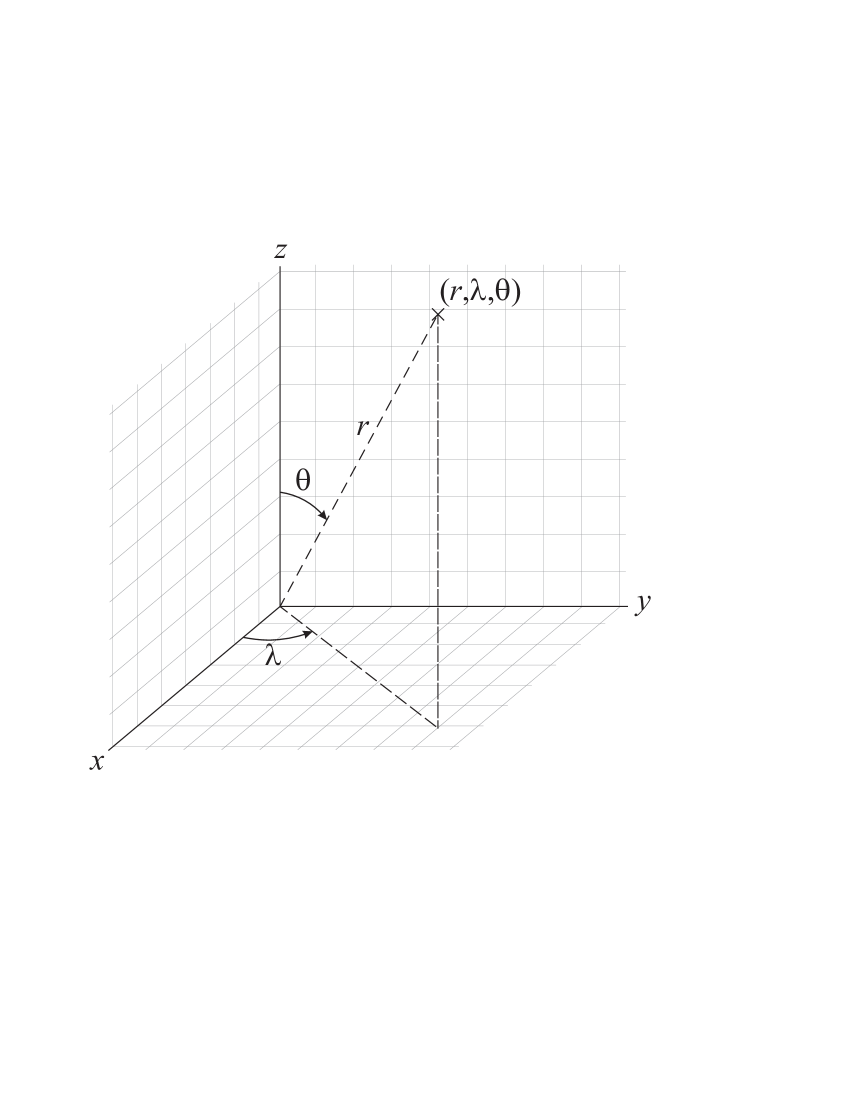
Figure 6.5: Definition of the spherical coordinates: longitude $\lambda$ ($0\leq\lambda\leq 2\pi$) and co-latitude $\theta$ ($0\leq\theta\leq\pi$).

6.1.3 Expansion of the potential

Using the expansion (6.11) in (6.10) the potential (6.3) can be written as

$$U=\sum_{n=0}^{\infty}{1\over r^{n+1}}\,\int_{V}{r^{\prime}}^{n}\,P_{n}(\cos H)\,G\,\sigma(t,{\mbox{\boldmath$x$}}^{\prime})\,d^{3}x^{\prime}\,.$$ (6.28)

Here we have reached our goal – to get an expression for $U(t,{\mbox{\boldmath$x$}})$ in which the dependence on $x$ is explicit – only partially. Indeed, the dependence on $r=|{\mbox{\boldmath$x$}}|$ is explicitly written since all quantities under the integral are independent of $r$. On the other hand $\cos H$ under the integral does depend on the orientation of $x$, that is, on the unit vector ${\mbox{\boldmath$x$}}/r$. Such unit vector can be characterized for example by the corresponding spherical coordinates. Introducing longitude $\lambda$ ($0\leq\lambda\leq 2\pi$) and co-latitude $\theta$ ($0\leq\theta\leq\pi$) (see Fig. 6.5) – one has

$$\cos H=\cos\theta\,\cos\theta^{\prime}+\sin\theta\,\sin\theta^{\prime}\,\cos(\lambda-\lambda^{\prime}),$$ (6.29)

where $\lambda$ and $\theta$ correspond to $x$ while $\lambda^{\prime}$ and $\theta^{\prime}$ correspond to ${\mbox{\boldmath$x$}}^{\prime}$. This formula can be easily derived using

$${\mbox{\boldmath$x$}}=\pmatrix{r\,\cos\lambda\,\sin\theta\cr r\,\sin\lambda\,\sin\theta\cr r\,\cos\theta}\,,$$ (6.30)

similar formula for ${\mbox{\boldmath$x$}}^{\prime}$, and noting that $\cos H=\displaystyle{{\mbox{\boldmath$x$}}\cdot{\mbox{\boldmath$x$}}^{\prime}\over r\,r^{\prime}}$, where ’$\cdot$’ denotes scalar product of two vectors. Furthermore, one has

$$P_{n}(\cos H)=\sum_{k=0}^{n}(2-\delta_{k0})\,{(n-k)!\over(n+k)!}\,P_{nk}(\cos\theta)\,P_{nk}(\cos\theta^{\prime})\,\cos k(\lambda-\lambda^{\prime}),$$ (6.31)

where

$$\delta_{k0}=\biggl{[}\matrix{1,\quad k=0\cr 0,\quad k>0}$$ (6.32)

and $P_{nk}(x)$ are the associated Legendre polynomials defined as

$$P_{nk}(x)={\left(1-x^{2}\right)}^{k/2}\,{d^{k}\over dx^{k}}\,P_{n}(x),\quad 0\leq k\leq n.$$ (6.33)

Clearly, $P_{n0}(x)=P_{n}(x)$. Mathematical proof of (6.31) and further properties of the associated Legendre polynomials can be found, e.g., in Chapter 8 of Abramowitz & Stegun (1965). Note that in the literature one can find different sign conventions related to the associated Legendre polynomials, in particular regarding an additional factor $(-1)^{k}$.

Substituting (6.31) into (6.28) one finally gets the expansion of the gravitational potential of an extended body in the form

$$U=\sum_{n=0}^{\infty}\sum_{k=0}^{n}\,G\,{P_{nk}(\cos\theta)\over r^{n+1}}\,\left(C_{nk}\cos k\lambda+S_{nk}\sin k\lambda\right).$$ (6.34)

Coefficients $C_{nk}$ and $S_{nk}$ are real numbers that fully characterize the gravitational potential of the body and defined as

$$C_{nk}=(2-\delta_{k0})\,{(n-k)!\over(n+k)!}\,\int_{V}{r^{\prime}}^{n}\,P_{nk}(\cos\theta^{\prime})\,\cos k\lambda^{\prime}\,\sigma(t,{\mbox{\boldmath$x$}}^{\prime})\,d^{3}x^{\prime}\,,$$ (6.35)

$$S_{nk}=(2-\delta_{k0})\,{(n-k)!\over(n+k)!}\,\int_{V}{r^{\prime}}^{n}\,P_{nk}(\cos\theta^{\prime})\,\sin k\lambda^{\prime}\,\sigma(t,{\mbox{\boldmath$x$}}^{\prime})\,d^{3}x^{\prime}\,.$$ (6.36)

It is clear that $C_{nk}$ and $S_{nk}$ do not depend on $x$, but only on the mass distribution inside the body. Coefficient $S_{n0}=0$ for any $n$ because of the factor $\sin k\lambda^{\prime}$ under the integral in its definition (the latter factor vanishes for $k=0$). One has, therefore, $2n+1$ coefficients $C_{nk}$ and $S_{nk}$ characterizing the gravitational field of an extended body for each $n$. Note that $C_{nk}$ and $S_{nk}$ are not dimensionless. Their dimensionality is ${\rm kg}\cdot{\rm m}^{n}$.

The expansion (6.34) for $U(t,{\mbox{\boldmath$x$}})$ gives explicitly the dependence of $U$ on the point $x$ at which $U$ should be evaluated. This is done using spherical coordinates $(r,\lambda,\theta)$ of $x$. We have thus achieved our goal.

6.2 First terms of the expansion

Summary: The mass of the body. The relations between the potential and the choice of the origin and the orientation of the coordinate system.

Up to now the reference system where we described the body and its gravitational potential $U$ was arbitrary. Here we show that the lower-order terms in (6.34) are closely related to the choice of the origin and the orientation of the reference system. In the following we consider that $\displaystyle{U=\sum_{n=0}^{\infty}U_{n}}$, where $U_{n}$ are all terms in (6.34) or (6.28) corresponding to a given $n$, that is

$$U_{n} = {1\over r^{n+1}}\,G\,\int_{V}{r^{\prime}}^{n}\,P_{n}(\cos H)\,\sigma(t,{\mbox{\boldmath$x$}}^{\prime})\,d^{3}x^{\prime}$$ (6.37)

$$= \sum_{k=0}^{n}\,G\,{P_{nk}(\cos\theta)\over r^{n+1}}\,\left(C_{nk}\cos k\lambda+S_{nk}\sin k\lambda\right)\,.$$

Note that $U_{n}$ is the part of potential $U$ falling off as $\displaystyle{1\over r^{n+1}}$ for $r$ going to infinity.

6.2.1 The term for $n=0$

For $n=0$ the first line of (6.37) gives (note that $P_{0}(\cos H)=1$)

$$U_{0}={1\over r}\,\int_{V}G\,\sigma(t,{\mbox{\boldmath$x$}}^{\prime})\,d^{3}x^{\prime}={G\,M\over r}\,,$$ (6.38)

where $M=\int_{V}\sigma(t,{\mbox{\boldmath$x$}}^{\prime})\,d^{3}x^{\prime}$ is the total mass of the body. From the second line of (6.37) we see that for $n=0$ there is only one coefficient $C_{00}$. Definition (6.35) again shows that

$$C_{00}=M\,.$$ (6.39)

Thus, we get an important result: the main $r^{-1}$ term of the gravitational potential of an arbitrary extended body is the same as if the body would be a mass point with mass $M$ equal to the total mass of the extended body. This term cannot be affected by any change of the reference system.

6.2.2 The terms for $n=1$

For $n=1$ the first line of (6.37) gives (note that $P_{1}(\cos H)=\cos H$ and $r^{\prime}\,\cos H=\displaystyle{{\mbox{\boldmath$x$}}\cdot{\mbox{\boldmath$x$}}^{\prime}\over r}$)

$$U_{1}={1\over r^{2}}\,G\,\int_{V}{{\mbox{\boldmath$x$}}\cdot{\mbox{\boldmath$x$}}^{\prime}\over r}\,\sigma(t,{\mbox{\boldmath$x$}}^{\prime})\,d^{3}x^{\prime}={G\,M\over r^{3}}\,{\mbox{\boldmath$x$}}\cdot{\mbox{\boldmath$x$}}_{c},$$ (6.40)

where ${\mbox{\boldmath$x$}}_{c}=\displaystyle{{1\over M}\,\int_{V}\sigma(t,{\mbox{\boldmath$x$}}^{\prime})\,{\mbox{\boldmath$x$}}^{\prime}\,d^{3}x^{\prime}}$ are the coordinates of the center of mass of the body in the chosen reference system. On the other hand, considering the second line of (6.37) one sees that $U_{1}$ is characterized by $C_{10}$, $C_{11}$, and $S_{11}$ (recall that $S_{n0}=0$ for any $n$). These three coefficients are equivalent to the three components of ${\mbox{\boldmath$x$}}_{c}$. Indeed, it is easy to see that

$$C_{10} = M\,z_{c}\,,$$

$$C_{11} = M\,x_{c}\,,$$

$$S_{11} = M\,y_{c}\,,$$ (6.41)

where $(x_{c},y_{c},z_{c})$ are the components of vector ${\mbox{\boldmath$x$}}_{c}$. It is clear that choosing the reference system in such a way that its origin coincides with the center of mass of the body under study, one gets ${\mbox{\boldmath$x$}}_{c}=0$. In this case, we have $U_{1}=0$ and, therefore, $C_{10}=C_{11}=S_{11}=0$. Usually, this possibility is indeed used and one puts $C_{10}$, $C_{11}$, $S_{11}$ to zero.

6.2.3 The terms for $n=2$

For $n=2$ the first line of (6.37) gives (note that $P_{2}(\cos H)={3\over 2}\cos^{2}H-{1\over 2}$)

$$U_{2} = {1\over r^{3}}\,G\,\int_{V}{r^{\prime}}^{2}\left({3\over 2}\cos^{2}H-{1\over 2}\right)\,\sigma(t,{\mbox{\boldmath$x$}}^{\prime})\,d^{3}x^{\prime}$$ (6.42)

$$= {1\over r^{3}}\,G\,\int_{V}{3\,{\left({\mbox{\boldmath$x$}}\cdot{\mbox{\boldmath$x$}}^{\prime}\right)}^{2}-r^{2}\,{r^{\prime}}^{2}\over 2\,r^{2}}\,\sigma(t,{\mbox{\boldmath$x$}}^{\prime})\,d^{3}x^{\prime}$$

$$= -{3\over 2}\,G\,\sum_{i=1}^{3}\sum_{j=1}^{3}\hat{I}^{ij}\,{x^{i}\,x^{j}\over r^{5}}\,,$$

where $\hat{I}^{ij}$ is the trace-free part of the tensor of inertia $I^{ij}$ of the body. Namely, $\hat{I}^{ij}=I^{ij}-{1\over 3}\,\delta^{ij}\,I^{kk}$, where $I^{kk}=I^{11}+I^{22}+I^{33}$ is the trace of $I^{ij}$ and $\delta^{ij}$ are the components of identity matrix ($\delta^{ij}=1$ for $i=j$ and $\delta^{ij}=0$ for $i\neq j$). The tensor of inertia $I^{ij}$ has its usual definition

$$I^{ij}=\int_{V}\left(\delta^{ij}\,|{\mbox{\boldmath$x$}}|^{2}-x^{i}\,x^{j}\right)\,\sigma(t,{\mbox{\boldmath$x$}})\,d^{3}x\,.$$ (6.43)

For $n=2$ there are five coefficients $C_{nk}$ and $S_{nk}$: $C_{20}$, $C_{21}$, $C_{22}$, $S_{21}$, and $S_{22}$. On the other hand the symmetric trace-free matrix $\hat{I}^{ij}$ can be written as

$$\hat{I}^{ij}=-M\,R^{2}\,\pmatrix{a&b&c\cr b&d&e\cr c&e&-a-d}$$ (6.44)

and also has five independent components. Dimensionless numbers $a$, $b$, $c$, $d$ and $e$ fully characterize the gravitational potential $U_{2}$ and are directly related to the five coefficients $C_{20}$, $C_{21}$, $C_{22}$, $S_{21}$, and $S_{22}$. One can demonstrate that

$$C_{20} = -{3\over 2}\,(a+d)\,M\,R^{2}\,,$$

$$C_{21} = c\,M\,R^{2}\,,$$

$$C_{22} = {1\over 4}\,(a-d)\,M\,R^{2}\,,$$

$$S_{21} = e\,M\,R^{2}\,,$$

$$S_{22} = {1\over 2}\,b\,M\,R^{2}$$ (6.45)

or inverting

$$M\,R^{2}\,a = -{1\over 3}\,C_{20}+2\,C_{22}\,,$$

$$M\,R^{2}\,b = 2\,S_{22}\,,$$

$$M\,R^{2}\,c = C_{21}\,,$$

$$M\,R^{2}\,d = -{1\over 3}\,C_{20}-2\,C_{22}\,,$$

$$M\,R^{2}\,e = S_{21}\,.$$ (6.46)

Since we consider rectangular Cartesian right-handed system there are only two sorts of freedom to define it. First, the choice of the origin used for $n=1$ above. Second, the choice of spatial orientation of the axes. Clearly, the components of $\hat{I}^{ij}$ depend on the orientation of the coordinate system. Generally, a rotation in three-dimensional space is defined by three parameters. Therefore, three coefficients among $C_{20}$, $C_{21}$, $C_{22}$, $S_{21}$, and $S_{22}$ can be made zero by choosing some special orientation of the coordinate system. For example, the matrix $\hat{I}^{ij}$ can be diagonalized by a suitable rotation to get $C_{21}$, $S_{21}$ and $S_{22}$ to zero (see (6.2.3) and consider that for a diagonal matrix $b=c=e=0$ in (6.44)). More detailed analysis shows that the orientation can be chosen in such a way that $C_{21}$, $S_{21}$ and either $C_{22}$ or $S_{22}$ vanish. This possibility is usually not used since the orientation of the reference system is fixed from the consideration of continuity and convenience.

Let us note that it makes no sense to consider separately terms $U_{n}$ for $n>2$ since the freedom in the definition of the coordinate system is already exhausted.

6.3 Symmetric bodies

Summary: Axial symmetry. Axial symmetry and the symmetry between the north and the south. Spherical symmetry. Symmetry with respect to three coordinate planes.

In this Section we will simplify the general expansion (6.34) for the gravitational potential $U$ for the case of extended bodies having several sorts of symmetries. This consideration allows one to understand which coefficients $C_{nk}$ and $S_{nk}$ describe which properties of the mass distribution within the body.

6.3.1 Axial symmetry

Let us first consider a body that is symmetric with respect to some axis and let us choose that symmetry axis as z-axis of our coordinate system. Then the symmetry means that the density $\sigma$ does not depend on the spherical coordinate $\lambda$ (see Fig. 6.5): $\sigma\neq\sigma(\lambda)$. Therefore, $\sigma=\sigma(t,r,\theta)$ and the integrals (6.35)–(6.36) can be written as

$$C_{nk} = (2-\delta_{k0})\,{(n-k)!\over(n+k)!}\,$$ (6.47)

$$\times\left(\int_{0}^{R}dr^{\prime}{r^{\prime}}^{n+2}\int_{0}^{\pi}d\theta^{\prime}\sin\theta^{\prime}\,P_{nk}(\cos\theta^{\prime})\,\sigma(t,r^{\prime},\theta^{\prime})\right)\times\left(\int_{0}^{2\pi}d\lambda^{\prime}\,\cos k\lambda^{\prime}\right)\,,$$

$$S_{nk} = (2-\delta_{k0})\,{(n-k)!\over(n+k)!}\,$$ (6.48)

$$\times\left(\int_{0}^{R}dr^{\prime}{r^{\prime}}^{n+2}\int_{0}^{\pi}d\theta^{\prime}\sin\theta^{\prime}\,P_{nk}(\cos\theta^{\prime})\,\sigma(t,r^{\prime},\theta^{\prime})\right)\times\left(\int_{0}^{2\pi}d\lambda^{\prime}\,\sin k\lambda^{\prime}\right)\,.$$

Here we used the expression for the volume element in spherical coordinates: $d^{3}x^{\prime}={r^{\prime}}^{2}\,\sin\theta^{\prime}\,dr^{\prime}\,d\theta^{\prime}\,d\lambda^{\prime}$. The last integral in (6.47)–(6.48) over $d\lambda^{\prime}$ is zero for any $k$ in $S_{nk}$ and for $k>0$ in $C_{nk}$. Therefore, for an axially symmetric body $C_{nk}=0$ for $k>0$ and $S_{nk}=0$ for any $k$. This holds for any $n$. It means that only coefficients $C_{n0}$ are not zero and fully characterize the gravitational field of the body. The expansion of $U$ in this case takes the form

$$U=\sum_{n=0}^{\infty}\,G\,C_{n0}\,{P_{n}(\cos\theta)\over r^{n+1}}\,.$$ (6.49)

Therefore, we conclude that $C_{nk}$ for any $n$ and $k>0$ and $S_{nk}$ for any $n$ and $k$ characterize the deviation of the body from axial symmetry.

6.3.2 Axial symmetry and the symmetry about $xy$-plane

Let us now consider the case when, in addition to the axial symmetry (about $z$-axis), the body is symmetric about the $xy$-plane (one can speak also of “symmetry between the north and the south”). In this case density has the property that $\sigma(t,r,\theta)=\sigma(t,r,\pi-\theta)$. Using (6.47) for $k=0$ one gets

$$C_{n0} = 2\pi\,\int_{0}^{R}dr^{\prime}{r^{\prime}}^{n+2}\int_{0}^{\pi}d\theta^{\prime}\sin\theta^{\prime}\,P_{n}(\cos\theta^{\prime})\,\sigma(t,r^{\prime},\theta^{\prime})\,,$$ (6.50)

The integral over $d\theta^{\prime}$ can be split into two parts:

$$\int_{0}^{\pi/2}d\theta^{\prime}\sin\theta^{\prime}\,P_{n}(\cos\theta^{\prime})\,\sigma(t,r^{\prime},\theta^{\prime})+\int_{\pi/2}^{\pi}d\theta^{\prime}\sin\theta^{\prime}\,P_{n}(\cos\theta^{\prime})\,\sigma(t,r^{\prime},\theta^{\prime})\,.$$ (6.51)

Now, using the symmetry of the body one can show that these two integrals are related to each other. Indeed, let us introduce $\widetilde{\theta}^{\prime}=\pi-\theta^{\prime}$ and replace $\theta^{\prime}$ through $\widetilde{\theta}^{\prime}$ in the integral from $\pi/2$ to $\pi$:

$$\int_{\pi/2}^{\pi}d\theta^{\prime}\sin\theta^{\prime}\,P_{n}(\cos\theta^{\prime})\,\sigma(t,r^{\prime},\theta^{\prime})$$

$$\qquad=-\int_{\pi/2}^{0}d\widetilde{\theta}^{\prime}\sin\widetilde{\theta}^{\prime}\,(-1)^{n}\,P_{n}(\cos\widetilde{\theta}^{\prime})\,\sigma(t,r^{\prime},\widetilde{\theta}^{\prime})$$

$$\qquad=(-1)^{n}\,\int_{0}^{\pi/2}d\widetilde{\theta}^{\prime}\sin\widetilde{\theta}^{\prime}\,P_{n}(\cos\widetilde{\theta}^{\prime})\,\sigma(t,r^{\prime},\widetilde{\theta}^{\prime})$$

$$\qquad=(-1)^{n}\,\int_{0}^{\pi/2}d\theta^{\prime}\sin\theta^{\prime}\,P_{n}(\cos\theta^{\prime})\,\sigma(t,r^{\prime},\theta^{\prime}).$$

Here we used that $d\theta^{\prime}=-d\widetilde{\theta}^{\prime}$, $\sigma(t,r^{\prime},\theta^{\prime})=\sigma(t,r^{\prime},\pi-\widetilde{\theta}^{\prime})=\sigma(t,r^{\prime},\widetilde{\theta}^{\prime})$, $\sin\theta^{\prime}=\sin(\pi-\widetilde{\theta}^{\prime})=\sin\widetilde{\theta}^{\prime}$, $\cos\theta^{\prime}=\cos(\pi-\widetilde{\theta}^{\prime})=-\cos\widetilde{\theta}^{\prime}$, and that, according to (6.26), $P_{n}(-\cos\widetilde{\theta}^{\prime})=(-1)^{n}\,P_{n}(\cos\widetilde{\theta}^{\prime})$. Finally, for the boundaries of integration we get that $\theta^{\prime}=\pi/2$ and $\theta^{\prime}=\pi$ correspond to $\widetilde{\theta}^{\prime}=\pi/2$ and $\widetilde{\theta}^{\prime}=0$, respectively. In the last equality we simply replaced $\widetilde{\theta}^{\prime}$ by $\theta^{\prime}$ as a change of notation.

It is, therefore, clear that with this symmetry $C_{n0}=0$ for odd $n$. The expansion of $U$ thus reads

$$U=\sum_{n=0}^{\infty}\,G\,C_{2n,0}\,{P_{2n}(\cos\theta)\over r^{2n+1}}\,.$$ (6.52)

We conclude that $C_{2n+1,0}$ characterize the deviation of the (axially symmetric) body from the symmetry about the $xy$-plane.

6.3.3 Spherical symmetry

We assume now an even stronger symmetry. Namely the spherical one. In this case the density only depends on the radial coordinate and dies not depend on $\lambda$ and $\theta$: $\sigma=\sigma(t,r)$. In this case from (6.50) one has

$$C_{n0} = 2\pi\,\left(\int_{0}^{R}dr^{\prime}{r^{\prime}}^{n+2}\sigma(t,r^{\prime})\right)\times\left(\int_{0}^{\pi}d\theta^{\prime}\sin\theta^{\prime}\,P_{n}(\cos\theta^{\prime})\right)\,,$$ (6.53)

The integral over $d\theta^{\prime}$ can be written as

$$\int_{0}^{\pi}d\theta^{\prime}\sin\theta^{\prime}\,P_{n}(\cos\theta^{\prime})=-\int_{0}^{\pi}P_{n}(\cos\theta^{\prime})\,d\cos\theta^{\prime}=-\int_{-1}^{1}P_{n}(s)\,ds,$$ (6.54)

where $s=\cos\theta^{\prime}$. According to (6.27) where we can put $m=0$ and $P_{m}(x)=1$ one gets

$$\int_{-1}^{1}P_{n}(s)\,ds=\left[\matrix{2,\quad n=0\cr 0,\quad n\geq 1}\right.\,.$$ (6.55)

Therefore, only $C_{00}=M$ (see Section 6.2.1) does not vanish for a spherical symmetric body and the gravitational field of a spherically symmetric body reads

$$U={G\,C_{00}\over r}={G\,M\over r}\,.$$ (6.56)

Note that we have now proved this formula for any spherically symmetric distribution of the density $\sigma=\sigma(t,r)$. This is a substantial generalization with respect to the case of point-like bodies. We conclude that $C_{nk}$ for $n>0$ and $S_{nk}$ for any $n$ and $k$ characterize the deviation of the body from the spherical symmetry.

6.3.4 Symmetry with respect to three coordinate planes

One more interesting case is a body symmetric with respect to all three coordinate planes: $xy$-plane, $xz$-plane and $yz$-plane. For example, a triaxial ellipsoid possesses such a symmetry. One can demonstrate that in this case the expansion of $U$ reads

$$U=G\,\sum_{n=0}^{\infty}\,{1\over r^{2n+1}}\sum_{k=0}^{n}\,C_{2n,2k}\,P_{2n,2k}(\cos\theta)\cos 2k\lambda\,.$$ (6.57)

We conclude that $C_{nk}$ with odd $n$ and/or $k$ and all $S_{nk}$ characterize the deviation of the body from the symmetry about all three coordinate planes. The proof of (6.57) can be found, e.g., in Chandrasekhar (1987).

6.4 Spherical functions and the classification of the coefficients

Summary: Definition of spherical functions. The expansion of the gravitational potential in terms of spherical functions. The principal part of the potential: spherically-symmetric gravitational field. Zonal coefficients. Sectorial and tesseral coefficients.

Expansion (6.34) is a special case of general expansion of an arbitrary complex function of spherical coordinates in terms of spherical functions. Namely, the factors $P_{nk}(\cos\theta)$, $\cos k\lambda$ and $\sin k\lambda$ can be combined into a single complex function:

$$Y_{nk}(\lambda,\theta)=(-1)^{k}\,\sqrt{{2n+1\over 4\pi}\,{(n-k)!\over(n+k)!}}\,P_{nk}(\cos\theta)\,e^{\buildrel\circ\over{\hbox{\rm\char 16\relax}}k\lambda}\,.$$ (6.58)

Note that $e^{\buildrel\circ\over{\hbox{\rm\char 16\relax}}k\lambda}=\cos k\lambda+\buildrel\circ\over{\hbox{\rm\char 16\relax}}\,\sin k\lambda$, $\buildrel\circ\over{\hbox{\rm\char 16\relax}}$ being the imaginary unit $\buildrel\circ\over{\hbox{\rm\char 16\relax}}=\sqrt{-1}$. Functions $Y_{nk}$ depend only on $\lambda$ and $\theta$ and are, therefore, defined on a sphere (the radius of which plays no role). The numerical factor under the square root in (6.58) is only for a specific normalization that the integral $\displaystyle{\int_{0}^{\pi}d\theta\,\sin\theta\,\int_{0}^{2\pi}d\lambda\,Y_{nk}(\lambda,\theta)\,Y^{*}_{n^{\prime}k^{\prime}}(\lambda,\theta)}$ is equal to 1 if $n=n^{\prime}$ and $k=k^{\prime}$ and vanishes otherwise (“$*$” meaning complex conjugate). This factor does not play any role in the following and will not be further discussed. Functions $Y_{nk}$ constitute full functional basis on a sphere. It means that any complex function $g(\lambda,\theta)$ defined on a sphere can be represented as

$$g(\lambda,\theta)=\sum_{l=0}^{\infty}\sum_{m=-l}^{l}\,A_{lm}\,Y_{lm}(\lambda,\theta),$$ (6.59)

where $A_{lm}$ are some complex numbers. If function $g(\lambda,\theta)$ is real, coefficients $A_{lm}$ have some symmetry properties so that the whole sum on the right-hand side of (6.59) remains real. Let us also note that since $\cos k\left(\lambda-{\pi\over 2k}\right)=\sin k\lambda$ the real and imaginary parts of $Y_{nk}$ are related to each other in a simple way: ${\mathfrak{Im}}\,Y_{nk}(\lambda,\theta)={\mathfrak{Re}}\,Y_{nk}\left(\lambda-{\pi\over 2k},\theta\right)$.

Spherical functions are convenient to discuss the character of the coefficients $C_{nk}$ and $S_{nk}$. The expansion (6.34) is often written in the form

$$U = {G\,M\over r}\,\left\{\,\left(1-\sum_{n=2}^{\infty}J_{n}\,{\left(R\over r\right)}^{n}\,P_{n}(\cos\theta)\right)\right.$$ (6.60)

$$\qquad\qquad\left.+\sum_{n=2}^{\infty}\sum_{k=1}^{n}\,{\left(R\over r\right)}^{n}\,P_{nk}(\cos\theta)\,\left(\overline{C}_{nk}\cos k\lambda+\overline{S}_{nk}\sin k\lambda\right)\right\},$$

where $R$, as before, is the radius of a sphere encompassing the body and $M=C_{00}$ is the total mass of the body. Here one uses the coordinate system the origin of which coincides with the center of mass of the body, so that all terms in (6.34) with $n=1$ vanish and do not appear in (6.60). Coefficients $J_{n}$, $\overline{C}_{nk}$ and $\overline{S}_{nk}$ are dimensionless real numbers that are trivially related to $C_{nk}$ and $S_{nk}$:

$$J_{n} = -{1\over M\,R^{n}}\,C_{n0}\,,$$ (6.61)

$$\overline{C}_{nk} = {1\over M\,R^{n}}\,C_{nk}\,,$$ (6.62)

$$\overline{S}_{nk} = {1\over M\,R^{n}}\,S_{nk}\,.$$ (6.63)

Coefficients $C_{nk}$ and $S_{nk}$ (or $J_{n}$, $\overline{C}_{nk}$ and $\overline{S}_{nk}$) can be divided into four parts:

• The main part of the potential $\displaystyle{GM\over r}$ corresponds to $C_{00}=M$ and to $Y_{00}={1\over\sqrt{4\pi}}={\rm const}$.

• The zonal harmonics $J_{n}$ or $C_{n0}$ correspond to $Y_{n0}=\sqrt{2n+1\over 4\pi}\,P_{n}(\cos\theta)$ that do not depend on $\lambda$ (see Fig. 6.6). For odd $n$ the coefficients $J_{n}$ characterize the oblateness of the body. For even $n$ they characterize the asymmetry of the body with respect to the $xy$-plane (that is, asymmetry between the north and the south). This has been discussed in Section 6.3.

• The sectorial harmonics $\overline{C}_{nn}$ and $\overline{S}_{nn}$ correspond to $Y_{nn}$ and describe the effects that depend only on longitude $\lambda$ (see Fig. 6.6).

• The tesseral harmonics $\overline{C}_{nk}$ and $\overline{S}_{nk}$ for $n\geq 2$ and $1\leq k<n$ correspond to $Y_{nk}$ with the same indices and describe the effects that depend both on longitude $\lambda$ and co-latitude $\theta$. The word ’tessera’ means ’four’ or ’rectangle’. The surface of a sphere with $Y_{nk}$ plotted on it appears to be divided into various “rectangles” (see Fig. 6.6).

In general, the coefficients with larger $n$ and $k$ describes finer details of the potential $U$.

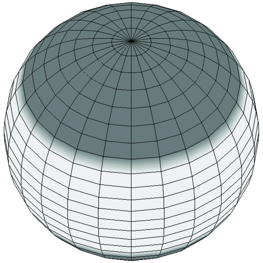
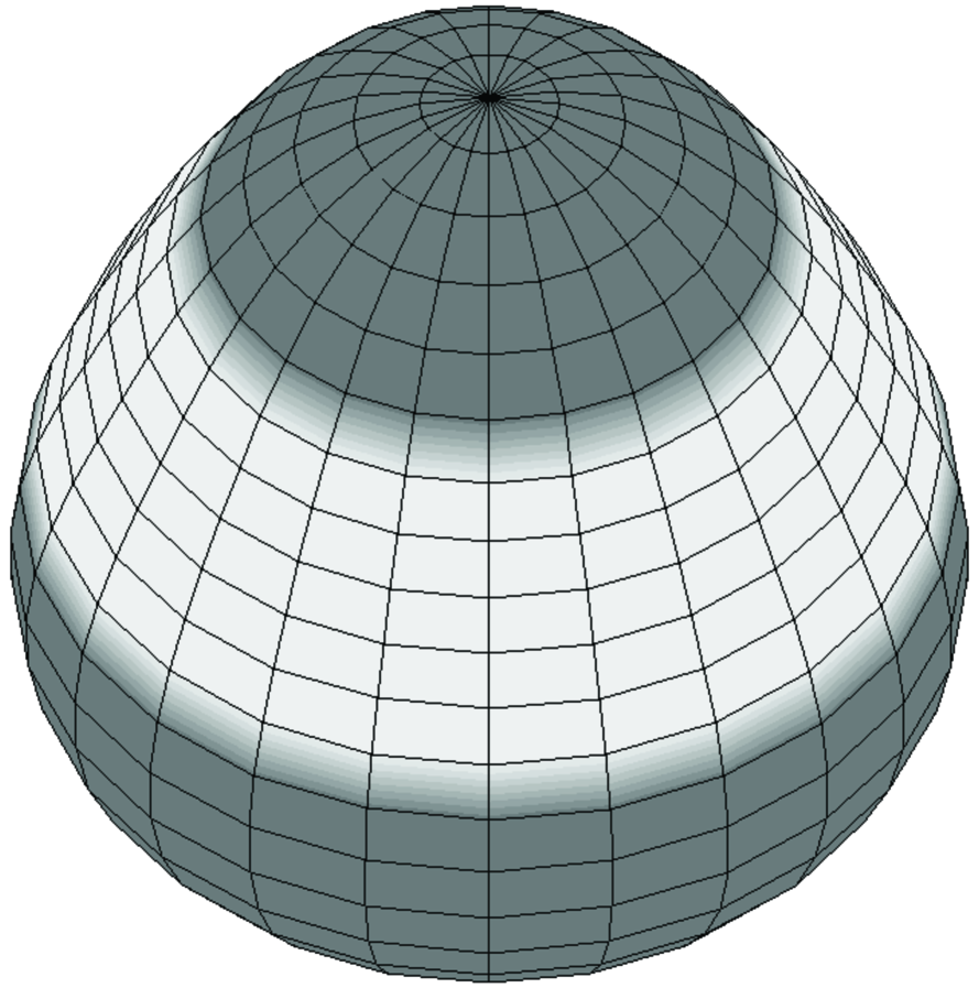
$n=2$ $k=0$	$n=3$ $k=0$
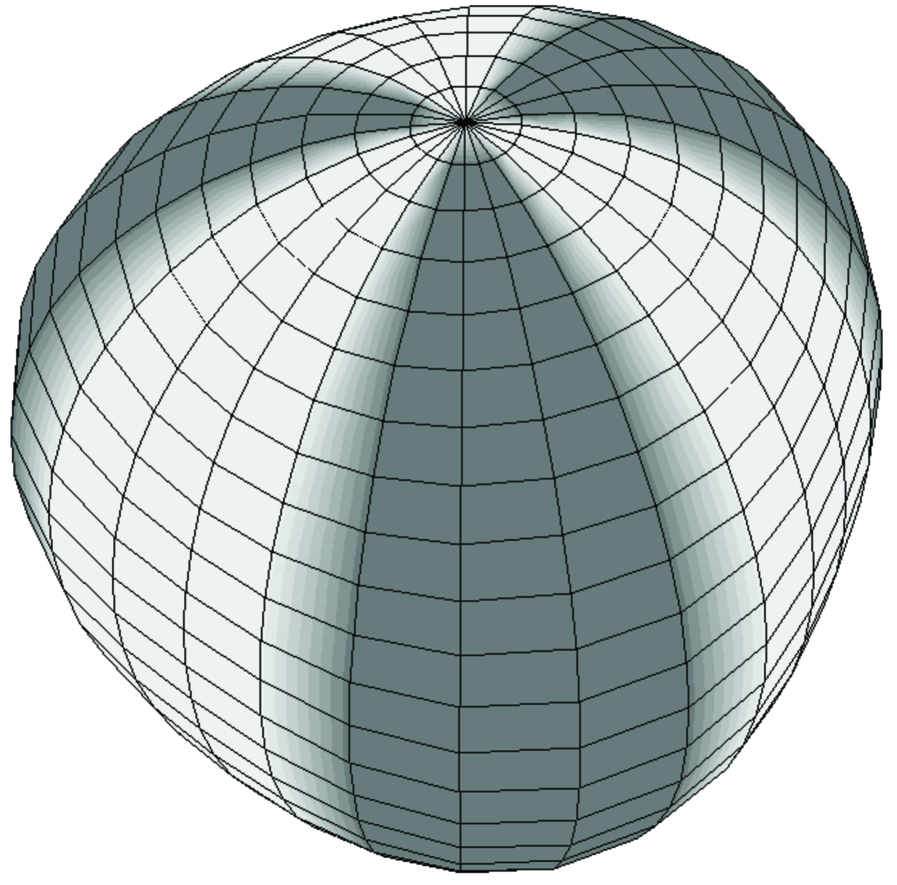
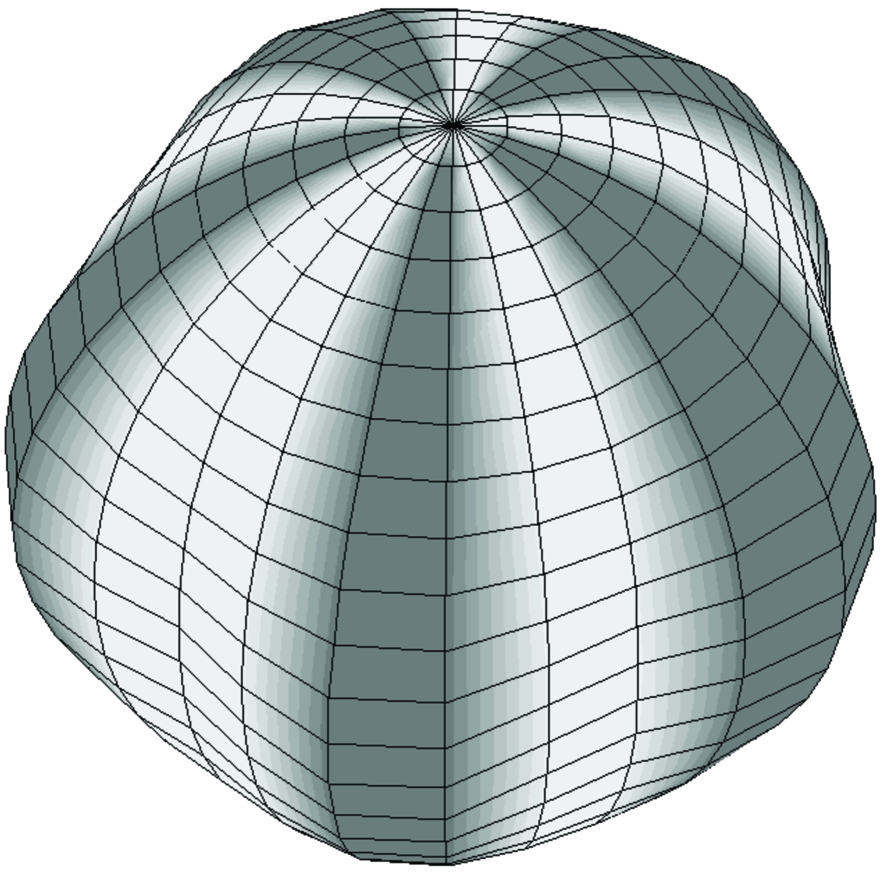
$n=3$ $k=3$	$n=5$ $k=5$
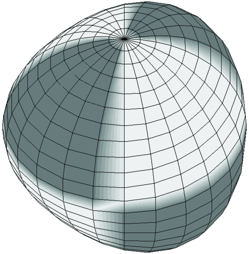
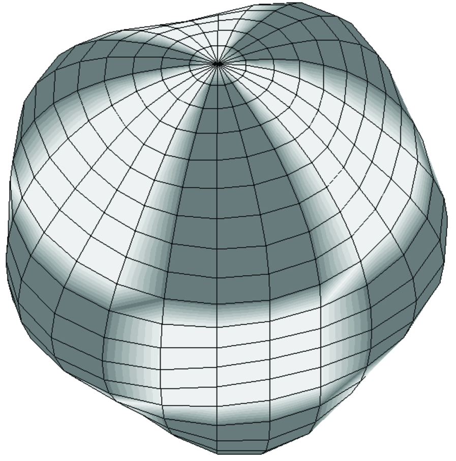
$n=3$ $k=2$	$n=5$ $k=3$

Figure 6.6: Real parts of spherical functions $Y_{nk}$ for several sets of $n$ and $k$ plotted on a sphere. The character of the functions is shown using the color code: dark gray corresponds to the areas where $Y_{nk}$ is positive, light gray is used where $Y_{nk}$ is negative.

Chapter 7 Satellite Motion

7.1 Typical perturbations in satellite motion

Summary: Non-sphericity of the gravitational field of the Earth. Gravitational forces of the Moon and the Sun. Planetary perturbations. Atmospheric drag. Light pressure. Magnetic field of the Earth. Neutral and charged particles. Relativistic perturbations.

It is obvious that nowadays the task to model the motion of Earth satellites plays an important role and even influences our every-day life. It is sufficient to mention communication satellites as well as the GPS, GLONASS and Galileo satellites. Also for scientific work Earth satellites play important role. It is well known, for example, that the analysis of the motion of specially designed satellites (LAGEOS, CHAMP, GRACE, GOCE, etc.) is the best way to measure the gravitational field of the Earth.

If the Earth were spherically symmetric, had no atmosphere and were the only massive body in the universe, the orbit of a satellite in the framework of Newtonian physics would be one of the solutions of the two-body problem discussed in Chapter 2. None of these conditions is met in reality. An orbit that would be an ellipse in the ideal case, is still close to an ellipse in real world. However, several sorts of perturbations lead to time-dependent osculating elements of the orbit. Which perturbations have to be taken into account to describe the motion of a satellite depends both on the parameters of the orbit and on the required accuracy. The main perturbations that must be taken into account for most satellites are:

• the effects of the deviation of the Earth’s gravity from spherical symmetry as described by coefficients $J_{n}$, $\overline{C}_{nk}$ and $\overline{S}_{nk}$ in (6.60);

• air drag caused by the motion of the satellite through the rarefied upper atmosphere;

• $N$-body perturbations due to the Moon and the Sun.

The first perturbation in this list is the largest one for asteroids flying at the altitudes between approximately 300 and 30000 km above the surface of the Earth. Air drag is the largest perturbation for lower satellites (whose with the altitudes lower than about 300 km). For higher flying satellites (altitude over about 30000 km) the $N$-body perturbations from the Moon and the Sun are the most important ones.

For high accuracy modelling (mostly important for scientific satellites of various kinds) more subtle effects should be taken into account:

• the effects of the tidal deformations of the gravitational field (tidally induced temporal variations of $J_{n}$, $\overline{C}_{nk}$ and $\overline{S}_{nk}$); both solid tides and ocean tides should be taken into account here;

• $N$-body perturbations due to other bodies of the Solar system (mostly due to Jupiter and Venus)

• light pressure from the light from the Sun and reflected light from the Earth; the effects of umbra (shadow) and penumbra (the part of a shadow where the light source is only partially blocked) should be taken into account; the “light” should be considered not only in the “visual band”, but also in other wavebands (especially, infrared);

• effects of the general theory of relativity;

• effects of the magnetic field of the Earth;

• effects of cosmic particles (both neutral and charged ones).

Several perturbations mentioned above (e.g., light pressure and magnetic field) require to model simultaneously also the dynamics of the attitude (spatial orientation) of the satellite. In general, high-accuracy modelling of satellite motion is a truly complicated task. In this Chapter we will discuss only two sorts of perturbations in their simplest form: the perturbations due to the oblateness of the Earth and those due to the atmospheric drag.

7.2 Motion in the quadrupole field

Summary: The disturbing function for the oblate Earth. Solution in osculating elements. Secular perturbations. Numerical example. Periodical perturbations.

For the Earth (and all major planets of the solar system) the second zonal harmonic $J_{2}$ is significantly larger than all other coefficients in the expansion (6.60) of the gravitational potential. Indeed, for the Earth $J_{2}\approx 1.083\times 10^{-3}$ while other coefficients are of the order of $10^{-6}$. For Earth satellites with the altitudes between about 300 and 30000 km the effects of $J_{2}$ is the largest perturbation effect. Let us consider it in more detail.

7.2.1 Disturbing potential due to $J_{2}$

Let us neglect all other terms in (6.60) and write the gravitational potential of the Earth as

$$U={GM\over r}\left(1-J_{2}\,{R^{2}\over r^{2}}\,P_{2}(\sin\varphi)\right),$$ (7.1)

where $\varphi=\displaystyle{\pi\over 2}-\theta$ is the geographic latitude, $R$ is now the equatorial radius of the Earth ($R\approx 6378\,{\rm km}$), and $M$ is the mass of the Earth ($GM\approx 3.986004\times 10^{14}\,{\rm m}^{3}/{\rm s}^{2}$). The gravitational potential does not explicitly depend on time (we assume $J_{2}={\rm const}$) and does not depend on the longitude $\lambda$. The latter circumstance is related to the fact that if we only consider $J_{2}$ the gravitational field is axially symmetric (see Section 6.3.1 above). The gravitational potential $U$ is considered now as a function of coordinates $r$ and $\varphi$. The potential (7.1) can be written as

$$U = {G\,M\over r}+{\cal R}\,,$$ (7.2)

$${\cal R} = -{G\,M\over r}\,J_{2}\,{R^{2}\over r^{2}}\,P_{2}(\sin\varphi),$$ (7.3)

where ${\cal R}$ can be considered as a perturbation of the two-body motion with potential ${GM\over r}$. Then the equations of motion of the satellite are given by (3.13) with $m_{0}=0$ (the influence of the satellite on the motion of the Earth is neglected) and with gradient of ${\cal R}$ on the right-hand side.

The analysis of the motion can be done using the Lagrange equations discussed in Section 4.3. In order to use those equations we have to express ${\cal R}$ as function of orbital elements. Position ${\mbox{\boldmath$r$}}=(x,y,z)$ of the satellite can be described using its geocentric distance $r$ and geographical longitude $\lambda$ and latitude $\varphi$ as

$$\pmatrix{x\cr y\cr z}=\pmatrix{r\,\cos\lambda\,\cos\varphi\cr r\,\sin\lambda\,\cos\varphi\cr r\,\sin\varphi}\,.$$

Using (2.28), (2.33) and (2.45)–(2.46) one gets

$$\sin\varphi={z\over r}=\sin i\,\sin(v+\omega),$$ (7.4)

where $i$ is the inclination of the orbit, $\omega$ is the argument of geocenter and $v$ is the true anomaly. Therefore, one gets

$$P_{2}(\sin\varphi)={3\over 2}\,\sin^{2}i\,\sin^{2}(v+\omega)-{1\over 2}={3\,\sin^{2}i-2\over 4}-{3\over 4}\,\sin^{2}i\,\cos 2(v+\omega)\,.$$ (7.5)

The disturbing potential can than be written as

$${\cal R} = {\mu\over a^{3}}\,{a^{3}\over r^{3}}\,\left({3\,\sin^{2}i-2\over 4}-{3\over 4}\,\sin^{2}i\,\cos 2(v+\omega)\right)\,,$$ (7.6)

$$\mu = J_{2}\,G\,M\,R^{2},$$ (7.7)

where $a$ is the semi-major axis or the orbit.

7.2.2 Exact consequence of the axially symmetric perturbation

Since

$${a\over r}={1+e\,\cos v\over 1-e^{2}},$$

$e$ being the eccentricity, and the true anomaly is a function of the mean anomaly $M$ and the eccentricity $e$ only, one can see that the disturbing potential ${\cal R}$ depends on $a$, $e$, $i$, $\omega$ and $M$, but does not depend on the longitude of the node $\Omega$. This is again the consequence of the fact that the assumed model for the Earth gravity is axially symmetric. Indeed, the only effect of a change of $\Omega$ is a rotation of the orbit as a whole with respect to the z-axis (see Fig. 2.3), but, in our model, the gravitational force does not depend on such a rotation. One can demonstrate that if ${\cal R}\neq{\cal R}(\Omega)$ the following combination of osculating elements remains constant:

$$\sqrt{a\,(1-e^{2})}\,\cos i={\rm const}\,.$$ (7.8)

Exercise. Demonstrate that

$${d\over dt}\,\left(\sqrt{a\,(1-e^{2})}\,\cos i\right)={1\over\kappa}\,{\partial R\over\partial\Omega}\,,$$ (7.9)

where $\kappa^{2}=n^{2}\,a^{3}$, $n$ being the mean motion. Hint: use the Lagrange equations (4.41)–(4.43).

This means that as soon as the disturbing potential is axially symmetric, the combination $\sqrt{a\,(1-e^{2})}\,\cos i$ remains constant.

7.2.3 Secular part of the disturbing potential

Now, let us confine our discussion to secular changes of the osculating elements, that is to the changes that polynomially depend on time. To this end let us consider the Fourier expansion of ${\cal R}$ in multiples of the mean anomaly $M$:

$${\cal R}={\cal R}_{0}+\sum_{k=1}^{\infty}\left({\cal R}_{k}\cos kM+\widetilde{\cal R}_{k}\sin kM\right)\,,$$ (7.10)

where ${\cal R}_{k}={\cal R}_{k}(a,e,i,\omega)$ for $k\geq 0$. We are only interested in the effect of ${\cal R}_{0}$.

Let us calculate the Fourier expansion of (7.6). Two functions should be expanded: $\displaystyle{a^{3}\over r^{3}}$ and $\displaystyle{a^{3}\over r^{3}}\,\cos 2(v+\omega)$. Eq. (2.90) allows one to write

$${a^{3}\over r^{3}} = \sum_{k=-\infty}^{\infty}X^{-3,0}_{k}(e)\,\cos kM=X^{-3,0}_{0}(e)+\sum_{k=1}^{\infty}2\,X^{-3,0}_{k}(e)\,\cos kM.$$ (7.11)

The first equality uses the fact that the Hansen coefficients $X^{n,m}_{k}$ are real and, therefore, the real parts and imaginary parts of (2.90) also hold:

$$\left({r\over a}\right)^{n}\,\cos m\,v = \sum_{k=-\infty}^{\infty}X_{k}^{n,m}(e)\,\cos k\,M\,,$$ (7.12)

$$\left({r\over a}\right)^{n}\,\sin m\,v = \sum_{k=-\infty}^{\infty}X_{k}^{n,m}(e)\,\sin k\,M\,.$$ (7.13)

For the second equality in (7.11) we use the well-known general symmetry property of the Hansen coefficients

$$X^{n,m}_{k}=X^{n,-m}_{-k}.$$ (7.14)

Indeed, the substitution $m\to-m$, $k\to-k$ and $\buildrel\circ\over{\hbox{\rm\char 16\relax}}\to-\buildrel\circ\over{\hbox{\rm\char 16\relax}}$ in (2.90) changes nothing and demonstrate (7.14). For $m=0$ as in (7.11) one has $X^{n,0}_{-k}=X^{n,0}_{k}$ so that each term with $k<0$ can be written together with the corresponding term with $k>0$. This leads to (7.11).

On the other hand, using (2.90) for $n=-3$ and $m=2$ ($\buildrel\circ\over{\hbox{\rm\char 16\relax}}$ being the imaginary unit, $\buildrel\circ\over{\hbox{\rm\char 16\relax}}^{2}=-1$)

$$\left({a\over r}\right)^{3}\,e^{\buildrel\circ\over{\hbox{\rm\char 16\relax}}\,2\,v} = \sum_{k=-\infty}^{\infty}X_{k}^{-3,2}(e)\,e^{\buildrel\circ\over{\hbox{\rm\char 16\relax}}\,k\,M}\,,$$ (7.15)

one can write

$$\left({a\over r}\right)^{3}\,e^{\buildrel\circ\over{\hbox{\rm\char 16\relax}}\,2\,v}\,e^{\buildrel\circ\over{\hbox{\rm\char 16\relax}}\,2\,\omega}\, = \sum_{k=-\infty}^{\infty}X_{k}^{-3,2}(e)\,e^{\buildrel\circ\over{\hbox{\rm\char 16\relax}}\,k\,M}\,e^{\buildrel\circ\over{\hbox{\rm\char 16\relax}}\,2\,\omega}\,,$$ (7.16)

or

$$\left({a\over r}\right)^{3}\,e^{\buildrel\circ\over{\hbox{\rm\char 16\relax}}\,2\,(v+\omega)}\, = \sum_{k=-\infty}^{\infty}X_{k}^{-3,2}(e)\,e^{\buildrel\circ\over{\hbox{\rm\char 16\relax}}\,(kM+2\omega)}$$ (7.17)

and, finally,

$$\left({a\over r}\right)^{3}\,\cos 2(v+\omega)\, = \sum_{k=-\infty}^{\infty}X_{k}^{-3,2}(e)\,\cos(kM+2\omega)$$ (7.18)

$$= X_{0}^{-3,2}(e)\,\cos 2\omega+\sum_{k\neq 0}X_{k}^{-3,2}(e)\,\cos(kM+2\omega)\,.$$

This means that

$${\cal R}_{0}={\mu\over a^{3}}\,\left({3\,\sin^{2}i-2\over 4}\,X^{-3,0}_{0}-{3\over 4}\,\sin^{2}i\,X^{-3,2}_{0}\,\cos 2\omega\right)\,.$$ (7.19)

The Hansen coefficients $X_{k}^{n,m}(e)$ can be computed in a variety of ways (see, e.g. Giacaglia, 1976). One possible (but, generally speaking, inefficient) way is to compute the Hansen coefficients from their definition as a Fourier coefficient:

$$X^{n,m}_{k}={1\over 2\pi}\,\int_{0}^{2\pi}{\left({1-e^{2}\over 1+e\cos v}\right)}^{n}\,\cos(m\,v-k\,M)\,dM\,.$$ (7.20)

For $k=0$ it is sufficient to use (2.35) to replace $dM$ by $dv$ as

$$dM={\left(1-e^{2}\right)^{3/2}\over(1+e\,\cos v)^{2}}\,dv$$ (7.21)

to get

$$X^{n,m}_{0}={1\over 2\pi}\,\left(1-e^{2}\right)^{n+3/2}\,\int_{0}^{2\pi}{\cos m\,v\over{\left({1+e\cos v}\right)}^{n+2}}\,dv\,.$$ (7.22)

Computing this integral for $n=-3$, and $m=0$ and $m=2$ is trivial and one gets

$$X^{-3,0}_{0} = (1-e^{2})^{-3/2}\,,$$ (7.23)

$$X^{-3,2}_{0} = 0\,.$$ (7.24)

With these expressions for the required Hansen coefficients one, finally, gets

$${\cal R}_{0}={\mu\over a^{3}}\,{3\,\sin^{2}i-2\over 4}\,(1-e^{2})^{-3/2}\,.$$ (7.25)

7.2.4 Secular perturbations of osculating elements

Since ${\cal R}_{0}$ depends only on $a$, $e$ and $i$, one has

$${\partial{\cal R}_{0}\over\partial\overline{M}_{0}}={\partial{\cal R}_{0}\over\partial\omega}={\partial{\cal R}_{0}\over\partial\Omega}=0\,.$$

The Lagrange equations (4.41)–(4.43) give in this case

$$a^{(0)}={\rm const}\,,$$ (7.26)

$$e^{(0)}={\rm const}\,,$$ (7.27)

$$i^{(0)}={\rm const}\,.$$ (7.28)

This means that the semi-major axis $a$, eccentricity $e$ and inclination $i$ remain constant. Index ’$(0)$’ in (7.26)–(7.28) and in equations for $\omega$, $\Omega$ and $\overline{M}_{0}$ below stresses that the equations are valid only in the approximation ${\cal R}={\cal R}_{0}$.

The partial derivatives of (7.25) read

$${\partial{\cal R}_{0}\over\partial a} = -\mu\,{3\,(2-3\,\sin^{2}i)\over 4\,a^{4}}\,{\left(1-e^{2}\right)}^{-3/2}\,,$$ (7.29)

$${\partial{\cal R}_{0}\over\partial e} = \ \mu\,{3\,e\,(2-3\,\sin^{2}i)\over 4\,a^{3}}\,{\left(1-e^{2}\right)}^{-5/2}\,,$$ (7.30)

$${\partial{\cal R}_{0}\over\partial i} = -\mu\,{3\,\sin i\,\cos i\over 2\,a^{3}}\,{\left(1-e^{2}\right)}^{-3/2}\,.$$ (7.31)

Substituting these partial derivatives in the Lagrange equations (4.44)–(4.46) and considering that semi-major axis $a$, eccentricity $e$ and inclination $i$ remain constant according to (7.26)–(7.28) one get the following simple solution for other three osculating elements:

$$\omega^{(0)}(t) = n_{\omega}\,(t-t_{0})+\omega^{(0)}(t_{0})\,,$$ (7.32)

$$\Omega^{(0)}(t) = n_{\Omega}\,(t-t_{0})+\Omega^{(0)}(t_{0})\,,$$ (7.33)

$$\overline{M}_{0}^{(0)}(t) = n_{\overline{M}_{0}}\,(t-t_{0})+\overline{M}_{0}^{(0)}(t_{0})\,,$$ (7.34)

where the drift rates read

$$n_{\omega} = {3\mu\,(4-5\,\sin^{2}i)\over 4\,\kappa\,a^{7/2}{(1-e^{2})}^{2}}\,,$$ (7.35)

$$n_{\Omega} = -{3\mu\,\cos i\over 2\,\kappa\,a^{7/2}{(1-e^{2})}^{2}}\,,$$ (7.36)

$$n_{\overline{M}_{0}} = {3\mu\,(2-3\,\sin^{2}i)\over 4\,\kappa\,a^{7/2}{(1-e^{2})}^{3/2}}\,.$$ (7.37)

Thus, in the general case the averaged elliptical orbit of a satellite in the field of oblate Earth characterized by $J_{2}$ is an ellipse that (a) linearly precesses around the $z$-axis (linear change of $\Omega$), (b) linearly precesses in the orbital plane (linear change of $\omega$), and (c) has the period different by a constant from $P={2\pi\over n}$, $n=\kappa\,a^{-3/2}$ (linear change in $\overline{M}_{0}$).

7.2.5 Analysis of the secular perturbations

Let us give a numerical value for the drifts for a particular satellite (we recall that $\kappa=\sqrt{GM}$ and $\mu$ is defined by (7.7)):

$$\left\{\begin{array}[]{ccl}a&=&12000\ {\rm km}\\ i&=&20^{\circ}\\ e&=&0.1\end{array}\right.\Longrightarrow\left\{\begin{array}[]{ccl}n_{\omega}&=&\phantom{-}1.9^{\circ}/{\rm day}\\ n_{\Omega}&=&-1.4^{\circ}/{\rm day}\\ n_{\overline{M}_{0}}&=&\phantom{-}0.9^{\circ}/{\rm day}\end{array}\right.\,.$$ (7.38)

This demonstrates that the effects are significant even for relatively high satellites ($a=12000\ {\rm km}$, $e=0.1$ corresponds to the altitude of about 4500 km in the perigee).

From (7.35)–(7.37) one can see that choosing some specific inclinations $i$ each of the drifts (7.35)–(7.37) can be made zero. Indeed,

• For $i=90^{\circ}$ one has no rotation of the orbital plane $n_{\Omega}=0$. The orbits with $i=90^{\circ}$ go straightly over the poles of the Earth and are called polar orbits. These orbits are used e.g., for special scientific satellites that have to observe some objects fixed in space. For example, the mission GP-B (Gravity Probe B) aimed at high-accuracy testing of general relativity, the future astrometric mission J-MAPS (Joint Milli-Arcsecond Pathfinder Survey) of the US Naval Observatory and the mission GRACE to monitor the gravity field of the Earth all use such polar orbits. The argument of perigee still changes for such orbits. Fig. 7.1 illustrates the form of the orbit in the orbital plane.

• For $i=\arcsin\displaystyle{2\over\sqrt{5}}\approx 63^{\circ}26^{\prime}5.82^{\prime\prime}$ and $i=\pi-\arcsin\displaystyle{2\over\sqrt{5}}\approx 116^{\circ}33^{\prime}54.18^{\prime\prime}$ the perigee $\omega$ does not precess since $n_{\omega}=0$. The orbits with such inclinations are used e.g. for special communication satellites especially useful for polar regions.

  Indeed, usual communication or broadcasting satellites are placed on the so-called geostationary orbit. Geostationary orbit is a circular orbit ($e=0$) with inclination $i=0$ (orbital plane of the satellite coincides with the equatorial plane of the Earth) and semi-major axis $a=42164\ {\rm km}$ chosen in such a way that the orbital period of the satellite exactly coincides with the rotational period of the Earth. From the point of view of an observer on the surface of the Earth a geostationary satellite is “seen” at a fixed position on the sky. This allows the observer to orient his communication antennas only once. The altitude of a geostationary satellite over the horizon is $90^{\circ}-|\varphi|$, where $\varphi$ is the geographical latitude of the observer. If the observer is situated in polar regions with $|\varphi|>70^{\circ}$ the geostationary satellites are “seen” too low over the horizon. This would require significant power increase to guarantee reliable communications.

  Already since the middle of 1960s a series of Soviet/Russian Molniya (Russian: “Lightning”) communications satellites for polar regions used a different principle. Molniya satellites have orbits with inclination $i\approx 63^{\circ}26^{\prime}$, high eccentricity $e\approx 0.722$ and periods of 12 hours. Such an orbit is often called Molniya orbit. Because of high eccentricity the satellite spend most of time far away from the Earth moving relatively slowly with respect to the Earth surface. As a result one such satellite provides communication and broadcasting services for about 8 hours per day. Three such satellites are sufficient to make the service available at each moment of time.

  Fig. 7.2 illustrates the form of the orbit with precessing $\Omega$.

• Finally, for $i=\arcsin\displaystyle{\sqrt{2\over 3}}\approx 54^{\circ}44^{\prime}8.20^{\prime\prime}$ and $i=\pi-\arcsin\displaystyle{2\over\sqrt{5}}\approx 125^{\circ}15^{\prime}51.80^{\prime\prime}$ the orbital period of the satellite is given by the unperturbed two-body relations $P={2\pi\over n}$, $n=\kappa\,a^{-3/2}$ since $n_{\overline{M}_{0}}=0$. No practical applications of such orbits are known.

7.2.6 Additional remarks

The problem of motion in the gravitational field of $J_{2}$ can be solved exactly without averaging. In addition to secular effects that were considered above one can consider all periodic terms in (7.10). In a more elegant way this can be done by considering the whole perturbation given by (7.6) and using simultaneously both true and mean anomalies in the resulting formulas. This allows one to derive the formulas for the first-order variations of osculating elements in closed form (see Roy, 2005, pp. 317–318). The first-order variations mean here that terms that are at least quadratic in $J_{2}$ are neglected.

The effects of other coefficients $J_{n}$, $n\geq 3$ as well as $\overline{C}_{nk}$ and $\overline{S}_{nk}$ in (6.60) can be analyzed in a similar way. One can show, for example, that the coefficients $J_{n}$ with odd $n$ lead only to periodic effects. For Lageos all coefficients with $n$ up to $n=50$ should be taken into account. The motion of missions like CHAMP, GRACE, GOCE, etc. is sensitive to the coefficients with much higher values of $n$. Thus, the data of CHAMP is sensitive to the coefficients with $n$ up to $n=140$, that of CRACE up to $n=180$ and GOCE up to $n=250$.

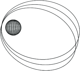
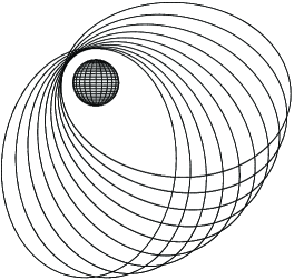
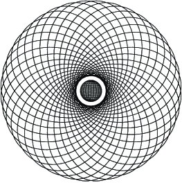
Figure 7.1: An orbit with precessing argument of pericenter $\omega$ is shown for 3, 10 and 36 periods of motion. The change of $\omega$ is taken to be $10^{\circ}$ per period.

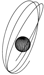
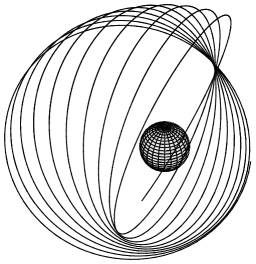
Figure 7.2: An orbit with precessing longitude of the node $\Omega$ is shown for 3, 10 and 36 periods of motion. The change of $\Omega$ is taken to be $10^{\circ}$ per period.

7.3 Atmospheric drag

Summary: The model of the perturbing force. Models for the atmospheric pressure. Gaussian perturbation equations for the atmospheric drag. Averaging of the equations. The simplified Gaussian perturbation equations for small eccentricities. Solution and its properties.

Let us now turn to the perturbations due to the atmospheric drag. Although the air in the upper atmosphere has very low density, it influences significantly the motion of satellites (recall that the velocity of satellites amounts to several km/s). For low satellites with altitude 300 km and less the atmospheric drag is the largest perturbation. Air drag can be understood as a result of friction between the air and the body of the satellite. As with all other friction forces the mechanical energy of the system does not remain constant, but is partially transformed into other sorts of energy (thermal one, etc.). It means that the air drag force does not have a potential and should be considered using the Gaussian perturbation equations (4.27)–(4.32). In general modelling of atmospheric drag is a very complex problem. Here we consider the simplest case. More detailed discussion can be found e.g. in King-Hele (1987).

7.3.1 Model for the drag force

We consider here the problem of motion of a body through a medium (fluid or gas). The relative velocity of this motion is denoted $v$. It is well known that for the case of small velocities $v=|{\mbox{\boldmath$v$}}|$ the flow of the media is laminar and the friction force is linearly proportional to $v$: $F_{S}\propto v$. This is called Stokes’ friction model (George Gabriel Stokes 1819–1903). For larger velocities $v$ the flow becomes turbulent and the drag force is described by the Newtonian friction model:

$$F_{N}={1\over 2}\,\rho\,C_{d}\,S\,v^{2},$$ (7.39)

where $\rho$ is the air density, $S$ is the area of the cross section of the body perpendicular to the direction of motion, $C_{d}$ is the numerical drag coefficient that depends on the geometry of the body (see Fig. 7.3 for a few examples).

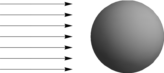
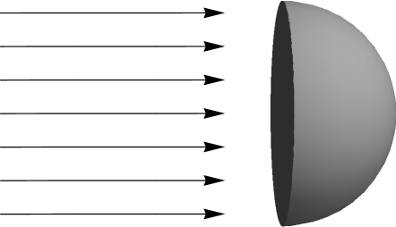
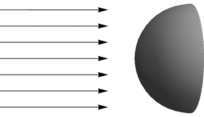
$C_{d}=0.4$	$C_{d}=1.3$	$C_{d}=0.3$

Figure 7.3: Drag coefficients for some bodies: a sphere and a half-sphere moving along its symmetry axis in two directions.

In reality the situation is more difficult. The effect of atmosphere results in several effects: (1) air drag force with a magnitude given by (7.39) and directed along $-{\mbox{\boldmath$v$}}$, (2) lift force directed perpendicular to $v$ (similar to the lift force for airplanes), (3) angular moment leading to a rotation of the body. We completely ignore the lift forces since they are important for higher densities of air when the motion in lower atmosphere is considered. As for the angular moment, we simply average the force (7.39) over several rotations of the satellite. Finally we get the disturbing force due to atmospheric drag in the form:

$${\mbox{\boldmath$F$}}=-C\,\rho\,v^{2}\,{{\mbox{\boldmath$v$}}\over v},$$ (7.40)

where $C={1\over 2}\,\overline{C}_{d}\,\overline{S}$, and an overline means averaging over the rotation of the satellite. We consider parameter $C$ to be known. Since velocity $v$ can be computed from the osculating elements of the orbit, the only unknown in (7.40) is the air density $\rho$.

7.3.2 Model for the air density

The air density can be taken from available models for the Earth’s atmosphere. These models are based both of theoretical modelling and on the results of measurements of various atmospheric parameters. The models are thus semi-empirical. Fig. 7.4 shows the air density as a function of the height for different conditions. We see that the air density $\rho$ at a given altitude $h$ depends on the time (it is higher during daytime and lower at night): at a given altitude the air density can be different by a factor 2–10 depending on the time of the day. It also depends on the level of solar activity (the higher is the solar activity the higher is the density): $\rho$ can be different by a factor 2–100 depending on the solar activity. There are also a number of smaller effects: (1) the atmosphere rotates, (2) $\rho$ depends not only on the height $h$, but, to a smaller degree, also on the geographical longitude $\lambda$ and the latitude $\phi$.

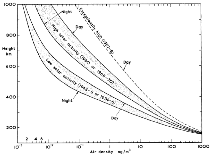
Figure 7.4: The density of air is shown as function of the altitude between 150 km and 1000 km for different conditions (day and night, low, high and exceptionally high solar activity). The plot is based on COSPAR International Reference Atmosphere 1972 (CIRA 1972).

Here we ignore all these complications and consider a simple model of exponential decay of the density:

$$\rho=A\,\exp\left(-{h\over H}\right),$$ (7.41)

where $\exp x\equiv e^{x}$, $h$ is the height over the Earth’s surface, $A=\rho(0)$ is the density at $h=0$, and $H$ is height scale (that is, the height difference for which the density decreases by a factor of $e=2.71\dots$). At the surface of the Earth $A\approx 1.3\ {\rm kg}/{\rm m}^{3}$ and $H\approx 8\ {\rm km}$. Such a model describes the air density quite well if the considered region of heights is sufficiently small. Density $\rho$ is shown on Fig. 7.4 in logarithmic scale. Therefore, the model (7.41) looks on Fig. 7.4 as a straight line. Clearly, model (7.41) can be used for a sequence of layers $h\in[h_{i},h_{i+1}]$, $i=1,\dots,K$ with some boundaries $h_{i}$ and with constants $A=A_{i}$ and $H=H_{i}$ depending on the layer. Such a layered model means that the curves on Fig. 7.4 are approximated by a piecewise linear curve. This is always possible, and the thinner are the layers the better is the approximation. Thus, the height scale $H$ can be considered as function $h$. Both theoretical considerations and Fig. 7.4 demonstrate that $dH/dh>0$ that is, the density decreases slower than exponentially (slower than prescribed by (7.41)). In the following we simplify the model further and consider that the orbit lies within one layer of $h$ and the coefficients $A$ and $H$ in (7.41) are some given constants. Then we should express $\rho$ as function of osculating elements of the orbit. Considering that the radial distance of the satellite $r=R+h$ and, on the other side, $r=a(1-e\,\cos E)$, cf. Eq.(2.44), we can write

$$\rho = A\,\exp\left(-{h\over H}\right)=A\,\exp\left(-{r-R\over H}\right)=A\,\exp\left({R\over H}\right)\,\exp\left(-{r\over H}\right)$$ (7.42)

$$= A\,\exp\left({R\over H}\right)\,\exp\left(-{a-a\,e\,\cos E\over H}\right)=A\,\exp\left(-{a-R\over H}\right)\,\exp\left({a\,e\,\cos E\over H}\right)\,.$$

Introducing

$$B=A\,\exp\left(-{a-R\over H}\right)$$ (7.43)

one finally gets

$$\rho = B\,\exp\left({\mu\,\cos E}\right)\,,$$ (7.44)

$$\mu = {a\,e\over H}\,.$$ (7.45)

Note that $B$ has a simple meaning: $B$ is the air density $\rho$ at the height equal to $a-R$, i.e. at the mean altitude of the satellite. From the discussion above it is clear that this model works better for orbit with smaller eccentricities $e$. Below we will see that the air drag reduces the eccentricity $e$ of the orbit. Therefore, the model (7.44) for $\rho$ works better when one considers later stages of the orbital evolution.

7.3.3 Gaussian perturbation equations in the axes aligned with the velocity vector

We have seen above that the direction of the disturbing force is related to the direction of the orbital velocity $v$. On the other hand, the Gaussian perturbation equations (4.27)–(4.32) are expressed through the components $S$, $T$, and $W$ of the disturbing force $F$ as defined by (4.7)–(4.9). The components $(S,T,W)$ are immediately related to the vector $r$ of orbital position, $S$ being parallel to $r$. Let us introduce another coordinate system $(\tau,n,W)$ instead of $(S,T,W)$. Namely, let the axis $\tau$ be directly along the orbital velocity $v$ and the axis $n$ perpendicular to $\tau$ in the instantaneous orbital plane given by the vectors of orbital position $r$ and velocity $\dot{{\mbox{\boldmath$r$}}}={\mbox{\boldmath$v$}}$. Let $F_{\tau}$ and $F_{n}$ be components of $F$ in the axes $\tau$ and $n$, respectively. One can write:

$$F_{\tau} = {\dot{{\mbox{\boldmath$r$}}}\over|\dot{{\mbox{\boldmath$r$}}}|}\cdot{\mbox{\boldmath$F$}},$$ (7.46)

$$F_{n} = {\left({\mbox{\boldmath$r$}}\times\dot{{\mbox{\boldmath$r$}}}\right)\times\dot{{\mbox{\boldmath$r$}}}\over\left|{\mbox{\boldmath$r$}}\times\dot{{\mbox{\boldmath$r$}}}\right|\,|\dot{{\mbox{\boldmath$r$}}}|}\cdot{\mbox{\boldmath$F$}}.$$ (7.47)

Our goal is now to express the components $S$ and $T$ of $F$ as given by (4.7)–(4.8) in terms of $F_{\tau}$ and $F_{n}$. The relation between the axes is shown on Fig. 7.5. It is clear from the Figure that the components $(S,T)$ can be derived from $(F_{\tau},F_{n})$ by a rotation in the orbital plane by the angle $-\alpha$, $\alpha$ being the angle between vectors $r$ and $\dot{{\mbox{\boldmath$r$}}}$. It means

$$S = F_{\tau}\,\cos\alpha-F_{n}\,\sin\alpha\,,$$

$$T = F_{\tau}\,\sin\alpha+F_{n}\,\cos\alpha\,.$$ (7.48)

where $\cos\alpha$ and $\sin\alpha$ are defined as

$$\cos\alpha = {\dot{{\mbox{\boldmath$r$}}}\cdot{\mbox{\boldmath$r$}}\over|\dot{{\mbox{\boldmath$r$}}}|\,|{\mbox{\boldmath$r$}}|}={e\,\sin E\over\sqrt{1-e^{2}\,\cos^{2}E}}\,,$$

$$\sin\alpha = {\dot{{\mbox{\boldmath$r$}}}\times{\mbox{\boldmath$r$}}\over|\dot{{\mbox{\boldmath$r$}}}|\,|{\mbox{\boldmath$r$}}|}={\sqrt{1-e^{2}}\over\sqrt{1-e^{2}\,\cos^{2}E}}\,.$$ (7.49)

Here we used (2.45)–(2.46) and (2.48)–(2.49) for the components of $r$ and $\dot{{\mbox{\boldmath$r$}}}$, respectively. Substituting this transformation into the Gaussian perturbation equations (4.27)–(4.32) one get a version of the latter with components $F_{\tau}$ and $F_{n}$:

$${d\over dt}\,a = {2\over n}\,\sqrt{1+e\,\cos E\over 1-e\,\cos E}\,F_{\tau}\,,$$ (7.50)

$${d\over dt}\,e = {2(1-e^{2})\,\cos E\over a\,n\,\sqrt{1-e^{2}\cos^{2}E}}\,F_{\tau}-{\sqrt{1-e^{2}}\,\sin E\over a\,n}\,\sqrt{1-e\,\cos E\over 1+e\,\cos E}\,F_{n}\,,$$ (7.51)

$${d\over dt}\,\omega = {2\over n\,a}\,{\sqrt{1-e^{2}}\over e}\,{\sin E\over\sqrt{1-e^{2}\,\cos^{2}E}}\,F_{\tau}+{\cos E+e\over a\,n\,e}\,\sqrt{1-e\,\cos E\over 1+e\,\cos E}\,F_{n}$$ (7.52)

$$-r\,\sin(v+\omega)\,\cot i\,\left({W\over\kappa\sqrt{p}}\right),$$

$${d\over dt}\,\overline{M}_{0} = -{2\over a\,n\,e}\,{(1-e^{3}\cos E)\,\sin E\over\sqrt{1-e^{2}\cos^{2}E}}\,F_{\tau}$$ (7.53)

$$-{\sqrt{1-e^{2}}\,(\cos E-e)\over a\,n\,e}\,\sqrt{1-e\,\cos E\over 1+e\,\cos E}\,F_{n}\,.$$

The equations (4.29) and (4.31) for $i$ and $\Omega$ remain unchanged.

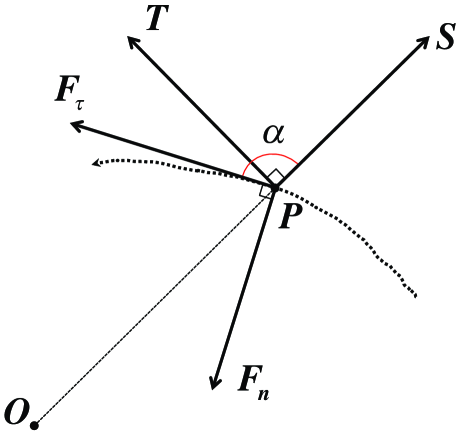
Figure 7.5: The plot shows the relation between the components of the perturbing force in two coordinate systems $(S,T)$ and $(F_{\tau},F_{n})$. Both systems are rectangular Cartesian ones so that the components are mutually orthogonal. Axis $S$ is directed parallel to the positional vector $r$ (from the origin $O$ to the current position $P$ of the body). Axis $\tau$ is directed along the instantaneous velocity of the body. The trajectory of the body is shown by a dotted curve and the arrow on that curve shows the direction of motion. Axis $\tau$ is tangential to the trajectory at a given moment of time. Finally, the angle between axes $S$ and $\tau$ is denoted by $\alpha$. Clearly, the relation between $(S,T)$ and $(F_{\tau},F_{n})$ is a simple rotation given by (7.3.3).

7.3.4 Osculating elements for the air drag

The disturbing force from the air drag is given by (7.40) and (7.44)–(7.45). The components of the disturbing force $F$ can be written as:

$$F_{\tau} = -C\,\rho\,v^{2}\,,$$ (7.54)

$$F_{n} = 0\,,$$ (7.55)

$$W = 0\,.$$ (7.56)

Therefore, the air drag does not change $i$ and $\Omega$, i.e. the orbital plane remains unchanged. In (7.50)–(7.53) only the terms proportional to $F_{\tau}$ should be considered. From (2.48)–(2.49) one gets

$$v^{2}=n^{2}\,a^{2}\,{1+e\,\cos E\over 1-e\,\cos E}.$$ (7.57)

Let us also change the left-hand side of (7.50)–(7.53) from the derivatives with respect to time $t$ to the corresponding derivatives with respect to the eccentric anomaly $E$. Using (2.47) for any element $\epsilon$ one has

$${d\epsilon\over dE} = {d\epsilon\over dt}\,\left({dE\over dt}\right)^{-1}={1-e\cos E\over n}\,{d\epsilon\over dt}.$$ (7.58)

In the following we are only interested in the form of the trajectory. Therefore, the element $\overline{M}_{0}$ plays no role and will be ignored below. Substituting (7.54) and (7.57) into (7.50)–(7.52) and using (7.58) for all elements one gets:

$${da\over dE} = -2a^{2}\,C\,\rho\,\sqrt{(1+e\,\cos E)^{3}\over 1-e\,\cos E},$$ (7.59)

$${de\over dE} = -2a\,C\,\rho\,(1-e^{2})\,\cos E\,\sqrt{1+e\,\cos E\over 1-e\,\cos E},$$ (7.60)

$${d\omega\over dE} = -2a\,C\,\rho\,e^{-1}\,\left(1-e^{2}\right)^{1/2}\,\sin E\,\sqrt{1+e\,\cos E\over 1-e\,\cos E}.$$ (7.61)

Now we can substitute the density model (7.44)–(7.45) and get

$${da\over dE} = -2a^{2}\,C\,B\,\exp\left(\mu\,\cos E\right)\,\sqrt{(1+e\,\cos E)^{3}\over 1-e\,\cos E},$$ (7.62)

$${de\over dE} = -2a\,C\,B\,(1-e^{2})\,\exp\left(\mu\,\cos E\right)\,\cos E\,\sqrt{1+e\,\cos E\over 1-e\,\cos E},$$ (7.63)

$${d\omega\over dE} = -2a\,C\,B\,e^{-1}\,\left(1-e^{2}\right)^{1/2}\,\sin E\,\exp\left(\mu\,\cos E\right)\,\sqrt{1+e\,\cos E\over 1-e\,\cos E}.$$ (7.64)

7.3.5 Averaged equations for the osculating elements

Let us investigate now only secular perturbations of $a$, $e$ and $\omega$. First, let us calculate the mean value of the derivatives of these three elements over a period of motion as

$$\left[{d\epsilon\over dE}\right]={1\over 2\,\pi}\,\int_{0}^{2\pi}{d\epsilon\over dE}\,dE={1\over 2\,\pi}\,\int_{-\pi}^{\pi}{d\epsilon\over dE}\,dE,$$ (7.65)

where again $\epsilon$ is any of the elements. Since $d\omega/dE$ given by (7.64) is an odd function of $E$ one has

$$\left[{d\omega\over dE}\right]=0\,.$$ (7.66)

This means that the osculating argument of perigee does not have secular variations, but only periodic ones. For the other two elements one gets

$$\left[{da\over dE}\right] = -{a^{2}\,C\,B\over\pi}\,\int_{0}^{2\pi}\exp\left(\mu\,\cos E\right)\,\sqrt{(1+e\,\cos E)^{3}\over 1-e\,\cos E}\,dE\,,$$ (7.67)

$$\left[{de\over dE}\right] = -{a\,C\,B\over\pi}\,(1-e^{2})\,\int_{0}^{2\pi}\exp\left(\mu\,\cos E\right)\,\cos E\,\sqrt{1+e\,\cos E\over 1-e\,\cos E}\,dE\,.$$ (7.68)

7.3.6 Averaged osculating elements for small eccentricities

At this point we need one more sort of special functions. Namely, $I_{m}(x)$ defined as

$$I_{m}(x)={1\over 2\pi}\int_{0}^{2\pi}\exp(\mu\,\cos E)\,\cos mE\,dE$$ (7.69)

are called modified Bessel functions of the first kind (sometimes hyperbolic Bessel functions of the first kind). Many properties of these functions are known (see Abramowitz & Stegun (1965), Chapter 9). They are related to the Bessel functions of the first kind given by (2.87) as

$$I_{m}(x)=\buildrel\circ\over{\hbox{\rm\char 16\relax}}^{-m}J_{m}(\buildrel\circ\over{\hbox{\rm\char 16\relax}}x),$$ (7.70)

and can be calculated through the following power series

$$I_{m}(x)=\sum_{l=0}^{\infty}{1\over l!(l+m)!}\,{\left({1\over 2}\,x\right)}^{m+2l}.$$ (7.71)

Functions $I_{m}(x)$ are shown on Fig. 7.6 for a few values of $m$. Below it will be important that

• $I_{m}(0)\neq 0$ only for $m=0$ (one has $I_{0}(0)=1$);

• $I_{m}(x)\geq 0$ for any $m$ and $x\geq 0$;

• $dI_{m}(x)/dx\geq 0$ for any $m$ and $x\geq 0$.

These properties can be seen directly from (7.70).

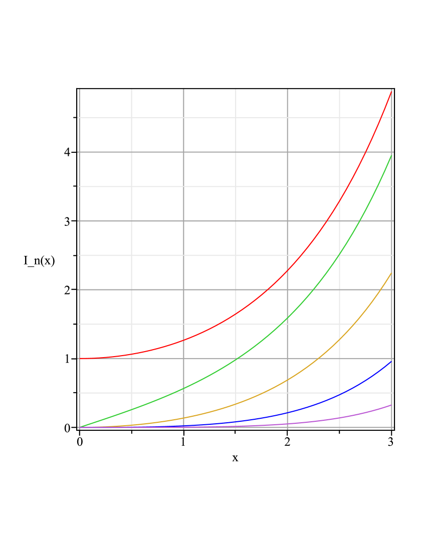
Figure 7.6: Modified Bessel functions of the first kind $I_{n}(x)$ are shown for $0\leq x\leq 3$ and $k=0$, $1$, $2$ and $3$ (red, green, yellow, blue, magenta).

Using $I_{m}(x)$ and considering the Taylor series

$$\sqrt{(1+e\,\cos E)^{3}\over 1-e\,\cos E} = 1+2\cos E\,e+{3\over 4}\,(1+\cos 2E)\,e^{2}+{\cal O}(e^{3})\,,$$ (7.72)

$$\cos E\,\sqrt{1+e\,\cos E\over 1-e\,\cos E} = \cos E+{1\over 2}(1+\cos 2E)\,e+{1\over 8}\left(3\cos E+\cos 3E\right)\,e^{2}+{\cal O}(e^{3})$$ (7.73)

one gets

$$\left[{da\over dE}\right] = -2a^{2}\,C\,B\,\left(I_{0}(\mu)+2e\,I_{1}(\mu)+{3\over 4}\,e^{2}\,\left(I_{0}(\mu)+I_{2}(\mu)\right)+{\cal O}(e^{3})\right)\,,$$ (7.74)

$$\left[{de\over dE}\right] = -2a\,C\,B\,(1-e^{2})\,\left(I_{1}(\mu)+{1\over 2}\,e\,\left(I_{0}(\mu)+I_{2}(\mu)\right)\right.$$ (7.75)

$$\phantom{-2a\,C\,B\,(1-e^{2})\,\biggl{(}\ }\left.+{1\over 8}\,e^{2}\,\left(3I_{1}(\mu)+I_{3}(\mu)\right)+{\cal O}(e^{3})\right)\,.$$

Here we expanded the equations in power of eccentricity $e$ and neglected terms of the order of $e^{3}$ and higher. It means that (7.74)-(7.75) are valid only for sufficiently small eccentricities. In principle, higher-order terms in $e$ can be calculated. However, for large $e$ it is better to solve (e.g., numerically) directly (7.67)-(7.68) or, directly, (7.62)-(7.64).

7.3.7 Discussion of the solution for osculating elements

Equations (7.74)-(7.75) are two differential equations for two unknown functions $a(E)$ and $e(E)$. These equations are coupled. Note also that $\mu$ depends on both $a$ and $e$ as given by (7.45). For a numerical example, the solution of (7.74)-(7.75) is shown on Fig. 7.7. Let us make several remarks.

• Since $I_{m}(\mu)\geq 0$ the right-hand sides of (7.74)-(7.75) are non-positive. It means that the averaged values of $a$ and $e$ are non-increasing function of $E$ (and, therefore, of time $t$). That is, both $a$ and $e$ becomes smaller during the evolution of the orbit.

• For circular orbits ($e=0$) the equations can be drastically simplified:

  $$\left[{da\over dE}\right] = -2a^{2}\,C\,B\,,$$ (7.76)

  $$\left[{de\over dE}\right] = 0\,.$$ (7.77)

  It means that the orbit remains circular with $e=0$ and that the semi-major axis decreases hyperbolically:

  $$a(E) = {1\over{1\over a(E_{0})}+2C\,B\,(E-E_{0})}\,,$$ (7.78)

  $a(E_{0})$, being an integration constant, is the value of $a$ for some initial moment $E=E_{0}$.

• The smaller becomes the eccentricity $e$, the smaller is the absolute value of the right-hand sides of (7.74)-(7.75). Here we used that ${dI_{m}(x)\over dx}\geq 0$ for any $n$ and $x\geq 0$. This means that the rate of change of both $a$ and $e$ decreases with time.

• Finally, let us note that because of the air drag, satellites become faster and not slower as one could expect from a friction force. This is of course related with the gravitational character of motion: if semi-major axes $a$ decreases, the velocity increases as $a^{-1/2}$. Indeed, Eq. (7.57) can be written as

  $$v=\sqrt{GM\over a}\,\sqrt{1+e\,\cos E\over 1-e\,\cos E}.$$ (7.79)

  Although the air drag as any friction force decreases the total mechanical energy of the system Earth-satellite, the potential energy $-GM/r$ of the system is transformed into the kinetic energy $v^{2}/2$ and the latter increases.

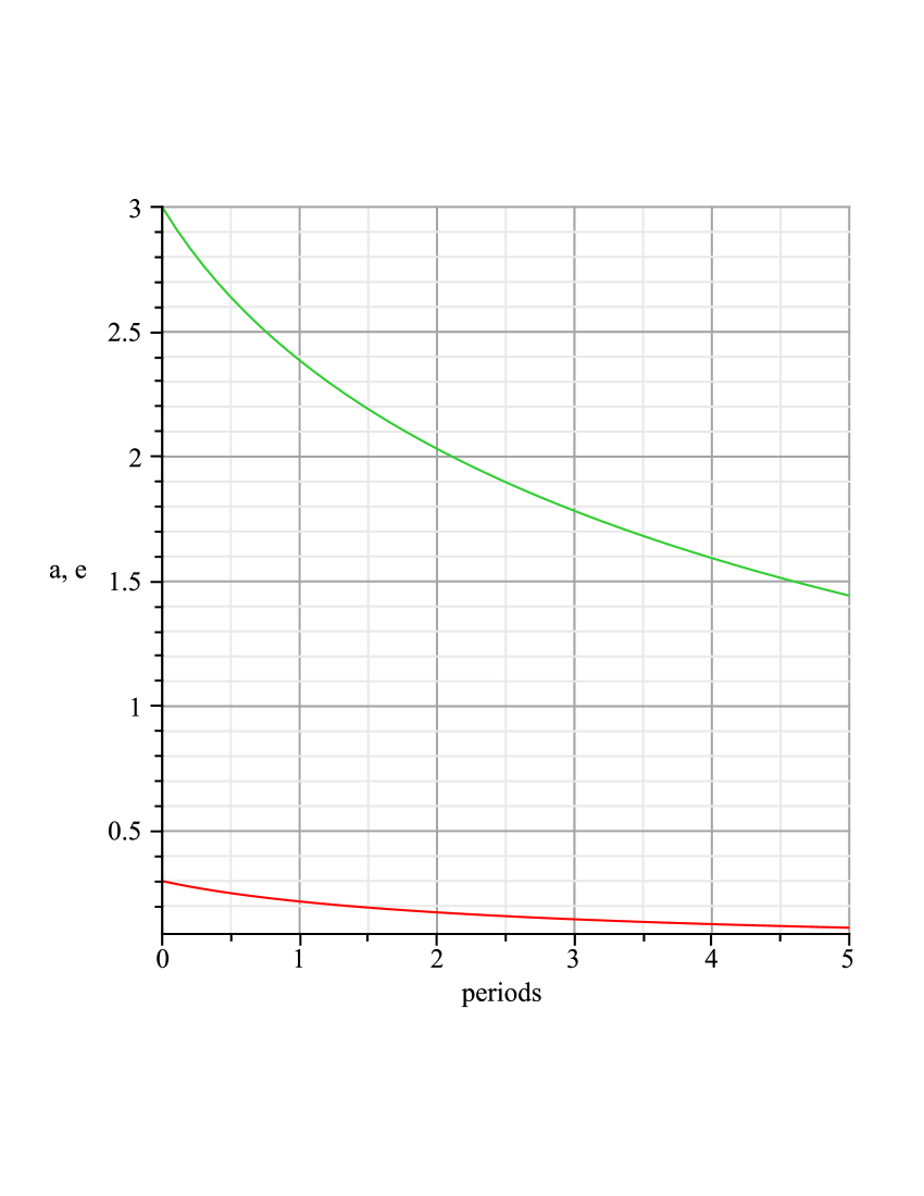
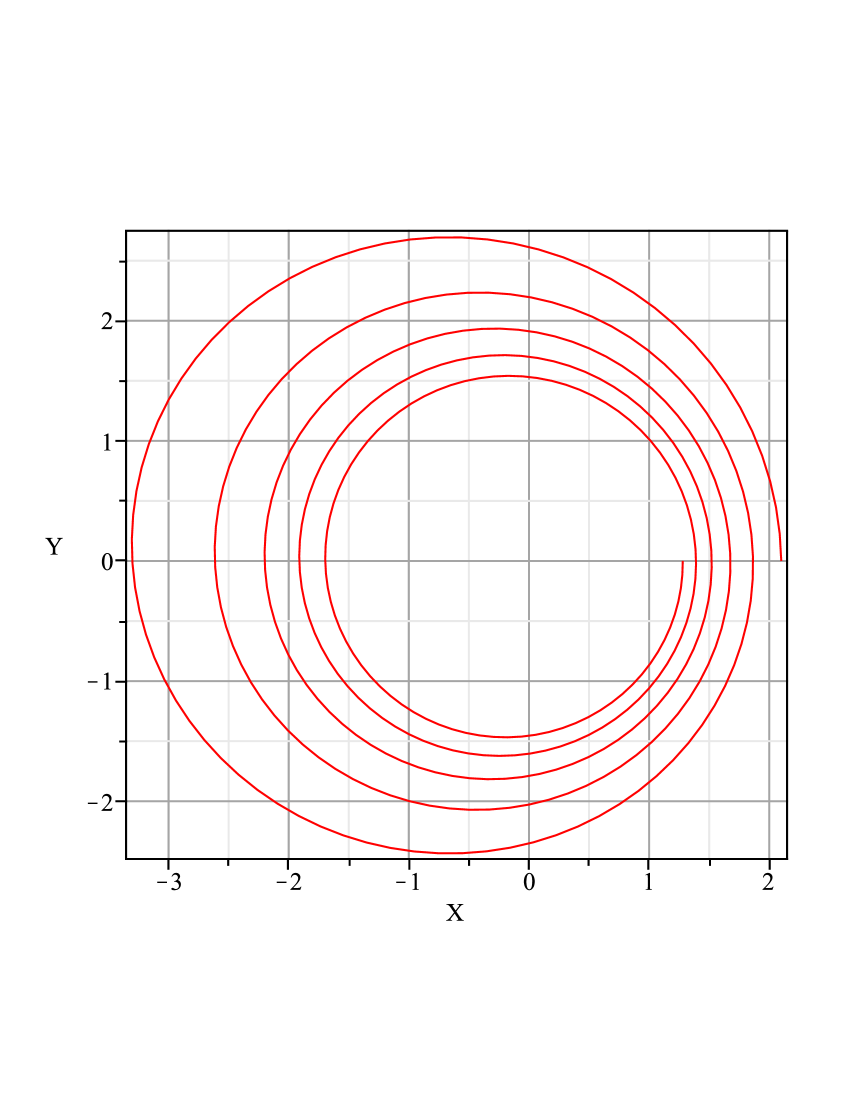
Figure 7.7: The left pane shows the variation of the osculating semi-major axes $a$ (upper green curve) and eccentricity $e$ (lower red curve) over several orbital periods. On the right pane the orbit of a satellite affected by the atmospheric drag is shown over the same interval of time. One can see that both the semi-major axis and the eccentricity decrease with time. The effect is exaggerated to make it better visible. Initial eccentricity is $e=0.3$.

Chapter 8 Numerical integration of ordinary differential equations

8.1 Basic notions

Summary: Euler step for the differential equations of the first order. Discretization. Three kinds of errors: the local truncation error, the global error and the roundoff error.

8.2 Methods of numerical integration

Summary: The method of Taylor expansion. The Runge-Kutta method. Stepsize control for the Runge-Kutta methods (Fehlberg method). The Runge-Kutta-Nyström method. Multistep methods. Explicit and implicit methods. Predictor-corrector methods. Adams-Bashforth and Adams-Moulton methods. Extrapolation methods.

8.3 Reliability of numerical integration

Summary: Close encounters. Regularization. Accuracy control.

Index

• aphel §2.3
• apoapsis §2.3
• apoastron §2.3
• apocenter §2.3
• apogee §2.3
• apse line §2.3
• apsides §2.3
• argument of latitude §4.2
• argument of pericenter §2.3
• ascending node §2.4
• associated Legendre polynomials §6.1.3
• Bessel functions of the first kind §2.9.2
• central configurations §2.1
• central forces §2.2
• disturbing function §3.3
• eccentricity §2.3
• Einstein-Infeld-Hoffmann equations §3.5
• Euler equations §4.2.2
• Gaussian perturbation equations §4.2.2
• geostationary orbit item -
• harmonic functions §6.1.1
• Hill’s surfaces of zero velocity §3.4
• hyperbolic Bessel functions of the first kind §7.3.6
• inclination §2.4
• integrals of motion §2.1
• invariant plane §3.2
• Jacobi integral §3.4
• Lagrange equations §4.3
• Lagrange solutions §3.4
• Laplace equation §6.1.1
• Laplace plane §3.2
• Legendre polynomials §6.1.2
• line of apsides §2.3
• Lissajous orbits §3.4
• longitude of the ascending node §2.4
• longitude of the node §2.4
• modified Bessel functions of the first kind §7.3.6
• Molniya orbit item -
• osculating elements §4.1
• periapsis §2.3
• periastron §2.3
• pericenter §2.3
• perigee §2.3
• perihelion §2.3
• polar orbits item -
• sectorial harmonics item 3.
• semi-latus rectum §2.3
• semi-major axis §2.3
• tesseral harmonics item 4.
• true anomaly §2.5
• variation of constants §4.1
• variation of parameters §4.1
• zonal harmonics item 2.

References

- (1)
- Aarseth (2003) Aarseth, S.J. 2003: Gravitational N-body Simulations: Tools and Algorithms (Cambridge: Cambridge University Press)
- Aarseth et al. (2008) Aarseth, S.J., Tout, Chr.A., Mardling, R.A. 2008: The Cambridge N-Body Lectures (Berlin: Springer)
- Abramowitz & Stegun (1965) Abramowitz, M., Stegun, I.A. 1965: Handbook of Mathematical Functions with Formulas, Graphs, and Mathematical Tables (New York: Dover)
- Arnold, Kozlov & Neishtadt (1997) Arnold, V.I., Kozlov, V.V., Neishtadt, A.I. 1997: Mathematical Aspects of Classical and Celestial Mechanics (Berlin: Springer)
- Beutler (2005) Beutler, G. 2005: Methods of Celestial Mechanics (Berlin: Springer)
- Bottke et al. (2006) Bottke, Jr., W.F., Vokrouhlický, D., Rubincam, D.P., Nesvorný, D. 2006: Annu. Rev. Earth Planet. Sci. 34, 157
- Bretagnon & Francou (1988) Bretagnon, P., Francou, G. 1988: Astron.Astrophys., 202, 309
- Brouwer & Clemence (1985) Brouwer, D., Clemence, G.M. 1985: Methods of Celestial Mechanics, 2nd impr. (Orlando: Academic Press)
- Chandrasekhar (1987) Chandrasekhar, S. 1987: Ellipsoidal Figures of Equilibrium (New York: Dover Publications)
- Chenciner & Montgomery (2000) Chenciner, A., Montgomery, R. 2000: Ann. Of Math. 152, 881
- Everhart (1985) Everhart, E. 1985: in Dynamics of Comets: Their Origin and Evolution, ed. A.Carusi & G.B.Valsecci, Astrophysics and Space Science Library, 115, 185 (Dordrecht: Reidel) Fienga, A., Manche, H., Laskar, J., Gastineau, M. 2008: Astron.Astrophys., 477, 315 (see also arXiv:0906.2860)
- Folkner (2010) Folkner, W.M. 2010: in ”Relativity in Fundamental Astronomy”, S.A. Klioner, P.K. Seidelmann & M.H. Soffel, eds. (Cambridge: Cambridge University Press)
- Fukushima (1996) Fukushima, T. 1996: Astron.J., 112, 2858
- Giacaglia (1976) Giacaglia, G.E.O. 1976: Cel.Mech., 14, 515
- Guthmann (2000) Guthmann, A. (2000): Einführung in die Himmelsmechanik und Ephemeridenrechnung (Heidelberg: Spektrum)
- King-Hele (1987) King-Hele, D.G. 1987: Satellite Orbits in an Atmosphere: Theory and Application (London: Blackie)
- Krogh (1994) Krogh, F.T. 1994: Annals of Numerical Mathematics, 1, 423 (software DIVA/QIVA is available from http://mathalacarte.com)
- KuchynkaEtAl (2010) Kuchynka, P., Laskar, J., Fienga, A., Manche, H. 2010: Astron.Atrophys., 514, A96
- Marsden et al. (1973) Marsden, B.G., Sekanina, Z., Yeomans, D.K. 1973: Astron.J., 78, 211
- Montenbruck & Gill (2000) Montenbruck, O., Gill, E. 2000: Satellite Orbits: Models, Methods and Applications (Berlin: Springer)
- Moisson & Bretagnon (2001) Moisson, X., Bretagnon, P. 2001: Cel.Mech.Dyn.Astron., 80, 205
- Montebruck & Gill (2000) Montenbruck, O., Gill, E. (2000): Satellite Orbits Springer, Berlin
- Morbidelli (2002) Morbidelli, A. 2002: Modern Celestial Mechanics: Aspects of Solar System Dynamics (London: Tyalor & Francis)
- Moyer (2003) Moyer, T.D. 2003: Formulation for Observed and Computed Values of Deep Space Network Data Types for Navigation (Hoboken: Wiley-Interscience)
- Murray & Dermott (1999) Murray, C., D., Dermott, S.F. 1999: Solar System Dynamics (Cambridge: Cambridge University Press)
- Newhall (1989) Newhall, X.X. 1989: Cel.Mech., 45, 305
- Pitjeva (2005) Pitjeva, E.V. 2005: Solar System Research, 39, 176
- Press et al. (2007) Press, W.H., Teukolsky, S.A., Vetterling, W.T., Flannery, B.P. 2007: Numerical Recipes: The Art of Scientific Computing, 3rd ed. (Cambridge: Cambridge University Press)
- Schneider (1984) Schneider M. (1984): Himmelsmechanik (Mannheim: B.I.-Wissenschaftsverlag)
- Standish & Williams (2010) Standish, E.M., Williams, J.G. 2010: in “Explanatory Supplement to the Astronomical Almanac”, P.K. Seidelmann (ed.), 2nd edn., in press
- Schwarz & Waldvogel (1993) Schwarz, H.R., Waldvogel, J. 1993: Numerische Mathematik (Stuttgart: B.G. Teubner)
- Roy (2005) Roy, A.E. (2005): Orbital Motion, 4th edn. (Bristol: Institute of Physics Publishing)