Some recent developments in statistics for spatial point patterns

Abstract

This paper reviews developments in statistics for spatial point processes obtained within roughly the last decade. These developments include new classes of spatial point process models such as determinantal point processes, models incorporating both regularity and aggregation, and models where points are randomly distributed around latent geometric structures. Regarding parametric inference the main focus is on various types of estimating functions derived from so-called innovation measures. Optimality of such estimating functions is discussed as well as computational issues. Maximum likelihood inference for determinantal point processes and Bayesian inference are briefly considered too. Concerning non-parametric inference, we consider extensions of functional summary statistics to the case of inhomogeneous point processes as well as new approaches to simulation based inference.

Keywords: determinantal point process, estimating function, functional summary statistic, latent geometric structure, regularity and aggregation

1 Introduction

1.1 Spatial point patterns and processes

A spatial point pattern data set is a finite collection of points specifying the locations of some ‘events’ observed within a given spatial region $W$ (the ‘observation window’). Often $W$ is a $k$-dimensional compact subset of the $k$-dimensional Euclidean space $\mathbb{R}^{k}$, with $k=2$ or $k=3$ in most cases, while other but less studied examples are manifolds such as $W=\mathbb{S}^{k}$, the $k-1$-dimensional sphere in $\mathbb{R}^{k}$. Figures 1-2 show some examples, which are discussed in Section 1.2.

A spatial point process is a stochastic model for a spatial point pattern data set. To adjust for the effect of unobserved events, or if $W$ is very large, or simply for convenience when constructing models, the spatial point process may be defined on a possibly unbounded region $S$ containing $W$. It may then consist of infinitely many events. Sometimes the events are of different types, leading to multivariate spatial point processes. These are special cases of marked spatial point processes, where some extra information about each event is collected. For example, in case of the locations of trees, each mark may specify the tree’s species or its diameter at breast height. For dimensions $d\geq 2$, there is no natural ordering on the points but sometimes an extension to a spatio-temporal point process is considered, where the direction of time usually plays a particular role.

Today spatial point pattern analysis is widespread in many fields of science and a rapid development of new statistical models and methods takes place. Recent textbooks on statistics for spatial point processes include Diggle (2003), Møller & Waagepetersen (2004), Illian et al. (2008), and Chiu et al. (2013). Chapter 4 of Gelfand et al. (2010) collects various reviews on statistics for spatial point processes. Moreover, Baddeley et al. (2015) provides a very accessible account for applied statisticians, where the exposition is closely integrated with analyses performed using the author’s spatstat R package (Baddeley & Turner, 2005). This package is comprehensive, flexible, and the main software for spatial point pattern analysis.

1.2 Examples of point pattern data sets

The left panel in Figure 1 shows locations of so-called vesicles in a microscopial image of a slice of a synapse from a rat. The observation window $W$ has a non-standard form being the planar region defined by the outer curve representing the membrane of the synapse minus the region defined by the inner curve representing the extent of a mitochondrion. This is a part of a large data set collected to study whether stress affects the spatial distribution (e.g. the regularity) of vesicles, see Khanmohammadi et al. (2014) for further details. The vesicles data are at the microscopic scale (enclosing rectangle of $W$ has dimension 250 times 400 nm) with just 16 points that form a regular pattern, at least locally. This is in contrast to the data set in the right panel. This data set contains 2640 clustered locations of Psychotria horizontalis trees in the $1000\times 500$ m Barro Colorado Island research plot. Ecologists study such data sets for several species to investigate hypotheses of biodiversity, see e.g. Hubbell & Foster (1983), Condit et al. (1996), and Condit (1998).

Figure 1: Examples of planar point pattern data sets. Left: locations of vesicles in a slice of a synapse from a rat. Inner polygon shows extent of a mitochondrion where vesicles do not occur. Right: locations of Psychotria trees in the Barro Colorado Island research plot. See Section 1.2 for further details.

The left panel in Figure 2 shows the locations of 623 pyramidal cells from the Brodmann area 4 of the grey matter of the human brain. According to the minicolumn hypothesis (Mountcastle, 1957) such pyramidal brain cells should have a columnar arrangement perpendicular to the pial surface of the brain, and this should be highly pronounced in Brodmann area 4. However, this hypothesis has been much debated, see Rafati et al. (2016) and the references therein. It is not easy to see by eye whether there is a columnar arrangement and statistical techniques for detecting this have therefore been developed (Møller et al., 2015b). The right panel shows the sky positions on the celestial sphere of 10,611 nearby galaxies catalogued in the Revised New General Catalogue and Index Catalogue, where the Milky Way obstructs the view and the point pattern is inhomogeneous and exhibits clustering, see Lawrence et al. (2016). Statistical models and tools for point processes on the sphere have recently been developed (Robeson et al., 2014; Lawrence et al., 2016; Møller & Rubak, 2016).

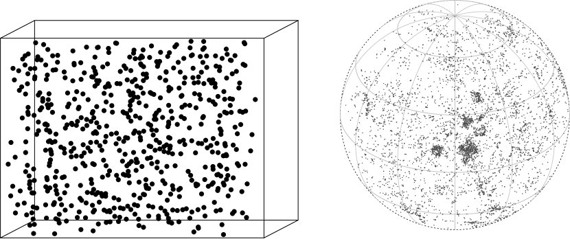
Figure 2: Examples of a point pattern data sets in the $3D$ space and on the sphere. Left: locations of pyramidal brain cells. Right: sky positions of galaxies projected onto the globe. See Section 1.2 for further details.

1.3 Aim and outline

This paper is mainly confined to a review of recent spatial point process models and methods for analyzing spatial point pattern data sets, i.e. without marks or times included and with no ordering on the points. As we have a broad audience in mind, technical details are suppressed. The paper is to some extent a follow-up to our discussion paper Møller & Waagepetersen (2007) which gives a concise and non-technical introduction to the theory of statistical spatial point pattern analysis, making analogies with generalized linear models and random effect models. Thus we mainly focus on developments after the publication of Møller & Waagepetersen (2007) but make no pretense of a complete literature review.

Research in statistical inference for spatial point patterns evolve around the following three main topics:

• development of flexible models for point patterns exhibiting clustering, regularity, trends depending on spatial covariates and combinations of these features;

• methodology for fitting parametric spatial point process models using moment relations or likelihood based methods often implemented using Markov chain Monte Carlo (MCMC) methods;

• development of non-parametric summary statistics for assessing spatial interaction and validating fitted models.

After providing a brief introduction to basic theoretical concepts in Section 2, our exposition follows the above categorization. While much research on modelling has focused on Poisson, Cox, cluster, and Gibbs models (briefly reviewed in Section 3.1), our modelling Section 3 focuses on the classes of determinantal and permanental point processes. The potential of these models for statistical applications has only recently been explored. In addition models characterized by incorporating both clustering and regularity and involving latent geometric structures are reviewed. Section 4 primarily considers estimating function inference where estimating functions are obtained from so-called innovation measures. Maximum likelihood inference for determinantal point processes and Bayesian inference for spatial point processes are reviewed too. Section 5 is concerned with functional summary statistics for non-stationary point processes and new developments in simulation-based inference based on such summary statistics. Finally, Section 6 discusses further recent developments and perspectives for future research.

2 Setting and fundamental concepts

This section specifies our set-up for spatial point processes. For extensions to multiple and marked point processes, and for mathematical details, in particular measure theoretical details, the reader may e.g. consult Møller & Waagepetersen (2004). For instance, below $S$ and $B$ are always Borel sets and $h$ is a measurable function, but we do not emphasize such matters.

Let $S\subseteq\mathbb{R}^{k}$ be the state space for some events, where typically $k=2$ or $k=3$ and often but not always $S$ is of the same dimension, cf. Section 1.1. By a spatial point process on $S$ we mean a locally finite random subset ${\bf X}\subset S$. Letting ${\bf X}_{B}={\bf X}\cap B$ for $B\subseteq S$, locally finite means that the count $N(B)=\#{\bf X}_{B}$ is finite for any bounded $B\subseteq S$. Then the distribution of ${\bf X}$ can be defined by two equivalent approaches: By the finite dimensional distributions of the counts; or, for any bounded $B\subseteq S$, by specifying first the distribution of $N(B)$ and second the distribution of the events in ${\bf X}_{B}$ conditional on knowing $N(B)$. When $S=\mathbb{R}^{k}$ and the distribution of ${\bf X}$ is invariant under translations in $\mathbb{R}^{k}$ respectively rotations about the origin in $\mathbb{R}^{k}$, we say that ${\bf X}$ is stationary respectively isotropic. Similarly, when $d=k-1$, $S=\mathbb{S}^{d}$ is the $d$-dimensional sphere, and the distribution of ${\bf X}$ is invariant under rotations about the origin in $\mathbb{R}^{k}$, we say that ${\bf X}$ is isotropic.

For $n=1,2,\ldots$ and pairwise disjoint bounded sets $B_{1},\ldots,B_{n}\subseteq S$, we define the $n$th order factorial moment measure $\mu^{(n)}(B)$ of the product set $B=B_{1}\times\ldots\times B_{n}$ by the expected value of $\prod_{i=1}^{n}N(B_{i})$. This extends by standard methods to a measure $\mu^{(n)}$ on $S^{n}$ by setting

$$\int_{S^{n}}h(u_{1},\ldots,u_{n})\,\mathrm{d}\mu^{(n)}(u_{1},\ldots,u_{n})=\mathrm{E}\sum^{\not=}_{u_{1},\ldots,u_{n}\in{\bf X}}h(u_{1},\ldots,u_{n})$$

for non-negative functions $h$ defined on $S^{n}$. Here $\not=$ over the summation sign means that $u_{1},\ldots,u_{n}$ are pairwise distinct.

For simplicity and specificity, unless otherwise stated, we assume that $S$ is $k$-dimensional and $\mu^{(n)}$ has a density $\rho^{(n)}$ with respect to Lebesgue measure on $(\mathbb{R}^{k})^{n}$ restricted to $S^{n}$, so that

$$\mathrm{E}\sum^{\not=}_{u_{1},\ldots,u_{n}\in{\bf X}}h(u_{1},\ldots,u_{n})=\int_{S^{n}}h(u_{1},\ldots,u_{n})\rho^{(n)}(u_{1},\ldots,u_{n})\,\mathrm{d}u_{1}\cdots\mathrm{d}u_{n}\,.$$

Then $\rho^{(n)}$ is called the $n$th order joint intensity function. Note that this function is uniquely defined except for a Lebesgue nullset. For pairwise distinct $u_{1},\ldots,u_{n}\in S$, we may interpret $\rho^{(n)}(u_{1},\ldots,u_{n})\,\mathrm{d}u_{1}\cdots\mathrm{d}u_{n}$ as the probability of observing a point in each of $n$ infinitesimally small volumes $\mathrm{d}u_{1},\ldots,\mathrm{d}u_{n}$ containing $u_{1},\ldots,u_{n}$, respectively. If instead e.g. $S=\mathbb{S}^{d}$, then everywhere above we should replace Lebesgue measure with $d$-dimensional surface measure on $\mathbb{S}^{d}$.

The cases $n=1,2$ are of particular interest: $\mu=\mu^{(1)}$ is the intensity measure, $\rho=\rho^{(1)}$ is the intensity function, and the pair correlation function (pcf) is defined for $u,v\in S$ and $u\not=v$ by

$$g(u,v)=\rho^{(2)}(u,v)/\{\rho(u)\rho(v)\}$$

if $\rho(u)\rho(v)>0$, and $g(u,v)=0$ otherwise. The pcf is thus a normalized version of $\rho^{(2)}$ and it is usually easier to interpret: Roughly speaking, the case $g(u,v)=1$ corresponds to that ‘$u$ and $v$ appear independently of each other’, the case $g(u,v)>1$ to that there is ‘attraction between $u$ and $v$’ or ‘aggregation e.g. due to covariates’, and the case $g(u,v)<1$ to that there is ‘inhibition between $u$ and $v$’ or ‘regularity due to the model in question’ (as exemplified later in (h) in Section 3.2.1). Note that this interpretation of $g(u,v)$ may only be meaningful when $u$ and $v$ are sufficiently close. Since the diagonal in $S^{2}$ has zero Lebesgue measure, the definition of $g(u,u)$ can be arbitrary. Depending on the particular model there is often a natural choice as explained later.

If for each $u\in S$, $\pi(u)\in[0,1]$ is a given number, then an independent $\pi$-thinned process ${\bf X}_{{\mathrm{th}}}$ is obtained by independently retaining each point $u\in{\bf X}$ with probability $\pi(u)$. It follows that ${\bf X}_{{\mathrm{th}}}$ has $n$th order joint intensity function $\rho_{{\mathrm{th}}}^{(n)}(u_{1},\ldots,u_{n})=\pi(u_{1})\cdots\pi(u_{n})\rho^{(n)}(u_{1},\ldots,u_{n})$, and the pcf is the same for the two processes.

When $S=\mathbb{R}^{k}$, second order intensity-reweighted stationarity means that $g(u,v)=g_{0}(u-v)$ is invariant under translations in $\mathbb{R}^{k}$. For example, stationarity of ${\bf X}$ implies second order intensity-reweighted stationarity of both ${\bf X}$ and ${\bf X}_{{\mathrm{th}}}$. Baddeley et al. (2000) discuss several other examples of second order intensity-reweighted stationary point processes. If instead $S=\mathbb{S}^{d}$, then second order intensity-reweighted isotropy means that $g(u,v)=g_{0}(d(u,v))$ is invariant under rotations, where $d(u,v)$ is the great circle distance.

We sometimes refer to so-called Palm distributions. The reduced Palm distribution of ${\bf X}$ given a location $u\in S$ can be regarded as the conditional distribution of ${\bf X}\setminus\{u\}$ given that ${\bf X}$ has a point at $u$. We write ${\bf X}^{!}_{u}$ for a spatial point process distributed according to the reduced Palm distribution of ${\bf X}$ given $u$. In the stationary case, ${\bf X}^{!}_{u}$ is distributed as ${\bf X}^{!}_{o}$ translated by $u$, where $o$ denotes the origin, and so we refer to $\mathrm{E}h({\bf X}^{!}_{o})$ as the conditional expectation of $h$ with respect to the further points in ${\bf X}$ given a typical point of ${\bf X}$. Coeurjolly et al. (2015b) give an introduction to Palm distributions intended for a statistical audience.

A useful approach to understanding many models and methods is to consider a subdivision of $S=\cup_{i=1}^{m}C_{i}$ into $m\geq 1$ small cells $C_{i}$ and approximate the spatial point process by a random field of presence-absence binary variables $X_{i}=1[{\bf X}\cap C_{i}\neq\emptyset]$ where $1[A]$ denotes indicator function of an event $A$. That is, $X_{i}=1$ if at least one point is present in the cell $C_{i}$ and $X_{i}=0$ otherwise. By the previously mentioned interpretation, the joint intensities determine the distribution of the binary variables $X_{i}$ associated with a subdivision of $S$ into infinitesimally small cells $C_{i}$. It is also possible to reverse the binary random field point of view. A Poisson process (Section 3.1) for example, can be viewed as a limit of binary random fields of independent binary random variables associated with a sequence of subdivisions for which the cell sizes tend to zero.

3 Models

In Section 3.1 we give a very brief review of Poisson, cluster, Cox, and Gibbs point process models which are covered extensively in the existing literature on spatial point processes, cf. Section 1.1. This is followed by more detailed reviews of recent contributions to the modelling of spatial point processes.

3.1 Poisson, Cox, cluster, and Gibbs point process models

Assume that $\rho$ is an integrable non-negative function on $S$ so that $\mu(B)=\int_{B}\rho(u)\mathrm{d}u$ is finite for all bounded $B\subseteq S$. Then ${\bf X}$ is a Poisson process with intensity function $\rho$ provided that $N(B)$ is Poisson distributed with mean $\mu(B)$ for any bounded $B\subseteq S$ and conditionally on $N(B)=n$, the $n$ points in ${\bf X}_{B}$ are iid on $B$ with density function proportional to $\rho$. The Poisson process has further independence properties:

• For any disjoint subsets $B_{1},\ldots,B_{k}$, $k>1$, of $S$, ${\bf X}_{B_{1}},\ldots,{\bf X}_{B_{k}}$ are independent.

• A Poisson process can be viewed as a limit of binary random fields $\{X_{i}\}_{i=1}^{m}$ associated with increasingly fine subdivisions of $S$ into cells $C_{i}$ of volumes $|C_{i}|$, where the $X_{i}$ are independent with $P(X_{i}=1)=\rho(u_{i})|C_{i}|$ for a representative point $u_{i}\in C_{i}$.

• For any $n\geq 1$, $\rho^{(n)}(u_{1},\ldots,u_{n})=\prod_{i=1}^{n}\rho(u_{i})$.

By the latter property, $g(u,v)=1$ for any pairwise distinct $u,v\in S$ with $\rho(u)\rho(v)>0$, which motivates defining $g(u,u)=1$ on the diagonal of $S^{2}$ for a Poisson process.

Most spatial point pattern data exhibit clustering or regularity that does not comply with the independence properties of a Poisson process. The Poisson process is nevertheless important as a reference process for no spatial interaction. Even more importantly, the Poisson process is the basis for obtaining more flexible models either by specification of probability densities with respect to the Poisson process (Section 3.1.1) or by explicit constructions using Poisson processes as building blocks (Section 3.1.2).

3.1.1 Gibbs point process models

The term Gibbs point processes is in practice used as a broad term for finite point processes specified by a density and their extensions to infinite spatial point processes obtained by considering limits for so-called local specifications, see Møller & Waagepetersen (2004) and the references therein. For simplicity we just consider the finite case below and review various concepts needed later.

Denote by ${\bf Z}$ a finite Poisson process on $S$ with intensity function $\rho$, i.e. $\mu(S)<\infty$. The process ${\bf Z}$ is used as a reference process. If $S$ is bounded, ${\bf Z}$ is often taken to be the unit rate Poisson process with $\rho(\cdot)=1$. Denote by ${\cal N}$ the set of locally finite point configurations of $S$. Suppose that $f$ is a non-negative function on ${\cal N}$ satisfying $\mathrm{E}f({\bf Z})=1$. A spatial point process ${\bf X}$ then has density $f$ on ${\cal N}$ (is absolute continuous) with respect to (the distribution of) ${\bf Z}$ provided

$$\mathrm{E}h({\bf X})=\mathrm{E}\left[h({\bf Z})f({\bf Z})\right]$$

for non-negative functions $h$ on ${\cal N}$. Here, by the definition of a Poisson process,

$$\mathrm{E}h({\bf Z})=\,\sum_{n=0}^{\infty}\frac{\exp[-\mu(S)]}{n!}\,\int_{S}\cdots\int_{S}h({x_{1},\ldots,x_{n}})\rho(x_{1})\cdots\rho(x_{n})\,\mathrm{d}x_{1}\,\cdots\,\mathrm{d}x_{n}.$$ (1)

In the following we consider several examples of point process densities.

If ${\bf X}$ is a finite Poisson process with intensity function $\alpha$ satisfying $\rho(u)>0$ whenever $\alpha(u)>0$, then ${\bf X}$ has density

$$f({\bf x})=\exp\left[\mu(S)-\int_{S}\alpha(u)\mathrm{d}u\right]\prod_{u\in{\bf x}}\frac{\alpha(u)}{\rho(u)},\quad{\bf x}\in{\cal N},$$ (2)

with respect to ${\bf Z}$. If the integral involving $\alpha$ in (2) can not be evaluated analytically, it is at least typically easy to approximate it by numerical integration rendering maximum likelihood inference feasible for parametric models of Poisson processes.

To obtain models with interaction between points, densities are specified in terms of an interaction function $\phi(\cdot)\geq 0$,

$$f({\bf x})=\prod_{{\bf y}\subseteq{\bf x}}\phi({\bf y}).$$

Note that $f({\bf x})$ is proportional to $h({\bf x})=\prod_{{\bf y}\subseteq{\bf x}:{\bf y}\neq\emptyset}\phi({\bf y})$, so $\mathrm{E}f({\bf Z})=1$ is equivalent to

$$\phi(\emptyset)=\frac{1}{\mathrm{E}h({\bf Z})}=\left(\mathrm{E}\prod_{\begin{subarray}{c}{\bf y}\subseteq{\bf Z}:\\ {\bf y}\neq\emptyset\end{subarray}}\phi({\bf y})\right)^{-1}.$$

Thus, $\phi()$ is the normalizing constant that upon multiplication turns $h$ into a probability density. When specifying an interaction function it is important to check that the expectation above defining the normalizing constant is in fact finite. The expectation is typically not available in closed form and must be approximated e.g. by computationally intensive MCMC methods. Often pairwise-only interaction processes are considered in which case $\phi({\bf y})=1$ whenever the cardinality of ${\bf y}$ is greater than two. The Strauss process is the well-known example where for distinct $u,v$, $\phi(\{u\})=\phi(\{v\})=\beta>0$ and $\phi(\{u,v\})=\gamma^{1[\|u-v\|\leq R]}$ for $0<\gamma\leq 1$ and $R>0$. Simulated realizations of the Strauss process for various parameter settings can be found in Møller (1999).

The joint intensities of a spatial point process with density $f$ with respect to ${\bf Z}$ can be expressed as

$$\rho^{(n)}(u_{1},\ldots,u_{n})=\mathrm{E}f(\{u_{1},\ldots,u_{n}\}\cup{\bf Z})$$

for pairwise distinct $u_{1},\ldots,u_{n}$. The expectation on the right hand side is in general not analytically tractable. Fast numerical approximations of the first two joint intensities are developed in Baddeley & Nair (2012a, b).

Suppose $f$ is hereditary meaning that $f({\bf x})>0$ implies $f({\bf y})>0$ for ${\bf y}\subseteq{\bf x}$. Then the $n$-point conditional intensity is defined by

$$\lambda(u_{1},\ldots,u_{n},{\bf x})=\frac{f(\{u_{1},\ldots,u_{n}\}\cup{\bf x})}{f({\bf x})}$$

for pairwise distinct $u_{1},\ldots,u_{n}$ and finite point configurations ${\bf x}$ with ${\bf x}\cap\{u_{1},\ldots,u_{n}\}=\emptyset$. The conditional intensities e.g. play an important role in the definition of innovation measures for Gibbs point processes, see Section 4.1.

3.1.2 Cox and cluster processes

A large class of models for random spatial aggregation of points is obtained by replacing the deterministic intensity function in a Poisson process by a random function. More precisely, let $\mathbf{\Lambda}=\{\Lambda(u)\}_{u\in S}$ be a non-negative random field such that $\mathbf{\Lambda}$ is locally integrable almost surely (that is, for bounded $B\subseteq S$, $\int_{B}\Lambda(u)\,\mathrm{d}u$ exists and is finite with probability one). Then ${\bf X}$ is a Cox process provided that conditional on ${\mathbf{\Lambda}}={\mathbf{\lambda}}$, ${\bf X}$ is a Poisson process with intensity function ${\mathbf{\lambda}}$. The joint intensities are simply given by

$$\rho^{(n)}(u_{1},\ldots,u_{n})={\mathbb{E}}\prod_{i=1}^{n}\Lambda(u_{i})$$

for $n\geq 1$ and pairwise distinct $u_{1},\ldots,u_{n}\in S$. For a log Gaussian Cox process, i.e. when $\log\Lambda$ is a Gaussian process, $\rho^{(n)}$ is just given by the Laplace transform of a multivariate normal distribution (Møller et al., 1998).

To obtain clustered point patterns, one way is to consider superpositions of a countable number of localized point processes. Accordingly, a Poisson cluster process is a union ${\bf X}=\cup_{v\in{\mathbf{\Phi}}}{\bf X}_{v}$ of typically finite spatial point processes ${\bf X}_{v}$ on $S$ indexed by a parent Poisson process ${\mathbf{\Phi}}$ on $S$ or perhaps some other space. For convenience, conditional on ${\mathbf{\Phi}}$, the ${\bf X}_{v}$ are often assumed to be finite Poisson processes each with intensity function $\rho_{v}$, in which case ${\bf X}$ can also be viewed as a Cox process with random intensity function ${\mathbf{\Lambda}}(u)=\sum_{v\in{\mathbf{\Phi}}}\rho_{v}(u)$. Shot-noise Cox processes is a specific example of this, where ${\mathbf{\Phi}}$ is a Poisson process on $\mathbb{R}^{d}\times]0,\infty[$ and for a $v=(c,\gamma)\in{\mathbf{\Phi}}$, $\rho_{v}(u)=\gamma k(c,u)$, where $k(c,\cdot)$ is a probability density on $S$ (Møller, 2003). Simulated realizations of log Gaussian and Poisson cluster processes can be found in Chapter 5 in Møller & Waagepetersen (2004).

At the expense of analytical tractability, Poisson parent processes can be replaced e.g. by regular parent processes (Van Lieshout & Baddeley, 2002; McKeague & Loizeaux, 2002; Møller & Torrisi, 2005) and the Poisson distribution for cluster size could be replaced by other integer valued distributions. Jalilian et al. (2013) introduce a flexible class of shot-noise Cox processes with kernel function $k$ given by the density of normal-variance mixture distributions. For this class of models, the pair correlation function is given by $g(u,v)=1+c(u,v)$ where $c(u,v)$ is a covariance function given by a scaled normal-variance mixture density. This includes e.g. Matérn and Cauchy covariance functions. Most examples of Cox process models are second order intensity-reweighted stationary, with an isotropic pcf. Møller & Toftager (2014) study Cox process models with an elliptical pcf, including shot noise Cox processes and log Gaussian Cox processes.

The density of a finite Cox process with respect to a finite Poisson process ${\bf Z}$ is

$$f({\bf x})=\mathrm{E}f({\bf x}|\Lambda)$$

where $f(\cdot|{\mathbf{\lambda}})$ is the conditional density of ${\bf X}$ given ${\mathbf{\Lambda}}={\mathbf{\lambda}}$ with respect to ${\bf Z}$. The expectation can rarely be computed analytically. Likelihood based inference for Cox processes therefore typically require numerical (including Monte Carlo) approximations of the likelihood function.

3.2 Determinantal and permanental point processes

Macchi (1975) introduced two interesting models motivated by fermions and bosons in quantum mechanics, viz. determinantal and permanental point processes.

3.2.1 Determinantal point processes

Determinantal point processes (DPPs) are of interest because of their applications in mathematical physics, combinatorics, random-matrix theory, machine learning, and spatial statistics (see Lavancier et al., 2015, and the references therein). For DPPs on $\mathbb{R}^{k}$, rather flexible parametric models can be constructed and likelihood and moment based inference procedures apply (Lavancier et al., 2014, 2015). DPPs on the sphere are discussed from a statistical perspective in Møller et al. (2015a) and Møller & Rubak (2016).

A DPP is defined by a function $C:S\times S\mapsto\mathbb{C}$ as follows: ${\bf X}$ is a DPP with kernel $C$ if for any $n=1,2,\ldots$, ${\bf X}$ has a non-negative $n$th order joint intensity function given by

$$\rho^{(n)}(u_{1},\ldots,u_{n})=\det\left(C(u_{i},u_{j})_{i,j=1,\ldots,n}\right)\quad\mbox{for all $u_{1},\ldots,u_{n}\in S$},$$ (3)

where $\det\left(C(u_{i},u_{j})_{i,j=1,\ldots,n}\right)$ is the determinant of the $n\times n$ matrix with $(i,j)$th entry $C(u_{i},u_{j})$. Then we write ${\bf X}\sim\text{DPP}(C)$.

Before discussing the existence of this process, several points are in order when we assume ${\bf X}\sim\text{DPP}(C)$ exists (in fact it is then unique).

1. The kernel can be complex, since this becomes convenient when considering simulation of DPPs as discussed below. In statistical models, it is usually real.

2. A Poisson process on $S$ with intensity function $\rho$ is the special case of a DPP where $C(u,u)=1$ and $C(u,v)=0$ for $u\not=v$.

3. The intensity function is $\rho(u)=C(u,u)$, and the pcf is $g(u,v)=1-|C(u,v)|^{2}/\{C(u,u)C(v,v)\}$. Thus $g(u,u)=0$.

4. By (3), an independent $\pi$-thinning of ${\bf X}\sim\text{DPP}(C)$ results in ${\bf X}_{{\mathrm{th}}}\sim\text{DPP}(C_{{\mathrm{th}}})$, where $C_{{\mathrm{th}}}(u,v)=\sqrt{\pi(u)\pi(v)}C(u,v)$. Thus, if $C(u,v)=C_{0}(u-v)$ is stationary, ${\bf X}_{{\mathrm{th}}}$ is second order intensity-reweighted stationary (on the sphere this holds provided $C(u,v)=C_{0}(d(u,v))$ is isotropic).

5. In particular, for any $B\subseteq S$, ${\bf X}_{B}$ is a DPP on $B$, with the restriction of $C$ to $B\times B$ as its kernel. This is in contrast to Gibbs point processes. For example, the restriction of a Strauss process to a smaller region is not a Strauss process and its density is intractable even up to a constant of proportionality.

6. A smooth one-to-one transformation of ${\bf X}$ results in a new DPP, cf. Lavancier et al. (2014).

7. By (3) and since $\rho^{(n)}$ is non-negative, $C$ has to be positive semi-definite. In fact, in most work on DPPs, the kernel is assumed to be Hermitian, i.e. $C$ is a complex covariance function. In the sequel, we make this assumption.

8. By (c) this implies that $g\leq 1$, which usually is a strict inequality, i.e. there is ‘regularity at any scale’. In fact, an even stronger result holds: for all $u_{1},\ldots,u_{n}\in S$ we have $\rho^{(n)}(u_{1},\ldots,u_{n})\leq\rho(u_{1})\cdots\rho(u_{n})$, with equality if and only if ${\bf X}$ is a Poisson process with intensity function $\rho$.

The existence of ${\bf X}\sim\text{DPP}(C)$ relies on a spectral representation of the kernel: Consider $C$ restricted to any compact set $B\subseteq S$. Under mild conditions (e.g. continuity of $C$ is sufficient, cf. Lavancier et al., 2014, 2015), for any $u,v\in B$,

$$C(u,v)=\sum_{i=1}^{\infty}\lambda_{i}\phi_{i}(u){\overline{\phi_{i}(v)}},$$ (4)

where $\overline{z}$ denotes complex conjugate of $z\in\mathbb{C}$, $\lambda_{i}$ is the eigenvalue corresponding to the eigenfunction $\phi_{i}$, and $\int_{B}\phi_{i}(u){\overline{\phi_{j}(u)}}\,\mathrm{d}u=1[i=j]$. Then existence is equivalent to that all $\lambda_{i}\leq 1$, cf. Lavancier et al. (2014, 2015) and the references therein. If $S=\mathbb{R}^{k}$ and $C(u,v)=C_{0}(u-v)$ is stationary, under mild conditions existence is equivalent to that the spectral density for $C_{0}$ is at most 1 (Lavancier et al., 2014, 2015). If $S=\mathbb{S}^{d}$ and ${\bf X}$ is isotropic, the eigenfunctions are given by spherical harmonics, see Møller et al. (2015a).

Lavancier et al. (2014, 2015) conclude that DPPs offer relatively flexible models for repulsiveness, although less flexible than Gibbs point processes, e.g. DPPs cannot be as repulsive as Gibbs hard-core point processes can be. This is due to the bound on the spectrum of $C$ needed for the existence of ${\bf X}\sim\text{DPP}(C)$: The bound implies a trade-off between a large intensity and a strong degree of interaction.

The spectral decomposition allows a closed form expression for the likelihood when ${\bf X}$ is observed within a compact region, but in practice the likelihood needs to be approximated as discussed later in Section 4.4. Furthermore, $N(B)$ is distributed as $\sum_{i=1}^{\infty}N_{i}$, where $N_{1},N_{2},\ldots$ are independent Bernoulli variables with parameters $\lambda_{1},\lambda_{2},\ldots$. Simulation of $N_{1},N_{2},\ldots$ is easy and conditional on $N_{1},N_{2},\ldots$, the events in ${\bf X}_{B}$ can be generated one by one using a fast exact simulation procedure based on the fact that ${\bf X}_{B}$ has a density which is proportional to the $(\sum_{i=1}^{\infty}N_{i})$th order intensity function for a DPP with kernel $\sum_{i=1}^{\infty}N_{i}\phi_{i}(u){\overline{\phi_{i}(v)}}$. See Hough et al. (2006) and Lavancier et al. (2014, 2015).

To summarize, in comparison to Gibbs point processes, DPPs possess many appealing properties: DPPs can be easily simulated; their moments and the likelihood are tractable; a DPP restricted to a smaller region is again a DPP; an independent thinning of a DPP or a smooth one-to-one transformation is again a DPP; and the distribution of the number of events within a compact region is known.

3.2.2 Permanental point processes and extensions

Given a complex covariance function $C:S\times S\mapsto\mathbb{C}$, ${\bf X}$ is a permanental point process (PPP) with kernel $C$ if for any $n=1,2,\ldots$, ${\bf X}$ has a non-negative $n$th order intensity function as in (3) but with the determinant replaced by the permanent

$$\mathrm{per}\left(C(u_{i},u_{j})_{i,j=1,\ldots,n}\right)=\sum_{(\sigma_{1},\ldots,\sigma_{n})}\prod_{i=1}^{n}C(u_{\sigma_{i}},u_{\sigma_{j}}),$$

where the sum is over all permutations of $1,\ldots,n$. In fact, ${\bf X}$ is then a Cox process driven by $|{\bf Z}|^{2}$, where ${\bf Z}$ is a zero-mean complex Gaussian process with covariance function $C$. The intensity function is $\rho(u)=C(u,u)$ and the pcf is $g(u,v)=1+|C(u,v)|^{2}/\{C(u,u)C(v,v)\}$. This implies that $g\geq 1$ which usually is a strict inequality, i.e. there is ‘aggregation at any scale’.

Despite some attractive properties of PPPs (Hough et al., 2006; McCullagh & Møller, 2006), including that the spectral decomposition (4) allows a closed form expression for the likelihood when ${\bf X}$ is restricted to a compact set, PPPs have yet not been used much in applications, probably because computing permanents is computationally infeasible even for relatively small matrices. Since $1\leq g\leq 2$, PPPs may be a rather restrictive class of models for aggregation. Nevertheless, we think PPPs deserve to be investigated more because of their attractive moment properties.

Determinantal and permanental point processes can be extended by replacing the determinant or permanent with a weighted determinant or permanent, see McCullagh & Møller (2006). This extension includes the case of a Cox process driven by $\sum_{i=1}^{k}{\bf Y}_{i}^{2}$, where ${\bf Y}_{1},{\bf Y}_{2},\ldots$ are independent zero-mean real Gaussian processes with a common real covariance function $C$.

3.3 Regularity on the small scale and aggregation on the large scale

In the classical spatial point process literature, spatial point processes are often classified into three main cases, viz. complete spatial randomness (i.e. the Poisson process), regularity (e.g. DPPs and most Gibbs point processes), and aggregation (e.g. Cox processes). This can be too simplistic, and often we need a model with aggregation on the large scale and regularity on the small scale.

Gibbs point processes with an inhomogeneous first order potential and inhibitive pairwise interactions are models for deterministic aggregation combined with inhibition at the small scale. Alternatively, in order to introduce inhomogeneity, homogeneous regular Gibbs processes can be subjected to location dependent thinning, smooth transformation, or local scaling (Baddeley et al., 2000; Jensen & Nielsen, 2000; Hahn et al., 2003). Another possibility is to consider a homogeneous Gibbs point process with a well-chosen higher-order potential that incorporates inhibition at small scales and attraction at large scales. A famous example is the Lennard-Jones pair-potential (Ruelle, 1969). Another specific potential of this type can be found in Goldstein et al. (2015). Disadvantages of Gibbs point process models or models derived from those are that densities and joint intensities are intractable and that simulation requires elaborate MCMC methods, cf. Section 3.1.1.

In the following we focus on two modeling strategies to obtain random aggregation as well as random local regularity. In Andersen & Hahn (2015) the starting point is a (aggregated) Cox process which is subjected to dependent thinning to create local regularity. Conversely, Lavancier & Møller (2016) begin with a (regular) determinantal point process and use randomly spatially varying thinning to obtain aggregation.

Specifically, Andersen & Hahn (2015) apply Matérn type II dependent thinning to shot-noise Cox processes (Section 3.1.2). For a given point pattern and a specified distance $h$, Matérn II thinning acts by first attaching random positive marks (‘arrival times’) to each point. Subsequently a point is removed if it has a neighbour within distance $h$ and with a smaller mark (i.e. the neighbour arrived earlier). For a given location $u$, Andersen & Hahn (2015) define the retention probability at $u$ as the ratio between the intensities of the thinned process and the orginal process at $u$. They derive expressions for the retention probabilities in terms of integrals that, however, must be evaluated using numerical integration. Simple approximate formulae for the intensity function and the second-order joint intensity of the thinned process are also provided and used for fitting of parametric models to data sets of cell centres in microscopial images of bone marrow tissue.

On the other hand, Lavancier & Møller (2016) consider a spatial point process ${\bf Y}$ on $S$ and a random field $\Pi=\{\Pi(x):x\in S\}$ of retention probabilities independent of ${\bf Y}$. Conditional on $\Pi$, ${\bf X}$ is then an independent thinning of ${\bf Y}$ with retention probabilities $0\leq\Pi(u)\leq 1$ at $u\in S$. In Stoyan (1979) and Chiu et al. (2013), ${\bf X}$ is called an interrupted point process (which is a good terminology when each $\Pi(x)$ is either 0 or 1). Simple relations between the intensity and pair correlation functions of ${\bf Y}$ and ${\bf X}$ are then available:

$$\rho_{{\bf X}}(u)=q(u)\rho_{{\bf Y}}(u),\quad q(u)=\mathrm{E}\Pi(u),\quad u\in S,$$ (5)

and (setting $0/0=0$)

$$g_{{\bf X}}(u,v)=M(u,v)g_{{\bf Y}}(u,v),\quad M(u,v)=\frac{\mathrm{E}[\Pi(u)\Pi(v)]}{\mathrm{E}[\Pi(u)]\mathrm{E}[\Pi(v)]},\quad u,v\in S.$$ (6)

For example, if $g_{{\bf Y}}\leq 1$ while $\Pi$ is positively correlated (i.e. $M>1$), then we may achieve $g_{{\bf X}}$ smaller/larger than 1 on the small/large scale. In the cases where ${\bf Y}$ is a determinantal point process or a Matérn hard core model of type I or II (Matérn, 1986) and $\Pi$ is based on a transformed Gaussian process or the characteristic function of a Boolean model of balls, Lavancier & Møller (2016) derive explicit formulae for $\rho_{\bf X}$ and $g_{{\bf X}}$. For such models, simulation of $({\bf Y},\Pi,{\bf X})$ restricted to a bounded region is furthermore straightforward. Conditional simulation of $\Pi$ given ${\bf X}$, ${\bf Y}$ or both is more complicated and discussed in Lavancier & Møller (2016).

3.4 Latent geometric structures

Spatial point processes in the neighbourhood of a reference structure are frequently observed. Often the reference structure has a kind of linear structure. A diverse set of examples at very different scales are gold coins near Roman roads (pp. 226–229 in Hodder & Orton, 2013), copper deposits in the neighbourhood of lineaments (Berman, 1986; Baddeley & Turner, 2006; Illian et al., 2008), galaxies at the boundary of cosmic voids (Icke & Van de Weygaert, 1987; Van de Weygaert & Icke, 1989; Van de Weygaert, 1994), pores at the boundary of grains (Karlsson & Liljeborg, 1994; Skare et al., 2007), animal latrines near territorial boundaries (Blackwell, 2001; Blackwell & Møller, 2003; Skare et al., 2007), linear rows of mines (Walsch & Raftery, 2002), specific tree species along rivers in a rain forest (Valencia et al., 2004), and brain cells with a columnar structure (cf. Figure 2). In many cases the reference structure is not easy to recognize. The objective of the statistical analysis of point patterns of this type may either be to describe the distribution of the point pattern or to reconstruct the reference structure or perhaps both.

For example, as in Blackwell (2001), Blackwell & Møller (2003), and Skare et al. (2007), the unknown reference structure may be modelled by a Voronoi tessellation and the points of an unknown point process on the edges of this tessellation are randomly disturbed to produce an observed point pattern with points around the edges. Such complex models are analyzed in a Bayesian MCMC setting with priors on the spatial point process of nuclei generating the Voronoi tessellation, the point process on the edges, and the model parameters. Typically, for tractability, the spatial point process priors are Poisson processes, in which case the likelihood for the observed point pattern is described by a Cox process where the driving intensity is specified by the nuclei and the model parameters. The posterior then just concerns the Voronoi tessellation and the model parameters, and a major element of the MCMC algorithm is the reconstruction of the Voronoi tessellation after a proposed local change of the tessellation.

The construction above is in Møller & Rasmussen (2015) extended to construct models for cluster point processes within territories modelled by the Voronoi cells, where conditional on the territories/cells, the clusters are independent Poisson processes whose points may be aggregated around or away from the nuclei and along or away from the boundaries of the cells.

To model a columnar structure for the pyramidal cell data set in Figure 2, a hierarchical construction starting with a Poisson line process $\mathbf{L}$ is used in Møller et al. (2015b): Consider on each line $l_{i}$ of $\mathbf{L}$ a Poisson process ${\bf Y}_{i}$ and let ${\bf X}_{i}$ be obtained by random displacements of the points in ${\bf Y}_{i}$. Then ${\bf X}$ is the superposition of all the ${\bf X}_{i}$. For this model Møller et al. (2015b) discuss moment results and simulation procedures based on the fact that ${\bf X}$ becomes a Cox process which is closely related to a shot-noise Cox process where the centre process is replaced by $\mathbf{L}$. Simulation of ${\bf X}$ within a bounded observation window needs to take care of edge effects, and conditional simulation of its random intensity (when ${\bf X}$ is viewed as a Cox process) requires MCMC techniques; for details, see Møller et al. (2015b). In the case where all the lines are parallel and their direction is known (this is a reasonable assumption for the pyramidal brain cell data set), the pcf is tractable and useful for inference.

4 Estimation

In this section we assume that ${\bf X}$ is observed within a bounded set $W\subseteq S$ and that a parametric model has been specified for the distribution of ${\bf X}$ or alternatively just for the joint intensities $\rho^{(n)}$ for some $n\geq 1$ (often just the intensity and pair correlation functions are considered, i.e. $n=1,2$). The unknown parameter to be estimated is denoted $\theta$ and assumed to be real of dimension $p$, and we write $\rho^{(n)}(\cdot;\theta)$, $\lambda^{(n)}(\cdot;\theta)$ etc. to stress the dependence on $\theta$.

In the case of a Gibbs process where the likelihood is specified, maximum likelihood inference and Bayesian inference is in general difficult due to the complicated normalizing constant. The Poisson process is one exception where the modest computational challenge is the evaluation of an integral over the observation window $W,$ cf. (2). For Cox and cluster processes, the likelihood function is also very complicated, involving expectations with respect to the unobserved random intensity function or the unobserved parent points. Approximate maximum likelihood or Bayesian inference may be implemented using Monte Carlo methods or Laplace approximations (see e.g. Møller & Waagepetersen, 2004, 2007, for reviews). Some comments on maximum likelihood inference for determinantal point processes are given in Section 4.4 while Section 4.5 discusses some points regarding Bayesian inference.

Due to the computational obstacles related to likelihood based inference, much interest has focused on establishing computationally easier approaches for spatial point processes with specified conditional intensity in the case of Gibbs processes and specified intensity and pair correlation functions in the case of Cox and cluster processes. This includes Takacs-Fiksel and pseudolikelihood estimation for Gibbs point processes (e.g. Besag, 1977; Fiksel, 1984; Takacs, 1986; Jensen & Møller, 1991; Diggle et al., 1994; Billiot, 1997; Baddeley & Turner, 2000; Billiot et al., 2008; Coeurjolly et al., 2012) and various types of minimum contrast, composite likelihood, Palm likelihood and estimating functions for Cox and cluster processes and DPPs (e.g. Schoenberg, 2005; Guan, 2006; Waagepetersen, 2007; Tanaka et al., 2008; Waagepetersen & Guan, 2009; Dvořák & Prokešová, 2012; Prokešová & Jensen, 2013; Prokešová et al., 2014; Guan et al., 2015; Zhuang, 2015; Lavancier et al., 2014, 2015). As discussed in Sections 4.1-4.3, all of these methods belong to a common framework of estimating functions based on signed innovation measures (Baddeley et al., 2005; Waagepetersen, 2005; Zhuang, 2006).

4.1 Innovation measures and estimating functions

For a spatial point process with $n$’th order joint intensity $\rho^{(n)}$, we define the $n$’th order innovation measure as

$$I^{(n)}(B_{1}\times\cdots\times B_{n})$$

$$= \sum_{u_{1},\ldots,u_{n}\in{\bf X}}^{\neq}1[u_{1}\in B_{1},\ldots,u_{n}\in B_{n}]-\int_{B_{1}\times\cdots\times B_{n}}\rho^{(n)}(u_{1},\ldots,u_{n})\,\mathrm{d}u_{1}\cdots\mathrm{d}u_{n}$$

for $B_{i}\subseteq S$, $i=1,\ldots,n$. By definition of the factorial moment measure, $I^{(n)}(B_{1}\times\cdots\times B_{n})$ has expectation zero. For Gibbs point processes the factorial moment measure is not known in closed form and it is more convenient to define conditional innovation measures in terms of the $n$’th order conditional intensity: For $F$ a set of locally finite point configurations and $B_{i}$ as above,

$$I^{(n)}(B_{1}\times\cdots\times B_{n}\times F|{\bf X})$$

$$= \sum_{u_{1},\ldots,u_{n}\in{\bf X}}^{\neq}1[u_{1}\in B_{1},\ldots,u_{n}\in B_{n},{\bf X}\setminus\{u_{1},\ldots,u_{n}\}\in F]$$

$$-\int_{B_{1}\times\cdots\times B_{n}}1[{\bf X}\in F]\lambda^{(n)}(u_{1},\ldots,u_{n},{\bf X})\,\mathrm{d}u_{1}\cdots\mathrm{d}u_{n}$$

which has expectation zero by the Georgii-Nguyen-Zessin formula (Georgii, 1976; Nguyen & Zessin, 1979).

Introducing the dependence on $\theta$ as well as $p$-dimensional weight functions $h(\cdot;\theta)$ on $S^{n}$ or on $S^{n}\times{\mathcal{N}}$, we then obtain classes of $n$’th order unbiased estimating functions

$$e_{h}^{(n)}(\theta)= \int_{W^{n}}h(u_{1},\ldots,u_{n};\theta)I^{(n)}(\mathrm{d}u_{1}\cdots\mathrm{d}u_{n};\theta)$$

$$= \sum_{u_{1},\ldots,u_{n}\in{\bf X}_{W}}^{\neq}h(u_{1},\ldots,u_{n};\theta)-\int_{W^{n}}h(u_{1},\ldots,u_{n};\theta)\rho^{(n)}(u_{1},\ldots,u_{n};\theta)\,\mathrm{d}u_{1}\cdots\mathrm{d}u_{n}$$ (7)

or

$$e_{h}^{\text{tf},(n)}(\theta)= \int_{W^{n}\times{\mathcal{N}}}h(u_{1},\ldots,u_{n},{\bf z};\theta)I^{(n)}(\mathrm{d}u_{1}\cdots\mathrm{d}u_{n}\mathrm{d}{\bf z}|{\bf X};\theta)$$

$$= \sum_{u_{1},\ldots,u_{n}\in{\bf X}_{W}}^{\neq}h(u_{1},\ldots,u_{n},{\bf X}\setminus\{u_{1},\ldots,u_{n}\};\theta)$$

$$-\int_{W^{n}}h(u_{1},\ldots,u_{n},{\bf X};\theta)\lambda^{(n)}(u_{1},\ldots,u_{n},{\bf X};\theta)\,\mathrm{d}u_{1}\cdots\mathrm{d}u_{n}.$$ (8)

Here unbiasedness means that $\mathrm{E}e_{h}^{(n)}(\theta)=\mathrm{E}e_{h}^{\text{tf},(n)}(\theta)=0$, with the expectations calculated under $\theta$. We will use the term Takacs-Fiksel estimating function for an estimating function of the type (8). For Takacs-Fiksel estimating functions we may account for edge effects by letting $W$ be an eroded observation window, see e.g. Møller & Waagepetersen (2004).

4.2 Estimating functions based on joint intensity functions

In practice estimating functions of the form (7) are mainly considered in the first ($n=1$) or second order ($n=2$) cases and can be motivated by composite likelihood arguments.

4.2.1 Composite likelihood

The first notion of composite likelihood for spatial point processes is due to Guan (2006) who defined a bivariate probability density $f(u,v;\theta)\propto\rho^{(2)}(u,v;\theta)$, $u,v\in W,$ and considered the log composite likelihood $\sum_{u,v\in{\bf X}}^{\neq}\log f(u,v;\theta)$. Below we discuss and compare other approaches to composite likelihood for spatial point processes based on the infinitesimal interpretation of joint intensity functions.

Letting $h(u;\theta)=\mathrm{d}\log\rho(u;\theta)/\mathrm{d}\theta$ in (7) in the case $n=1$, the score of the Poisson log likelihood is recovered. If the underlying spatial point process is not Poisson, the estimating function can be interpreted as a composite likelihood score for the binary indicators $X_{i}$ of presence of points in cells of an infinitesimal partition of the observation window mentioned in the end of Section 2 (Schoenberg, 2005; Waagepetersen, 2007; Guan & Loh, 2007; Møller & Waagepetersen, 2007). Likewise, in case $n=2$ with $h(u,v;\theta)=1[\|u-v\|\leq R]\,\mathrm{d}\log\rho^{(2)}(u,v;\theta)/\mathrm{d}\theta$ for some tuning parameter $R>0$, the score of a second order composite likelihood

$$\sum_{u,v\in{\bf X}_{W}}^{\neq}1[\|u-v\|\leq R]\frac{\mathrm{d}}{\mathrm{d}\theta}\log\rho^{(2)}(u,v;\theta)-\int_{W^{2}}1[\|u-v\|\leq R]\frac{\mathrm{d}}{\mathrm{d}\theta}\rho^{(2)}(u,v;\theta)\mathrm{d}u\mathrm{d}v$$ (9)

is obtained — this time for binary indicators $X_{i}X_{j}$ of simultaneous occurrence of points in $R$-close pairs of distinct cells $C_{i}$ and $C_{j}$ of the aforementioned partition (Waagepetersen, 2007; Møller & Waagepetersen, 2007). Returning to Guan (2006)’s composite likelihood the associated score is

$$\sum_{u,v\in{\bf X}_{W}}^{\neq}1[\|u-v\|\leq R]\frac{\mathrm{d}}{\mathrm{d}\theta}\log\rho^{(2)}(u,v;\theta)-\sum_{u,v\in{\bf X}_{W}}^{\neq}\frac{\int_{W^{2}}\frac{\mathrm{d}}{\mathrm{d}\theta}1[\|u-v\|\leq R]\rho^{(2)}(u,v;\theta)\,\mathrm{d}u\mathrm{d}v}{\int_{W^{2}}1[\|u-v\|\leq R]\rho^{(2)}(u,v;\theta)\,\mathrm{d}u\mathrm{d}v}.$$ (10)

The estimating functions (9) and (10) are closely related since their first terms agree. Moreover, the expectation of the last term in (10) coincides with the last term in (9) so that (10) is also unbiased.

The so-called Palm likelihood (Tanaka et al., 2008) is based on composite likelihood arguments too. For a fixed point $u\in\mathbb{R}^{d}$ the reduced Palm spatial point process ${\bf X}_{u}^{!}$ has intensity function $\rho(v|u;\theta)=\rho^{(2)}(u,v;\theta)/\rho(u;\theta)$. Assuming that ${\bf X}$ is stationary with known constant intensity, the unbiased score (Prokešová & Jensen, 2013) of the Palm likelihood is

$$\sum_{u\in{\bf X}_{W}}\sum_{v\in{\bf X}\setminus u}\frac{\mathrm{d}}{\mathrm{d}\theta}\log\rho(v|u;\theta)1[\|v-u\|\leq R]-N\left({\bf X}_{W}\right)\int_{\|v\|\leq R}\frac{\mathrm{d}}{\mathrm{d}\theta}\rho(v|o)\mathrm{d}v.$$ (11)

Obviously, considering the first term in (11), the Palm likelihood is closely related to the two other types of second order composite likelihoods.

Asymptotic results for the various types of composite likelihoods are provided in Guan (2006), Waagepetersen (2007), Guan & Loh (2007), Waagepetersen & Guan (2009), and Prokešová & Jensen (2013). It is not known which type of composite likelihood is most efficient. In any case, none of them are optimal, see Section 4.2.2.

4.2.2 Quasi-likelihood

While the estimating functions described in the previous setting have a nice motivation in terms of composite likelihoods, they are in general not optimal. Optimality can be achieved following the route of quasi-likelihood.

For an $m\times 1$ data vector $Y$ with mean vector $\mu$ depending on a $p$-dimensional parameter $\theta$, a class of unbiased estimating functions are given by

$$A^{\mbox{\scriptsize\sf T}}(Y-\mu)$$

for $m\times p$ matrices $A$. This can be viewed as a matrix-vector analogue of the estimating function (7) in case $n=1$ with $Y-\mu$ and $A$ corresponding to the innovation process $I^{(n)}$ and the weight function $h$, respectively. The optimal choice of $A$ is the solution of $VA=D$ where $D$ is the $m\times p$ matrix of partial derivatives $\mathrm{d}\mu_{i}/\mathrm{d}\theta_{j}$ and $V$ is the covariance matrix of $Y$. This choice of $A$ yields the so-called quasi-likelihood score (e.g. Heyde, 1997).

Guan et al. (2015) generalize the concept of quasi-likelihood to the case of spatial point processes. Considering the class of first order estimating functions (7) they identify the optimal weight function $h$ as the solution of a Fredholm integral equation

$$h+Th=\frac{\mathrm{d}}{\mathrm{d}\theta}\log\rho(\cdot,\theta)$$

where $T$ is a certain integral operator depending on the pair correlation function of the spatial point process. They further establish asymptotic properties of the spatial point process quasi-likelihood and also provide an efficient numerical implementation of the method.

Guan et al. (2016) take the quasi-likelihood idea further and consider a second order quasi-likelihood giving the optimal choices of $h_{1}$ and $h_{2}$ for the linear combination

$$e^{(1)+(2)}_{h_{1},h_{2}}(\theta)=e^{(1)}_{h_{1}}(\theta)+e^{(2)}_{h_{2}}(\theta).$$

This leads to considerable computational challenges as the optimal functions $h_{1}$ and $h_{2}$ now depend also on third and fourth order joint densities. However, in the stationary case, Guan et al. (2016) show that restricting attention to constant functions $h_{1}$ and functions $h_{2}$ with $h_{2}(u,v)$ only depending on $v-u$ does not lead to a loss of efficiency asymptotically and moreover simplifies computations greatly.

Given a set of estimating functions $e_{1}(\theta),\ldots,e_{m}(\theta)$, a related topic is to obtain a combined estimating function as an optimal linear combination $e(\theta)=\sum_{i=1}^{m}A_{i}e_{i}(\theta)$ for $p\times p$ matrices $A_{i}$. The weight matrices $A_{i}$ can be determined according to quasi-likelihood arguments and this approach is considered in Deng et al. (2015) for estimation of parameters in stationary point processes. Similarly, Lavancier & Rochet (2016) consider how to obtain an estimate as an optimal linear combination $\hat{\theta}=\sum_{i=1}w_{i}\hat{\theta}_{i}$ given a collection of estimates $\hat{\theta}_{1},\ldots,\hat{\theta}_{m}$ of the same parameter $\theta$.

4.2.3 Case-control likelihood

Consider (7) with $n=1$ and $h(u)=\mathrm{d}\log\rho(u;\theta)/\mathrm{d}\theta$. Suppose in addition to ${\bf X}$ another spatial point process ${\bf Z}$ of intensity $\alpha$ is available where ${\bf X}$ and ${\bf Z}$ are almost surely disjoint. Then

$$\sum_{u\in{\bf X}\cup{\bf Z}}\frac{\mathrm{d}\rho(u;\theta)/\mathrm{d}\theta}{\rho(u;\theta)+\alpha(u)}$$ (12)

is an unbiased estimate of the last integral in (7). The estimating function obtained by replacing the integral by the unbiased estimate (12) is the derivative of

$$\sum_{u\in{\bf X}}\log\frac{\rho(u;\theta)}{\rho(u;\theta)+\alpha(u)}+\sum_{u\in{\bf Z}}\log\frac{\alpha(u)}{\rho(u;\theta)+\alpha(u)}$$ (13)

which is the limit of log conditional likelihoods based on the conditional distribution of binary indicators $X_{i}$ given $X_{i}+Z_{i}=1$ where the $Z_{i}$ are presence/absence indicators for ${\bf Z}$. Thus, in epidemiological terminology, ${\bf X}$ and ${\bf Z}$ play the role of case and control processes.

Diggle & Rowlingson (1994) introduced (13) in the case where ${\bf Z}$ is a spatial point process representing a background population and ${\bf X}$ is a spatial point process of disease cases with intensity function

$$\rho(u;\theta)=f(u;\theta)\alpha(u).$$

In this setup $\alpha$ is assumed to be unknown but cancels out in both terms of (13). Waagepetersen (2008) considers the case where ${\bf Z}$ is a user generated dummy point process generated with the sole purpose of approximating the integral. Guan et al. (2008) generalize (13) to the case of second order joint intensities. Diggle et al. (2010), Huang et al. (2014), and Chang et al. (2015) further exploit and expand the case control methodology for spatial point processes in epidemiological applications with multiple sources of data.

4.3 Pseudo-likelihood

Estimating functions of the type (8) have so far mainly been considered when $n=1$ in which case the by far most popular weight function is $h(u,{\bf x})=\mathrm{d}\log\lambda(u,{\bf x};\theta)/\mathrm{d}\theta$ leading to the pseudo-likelihood score (e.g. Besag, 1977; Jensen & Møller, 1991; Baddeley & Turner, 2000; Billiot et al., 2008). A review of other choices of weight functions is provided in Coeurjolly et al. (2012) who also introduce weight functions designed to lead to computationally quick Takacs-Fiksel estimating functions in case of Strauss and quermass point processes (Kendall et al., 1999). In this section we focus on the pseudo-likelihood approach.

As for the Poisson likelihood the computational issue with the pseudo-likelihood score is the evaluation of the integral in (8). Baddeley & Turner (2000) suggested a computationally efficient numerical quadrature approximation based on the Berman & Turner (1992) device. Formally, the approximated pseudo-likelihood takes the form of a Poisson regression so that it can be easily implemented using standard statistical software for generalized linear models. One problem with the Berman-Turner approach is that the approximate pseudo-likelihood score is not unbiased which can lead to a strongly biased estimate unless a large number of quadrature points is used.

As an alternative to the Berman-Turner device, Baddeley et al. (2014b) proposed an unbiased approximation of the pseudo-likelihood score following the case-control approach in Section 4.2.3 with $\rho(u;\theta)$ replaced by $\lambda(u,{\bf X})$ in (13). The approximated unbiased score is

$$\sum_{u\in{\bf X}}\frac{(\mathrm{d}\log\lambda(u,{\bf X};\theta)/\mathrm{d}\theta)\alpha(u)}{\lambda(u,{\bf X};\theta)+\alpha(u)}-\sum_{u\in{\bf Z}}\frac{(\mathrm{d}\log\lambda(u,{\bf X};\theta)/\mathrm{d}\theta)}{\lambda(u,{\bf X};\theta)+\alpha(u)}$$ (14)

where ${\bf Z}$ is a user generated spatial point process of random quadrature points independent of ${\bf X}$ and with intensity function $\alpha$. In the common case where $\lambda(u,{\bf X};\theta)$ is of log-linear form, (14) is formally equivalent to the score of a logistic regression with probabilities of the form $\lambda(u,{\bf X};\theta)/\{\lambda(u,{\bf X};\theta)+\alpha(u)\}$ where $-\log\alpha(u)$ plays the role of a known offset. Thus also (14) is very easily implemented using standard software for generalized linear models and is available in spatstat. Baddeley et al. (2014b) establish asymptotic consistency and normality of estimates obtained using (14). The use of random quadrature points ${\bf Z}$ adds additional estimation error compared with the exact pseudo-likelihood. However, in terms of mean square error, (14) outperforms the Berman-Turner implementation of the pseudo-likelihood due to less bias.

4.4 Maximum likelihood for DPPs

We now discuss maximum likelihood inference for a determinantal point process ${\bf X}\sim\mathrm{DPP}(C)$ restricted to a compact space $S$ and based on a realization ${\bf X}=\{{\bf x}_{1},\ldots,{\bf x}_{n}\}\subset S$. We can make this assumption without loss of generality, cf. (e) in Section 3.2.1. We assume that the eigenvalues of $C$ as given in (4) satisfies $\lambda_{i}<1$, $i=1,2,\ldots$. Then ${\bf X}$ has a density

$$f({\bf x})=\exp(|S|-D)\,\text{det}\left(\tilde{C}(x_{i},x_{j})_{i,j=1,\ldots,n}\right)$$

with respect to the unit rate Poisson process on $S$, where

$$D=-\log\mathrm{P}({\bf X}=\emptyset)=-\log\sum_{i=1}^{\infty}\log(1-\lambda_{i})$$

and $\tilde{C}$ is of the same form as $C$ in (4) but with $\lambda_{i}$ replaced by $\tilde{\lambda}_{i}=\lambda_{i}/(1-\lambda_{i})$. See Lavancier et al. (2014) and the references therein.

In general when dealing with DPPs on $\mathbb{R}^{k}$, the eigenfunctions in (4) are unknown and (4) needs to be replaced by an approximation. When $S$ is rectangular and the (unrestricted) kernel is stationary, i.e., $C({\bf x},{\bf y})=C_{0}({\bf x}-{\bf y})$, Lavancier et al. (2014, 2015) discussed an approximation based on both the Fourier basis (used as eigenfunctions), the Fourier transform of $C_{0}$ on $\mathbb{R}^{k}$, a Fourier series expansion of $C_{0}$ on $S$, and a periodic extension of $C_{0}$ outside $S$. This leads to infinite series approximations $\tilde{C}_{\mathrm{app}}$ and $D_{\mathrm{app}}$ of $\tilde{C}$ and $D$, respectively. In practice, a truncation of the infinite series is needed, leading to $\tilde{C}_{\mathrm{app},N}$ and $D_{\mathrm{app},N}$, say, where $N$ relates to the number of terms in the truncation and is increased until the approximate MLE stabilizes. On the other hand, if $S=\mathbb{S}^{d}$ and ${\bf X}$ is isotropic, the spectral representation (4) is explicitly given in terms of known spherical harmonics, and so we do not an approximation except that a truncation is still used (see Møller & Rubak, 2016, for details).

A simulation study reported in Lavancier et al. (2014) shows that approximate likelihood inference based on replacing $\tilde{C}$ by $\tilde{C}_{\mathrm{app},N}$ works well in practice. As discussed in Lavancier et al. (2014), in case of stationary isotropic DPPs with a kernel of the form $C({\bf x},{\bf y})=\rho R_{0}(\|{\bf x}-{\bf y}\|;\theta)$ where $(\rho,\theta)$ is the unknown parameter, the maximum likelihood estimate of the intensity $\rho$ is well approximated by the usual non-parametric estimate given by $\hat{\rho}=n/|S|$. Further, Lavancier et al. (2014, 2015) discuss approximate MLE, model comparison, and likelihood ratio tests for a number of examples of specific data sets. They conclude that estimates obtained by moment based methods as in Section 4.2 give similar results as those based on MLE, though they are somewhat less efficient. For non-stationary parametric DPP models, where the intensity depends on covariates while the pair correlation function is stationary, Lavancier et al. (2014, 2015) use the easier approach of minimum contrast estimation.

4.5 Bayesian inference

Bayesian inference for parametric Poisson, Matérn III hard core (Huber & Wolpert, 2009; Møller et al., 2010), Cox, and cluster processes have been reviewed in Møller & Waagepetersen (2007) and Guttorp & Thorarinsdottir (2012). For Poisson and Matérn III models the likelihood is known. This is also the case for Cox and cluster processes provided the latent random function or the cluster centres are included among the unknown parameters. Various hybrid (or Metropolis within Gibbs) algorithms for posterior simulation apply, where e.g. in the case of cluster processes the main ingredient is often a kind of birth-death-move Metropolis Hastings algorithm (Geyer & Møller, 1994; Møller & Waagepetersen, 2004; Huber, 2011). However, their implementations and a careful output analysis can be cumbersome, and relatively large computation times may be required. For a LGCP with a Matérn covariance function for the underlying Gaussian process, an alternative to MCMC is based on integrated nested Laplace approximations (INLA) (see ‘Bayesian Computing with INLA: A Review’ in this volume) provided certain restrictions are imposed on the smoothness parameter (Rue et al., 2009; Lindgren et al., 2011; Illian et al., 2012). Taylor & Diggle (2012), however, question that INLA is always both significantly faster and more accurate than MCMC.

For a Gibbs point process, the unknown normalizing constant in the likelihood causes computational problems when calculating the Hastings ratio for MCMC posterior simulations; Murray et al. (2006) call this ‘MCMC for doubly-intractable distributions’. Møller et al. (2006) offer a solution based on an MCMC auxiliary variable method which involves perfect simulation (many references to perfect simulation for spatial point processes can be found in Huber, 2015). In its simplest form, the auxiliary variable method may have low acceptance probabilities, but more elaborate methods were used in Berthelsen & Møller (2006) for pairwise interaction point processes, assuming that the first-order term is a shot noise process, and that the interaction function for a pair of points depends only on the distance between the two points and is a piecewise linear function. Murray et al. (2006)’s exchange algorithm is a modification of the auxiliary variable method which is simpler to use.

Guttorp & Thorarinsdottir (2012) discuss how to use Bayes factors for model selection problems, e.g. when considering a cluster process with different models for the dispersion distribution. The reversible jump MCMC algorithm (Green, 1995) is then used when proposing a jump from one dispersion distribution to another.

5 Functional summary statistics

Classical functional summary statistics such as Ripley’s $K$-function, the empty space function $F$, the nearest-neighbour function $G$, and the related $J$-function (see e.g. Møller & Waagepetersen, 2004) play a major role in exploratory analysis of spatial point patterns and validation of fitted models. For a stationary point process, if $b(o,t)$ denotes the ball with center $o$ and radius $t$, $\rho K(t)=\mathrm{E}\#\{{\bf X}^{!}_{o}\cap b(o,t)\}$ is the expected number of further points in ${\bf X}$ within distance $t$ of a typical point in ${\bf X}$, while $F(t)=\mathrm{P}({\bf X}\cap b(o,t)\not=\emptyset)$ and $G(t)=\mathrm{P}({\bf X}^{!}_{o}\cap b(o,t)\not=\emptyset)$ are probabilities of observing at least one point within distance $t$ of respectively an arbitrary fixed point in space or a typical point in ${\bf X}$. The $J$-function is defined as $J(t)=[1-G(t)]/[1-F(t)]$ for $t$ with $F(t)<1$. Section 5.1 discusses some new summaries and Section 5.2 the use of envelopes and Monte Carlo tests.

5.1 New functional summaries

Baddeley et al. (2000) introduce the notion of second order intensity-reweighted stationary point processes and extend the definition of the $K$-function to such spatial point processes. They briefly discuss ways of generalizing $F$ and $G$ to non-stationary point processes but the practical applicability of these generalizations was restricted to Poisson processes. Van Lieshout (2011) is more successful in generalizing $F$, $G$, and $J$. She defines the concept of intensity-reweighted moment stationary (IRMS) point processes meaning that so-called $n$-point correlation functions are translation invariant (whereby in particular an intensity-reweighted moment stationary point process is also second order intensity-reweighted stationary). In the stationary case, $F$, $G$, and $J$ can be expressed in terms of series representations involving joint intensities of all orders (provided the series are convergent) and Van Lieshout (2011) extends these series representations to the case of IRMS point processes. Van Lieshout (2011) further discusses specific examples of IMRS point processes and non-parametric estimation of the generalized summary statistics.

To detect anisotropy in cases with linear structures such as in Figure 2 (left panel), Møller et al. (2015b) introduce in the stationary and the second order intensity-reweighted stationary cases a functional summary statistic $K_{e}(r,t)$. This is called the cylindrical $K$-function since it is a directional $K$-function whose structuring element is a cylinder $C_{e}(r,t)$ centered at $o$ with direction $e$ (a unit vector), radius $r$, and height $2t$. In the stationary case, $\rho K_{e}(r,t)=\mathrm{E}\#\{{\bf X}^{!}_{o}\cap C_{e}(r,t)\}$ is the expected number of further points within the cylinder given that ${\bf X}$ has a point at $o$. Choosing different directions and sizes of the cylinder, Rafati et al. (2016) and Møller et al. (2015b) demonstrate that a non-parametric estimate of $K_{e}(r,t)$ is useful for detecting preferred directions and columnar structures in 2D and 3D spatial point pattern data sets.

For isotropic point processes on $\mathbb{S}^{d}$, Robeson et al. (2014) studied Ripley’s $K$-function while Lawrence et al. (2016) and Møller & Rubak (2016) independently introduced empty space and nearest neighbour-functions $F$ and $G$ (and hence also a $J$-function). The interpretations are similar as for stationary point processes on $\mathbb{R}^{k}$ but using great circle distance on the sphere (the focus in the papers are on the case $d=2$ but most theory easily extends to the general case of dimension $d=1,2,\ldots$). In the case of second order intensity-reweighted isotropy, Lawrence et al. (2016) and Møller & Rubak (2016) also study the inhomogeneous $K$-function. While Møller & Rubak (2016) provide the technical details on how to define Palm distributions for point processes on $\mathbb{S}^{d}$ and illustrate the application of functional summary statistics for DPPs on the sphere, Lawrence et al. (2016) deal with edge effects and a cluster point process on the sphere used for modelling the data set in Figure 2 (right panel).

5.2 Envelopes and tests

A functional summary statistic such as $K(r)$ contains information from different spatial scales. Usually we consider a graphical representation of a non-parametric estimator of e.g. $K$ together with a simulation envelope which expresses the variability of this estimator. Below we discuss how formal statistical tests may be constructed from such an envelope.

Suppose we have observed a realization of a spatial point process ${\bf X}_{1}$ and then simulated spatial point process realizations ${\bf X}_{2},\ldots,{\bf X}_{m+1}$ under a claimed model for ${\bf X}_{1}$ so that the joint distribution of ${\bf X}_{1},\ldots,{\bf X}_{m+1}$ is exchangeable under the model. For $i=1,\ldots,m+1$, let $\widehat{T}_{i}(r)=\widehat{T}(r,{\bf X}_{i})$ ($r>0$) denote an estimator of a functional summary statistic such as $F,G,J,K$ or their inhomogeneous versions. For each value of $r>0$ and $k=1,2,\ldots$, we define a pointwise envelope with lower and upper bounds $\widehat{T}^{(k)}_{\mathrm{low}}(r)$ and $\widehat{T}^{(k)}_{\mathrm{up}}(r)$ given by the $k$th smallest and largest values of $\widehat{T}_{1}(r),\ldots,\widehat{T}_{m+1}(r)$. Then $\widehat{T}_{1}(r)$ is within $\widehat{T}^{(k)}_{\mathrm{low}}(r)$ and $\widehat{T}^{(k)}_{\mathrm{up}}(r)$ with probability $\alpha:=2k/(m+1)$ or in case of ties with approximate probability $\alpha$. Thus a plot of the pointwise envelopes over a range of $r$ values enables us to assess for each fixed value of $r$ a Monte Carlo test where at (approximate) level $\alpha$ we reject the claimed model if $\widehat{T}_{1}(r)$ is outside the envelope. If relevant, this may be replaced by a one-sided Monte Carlo test (see e.g. Baddeley et al., 2015, Section 10.7.5).

Several authors have warned against the interpretation of the pointwise envelope and the corresponding Monte Carlo test. In practice, the specified model for the data is an estimated model under a composite hypothesis, and so the Monte Carlo test is strictly speaking invalid but usually conservative. A global envelope test can be obtained by rejecting the claimed model if $\widehat{T}_{1}(r)$ is not always inside the pointwise envelopes for a given finite selection of $r$-values. However, Ripley (1977) noticed that due to multiple testing this gives an unknown probability of committing a type I error which is larger than the level $\alpha$ associated with each of the pointwise tests. See also Loosmore & Ford (2006) and Baddeley et al. (2015, Section 10.7.2).

To solve the multiple testing problem, ways of constructing $p$-values corresponding to a global envelope with lower and upper bounds $(\widehat{T}_{\mathrm{low}}(r))_{r\in I}$ and $(\widehat{T}_{\mathrm{up}}(r))_{r\in I}$ for a given finite set $I\subset(0,\infty)$ (approximating a predefined interval of $r$-values) and number $m$ of simulations have been suggested in Myllymäki et al. (2015); see also Baddeley et al. (2015, Chapter 10). In one approach, a so-called rank envelope test is based on extreme ranks $R_{1},\ldots,R_{m+1}$, where $R_{i}$ is the largest $k$ so that $\widehat{T}_{i}(r)$ is within $\widehat{T}^{(k)}_{\mathrm{low}}(r)$ and $\widehat{T}^{(k)}_{\mathrm{up}}(r)$ for all $r\in I$, cf. Myllymäki et al. (2015). They notice that the extreme ranks are tied and show how a liberal/lower $p$-value $p_{-}$ and a conservative/upper $p$-value $p_{+}$ can be constructed. For a given probability $\alpha$, liberal/conservative refers to the test obtained by rejecting if respectively $p_{-}$ or $p_{+}$ is less or equal to $\alpha$. Myllymäki et al. (2015) further define the $100(1-\alpha)$% rank envelope by the bounds $\widehat{T}^{(k_{\alpha})}_{\mathrm{low}}(r)$ and $\widehat{T}^{(k_{\alpha})}_{\mathrm{up}}(r)$ for $r\in I$, where $k_{\alpha}$ is the largest $k$ such that $\#\{R_{i}<k\}\leq\alpha(m+1)$. They show that rejecting due to $p_{+}\leq\alpha$ is equivalent to that $\widehat{T}_{1}(r)$ is strictly outside the global rank envelope for at least one $r\in I$. They also show how to use a more comprehensive summary of the pointwise ranks, namely so-called rank counts. Regarding the number of simulations, Myllymäki et al. (2015) recommend to use at least $m=2500$ when $\alpha=5$%.

Finally, the approach in Dao & Genton (2014) to reduce or eliminate the problem of conservatism has been adapted in Myllymäki et al. (2015) and Baddeley et al. (2015, Section 10.10). Software for the methods in Myllymäki et al. (2015) is provided as an R library spptest at https://github.com/myllym/spptest and it will be available in spatstat.

6 Further recent developments and perspectives for future research

We conclude with a brief discussion on some other recent and future developments and some open problems.

In practice ‘spatial’ often refers to two dimensions, however 3D point pattern data sets are becoming more common, e.g. as illustrated in connection to the pyramidal brain cell data set (Figure 2) and in Khanmohammadi et al. (2015) who consider 3D marked point pattern data obtained from focused ion beam scanning electron microscopial images. Most methods for analyzing spatial point pattern data sets are from a theoretical point of view applicable in any spatial dimension. From a practical point of view, however, the 3D case poses additional computational challenges. This may again require developments of the existing theory to ensure practically applicable methods of analysis.

Due to space constraints we have not covered developments for marked and multivariate spatial point processes. Research in multivariate point processes has to a large extent focused on the bivariate or trivariate (e.g.  Baddeley et al., 2014a) case but in ecology large data sets with locations of thousands of trees for hundreds of species are collected. Such data sets call for research in methods for analysing highly multivariate point patterns. Steps in this direction are taken in Jalilian et al. (2015) and Waagepetersen et al. (2016). However, considerable challenges remain in order to obtain practically applicable statistical models and methods for point patterns with hundreds of types of points.

We have also not covered point processes defined on a network of lines, e.g. in connection to road accidents or spines on the dendrite networks of a neuron (Baddeley et al., 2014a, 2015). Here statistical models and methods should take into account the network geometry as addressed in Ang et al. (2012), Okabe & Sugihara (2012), and the references therein. Assuming that the pair correlation function only depends on shortest path distance, Ang et al. (2012) show how to define the counterpart of Ripley’s $K$-function. There is a lack of models with this property apart from the Poisson process and another specific model studied in Ang et al. (2012). Currently, together with Ethan Anderes and Jakob G. Rasmussen, the first author of the present paper is developing covariance functions on linear networks which only depend on shortest path distance, and thereby DPPs and LGCPs may be constructed on such networks so that the pair correlation function only depends on shortest path distance.

As discussed in Section 3.4, many observed spatial point patterns contain points placed roughly on line segments. However, in some cases the exact mechanism responsible for the formations of lines is unknown. For instance, Møller & Rasmussen (2012) model linear structures for locations of bronze age graves in Denmark and mountain tops in Spain, without introducing a latent line segment process. Instead they use sequential point process models, i.e. where the points are ordered (Van Lieshout, 2006a, b). Since the ordering is not known it is treated as a latent variable.

Estimating functions for spatial point processes can also be derived using a variational approach inspired by the variational estimators for Markov random fields developed by Almeida & Gidas (1993). Baddeley & Dereudre (2013) do this for Gibbs point processes, while Coeurjolly & Møller (2014) consider another variational estimator for the intensity function. In comparison with the estimation procedures in Section 4.2.1, the variational estimators are exact and explicit, quicker to use, and very simple to implement. However, inference is effectively conditional on the observed number of points, and so the intensity parameter cannot be estimated. In particular the variational estimator in Coeurjolly & Møller (2014) is simple to use, but there may be a loss in efficiency, since it does not take into account spatial correlation or interaction. Baddeley & Dereudre (2013) and Coeurjolly & Møller (2014) establish strong consistency and asymptotic normality of their variational estimators, and they also discuss finite sample properties in comparison to the estimation methods in Section 4.2.1.

Coeurjolly et al. (2015a) follow ideas in Guan et al. (2015) to construct a weight function that in certain situations outperforms the weight function for the pseudo-likelihood. However, it is still not known what is the optimal weight function in (8). To the best of our knowledge, MLE for inhomogeneous DPPs has yet not be studied. Seemingly, it also remains to consider MLE for the case $S=\mathbb{S}^{d}$.

While spatstat supports a wealth of inference procedures based on frequentist methods, including most of those discussed in Sections 4-5, spatstat is so far of very limited use for Bayesian inference. Instead various software packages for Bayesian analysis have been developed in connection to specific Poisson, cluster, Cox and Gibbs point process models. Moreover, as far as we know Bayesian analysis for DPPs is another unexplored area.

DISCLOSURE STATEMENT

The authors are not aware of any affiliations, memberships, funding, or financial holdings that might be perceived as affecting the objectivity of this review.

References

- Almeida & Gidas (1993) Almeida MP, Gidas B. 1993. A variational method for estimating the parameters of MRF from complete or incomplete data. Annals of Applied Probability 3:103–136
- Andersen & Hahn (2015) Andersen IT, Hahn U. 2015. Matérn thinned Cox processes. Spatial Statistics To appear
- Ang et al. (2012) Ang QW, Baddeley A, Nair G. 2012. Geometrically corrected second order analysis of events on a linear network, with applications to ecology and criminology. Scandinavian Journal of Statistics 39:591––617
- Baddeley & Dereudre (2013) Baddeley A, Dereudre D. 2013. Variational estimators for the parameters of Gibbs point process models. Bernoulli 19:905–930
- Baddeley et al. (2014a) Baddeley A, Jammalamadaka A, Nair G. 2014a. Multitype point process analysis of spines on the dendrite network of a neuron. Journal of the Royal Statistical Society: Series C (Applied Statistics) 63:673––694
- Baddeley & Nair (2012a) Baddeley A, Nair G. 2012a. Approximating the moments of a spatial point process. Stat 1:18–30
- Baddeley & Nair (2012b) Baddeley A, Nair G. 2012b. Fast approximation of the intensity of Gibbs point processes. Electronic Journal of Statistics 6:1155–1169
- Baddeley & Turner (2000) Baddeley A, Turner R. 2000. Practical maximum pseudolikelihood for spatial point patterns. Australian and New Zealand Journal of Statistics 42:283–322
- Baddeley & Turner (2005) Baddeley A, Turner R. 2005. Spatstat: an R package for analyzing spatial point patterns. Journal of Statistical Software 12:1–42. URL: www.jstatsoft.org, ISSN: 1548-7660
- Baddeley & Turner (2006) Baddeley A, Turner R. 2006. Modelling spatial point patterns in r. In Case Studies in Spatial Point Pattern Modelling, number 185 in Lecture Notes in Statistics, eds. A Baddeley, P Gregori, J Mateu, R Stoica, D Stoyan. New York: Springer-Verlag, 23–74
- Baddeley et al. (2014b) Baddeley AJ, Couerjolly JF, Rubak E, Waagepetersen R. 2014b. Logistic regression for spatial Gibbs point processes. Biometrika 101:377–392
- Baddeley et al. (2000) Baddeley AJ, Møller J, Waagepetersen R. 2000. Non- and semi-parametric estimation of interaction in inhomogeneous point patterns. Statistica Neerlandica 54:329–350
- Baddeley et al. (2015) Baddeley AJ, Rubak E, Turner R. 2015. Spatial point patterns: Methodology and applications with R. Interdisciplinary Statistics. Boca Raton, Florida: Chapman & Hall/CRC
- Baddeley et al. (2005) Baddeley AJ, Turner R, Møller J, Hazelton M. 2005. Residual analysis for spatial point processes (with discussion). Journal of the Royal Statistical Society, Series B 67:617–666
- Berman (1986) Berman M. 1986. Testing for spatial association between a point process and another stochastic process. Applied Statistics 35:54–62
- Berman & Turner (1992) Berman M, Turner R. 1992. Approximating point process likelihoods with GLIM. Applied Statistics 41:31–38
- Berthelsen & Møller (2006) Berthelsen K, Møller J. 2006. Non-parametric Bayesian inference for inhomogeneous Markov point processes. Australian and New Zealand Journal of Statistics 50:257–272
- Besag (1977) Besag J. 1977. Some methods of statistical analysis for spatial data. Bulletin of the International Statistical Institute 47:77–92
- Billiot (1997) Billiot JM. 1997. Asymptotic properties of Takacs-Fiksel estimation method for Gibbs point processes. Statistics 30:68–89
- Billiot et al. (2008) Billiot JM, Coeurjolly JF, Drouilhet R. 2008. Maximum pseudolikelihood estimator for exponential family models of marked Gibbs point processes. Electronic Journal of Statistics 2:234–264
- Blackwell (2001) Blackwell P. 2001. Bayesian inference for a random tessellation process. Biometrics 57:502–507
- Blackwell & Møller (2003) Blackwell P, Møller J. 2003. Bayesian analysis of deformed tessellation models. Advances in Applied Probability 35:4–26
- Chang et al. (2015) Chang X, Waagepetersen R, Yu H, Ma X, Holford T, et al. 2015. Disease risk estimation by combining case-control data with aggregated information on the population at risk. Biometrics 71:114–121
- Chiu et al. (2013) Chiu SN, Stoyan D, Kendall WS, Mecke J. 2013. Stochastic geometry and its applications. Wiley, Chichester, 3rd ed.
- Coeurjolly et al. (2012) Coeurjolly JF, Dereudre D, Drouilhet R, Lavancier F. 2012. Takacs-Fiksel method for stationary marked Gibbs point processes. Scandinavian Journal of Statistics 49:416–443
- Coeurjolly et al. (2015a) Coeurjolly JF, Guan Y, Khanmohammadi M, Waagepetersen R. 2015a. Towards optimal Takacs-Fiksel estimation. CSGB Research Reports 15, Centre for Stochastic Geometry and Advanced Bioimaging. Submitted for journal publication
- Coeurjolly & Møller (2014) Coeurjolly JF, Møller J. 2014. Variational approach for spatial point process intensity estimation. Bernoulli 20:1097–1125
- Coeurjolly et al. (2015b) Coeurjolly JF, Møller J, Waagepetersen R. 2015b. Conditioning in spatial point processes. CSGB Research Reports 14, Centre for Stochastic Geometry and Advanced Bioimaging. Submitted for publication. Preprint on arXiv: 1512.05871
- Condit (1998) Condit R. 1998. Tropical forest census plots. Berlin, Germany and Georgetown, Texas: Springer-Verlag and R. G. Landes Company
- Condit et al. (1996) Condit R, Hubbell SP, Foster RB. 1996. Changes in tree species abundance in a neotropical forest: impact of climate change. Journal of Tropical Ecology 12:231–256
- Dao & Genton (2014) Dao NA, Genton MG. 2014. A Monte Carlo adjusted goodness-of-fit test for parametric models describing spatial point patterns. Journal of Computational and Graphical Statistics 23:497–517
- Deng et al. (2015) Deng C, Waagepetersen R, Guan Y. 2015. A combined estimating function approach for fitting stationary point process models. Biometrika 101:393–408
- Diggle et al. (1994) Diggle P, Fiksel T, Grabarnik P, Ogata Y, Stoyan D, Tanemura M. 1994. On parameter estimation for pairwise interaction point processes. International Statistical Review 62:99–117
- Diggle et al. (2010) Diggle P, Guan Y, Hart A, Paize F, Stanton M. 2010. Estimating individual-level risk in spatial epidemiology using spatially aggregated information on the population at risk. Journal of the American Statistical Association 105:1394–1402
- Diggle (2003) Diggle PJ. 2003. Statistical analysis of spatial point patterns. London: Arnold, 2nd ed.