Nonlinear regimes in mean-field full-sphere dynamo

Abstract

The mean-field dynamo model is employed to study the non-linear dynamo regimes in a fully convective star of mass 0.3$M_{\odot}$ rotating with period of 10 days. For the intermediate value of the parameter of the turbulent magnetic Prandl number, $Pm_{T}=3$ we found the oscillating dynamo regimes with period about 40Yr. The higher $Pm_{T}$ results to longer dynamo periods. If the large-scale flows is fixed we find that the dynamo transits from axisymmetric to non-axisymmetric regimes for the overcritical parameter of the $\alpha$effect. The change of dynamo regime occurs because of the non-axisymmetric non-linear $\alpha$-effect. The situation persists in the fully non-linear dynamo models with regards of the magnetic feedback on the angular momentum balance and the heat transport in the star. It is found that the large-scale magnetic field quenches the latitudinal shear in the bulk of the star. However, the strong radial shear operates in the subsurface layer of the star. In the nonlinear case the profile of the angular velocity inside the star become close to the spherical surfaces. This supports the equator-ward migration of the axisymmetric magnetic field dynamo waves. It was found that, the magnetic configuration of the star dominates by the regular non-axisymmetric mode m=1, forming Yin Yang magnetic polarity pattern with the strong (>500 G) poloidal magnetic field in polar regions.

1 Introduction

Stars with the extended convective envelopes demonstrate the high level of magnetic activity (Reid & Hawley, 2005; Donati & Landstreet, 2009; Linsky & Schöller, 2015). It is commonly believed that the magnetic activity of these stars origins from the hydromagnetic turbulent dynamo action (Brandenburg & Subramanian, 2005; Brun et al., 2014). Extremely high magnetic activity was found on the fully-convective low-mass stars which belong to the M-dwarfs branch of the low main sequence of the Hertzsprung-Rawssel diagram. Observations of the M-dwarfs indicated the rather strong large-scale magnetic field with strength of several kG (Saar & Linsky, 1985; Saar et al., 1986; Johns-Krull & Valenti, 1996; Linsky & Schöller, 2015). The magnetic topology of the M-dwarfs is likely depends on the mass and the rotation period of a star (Donati & Landstreet, 2009; See et al., 2016). Observations indicate that the early type M-dwarfs with the moderate period of rotation about 4-5 days demonstrate the strong non-axisymmetric magnetic field with the dominant toroidal component Donati et al. (2008). The extremely fast rotating early type M-dwarfs with period of rotation less than 1 day indicate the transition to the axisymmetric dynamo with the dominant poloidal component of the large-scale magnetic field. Situation become complicated on the mid and late-type M-stars which have the masses less than $0.2M_{\odot}$ as they could show either the strong axisymmetric dipole-kind large-scale magnetic field, or the low-strength non-axisymmetric magnetic field (Morin et al., 2008, 2010). Thus we can conclude about three basic states of the dynamo on the fast rotating M-dwarfs, they are: the strong multipole magnetic field (hereafter, SM), the strong dipole field (hereafter SD) and the weak multipole (hereafter WM) magnetic field. We follow notation suggested by Morin et al. (2011). Interesting that simultaneously with multiply states of the dynamo regimes, the dynamo generated total magnetic flux do not show the rotation-activity connection which is known among the solar type stars (Mohanty & Basri, 2003).

Observed magnetic properties of the M-stars initiated the number of the theoretical studies employing the mean-field models (see, Chabrier & Küker 2006; Elstner & Rüdiger 2007; Kitchatinov et al. 2014; Shulyak et al. 2015) and the direct numerical simulations (e.g., Dobler et al. 2006; Browning 2008; Dormy et al. 2013; Schrinner et al. 2014). Using the results of the numerical simulations, Morin et al. (2011) suggests that the bi-stability of the magnetic topology on the late-type M-stars could result from two types of the convection regimes occurred in the fast rotating convective bodies (Roberts, 1988). Also, the direct numerical simulations show the differential rotation is important part of the dynamo in the fully convective stars. Similar conclusions were suggested by Shulyak et al. (2015) after studying the linear dynamo regimes.

Current interpretation of the dynamo bi-stability given by Morin et al. (2011) suggests that the strength of the large-scale magnetic field is compatible with the nonlinear balance between the Lorentz and Coriolis force in case of the SD-type magnetism and it is established by the Lorentz-inertia force balance in case of the WM magnetism. Later, Schrinner et al. (2014) found that in the anelastic simulations the separation between the SD and WM magnetism is less profound than they as well as others (e.g., Simitev & Busse 2009) found with the Boussinescue approximation. The origin of the strong multipolar magnetic field on the moderate rotating early M-stars is barely studied. Results of the mean-field models and the numerical simulations suggest the dynamo on these stars could operate with help of the differential rotation. The linear analysis of Kitchatinov et al. (2014) show that the axisymmetric magnetic field modes have the smaller critical threshold of the dynamo instability than the non-axisymmetric ones. Thus, the transition from axisymmetric to non-axisymmetric dynamo can occur only in the nonlinear regime.

The paper we study the nonlinear dynamo models for a fully convective star. Here we restrict ourselves to the same case of the star discussed earlier by Shulyak et al. (2015), i.e., the star of mass 0.3$M_{\odot}$ of 1Gyr age and rotating with period of 10 days. We will address the axisymmetric and non-axisymmetric dynamo regimes with regards for the non-linear back reaction of the large-scale magnetic field on the $\alpha$-effect and the large-scale flow. The solution of the dynamo problem is coupled with the solution of the mean angular momentum balance and the mean heat transport in the convective sphere. The main goal of the paper is to find the typical topology of the large-scale magnetic field in the nonlinear dynamo for the given rotation period and investigate the nonlinear effects on the dynamo.

2 Model formulation

We consider a fully convective star of mass 0.3$M_{\odot}$ of 1Gyr age and rotating with period of 10 days. The reference internal thermodynamic structure of the star was calculated using the MESA stellar evolution code, the version r7503, (Paxton et al., 2011, 2013). It is assumed that composition of the star is similar to the Sun and the metallicity parameter is $Z=0.02$. In the reference model we neglect effects of stellar rotation on the hydrostatic equilibrium. The convection parameters in the MESA code are determined by $\alpha_{MLT}={\displaystyle\frac{\ell}{H_{p}}}=1.9$, where $H_{p}$is the pressure stratification scale. For the given parameters the star has the radius of $R_{\star}\approx 0.286R_{\odot}$, the luminosity of $L_{\star}\approx 0.1354L_{\odot}$ and the surface temperature of $3520$K. Current understanding of the internal structure of the fully convective stars is not complete. That’s why the theoretical predictions for the stellar radius and the $T_{eff}$ of the M-dwarfs are different from observation(Reid & Hawley, 2005).

2.1 Heat transport and angular momentum balance

The mean-field heat transport equation takes into account effects of the global rotation on the thermal equilibrium. It is calculated from the mean-field heat transport equation,

$$\overline{\rho}\overline{T}\frac{\partial\overline{s}}{\partial t}+\overline{\rho}\overline{T}\left(\overline{\mathbf{U}}\cdot\bm{\nabla}\right)\overline{s}=-\bm{\nabla}\cdot\left(\mathbf{F}^{conv}+\mathbf{F}^{rad}\right)+\epsilon,$$ (1)

where $\epsilon$ is the source function, $\mathbf{\overline{U}}$ is axisymmetric mean flow, $\overline{\rho}$ and $\overline{T}$ are the mean density and temperature, and $\overline{s}$ is the mean entropy. In what follows, the over-bar denote the axisymmetric component of the mean field and the angle brackets are used for the ensemble average of the field which could contain the large-scale non-axisymmetric modes contributions as well.

We employ expression of the anisotropic convective flux suggested by Kitchatinov et al. (1994) (hereafter KPR94),

$$F_{i}^{conv}=-\overline{\rho}\overline{T}\chi_{ij}\nabla_{j}\overline{s},$$ (2)

where in the heat eddy-conductivity tensor $\chi_{ij}$ we have to take into account both the global rotation and the large-scale magnetic field effects. The expression has the complicated form and it is unknown for the general case if both the Coriolis and the Lorenz forces are not small simultaneously. This corresponds to conditions in the considered M-star. The fast rotation regime and $\Omega^{*}>1$, holds in whole volume of the star except the layer above $r=0.975R_{\star}$ (see, Fig.1a), where the Coriolis number $\Omega^{*}=2\tau_{c}\Omega_{\star}$, and $\tau_{c}$ is the turn-over time of convective flow. In the paper we approximate the eddy heat conductivity tensor in following to Pipin (2004):

$$\chi_{ij}=\chi_{T}\left(\phi_{\chi}^{(I)}\left(\beta\right)\phi\left(\Omega^{*}\right)\delta_{ij}+\phi_{\chi}^{(A)}\left(\beta\right)\phi_{\parallel}\left(\Omega^{*}\right)\frac{\Omega_{i}\Omega_{j}}{\Omega^{2}}\right).$$ (3)

The effect of the global rotation on the heat transport depends on and the functions $\phi$ and $\phi_{\parallel}$ are defined in KPR4. The magnetic feedback on the eddy heat-conductivity depends on the functions $\phi_{\chi}^{(I)}$ and $\phi_{\chi}^{(A)}$,(see Appendix) and the parameter $\beta={\displaystyle\frac{\left|B\right|}{\sqrt{4\pi\overline{\rho}}u^{\prime 2}}}$, where $\left|B\right|$ is the strength of the large-scale magnetic field, and $u^{\prime}$ is the RMS convective velocity. Note that for the case $\beta>1$ we have $\phi_{\chi}^{(I)}\sim\beta^{-2}$ and $\phi_{\chi}^{(A)}\sim\beta^{-1}$. Thus the isotropic part of the eddy heat conductivity is quenched stronger than that in direction of the rotation axis. However in the case of the weak magnetic field the expression returns to the case discussed in KPR94.

The self-consistent model could also include effects the Joule’s heating or sinks of the convective energy into magnetic activity, see e.g., Brandenburg et al. (1992) and Pipin (2004). We put off discussion of those effects. In limits of the slow rotation and the weak magnetic field, i.e., $\Omega^{*}\rightarrow 0$, and $\beta\rightarrow 0,$ the heat conductivity tensor reduces to isotropic form, $\chi_{ij}={\displaystyle\frac{1}{3}\delta_{ij}\ell}u^{\prime}$, where $\ell$ is the mixing length. The RMS convective velocity is determined from the mixing-length relations

$$u^{\prime}=\frac{\ell}{2}\sqrt{-\frac{g}{c_{p}}\frac{\partial\overline{s}}{\partial r}}.$$

The integration domain of the mean-field model is from $r_{i}=0.05R_{\star}$ to $r_{e}=0.98R_{\star}$, we exclude the central and the near-surface regions. At the inner boundary the total flux $F_{r}^{conv}+F_{r}^{rad}={\displaystyle\frac{L_{\star}\left(r_{i}\right)}{4\pi r_{i}^{2}}}$ and for the external boundary, in following to Kitchatinov & Olemskoy (2011), we use

$$F_{r}=\frac{L_{\star}}{4\pi r_{e}^{2}}\left(1+\left(\frac{s}{c_{p}}\right)^{4}\right).$$

We put other details about the mean-field model of the heat transport in Appendix.

The heat transport equation is coupled to equations of the angular momentum balance and the mean-field dynamo equations. . In the spherical coordinate system the conservation of the angular momentum (Ruediger, 1989) it expressed as follows:

$$\frac{\partial}{\partial t}\overline{\rho}r^{2}\!\!\sin^{2}\!\!\theta\Omega\!=\!-\!\bm{\nabla\!\!\cdot\!\!}\left(\!\!r\sin\theta\left(\!\!\overline{\rho}\hat{\mathbf{T}}_{\phi}\!\!+\!\!r\overline{\rho}\sin\theta\Omega\mathbf{\overline{U}^{m}\!\!}-\!\!\frac{\left\langle\mathbf{B}\right\rangle\left\langle B_{\phi}\right\rangle}{4\pi}\!\!\right)\!\!\right),$$ (4)

where, $\left\langle\mathbf{B}\right\rangle$ is the large-scale dynamo generated magnetic field (see, the Subsection 2.2). The mean flow satisfies the continuity equation,

$$\bm{\nabla}\cdot\overline{\rho}\mathbf{\overline{U}}=0,$$ (5)

where $\mathbf{\overline{U}}=\mathbf{\overline{U}}^{m}+r\sin\theta\Omega\hat{\mathbf{\bm{\phi}}}$ and $\bm{\hat{\phi}}$ is the unit vector in the azimuthal direction. The equation for the azimuthal component of the large-scale vorticity , $\omega=\left(\bm{\nabla}\times\overline{\mathbf{U}}^{m}\right)_{\phi}$ , is

$$\frac{\partial\omega}{\partial t}\!\!\! \!\!=\!\!\!\! r\sin\theta\bm{\nabla}\cdot\left(\frac{\hat{\bm{\phi}}\times\bm{\nabla\cdot}\overline{\rho}\hat{\mathbf{T}}}{r\overline{\rho}\sin\theta}-\frac{\mathbf{\overline{U}}^{m}\omega}{r\sin\theta}\right)\!\!+r\sin\theta\frac{\partial\Omega^{2}}{\partial z}$$

$$+\!\!\! \frac{1}{\overline{\rho}^{2}}\left[\bm{\nabla}\overline{\rho}\times\bm{\nabla}\overline{p}\right]_{\phi}\!\!$$

$$+ \!\frac{1}{\overline{\rho}^{2}}\left[\!\!\bm{\nabla}\overline{\rho}\times\left(\!\!\bm{\nabla}\frac{\left\langle\mathbf{B}\right\rangle^{2}}{8\pi}-\frac{\left(\left\langle\mathbf{B}\right\rangle\bm{\cdot\nabla}\right)\left\langle\mathbf{B}\right\rangle}{4\pi}\!\right)\!\!\right]_{\phi}$$

where $\bm{\hat{\phi}}$ is a unit vector in azimuthal direction, $\hat{\mathbf{T}}$ is the turbulent part of the Reynolds and Maxwell stresses and $\partial/\partial z=\cos\theta\partial/\partial r-\sin\theta/r\cdot\partial/\partial\theta$ is the gradient along the axis of rotation. The turbulent stresses include the non-disspative part due to the $\Lambda$-effect and the anisotropic eddy viscosity. The theory is not complete because it does not comprise the joint effect of the global rotation and the large-scale magnetic field on the angular momentum transport. We apply the theory developed in Kueker et al. (1996) and Pipin (2004) for the case of the arbitrary $\Omega^{*}$ and the arbitrary strength of the large scale magnetic field. Theirs derivations are valid in the case when the toroidal component of the large-scale magnetic field dominates the poloidal one. In equation for the toroidal vorticity, Eq.(2.1) we neglect the radial derivative of the Lorentz force in compare to the density gradient. The details about implementation of the turbulent stress tensor $\hat{\mathbf{T}}$ are given in Appendix.

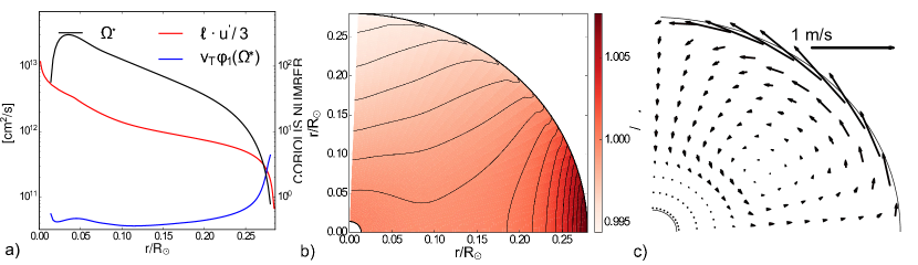
Figure 1: a) The Coriolis number $\Omega^{*}=2\tau_{c}\Omega_{\star}$ (black line), where $\tau_{c}$ is the turn-over time of convection (from the MESA code), the turbulent diffusivity parameter, red line; the blue line show isotropic eddy viscosity from the heat transport model; b) angular velocity profiles with contour levels which cover the range of values depicted on the color bar; c) geometry of the meridional circulation, in the Northern hemisphere.

Figure (1) shows profiles of the internal parameters of the mean-field model of the heat transport and the angular momentum balance together with some input parameters from the MESA code. It is found that the convective turnover time varies from about of 1 day at the near-surface layer to about of 200 days near the center of the star. This results to the strong modifications of the turbulent viscosity parameters. The resulted differential rotation is rather weak, it is about of 0.01$\Omega_{\star}$, where $\Omega_{\star}=7.25\cdot 10^{-6}$rad/s is the stellar rotation rate. The given angular velocity profile corresponds qualitatively to results of Kitchatinov et al. (2014). The angular velocity profile shows conical isolines pattern in the bulk of the star. This pattern changes to the cylinder like pattern in the equatorial region. In the portion of the star which occupied by the weakly varying angular velocity, the given pattern is different to results of the direct numerical simulations (cf, Browning 2008; Yadav et al. 2015). However, the strong shear in equatorial region is presented in all models. The meridional circulation consists of the one cell in each hemisphere with poleward flow in upper part of the star. The amplitude of the flow is about one meter per second at the surface.

2.2 Dynamo model

The dynamo model takes into account both the axisymmetric and the non-axisymmetric large-scale magnetic field. Its evolution is described by the mean-field induction equation (Krause & Rädler, 1980):

$$\partial_{t}\left\langle\mathbf{B}\right\rangle=\bm{\nabla}\times\left(\bm{\mathcal{E}}+\left\langle\mathbf{U}\right\rangle\times\left\langle\mathbf{B}\right\rangle\right)$$ (7)

where $\bm{\mathcal{E}}=\left\langle\mathbf{u\times b}\right\rangle$ is the mean electromotive force; $\mathbf{u}$ and $\mathbf{b}$ are the turbulent fluctuating velocity and magnetic field respectively; and $\left\langle\mathbf{U}\right\rangle$ and $\left\langle\mathbf{B}\right\rangle$ are the mean velocity and magnetic field. We remind that in the paper, the angle brackets are used for the ensemble average of the field which could contain the large-scale non-axisymmetric modes contributions as well as the axisymmetric modes of the mean field which is denoted by the over-bar. The mean flow is axisymmetric, i.e., $\left\langle\mathbf{U}\right\rangle\equiv\overline{\mathbf{U}}$, and it is determined from solution of the angular momentum balance. In the fully nonlinear case the solution of the angular momentum balance is coupled with the mean-field dynamo equations and the mean-field equation for the heat transport.

Let $\hat{\bm{\phi}}=\mathbf{e_{\phi}}$ and $\hat{\mathbf{r}}=r\mathbf{e}_{r}$ be vectors in the azimuthal and radial directions respectively, then we represent the mean magnetic field vectors as follows:

$$\left\langle\mathbf{B}\right\rangle = \overline{\mathbf{B}}+\tilde{\mathbf{B}}$$ (8)

$$\mathbf{\overline{B}} = \hat{\bm{\phi}}B+\nabla\times\left(A\hat{\bm{\phi}}\right)$$ (9)

$$\tilde{\mathbf{B}} = \bm{\nabla}\times\left(\hat{\mathbf{r}}T\right)+\bm{\nabla}\times\bm{\nabla}\times\left(\hat{\mathbf{r}}S\right),$$ (10)

where $\overline{\mathbf{B}}$ is the axisymmetric, and $\tilde{\mathbf{B}}$ is non-axisymmetric part of the large-scale magnetic field, $A$, $B$, $T$ and $S$ are scalar functions. Hereafter, the non-axisymmetric part of the mean field is denoted by the wave above the symbol.

We employ the mean electromotive force in form:

$$\mathcal{E}_{i}=\left(\alpha_{ij}+\gamma_{ij}\right)\left\langle B\right\rangle_{j}-\eta_{ijk}\nabla_{j}\left\langle B\right\rangle_{k}.$$ (11)

where symmetric tensor $\alpha_{ij}$ models the generation of magnetic field by the $\alpha$- effect; antisymmetric tensor $\gamma_{ij}$ controls the mean drift of the large-scale magnetic fields in turbulent medium, including the magnetic buoyancy; tensor $\eta_{ijk}$ governs the turbulent diffusion. Some details about the $\bm{\mathcal{E}}$ are given in appendix, (also, see, Pipin 2008).

In our model the $\alpha$ effect takes into account the kinetic and magnetic helicities in the following form:

$$\alpha_{ij} = C_{\alpha}\psi_{\alpha}(\beta)\alpha_{ij}^{(H)}\eta_{T}+\alpha_{ij}^{(M)}\frac{\left\langle\chi\right\rangle\tau_{c}}{4\pi\overline{\rho}\ell^{2}}$$ (12)

where $C_{\alpha}$ is a free parameter which controls the strength of the $\alpha$- effect due to turbulent kinetic helicity; $\alpha_{ij}^{(H)}$ and $\alpha_{ij}^{(M)}$ express the kinetic and magnetic helicity parts of the $\alpha$-effect, respectively; $\eta_{T}=\nu_{T}/Pm_{T}$ is the magnetic diffusion coefficient, $Pm_{T}$ is the turbulent magnetic Prandtl number and $\left\langle\chi\right\rangle=\left\langle\mathbf{a}\cdot\mathbf{b}\right\rangle$ ($\mathbf{a}$ and $\mathbf{b}$ are the fluctuating parts of magnetic field vector-potential and magnetic field vector). Both the $\alpha_{ij}^{(H)}$ and $\alpha_{ij}^{(M)}$ depend on the Coriolis number. Function $\psi_{\alpha}(\beta)$ controls the so-called “algebraic” quenching of the $\alpha$- effect where $\beta=\left\langle\left|\mathbf{B}\right|\right\rangle/\sqrt{4\pi\overline{\rho}u^{\prime 2}}$, $u^{\prime}$ is the RMS of the convective velocity.

The magnetic helicity conservation results to the dynamical quenching of the dynamo. Contribution of the magnetic helicity to the $\alpha$-effect is expressed by the second term in Eq.(12). The magnetic helicity density of turbulent field, $\left\langle\chi\right\rangle=\left\langle\mathbf{a}\cdot\mathbf{b}\right\rangle$, is governed by the conservation law (Pipin et al., 2013):

$$\frac{\partial\left\langle\chi\right\rangle^{(tot)}}{\partial t}=-\frac{\left\langle\chi\right\rangle}{R_{m}\tau_{c}}-2\eta\left\langle\mathbf{B}\right\rangle\cdot\left\langle\mathbf{J}\right\rangle-\bm{\nabla\cdot\mathcal{F}}{}^{\chi},$$ (13)

where $\left\langle\chi\right\rangle^{(tot)}=\left\langle\chi\right\rangle+\left\langle\mathbf{A}\right\rangle\cdot\left\langle\mathbf{B}\right\rangle$ is the total magnetic helicity density of the mean and turbulent fields, $\bm{\mathcal{F}}^{\chi}=-\eta_{\chi}\bm{\nabla}\left\langle\chi\right\rangle$ is the diffusive flux of the turbulent magnetic helicity, and $R_{m}$ is the magnetic Reynolds number. The coefficient of the turbulent helicity diffusivity, $\eta_{\chi}$, is chosen ten times smaller than the isotropic part of the magnetic diffusivity , $\eta_{\chi}=\frac{1}{10}\eta_{T}$. The magnetic helicity conservation is determined by the magnetic Reynolds number $R_{m}$. In this paper we employ $R_{m}=10^{4}$.

The numerical scheme employs the spherical harmonics decomposition for the non-axisymmetric part of the problem. At the bottom of the domain we put the potentials $S$ and $T$ , as well as the axisymmetric fields, $B$ and $A$ to zero. At the top the poloidal field is smoothly matched to the external potential field and the toroidal field goes to zero

The numerical scheme employs the pseudo-spectral approach for integration along latitude and the finite differences along the radius. Fort the non-axisymmetric part of the problem we employ the spherical harmonics decomposition, i.e., the scalar functions $T$ and $S$ are represented in the form:

$$T\left(r,\mu,\phi,t\right) = \sum\hat{T}_{l,m}\left(r,t\right)\bar{P}_{l}^{\left|m\right|}\exp\left(im\phi\right),$$ (14)

$$S\left(r,\mu,\phi,t\right) = \sum\hat{S}_{l,m}\left(r,t\right)\bar{P}_{l}^{\left|m\right|}\exp\left(im\phi\right),$$ (15)

where $\bar{P}_{l}^{m}$ is the normalized associated Legendre function of degree $l\geq 1$ and order $m\geq 1$. The simulations which we will discuss include 310 spherical harmonics (up to $l_{max}=20$). Note that $\hat{S}_{l,-m}=\hat{S}_{l,m}^{*}$ and the same for $\hat{T}$. All the nonlinear terms are treated explicitly in the real space. The numerical integration is carried out in latitude from the pole to pole and in radius from $r_{b}=0.05R_{\star}$ to $r_{e}=0.98R_{\star}$.

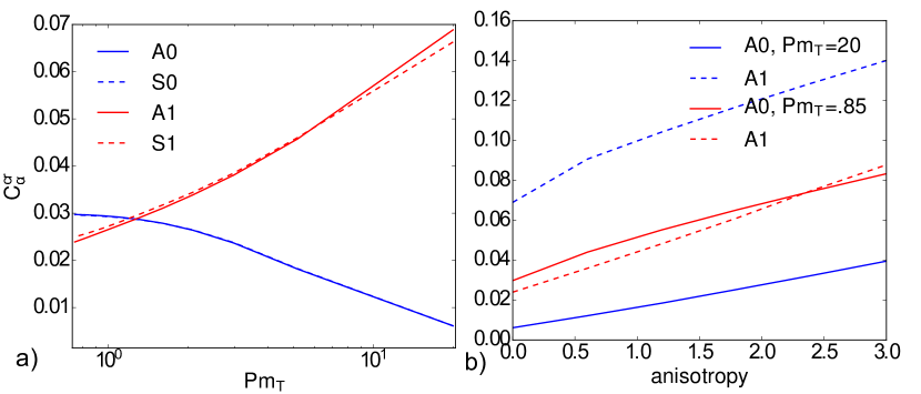
Figure 2: The critical threshold parameter $C_{\alpha}^{(cr)}$ for isotropic diffusivity, $A=0$; b) The dependence of the critical threshold parameter $C_{\alpha}^{(cr)}$ on the anisotropy of the turbulent diffusivity, for $Pm_{T}=20$ (blue lines), and $Pm_{T}=0.85$, (red lines).

The thermal equilibrium, the angular momentum balance and evolution of the large-scale magnetic field is controlled by the free parameters, which are the angular velocity of the global rotation $\Omega_{0}=7.25\times 10^{-6}{\rm rad/s}$, the turbulent Prandtl number $Pr_{T}={\displaystyle\frac{\nu_{T}}{\chi_{T}}}$, the turbulent magnetic Prandtl number $Pm{}_{T}={\displaystyle\frac{\nu_{T}}{\eta_{T}}}$ , the parameter of the magnetic field generation by the $\alpha$-effect, $C_{\alpha}$, and the magnetic Reynolds number $R_{m}$. We use the mixing-length expression for the eddy heat conductivity, ${\displaystyle\chi_{T}=\frac{\ell^{2}}{6}\sqrt{-\frac{g}{c_{p}}\frac{\partial\overline{s}}{\partial r}}}.$ In the all models we fix $Pr_{T}={\displaystyle{\displaystyle\frac{3}{4}}}$, $Pm{}_{T}=3$, and $R_{m}=10^{4}$. We will discuss the possible dependence of results on $Pm_{T}$ , as well.

We studied the eigenvalue dynamo problem before running the nonlinear models. In the linear model we neglect the radial dependence of the $\alpha$-effect and turbulent diffusivity. Solutions of the eigenvalue problem showed that the linear properties of the dynamo model are in agreement with results reported earlier by Elstner & Rüdiger (2007) and Shulyak et al. (2015). More specifically, the results of the linear problem solutions are as follows. Firstly, for the high $Pm_{T}$ the axisymmetric dynamo has smaller the critical dynamo instability threshold instability than the non-axisymmetric dynamo. The transition from axisymmetric to non-axisymmetric regimes occurs for $Pm_{T}\approx 1$. This is in agreement with findings of Shulyak et al. (2015). Also the solution shows that the critical threshold for the symmetric and antisymmetric about equator dynamo modes are close and the symmetric modes have the smaller threshold than the antisymmetric ones. Secondly, it was found that for the case $Pm_{T}\approx 1$, when the non-axisymmetric dynamo instability is more powerful than the axisymmetric one, the rotationally induced anisotropy of the magnetic diffusivity can promotes the dynamo instability of the axisymmetric magnetic field if the amplitude of the eddy diffusivity along the rotation axis is twice of that one in the perpendicular direction. This result is in agreement with that reported by Elstner & Rüdiger (2007). Figures 2(a,b) illustrate our findings. In comparing our results with findings from reported in above cited papers we have to take into account that the parameter of the $\alpha$-effect in the reduced linear models contain the density stratification factor, $\bm{\tilde{\Lambda}}^{(\rho)}=R_{\odot}\bm{\nabla}\log\overline{\rho}$, and its mean value in the star is $\overline{\left|\bm{\tilde{\Lambda}}^{(\rho)}\right|}\approx 50$. Also models of Shulyak et al. (2015) were normalized for diffusivity $10^{11}\mathrm{cm^{2}/s}$ and it is $10^{13}\mathrm{cm^{2}/s}$ in our model.

Table 1: Basic parameters, $B_{max}$ is the maximum of the magnetic field strength in the star, $\overline{B}_{\|}$ and $\tilde{B}_{\|}$ are the mean strength of the mean poloidal components of the axisymmetric and non-axisymmetric magnetic field at the surface, $\overline{B}_{\perp}$ and $\tilde{B}_{\perp}$ is the same for the toroidal magnetic field below surface at the ${\displaystyle\frac{3}{4}}R_{\star}$, M is the ratio of the energy of the non-axisymmetric magnetic field to the total magnetic energy at the same radial distance and ${\displaystyle\overline{\frac{\Delta\Omega}{\Omega}}}$ is the measure of the latitudinal shear at the surface.

	$C_{\alpha}$	Angular Momentum	$B_{max}$, [kG]	$\overline{B}_{\|}$, $\tilde{B}_{\|}$ [kG]	$\overline{B}_{\perp}$,$\tilde{B}_{\perp}$ [kG]	$M={\displaystyle\frac{\tilde{E}_{m}}{E_{m}}}$	${\displaystyle\overline{\frac{\Delta\Omega}{\Omega}}}$
M1	0.04	no	3	0.3, 0	1.5, 0	0	0.014
M2	0.04	no	4	0.2, 0.35	1, 2	0.5	0.014
M3	0.05	no	8	0.04, 0.8	0.2, 4	0.9	0.014
M4	0.04	yes	1.5	0.2	0.35	0	0.012
M5	0.05	yes	1.8	0.2,0.3	0.7,1	0.6	0.009

3 Results

Table 1 contains general parameters of our models. They are: the $B_{max}$ is the maximum strength of the large-scale magnetic field in the star, the $\overline{B}_{\|}$ and $\tilde{B}_{\|}$ are the mean strength of the axisymmetric and non-axisymmetric large-scale poloidal magnetic field on the surface, the $\overline{B}_{\perp}$ and $\tilde{B}_{\perp}$ is the same for the toroidal magnetic field at the radial distance ${\displaystyle\frac{3}{4}}R_{\star}$, the $M={\displaystyle\frac{\tilde{E}_{m}}{E_{m}}}$ is the ratio of the energy of the non-axisymmetric mode of the large-scale magnetic field to the total magnetic energy of the large-scale field at the radial distance ${\displaystyle\frac{3}{4}}R_{\star}$, and the parameter ${\displaystyle\overline{\frac{\Delta\Omega}{\Omega}}}$ is the mean latitudinal shear on the top of the integration domain, where the mean is computed over one dynamo cycle.

In the paper we show results for five different runs of the nonlinear dynamo models. In all the runs we put $Pm_{T}=3$. In this case the dynamo period is about 40 years. Shulyak et al. (2015) discussed linear dynamo regimes with the longer dynamo period about 100Y. This is because they employed the higher $Pm_{T}=10$ in thier models. We have nonlinear runs with $Pm_{T}=10$ but not for all cases listed in the Table 1. The higher $Pm_{T}$, the longer dynamo period and it takes longer evolution time for the model to reach some stationary regime of the dynamo oscillations, especially in the case of the non-axisymmetric dynamo regimes. Also the effect of the meridional circulation for the case of $Pm_{T}=10$ requires the better spatial resolution near poles. We made separate runs for axisymmetric and non-axisymmetric dynamo regimes. The latter models take into account both the axisymmetric and non-axisymmetric magnetic field generation. In this paper we restrict the study of the fully nonlinear model by the case of the $C_{\alpha}$ when both the axisymmetric and the non-axisymmetric magnetic fields are unstable to generation in the large-scale dynamo. The initial field in all runs has no preferable parity relative to the equator.

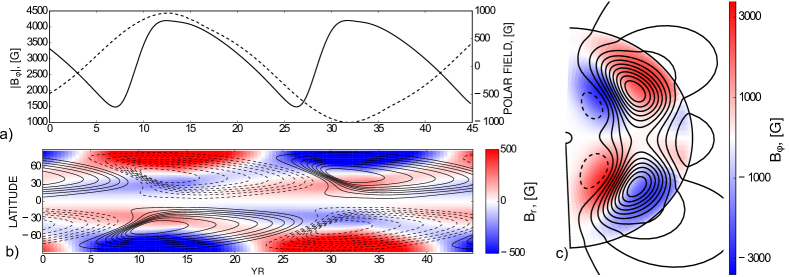
Figure 3: The model M1, a) evolution of the mean strength toroidal magnetic field at the $r=\frac{3}{4}R_{\star}$and the radial magnetic field strength at the North pole (dashed line); b) the time-latitude diagram for toroidal magnetic field (contours in range $\pm 4$kG) at the $r=\frac{3}{4}R_{\star}$, and the color image shows the radial magnetic field at the surface; c) snapshot of the large-scale magnetic field distributions at the growing phase of the cycle

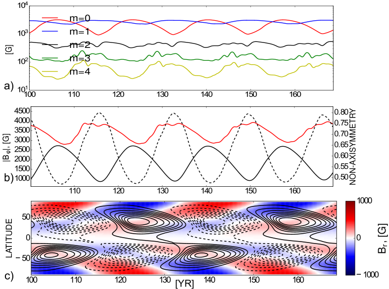
Figure 4: The model M2, a) the mean strength of the first five partial modes of the toroidal magnetic field at the $r=\frac{3}{4}R_{\star}$; b) at the same $r$, the index of the non-axisymmetric of the large-scale magnetic field (dashed line), the mean strength of the axisymmetric toroidal magnetic field (solid line) and the mean strength of the large-scale toroidal field taking into account both the axisymmetric and non-axisymmetric parts of the magnetic field; c) the same as Fig.3b

3.1 Nonlinear $\alpha$-effect

In this subsection we consider the nonlinear models with magnetic feedback on the generation of the large-scale magnetic fields by the $\alpha$-effect. The models remain kinematic relative to the large-scale flow. The non-linear $\alpha$-effect takes into account the dynamical feedback due to magnetic helicity conservation (see, the Eq(13)) and the “instantaneous” quenching which is related with magnetic feedback from the Lorentz forces on the turbulent convection. This concept was originally formulated by Kleeorin & Ruzmaikin (1982). The Fig.3 show results for the model M1 which illustrates the axisymmetric dynamo when the parameter of the parameter $C_{\alpha}$ is about factor one and half of the critical dynamo instability threshold. The model show the mixed parity solution with some preference to generation of the antisymmetric about equator magnetic field. Butterfly diagrams shows the solar-like equatorial drift of the toroidal magnetic field of the strength 4kG at the $r=\frac{3}{4}R_{\star}$. The radial magnetic field drift to the pole where it reaches strength of the 1kG during the maximum of the dynamo cycle. The polar drift of the poloidal field is supported by the meridional circulation. The migrating dynamo wave of the poloidal magnetic field is transformed to the steady one when the meridional circulation is neglected. Also, in this case the dominance of the antisymmetric relative to equator magnetic field become less clear in the nonlinear mixed parity solution. It is found that the meridional flow has only a small effect on the amplitude of the dynamo wave.

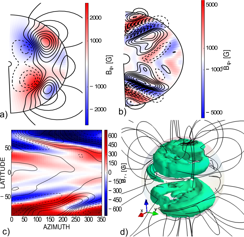
Figure 5: The model M2, a) snapshot of the axisymmetric toroidal magnetic field (color image) and the poloidal field at the end of run ($t=170$ Yr); b) snapshot of distribution the non-axisymmetric magnetic field at the longitude $\phi=0$ , color image shows the toroidal magnetic field and contours - the poloidal magnetic field; c) the non-axisymmetric radial magnetic field at the surface (color image) and contours show the toroidal field at the subsurface layer; d) magnetic field lines out of the star and surface show the large-scale magnetic field of magnitude 1kG inside the star.

Results of the linear problem study show that the non-axisymmetric magnetic field is unstable to generation for the same parameter $C_{\alpha}$ as it is employed in the model M1. The model M2 takes the non-axisymmetric magnetic field into account. Fig.4 show results for variations of the magnetic energy, index of the non-axisymmetric and the time-latitude diagrams of the axisymmetric magnetic field in the model. We find that the non-axisymmetric dynamo quenches the strength of the generated axisymmetric magnetic field. The most important quenching mechanisms are due to effects of the magnetic helicity generation from the non-axisymmetric dynamo and another effect is due to the magnetic buoyancy which is increased when the magnetic energy increases. In our intepretation, we have to take into account that the magnetic buoyancy can promote the dynamo instability of the non-axisymmetric field (Dikpati & Gilman, 2001).

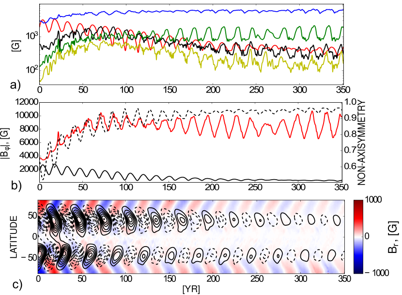
Figure 6: The same as the Figure 4 for the model M2.

The non-axisymmetric dynamo wave has a spiral pattern which is rigidly rotating (see Fig 5d), which produces Yin Yang magnetic polarity pattern on the surface of the star. The strength of the spiral arms vary in time because of interaction with the axisymmetric magnetic field. This causes the long-term variation of the magnetic energy of the non-axisymmetric field at the given radial distance of the star.

Figure 5 show snapshots of the magnetic field distribution inside and outside of the star. Configuration of the axisymmetric field in the model M2 is similar that in the model M1. The non-axisymmetric field is distributed along iso-surface of the angular velocity. The polar regions on the surface of star are occupied by the mixture of the axisymmetric radial magnetic and the non-axisymmetric field magnetic field of the m=1 mode.

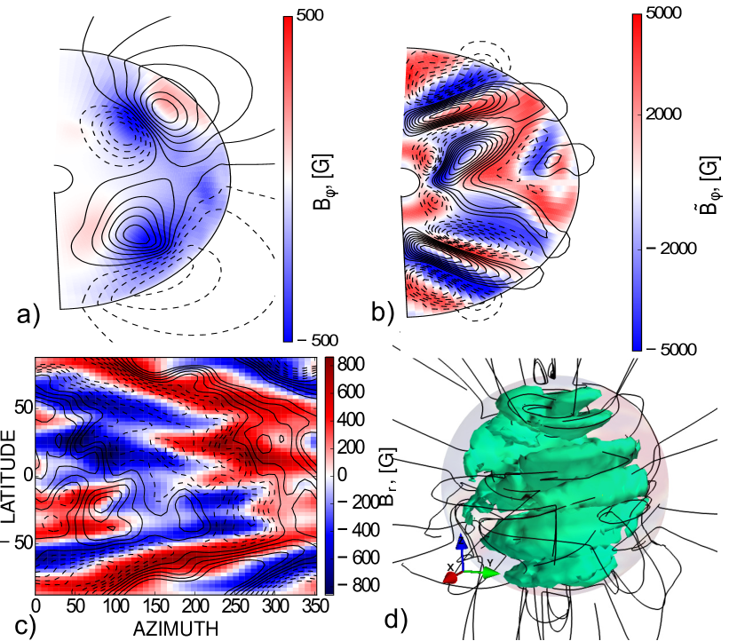
Figure 7: The same as the Figure 5 for the model M3

In the model M3 the alpha-effect parameter $C_{\alpha}$ is about twice of the dynamo instability threshold. The model M3 shows the stronger quenching of the axisymmetric dynamo than the model M2. This is illustrated in Figures 6 and 7. In fact, the axisymmetric magnetic field nearly disappear in the stationary phase of the evolution. At the surface the non-axisymmetric magnetic field shows the large-scale spot-like pattern with angular size about 30^∘. Those spots are located in the equatorrial and polar regions as well.

3.2 Fully non-linear dynamo

This subsection contain results about the fully nonlinear dynamo with regards for the magnetic feedback on the angular momentum balance and heat transport inside the star. In the model M4 we neglect effects of the non-axisymmetric field on the dynamo.

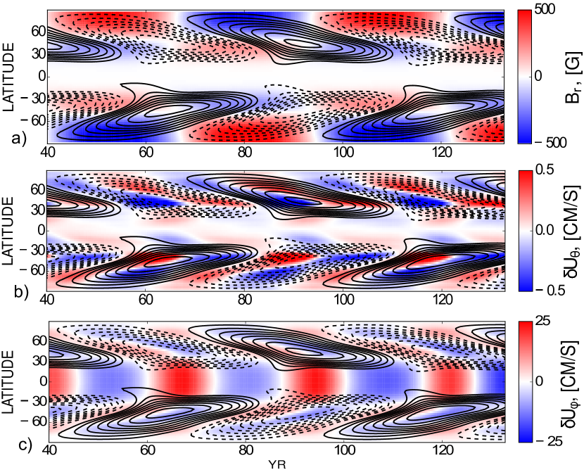
Figure 8: The model M4, a) the time-latitude diagram for toroidal magnetic field (contours in range $\pm 1.5$kG) at the $r=\frac{3}{4}R_{\star}$, and the color image shows the radial magnetic field at the surface; b) color image show the variation of the latitudinal meridional flow (positive to the equator) c) the same as b) for variation of the toroidal velocity field at the surface;

Figure 8 show the time-latitude diagrams for variations of the magnetic field, angular velocity and the latitudinal component of the meridional flow in the model M4. The variations of the angular velocity caused by the dynamo, can be observed as the azimuthal flow waves. The model M4 demonstrate some similarity to the solar case, i.e., the positive azimuthal flow wave is located on the equatorial side of the dynamo wave of the large-scale toroidal field. Simultaneously, the model shows the meridional flows direct to the maximum of the toroidal magnetic field. Zonal variations of rotation is about 10 percents of the mean latitudinal shear. Variations of the meridional circulation are smaller than one percent of the mean magnitude. The surface mean latitudinal shear in model M4 is about 15 percents smaller than in the kinematic models. Magnetic feedback on the differential rotations reduces the strength of the toroidal field in the model by factor 3 in compare to model M1.

Figure 9 show variations of the magnetic field and angular velocity on period of half of the magnetic cycle. It is seen that dynamo wave migrate outward of the rotation axis. The migration of the dynamo waves induces variations of the angular velocity which is separated to zones of the accelerated and decelerated motions. Those zones are elongated along the rotation axis. The dynamo wave inside star distorts distribution of the angular velocity bowing the angular velocity iso-surface to equator. It makes the angular velocity profile inside the star to become close to the spherical surfaces. This supports the equatorial drift of the dynamo wave. In the upper part of the star drift of the dynamo waves of the toroidal field follows the distorted isolines of the angular velocity. The drift goes equator-ward up to 30^∘ latitude. The drifting wave of the poloidal field is transformed to nearly steady on the surface because of effect of the meridional circulation. We also see that rather small variations of the meridional circulation are concentrated to the surface.

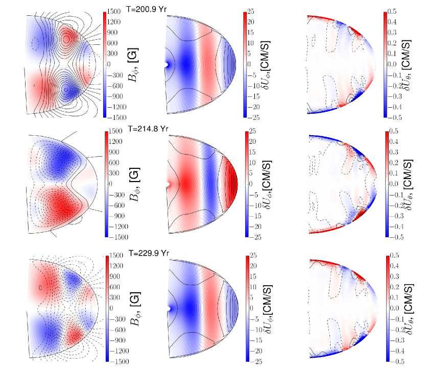
Figure 9: Model M4. Snapshots of the magnetic field (left), angular velocity, the azimuthal zonal flow distributions (middle) and the meridional circulation (right, color image is for the latitudinal component and contours are for the radial component) for a half of the dynamo cycle.

The reduced differential rotation results to a reduced ratio between the mean strength of the toroidal and poloidal field. In the model M4 it is about 2 and in the models M1, M2, M3 it is about 5. The strength of the polar field in the model M4 is about 500 G which is by factor 2 smaller than in models M1 and M2.

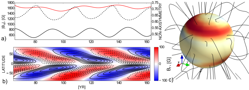
Figure 10: The model M5, a) the mean strength of sum the first five partial modes of the toroidal magnetic field at the $r=\frac{3}{4}R_{\star}$ (red line), the index of the non-axisymmetric of the large-scale magnetic field (dashed line), the mean strength of the axisymmetric toroidal magnetic field (solid black line); b) the time-latitude diagram of the axisymmetric toroidal magnetic field at the $r=\frac{3}{4}R_{\star}$ (contours for the range $\pm 500$G) and the axisymmetric radial magnetic field at the surface; c) snapshot of the large-scale magnetic field lines out of the star and the backgorund image shows the radial magnetic field within range of $\pm 300$G.

Compare to the previous case, the model M5 takes into account effects of the non-axisymmetric field in the angular momentum balance via the mean Maxwell stresses of the non-axisymmetric magnetic field, i.e., terms like ${\displaystyle-\frac{\overline{\tilde{B}_{i}\tilde{B}_{j}}}{4\pi\overline{\rho}}}$ (over-bar means the azimuthal averaging) and contributions of the non-axisymmetric field to the mean magnetic energy. The latter makes effect to the efficiency of the magnetic quenching of the $\Lambda$ effect and coefficients of the eddy viscosity and thermal eddy conductivity. Figure 10 shows evolutions of parameters of the large-scale magnetic field and snapshot for the magnetic field distribution out of the star. It is found that the non-axisymmetric dynamo quenches generation of the axisymmetric magnetic field. However, unlike to the model M3, which has the same parameter $C_{\alpha}$, the axisymmetric dynamo persists in the stationary stage of evolution of the model M5. This is similar to the model M2. The dynamo wave goes equator-ward in the whole range of latitudes. The surface magnetic field is dominated by the m=1 mode of the non-axisymmetric magnetic field with the Yin Yang magnetic polarity pattern as well as the model M2.

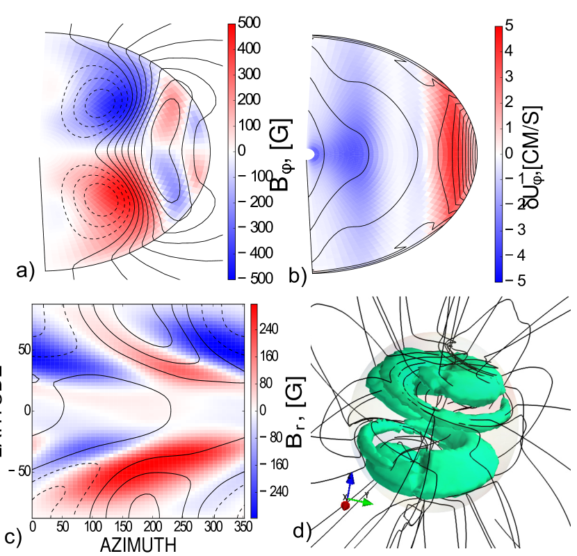
Figure 11: Except the panel b) the same as Figure 5 for the model M5. The panel b) shows, the distribution of the mean angular velocity (contours), and the background image shows distribution of the zonal variations of rotation.

Figure 11 shows snapshots of the magnetic field and angular velocity distributions in the star for the model M5. The snapshot of the axisymmetric magnetic field is similar to those demonstrated in the other models. The magnetic field is antisymmetric about equator showing three bands of the toroidal magnetic field propagating outward of the rotation axis, along the spherical iso-surfaces of the angular velocity (see, Figure 11b). The zonal variations of the angular velocity are small and their patterns are elongated along the axis of rotation. Similar to models M2 and M3, the large-scale magnetic field inside the star has a spiral structure because the non-axisymmetric mode m=1 dominates the others partial modes.

In our simulations, we also have tried the larger values of the parameters $Pm_{T}$ and $C_{\alpha}$. Results for the kinematic models with non-linear $\alpha$ effect and $Pm_{T}=10$ are similar the model M3. The period of the axisymmetric dynamo in case of $Pm_{T}=10$ is about 120 years in agreement with expectations of Shulyak et al. (2015). The model show rather strong polar axisymmetric magnetic field with the strength of 1.5kG. This is because of the meridional circulation effect. Its efficiency ncreases with the increase of the parameter $Pm_{T}$. For the $Pm_{T}=10$ the axisymmetric regime persists when the $C_{\alpha}<0.04$. We found the transition to the non-axisymmetric dynamo for the $C_{\alpha}=0.05$. The properties of the non-axisymmetric mean-field dynamo in the fully non-linear regime for the case of $Pm_{T}=10$ remain unclear.

4 Discussion

The previous consideration of the mean-field models of the fully convective stars was restricted to analysis of the eigenvalue problems (Elstner & Rüdiger, 2007; Shulyak et al., 2015) or the kinematic case with uniform density stratification and the algebraic non-linearity of the $\alpha$-effect (Chabrier & Küker, 2006). The main progress in theoretical understanding of the dynamo on the the fully convective stars were made with help of the direct numerical simulations (see, e.g., Dobler et al. 2006; Browning 2008; Gastine et al. 2012; Yadav et al. 2015). The paper for the first time presents results of the non-linear mean-field dynamo models of the fully convective star rotating with period 10 days.

The key reasons to study the mean-field models is to study behavior of the dynamo in varying the governing dynamo parameters. At the first step, let us discuss the kinematic dynamos with the nonlinear $\alpha$-effect. The angular velocity profile in this case is different to the cylinder-like pattern, which was discussed in the literature (see, e.g., Moss 2004, 2005; Chabrier & Küker 2006) and which appears in the direct numerical simulations. Our model include effect of the meridional circulation which is important in the subsurface layer for the case of $Pm_{T}>1$. For the case $Pm_{T}=3$, the model M1 shows the strong axisymmetric dipole-like magnetic field with magnitude of the polar field about 1kG. The dominance of the antisymmetric relative to equator magnetic field disappears in the nonlinear mixed parity solution if we neglect the meridional circulation. The dynamo waves show the solar-like time-latitude diagrams with toroidal field drifting to the equator and the radial field drifting to the pole.

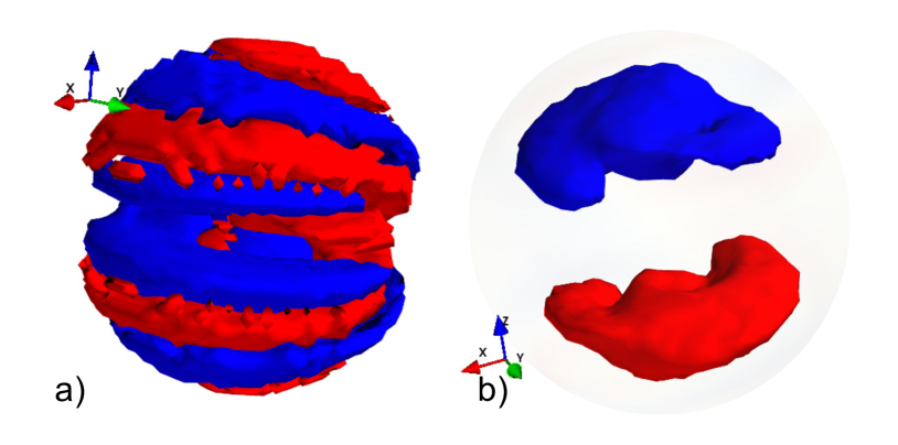
Figure 12: Snapshots of the model M5, a) the nonlinear $\alpha$ effects (volume contours for $\pm$3cm/s); b) the small-scale magnetic helicity density (from the Eq(13)), (volume contours for $\pm$1.05$\cdot 10^{10}$G²/M)

The eigenvalue analysis shows that generation of the non-axisymmetric magnetic field for the case of $Pm_{T}>1$ is less efficient than the axisymmetric dynamo because the critical parameter of the dynamo instability is smaller in the second case. This is general conclusion of the most studies of the mean field dynamo starting from the seminal paper by Raedler (1986). The conclusion lead to ignorance of the non-axisymmetric dynamos even for the super-critical regimes of the axisymmetric dynamo (cf, Raynaud & Tobias 2016). However the model M2 show that in case of the dynamo instability of the non-axisymmetric field, the non-axisymmetric regime can beat the axisymmetric one. The interaction between axisymmetric and non-axisymmetric magnetic field goes via the nonlinear effects. Those are the conservation of the magnetic helicity and the magnetic buoyancy. Contributions of the magnetic helicity on the $\alpha$-effect can not be ignored in the mean-field solar dynamos (Brandenburg & Käpylä, 2007). They are important in the non-axisymmetric dynamo, as well. The change of the dynamo regime for the overcritical $C_{\alpha}$ is because of the non-axisymmetric $\alpha$-effect, which is produced by the magnetic helicity conservation in the non-axisymmetric large-scale dynamo. Figures12(a,b) show snapshots of the $\alpha_{\phi\phi}$ (see, Eq.(12) and the mean magnetic helicity density of the small-scale field, which is generated because of the magnetic helicity conservation in the model M5. Models M2 and M3 show similar distributions. The models produce the non-axisymmetric non-linear $\alpha$ effect and this supports dominance the non-axisymmetric magnetic field in the dynamo. In the solar dynamo models the non-axisymmetric $\alpha$-effect was employed for explanation of the so-called active longitudes of the sunspot formations (Bigazzi & Ruzmaikin, 2004; Berdyugina et al., 2006). In our models this effect stems naturally from magnetic helicity conservation.

The magnetic feedback on the differential rotation reduces efficiency of the axisymmetric dynamo. The strength of the large-scale magnetic field in the model M4 is less than in the model M1. The cyclic effect of the large and small-scale Lorentz force on the angular momentum fluxes produces phenomena known in the solar magnetic acitvity like the zonal variations of the angular velocity and variations of the meridional flow. Both of them predicted to have much smaller amplitude than for the Sun. The rotational velocity at the equator is $1.44$ km/s, then the predicted magnitude of the latitudinal shear between equator and pole is only about 14 m/s. Therefore our models demonstrate the dynamo induced zonal variations are about of 10 percent of magnitude of the mean latitudinal shear. The relative variations of the meridional circulation are about 1 percent of the mean flow which is much smaller than it is observed on the Sun. Note, the M-dwarf has much denser plasma than the Sun and for the 1kG magnetic field at the top of the integration domain ($0.98R_{\star}$) the Alfven velocity is less than $6$m/s. In the model the toroidal field does not penetrate to the surface because of the vacuum boundary conditions and this reduces the magnitude of the large-scale flow variations on the surface. Unlike the Sun (see, eg, Birch 2011; Howe et al. 2011; Kosovichev et al. 2013) the predicted torsional oscillations have the equal magnitudes in the bulk of the star and at the surface. Variations of the meridional circulation are concentrated to the surface. Note , that the radial profile of the meridional circulation is still unclear in the case of the Sun, see preliminary results in the papers by Hathaway (2012) and Zhao et al. (2013), who supports concentration of 11-th year variations of the solar meridional circulation to the surface.

It is predicted that magnetic activity produces rather strong distortion of the angular velocity profile inside the star leaving the structure of the meridional flow nearly the same as it is in the kinematic models. The same results were found in the direct numerical simulations of Browning (2008) and Yadav et al. (2015). Figure 13a allows comparison to their results. We find that in the magnetic case (the model M5) the latitudinal shear persists only in the upper layer of the star. Also, there the strong radial shear presents near the equator. The same was found in the direct numerical simulation by Yadav et al. (2015). The model of Browning (2008) showed the uniform angular velocity profile in the magnetic case. We find that in the nonlinear model M5 the positive radial shear in the equatorial region is stronger than in the kinematic model M1. Also we see formation of the radial shear at the surface in the polar region in the model M5. The increase of the magnitude of the subsurface shear as a result of the magnetic field influence on the angular momentum fluxes is also in agreement with the recent numerical simulations on the solar-like stars (Guerrero et al. 2013; Käpylä et al. 2014; Guerrero et al. 2016).

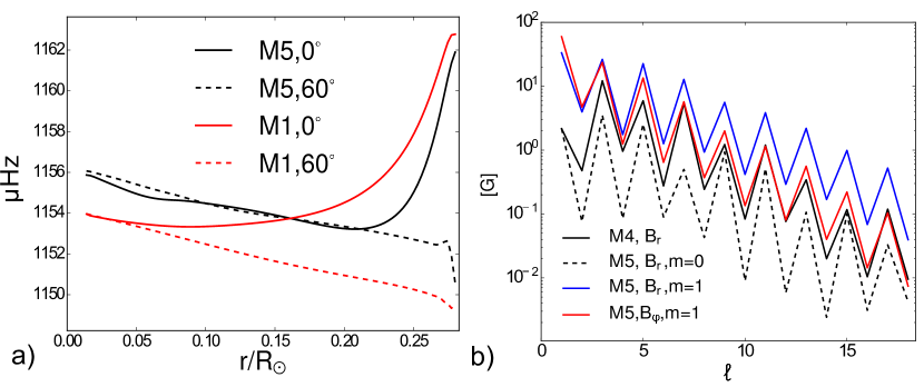
Figure 13: a) The angular velocity radial profile in the kinematic (red lines) and nonlinear models M1 and M5 for the equator ($0^{\circ}$) and 60^∘ latitudes; b)Modes.

Our results show that the strength of the surface poloidal magnetic field is only factor two or three lesser than the strength of the toroidal magnetic field inside the star, see the Table 1. All the models show rather strong polar magnetic field, 1kG in the kinematic models and from 100 to 500 G in the nonlinear models. Current observations of the stellar magnetic activity inform us a lot about the topological and spectral properties of the magnetic field distributions at M-dwarfs and cool stars (Morin et al., 2010; See et al., 2016). Figure 13b presents results of the spherical harmonic decomposition for magnetic field predicted by the fully nonlinear models M4 (axisymmetric one) and M5. In the axisymmetric model M4 we don’t expect any toroidal field out of the surface because of the boundary conditions. In this case the energy of the magnetic field outside the star is dominated by $\ell=3$ and $\ell=5$ harmonics which is similar to the Sun (Stenflo & Guedel, 1988; Stenflo, 2013; Vidotto, 2016). The non-axisymmetric dynamo model M5 show the dominance of the mode m=1 and $\ell=1$ of the large-scale toroidal magnetic field. The ratio of the energy of the non-axisymmetric and axisymmetric poloidal magnetic field in the model M5 is about factor order of the magnitude. The given results are in agreement with Morin et al. (2010) for the magnetic field observations for the early types of the M-dwarfs with a moderate rotation rates.

Let’s summarize the main findings of the paper. Our study confirm the previous conclusions of Shulyak et al. (2015) that the weak differential rotation of the M-dwarfs can support the axisymmetric dynamo especially for the case $Pm_{T}>1.$ For the case $Pm_{T}=3$ we find that the generation threshold $\alpha$-effect parameter $C_{\alpha}$ is lower for axisymmetric magnetic field. However for the overcritical $\alpha$-effect the non-axisymmetric dynamo become preferable. The situation is reproduced both in the kinematic and in the fully nonlinear dynamo models. In the non-linear case the differential rotation of the star deviates strongly from the kinematic case. For the most complete non-linear dynamo model we found the non-axisymmetric magnetic field of strength about 0.5kG at at the surface mid latitude, it is rigidly rotating and it is perturbed by the axisymmetric dynamo waves propagating out of the rotational axis. The predicted dynamo period of the axisymmetric dynamo waves in the model is about 40 Yr for the $Pm_{T}=3$ and it is longer for the higher $Pm_{T}$.

Acknowledgements

I appreciate Prof D.D. Sokoloff, Prof D. Moss and Dr D.Shulyak for discussions and comments. I thank the financial support of the project II.16.3.1 of ISTP SB RAS and the partial support of the RFBR grants 15-02-01407-a, 16-52-50077-jaf.

5 Appendix

5.1 Heat transport

Pipin (2004) found that under the joint action of the Coriolis force and the large-scale toroidal magnetic field, and when it holds $\Omega^{*}>1$, the eddy heat conductivity tensor could be approximated as follows

$$\chi_{ij}\approx\chi_{T}\left(\phi_{\chi}^{(I)}\left(\beta\right)\phi\left(\Omega^{*}\right)\delta_{ij}+\phi_{\chi}^{(\|)}\left(\beta\right)\phi_{\parallel}\left(\Omega^{*}\right)\frac{\Omega_{i}\Omega_{j}}{\Omega^{2}}\right),$$ (A1)

where

$$\phi_{\chi}^{(I)} = \frac{2}{\beta^{2}}\left(1-\frac{1}{\sqrt{1+\beta^{2}}}\right),$$

$$\phi_{\chi}^{(\|)} = \frac{2}{\beta^{2}}\left(\sqrt{1+\beta^{2}}-1\right).$$

Expression A1 were obtained the standard schemes of the mean-field magnetohydrodynamics employing the so-called “second order correlation approximation” and the mixing length approximations. Also we skip components of the tensor along the large-scale magnetic field.

The heat transport by radiation reads,

$$\mathbf{F}^{rad}=-c_{p}\overline{\rho}\chi_{D}\bm{\nabla}T,$$

where

$$\chi_{D}=\frac{16\sigma\overline{T}^{3}}{3\kappa\overline{\rho}^{2}c_{p}},$$

where $\kappa$ is opacity coefficient. The radial profiles of the gravity acceleration, $g$, the density, $\overline{\rho}$, the temperature, $\overline{T}$, the heat source, $\epsilon$, as well as others thermodynamic parameters, like the $c_{p}$ or the $\kappa$ are taken form the reference model which was calculated with help of the MESA code.

5.2 Angular momentum balance

Expression of the Reynolds is determined from the mean-field hydrodynamics theory (see, Kitchatinov et al. 1994; Kitchatinov 2004) as follows

$$\hat{T}_{ij}=\left(\left\langle u_{i}u_{j}\right\rangle-\frac{1}{4\pi\overline{\rho}}\left(\left\langle b_{i}b_{j}\right\rangle-\frac{1}{2}\delta_{ij}\left\langle\mathbf{b}^{2}\right\rangle\right)\right),$$ (A2)

where $\mathbf{u}$ and $\mathbf{b}$ are fluctuating velocity and magnetic fields. The turbulent stresses take into account the turbulent viscosity and generation of the large-scale shear due to the $\Lambda$- effect (Kitchatinov & Olemskoy, 2011):

$$T_{r\phi} = \overline{\rho}\nu_{T}\left\{\Phi_{\perp}+\left(\Phi_{\|}-\Phi_{\perp}\right)\mu^{2}\right\}r\frac{\partial\sin\theta\Omega}{\partial r}$$

$$+ \overline{\rho}\nu_{T}\sin\theta\left(\Phi_{\|}-\Phi_{\perp}\right)\left(1-\mu^{2}\right)\frac{\partial\Omega}{\partial\mu}$$

$$- \overline{\rho}\nu_{T}\sin\theta\Omega\left(\frac{\alpha_{MLT}}{\gamma}\right)^{2}\left(V^{(0)}+\sin^{2}\theta V^{(1)}\right),$$

$$T_{\theta\phi} = \overline{\rho}\nu_{T}\sin^{2}\theta\left\{\Phi_{\perp}+\left(\Phi_{\|}-\Phi_{\perp}\right)\sin^{2}\theta\right\}\frac{\partial\Omega}{\partial\mu}$$

$$+ \overline{\rho}\nu_{T}\left(\Phi_{\|}-\Phi_{\perp}\right)\mu\sin^{2}\theta r\frac{\partial\Omega}{\partial r}$$

$$+ \overline{\rho}\nu_{T}\mu\Omega\sin^{4}\theta\left(\frac{\alpha_{MLT}}{\gamma}\right)^{2}H^{(1)},$$

where $\nu_{T}={\displaystyle\frac{4}{5}\eta_{T}}$. The viscosity functions - $\Phi_{\|},\Phi_{\perp}$ and the $\Lambda$- effect - $V^{\left(0,1\right)}$ and $H^{\left(1\right)}$, are dependent on the Coriolis number and the strength of the large-scale magnetic field. They also depends on the anisotropy of the convective flows. Similar to the Subsection5.1 we employ the fast rotating regime of the magnetic quenching for the eddy viscosity and the the $\Lambda$- effect as it was discussed earlier in (Kueker et al., 1996; Pipin, 1999, 2004):

$$\Phi_{\perp}\!\!\! =\!\!\! \!\!\psi_{\perp}\left(\Omega^{\star}\right)\phi_{V\perp}\left(\beta\right),\,\,\Phi_{\parallel}=\psi_{\parallel}\left(\Omega^{\star}\right)\phi_{\chi}^{(I)}\left(\beta\right),$$ (A5)

$$V^{(0)}\!\!\! =\!\!\! \!\!\left(J_{0}\left(\Omega^{\star}\right)\!+\!J_{1}\left(\Omega^{\star}\right)\!+\!a\left(I_{0}\left(\Omega^{\star}\right)\!+\!I_{1}\!\left(\Omega^{\star}\right)\!\!\right)\!\right)\!\phi_{\chi}^{(I)}\!\!\left(\beta\right)\!,$$ (A6)

$$V^{(1)}\!\!\! =\!\!\! \!\!\left(J_{1}\left(\Omega^{\star}\right)+aI_{1}\left(\Omega^{\star}\right)\right)\phi_{\chi}^{(I)}\left(\beta\right),$$ (A7)

$$H^{(0)}\!\!\! =\!\!\! \!\!J_{4}\left(\Omega^{\star}\right)\phi_{H}\left(\beta\right),$$ (A8)

and $H^{(1)}=-V^{(1)}$, where the new magnetic quenching functions are:

$$\phi_{V\perp} = \frac{4}{\beta^{4}\sqrt{\left(1+\beta^{2}\right)^{3}}}\left(\left(\beta^{4}+19\beta^{2}+18\right)\sqrt{\left(1+\beta^{2}\right)}\right.$$ (A9)

$$- \left.8\beta^{4}-28\beta^{2}-18\right),$$

$$\phi_{H} = \frac{4}{\beta^{2}}\left(\frac{2+3\beta^{2}}{2\sqrt{\left(1+\beta^{2}\right)^{3}}}-1\right).$$ (A10)

We employ the parameter of the turbulence anisotropy $a=1$ (see discussion, by Kitchatinov 2004). The equation A5) shows that for case of the “fast” rotating fluid the large-scale magnetic field quenches the eddy viscosity anisotropy. This conclusion was obtained for the case when the toroidal large-scale magnetic field dominates the poloidal component (Pipin, 2004). This approximation may be incorrect for the fast rotating fully convective stars.

The Lambda effect is modulated by the factor $\ell\left|\bm{\Lambda}^{(\rho)}\right|{\displaystyle\approx\frac{\alpha_{MLT}}{\gamma}}$, where $\bm{\Lambda}^{(\rho)}=\bm{\nabla}\log\overline{\rho}$. It varies sharply near the center and the top of the star. To avoid the numerical complications we force the $\Lambda$-effect to go zero toward the center of the star, we replaced that factor as follows,

$${\displaystyle\frac{\alpha_{MLT}}{\gamma}=\frac{\alpha_{MLT}}{2\gamma}\left(1+erf\left(50\left(\frac{r}{R_{\star}}-.1\right)\right)\right)},$$ (A11)

where $\alpha_{MLT}=1.91$ and $\gamma={\displaystyle\frac{5}{3}}$.

The first term in the RHS of the Eq.(2.1) describes dissipation of the mean vorticity, $\omega$. Similarly to Rempel (2005) we approximate it as follows,

$$-\left[\bm{\nabla}\times\frac{1}{\overline{\rho}}\bm{\nabla\cdot}\overline{\rho}\hat{\mathbf{T}}\right]_{\phi}\approx 2\nu_{T}\phi_{1}\left(\Omega^{*}\right)\psi_{1}\left(\beta\right)\nabla^{2}\omega,$$ (A12)

where $\nu_{T}={\displaystyle\frac{4}{5}\chi_{T}},$ the rotational function $\phi_{1}$ and the magnetic quenching function are given in Kitchatinov et al. (1994). We have tried the more general formalism with full components of the eddy-viscosity tensor for the rotating turbulence provided by Kitchatinov et al. (1994). We found results to be similar to the case of the Eq(A12).

For the ideal gas the last term in Eq.(2.1) can be rewritten in terms of the specific entropy (Kitchatinov & Olemskoy, 2011),

$$\frac{1}{\overline{\rho}^{2}}\left[\bm{\nabla}\overline{\rho}\times\bm{\nabla}\overline{p}\right]_{\phi}\approx-\frac{g}{rc_{p}}\frac{\partial s}{\partial\theta}.$$ (A13)

The meridional circulation is expressed by a stream function $\Psi$, $\overline{\mathbf{U}}^{m}={\displaystyle\frac{1}{\overline{\rho}}}\bm{\nabla}\times\hat{\bm{\phi}}\Psi$. The $\Psi$ and the $\omega$ are related via the equation

$$-\overline{\rho}\omega=\left(\Delta-\frac{1}{r^{2}\sin^{2}\theta}\right)\Psi-\frac{1}{r\overline{\rho}}\frac{\partial\overline{\rho}}{\partial r}\frac{\partial r\Psi}{\partial r}.$$ (A14)

We employ the stress-free boundary conditions for the Eq.(4), the azimuthal component of the mean vorticity, $\omega$, is put to zero at the boundaries.

5.3 The mean-electromotive force

This section of Appendix describe some parts of the mean-electromotive force. The basic formulation is given in (Pipin, 2008) (hereafter, P08). For this paper we reformulate tensor $\alpha_{i,j}^{(H)}$, which represents the hydrodynamical part of the $\alpha$-effect, by using Eq.(23) from P08 in the following form,

$$\alpha_{ij}^{(H)} = 3\frac{\left(\mathbf{\bm{\Omega}}\cdot\bm{\Lambda}^{(\rho)}\right)}{\Omega}\left\{\delta_{ij}f_{10}^{(a)}+\frac{\Omega_{i}\Omega_{j}}{\Omega^{2}}f_{5}^{(a)}\right\},$$ (A15)

where $\bm{\Lambda}^{(\rho)}=\bm{\nabla}\log\overline{\rho}$ . The other parts of the $\alpha$-effect are rather small because the star is in the regime of the fast rotation, when the Coriolis number $\Omega^{*}\gg 1$. Moreover, if we neglect terms order of $O\left({\displaystyle\frac{1}{\Omega^{*}}}\right)$ in the Taylor expansion of the Eq.(A15), we get ((Rüdiger & Kitchatinov, 1993)):

$$\alpha_{ij}^{(H)}=-\frac{3\pi}{2}\frac{\left(\mathbf{\bm{\Omega}}\cdot\bm{\Lambda}^{(\rho)}\right)}{\Omega}\left\{\delta_{ij}-\frac{\Omega_{i}\Omega_{j}}{\Omega^{2}}\right\},$$

The functions $f_{5,10}^{(a)}$ where defined in P08 for the general case which includes the effects the hydrodynamic and magnetic fluctuations in the background turbulence. In the paper we employ the case when the background turbulent fluctuations of the small-scale magnetic field are in the equipartition with the hydrodynamic fluctuations, i.e., ${\displaystyle\varepsilon=\frac{b^{\prime 2}}{4\pi\overline{\rho}u^{\prime 2}}}=1$, where the $u^{\prime 2}$ and $b^{\prime 2}$ are intensity of the background turbulent velocity and magnetic field. The magnetic quenching function of the hydrodynamical part of $\alpha$-effect is defined by

$$\psi_{\alpha}=\frac{5}{128\beta^{4}}\left(16\beta^{2}-3-3\left(4\beta^{2}-1\right)\frac{\arctan\left(2\beta\right)}{2\beta}\right),$$ (A16)

The magnetic helicity part of the $\alpha$-effect, $\alpha_{i,j}^{(M)}$ is expressed by

$$\alpha_{ij}^{(M)} = \left\{\delta_{ij}f_{2}^{(a)}\left(\Omega^{*}\right)-\frac{\Omega_{i}\Omega_{j}}{\Omega^{2}}f_{1}^{(a)}\left(\Omega^{*}\right)\right\}.$$ (A17)

We employ the anisotropic diffusion tensor which is derived in P08 and in (Pipin & Kosovichev, 2014):

$$\eta_{ijk} = 3\eta_{T}\left\{\left(2f_{1}^{(a)}-f_{2}^{(d)}\right)\varepsilon_{ijk}+2f_{1}^{(a)}\frac{\Omega_{i}\Omega_{n}}{\Omega^{2}}\varepsilon_{jnk}\right\}$$

$$+ a\eta_{T}\phi_{1}\left(g_{n}g_{j}\varepsilon_{ink}-\varepsilon_{ijk}\right)$$

where $\mathbf{g}$ is the unit vector in the radial direction, $a=1$ is the parameter of the turbulence anisotropy, $\eta_{T}$ is the magnetic diffusion coefficient. The quenching functions $f_{1,2}^{(a,d)}$and $\phi_{1}$ are given in (Pipin & Kosovichev, 2014).

The turbulent pumping of the mean-field contains the sum of the contributions due to the mean density gradient (Kitchatinov, 1991) and the mean-filed magnetic buoyancy (Kitchatinov & Pipin, 1993), $\gamma_{ij}^{(b)}$,:

$$\gamma_{ij}=\gamma_{ij}^{(\rho)}+\gamma_{ij}^{(b)},$$ (A19)

where each contribution is defined as follows:

$$\gamma_{ij}^{(\rho)} = 3\eta_{T}\left\{f_{3}^{(a)}\Lambda_{n}^{(\rho)}+f_{1}^{(a)}\left(\mathbf{e}\cdot\bm{\Lambda}^{(\rho)}\right)e_{n}\right\}\varepsilon_{inj}$$

$$-3\eta_{T}f_{1}^{(a)}e_{j}\varepsilon_{inm}e_{n}\Lambda_{m}^{(\rho)}$$

$$\gamma_{ij}^{(b)} = \frac{\alpha_{MLT}u^{\prime}}{\gamma}\beta^{2}K\left(\beta\right)g_{n}\varepsilon_{inj},$$ (A21)

where $f_{1,3}^{(a)}\left(\Omega^{\star}\right)$ are functions of the Coriolis number, $u^{\prime}$ is the RMS of the convective velocity, $\mathbf{\bm{\Lambda}}_{i}^{(\rho)}=\bm{\nabla}_{i}\log\overline{\rho}$ are components of the gradient of the mean density. The $\alpha_{MLT}$ is the parameter of the mixing length theory, $\gamma$ is the adiabatic exponent and the function $K\left(\beta\right)$ is defined in (Kitchatinov & Pipin, 1993) and $\mathbf{g}$ is the unit vector in the radial direction.

References

- Berdyugina et al. (2006) Berdyugina S. V., Moss D., Sokoloff D., Usoskin I. G., 2006, A & A, 445, 703
- Bigazzi & Ruzmaikin (2004) Bigazzi A., Ruzmaikin A., 2004, ApJ, 604, 944
- Birch (2011) Birch A. C., 2011, Journal of Physics Conference Series, 271, 012001
- Brandenburg & Käpylä (2007) Brandenburg A., Käpylä P. J., 2007, New Journal of Physics, 9, 305
- Brandenburg et al. (1992) Brandenburg A., Moss D., Tuominen I., 1992, A & A, 265, 328
- Brandenburg & Subramanian (2005) Brandenburg A., Subramanian K., 2005, Phys. Rep., 417, 1
- Browning (2008) Browning M. K., 2008, ApJ, 676, 1262
- Brun et al. (2014) Brun A., Garcia R., Houdek G., Nandy D., Pinsonneault M., 2014, Space Science Reviews, pp 1–54
- Chabrier & Küker (2006) Chabrier G., Küker M., 2006, A & A, 446, 1027
- Dikpati & Gilman (2001) Dikpati M., Gilman P. A., 2001, ApJ, 551, 536
- Dobler et al. (2006) Dobler W., Stix M., Brandenburg A., 2006, ApJ, 638, 336
- Donati & Landstreet (2009) Donati J.-F., Landstreet J. D., 2009, An. Rev. Astron. Astroph., 47, 333
- Donati et al. (2008) Donati J.-F., Morin J., Petit P., Delfosse X., Forveille T., Aurière M., Cabanac R., Dintrans B., Fares R., Gastine T., Jardine M. M., Lignières F., Paletou F., Ramirez Velez J. C., Théado S., 2008, MNRAS, 390, 545
- Dormy et al. (2013) Dormy E., Petitdemange L., Schrinner M., 2013, in Kosovichev A. G., de Gouveia Dal Pino E., Yan Y., eds, Solar and Astrophysical Dynamos and Magnetic Activity Vol. 294 of IAU Symposium, Mechanisms of planetary and stellar dynamos. pp 163–173
- Elstner & Rüdiger (2007) Elstner D., Rüdiger G., 2007, Astronomische Nachrichten, 328, 1130
- Gastine et al. (2012) Gastine T., Duarte L., Wicht J., 2012, A & A, 546, A19
- Guerrero et al. (2016) Guerrero G., Smolarkiewicz P. K., de Gouveia Dal Pino E. M., Kosovichev A. G., Mansour N. N., 2016, ApJ, 819, 104
- Guerrero et al. (2013) Guerrero G., Smolarkiewicz P. K., Kosovichev A. G., Mansour N. N., 2013, ApJ, 779, 176
- Hathaway (2012) Hathaway D. H., 2012, ApJ, 760, 84
- Howe et al. (2011) Howe R., Hill F., Komm R., Christensen-Dalsgaard J., Larson T. P., Schou J., Thompson M. J., Ulrich R., 2011, Journal of Physics Conference Series, 271, 012074
- Johns-Krull & Valenti (1996) Johns-Krull C. M., Valenti J. A., 1996, ApJL, 459, L95
- Käpylä et al. (2014) Käpylä P. J., Käpylä M. J., Brandenburg A., 2014, A & A, 570, A43
- Kitchatinov (1991) Kitchatinov L. L., 1991, Astron. Astrophys., 243, 483
- Kitchatinov (2004) Kitchatinov L. L., 2004, Astronomy Reports, 48, 153
- Kitchatinov et al. (2014) Kitchatinov L. L., Moss D., Sokoloff D., 2014, MNRAS, 442, L1
- Kitchatinov & Olemskoy (2011) Kitchatinov L. L., Olemskoy S. V., 2011, MNRAS, 411, 1059
- Kitchatinov & Pipin (1993) Kitchatinov L. L., Pipin V. V., 1993, A & A, 274, 647
- Kitchatinov et al. (1994) Kitchatinov L. L., Pipin V. V., Ruediger G., 1994, Astronomische Nachrichten, 315, 157
- Kleeorin & Ruzmaikin (1982) Kleeorin N. I., Ruzmaikin A. A., 1982, Magnetohydrodynamics, 18, 116
- Kosovichev et al. (2013) Kosovichev A. G., Pipin V. V., Zhao J., 2013, in Shibahashi H., Lynas-Gray A. E., eds, Progress in Physics of the Sun and Stars: A New Era in Helio- and Asteroseismology Vol. 479 of Astronomical Society of the Pacific Conference Series, Helioseismic Constraints and a Paradigm Shift in the Solar Dynamo. p. 395
- Krause & Rädler (1980) Krause F., Rädler K.-H., 1980, Mean-Field Magnetohydrodynamics and Dynamo Theory. Berlin: Akademie-Verlag
- Kueker et al. (1996) Kueker M., Ruediger G., Pipin V. V., 1996, A & A, 312, 615
- Linsky & Schöller (2015) Linsky J. L., Schöller M., 2015, Space Sci. Rev., 191, 27
- Mohanty & Basri (2003) Mohanty S., Basri G., 2003, ApJ, 583, 451
- Morin et al. (2008) Morin J., Donati J.-F., Petit P., Delfosse X., Forveille T., Albert L., Aurière M., Cabanac R., Dintrans B., Fares R., Gastine T., Jardine M. M., Lignières F., Paletou F., Ramirez Velez J. C., Théado S., 2008, MNRAS, 390, 567
- Morin et al. (2010) Morin J., Donati J.-F., Petit P., Delfosse X., Forveille T., Jardine M. M., 2010, MNRAS, 407, 2269
- Morin et al. (2011) Morin J., Dormy E., Schrinner M., Donati J.-F., 2011, MNRAS, 418, L133
- Moss (2004) Moss D., 2004, MNRAS, 352, L17
- Moss (2005) Moss D., 2005, A & A, 432, 249
- Paxton et al. (2011) Paxton B., Bildsten L., Dotter A., Herwig F., Lesaffre P., Timmes F., 2011, ApJS, 192, 3
- Paxton et al. (2013) Paxton B., Cantiello M., Arras P., Bildsten L., Brown E. F., Dotter A., Mankovich C., Montgomery M. H., Stello D., Timmes F. X., Townsend R., 2013, ApJS, 208, 4
- Pipin (1999) Pipin V. V., 1999, A & A, 346, 295
- Pipin (2004) Pipin V. V., 2004, PhD thesis, Institute solar-terrestrial physics, ( Dr Habil Thesis, in Russian)
- Pipin (2004) Pipin V. V., 2004, Astronomy Reports, 48, 418
- Pipin (2008) Pipin V. V., 2008, Geophysical and Astrophysical Fluid Dynamics, 102, 21
- Pipin & Kosovichev (2014) Pipin V. V., Kosovichev A. G., 2014, ApJ, 785, 49
- Pipin et al. (2013) Pipin V. V., Zhang H., Sokoloff D. D., Kuzanyan K. M., Gao Y., 2013, MNRAS, 435, 2581
- Raedler (1986) Raedler K.-H., 1986, Astronomische Nachrichten, 307, 89
- Raynaud & Tobias (2016) Raynaud R., Tobias S. M., 2016, Journal of Fluid Mechanics, 799, R6
- Reid & Hawley (2005) Reid N., Hawley S., 2005, New Light on Dark Stars, 2 edn. Astronomy and Planetary Sciences, Springer-Verlag Berlin Heidelberg
- Rempel (2005) Rempel M., 2005, ApJ, 622, 1320
- Roberts (1988) Roberts P. H., 1988, Geophysical and Astrophysical Fluid Dynamics, 44, 3
- Rüdiger & Kitchatinov (1993) Rüdiger G., Kitchatinov L. L., 1993, Astron. Astrophys., 269, 581
- Ruediger (1989) Ruediger G., 1989, Differential rotation and stellar convection. Sun and the solar stars
- Saar & Linsky (1985) Saar S. H., Linsky J. L., 1985, ApJL, 299, L47
- Saar et al. (1986) Saar S. H., Linsky J. L., Beckers J. M., 1986, ApJ, 302, 777
- Schrinner et al. (2014) Schrinner M., Petitdemange L., Raynaud R., Dormy E., 2014, A & A, 564, A78
- See et al. (2016) See V., Jardine M., Vidotto A. A., Donati J.-F., Boro Saikia S., Bouvier J., Fares R., Folsom C. P., Gregory S. G., Hussain G., Jeffers S. V., Marsden S. C., Morin J., Moutou C., do Nascimento J. D., Petit P., Waite I. A., 2016, MNRAS
- Shulyak et al. (2015) Shulyak D., Sokoloff D., Kitchatinov L., Moss D., 2015, MNRAS, 449, 3471
- Simitev & Busse (2009) Simitev R. D., Busse F. H., 2009, EPL (Europhysics Letters), 85, 19001
- Stenflo (2013) Stenflo J. O., 2013, Astron. & Astrophys. Rev., 21, 66
- Stenflo & Guedel (1988) Stenflo J. O., Guedel M., 1988, A & A, 191, 137
- Vidotto (2016) Vidotto A. A., 2016, MNRAS, 459, 1533
- Yadav et al. (2015) Yadav R. K., Christensen U. R., Morin J., Gastine T., Reiners A., Poppenhaeger K., Wolk S. J., 2015, ApJL, 813, L31
- Zhao et al. (2013) Zhao J., Bogart R. S., Kosovichev A. G., Duvall Jr. T. L., Hartlep T., 2013, ApJL, 774, L29