First Monte Carlo analysis of fragmentation functions
from single-inclusive $e^{+}e^{-}$ annihilation

Abstract

We perform the first iterative Monte Carlo (IMC) analysis of fragmentation functions constrained by all available data from single-inclusive $e^{+}e^{-}$ annihilation into pions and kaons. The IMC method eliminates potential bias in traditional analyses based on single fits introduced by fixing parameters not well contrained by the data and provides a statistically rigorous determination of uncertainties. Our analysis reveals specific features of fragmentation functions using the new IMC methodology and those obtained from previous analyses, especially for light quarks and for strange quark fragmentation to kaons.

I Introduction

Understanding the generation of hadrons from quarks and gluons (partons) remains a fundamental challenge for strong interaction physics. High-energy collisions of hadrons or leptons offers the opportunity to study the formation of mesons and baryons from partons produced in hard collisions Albino10 ; Metz16 . While the hard scattering process can be computed perturbatively from the underlying QCD theory, the hadronization of the quarks and gluons occurs over long distances, and provides a unique window on nonperturbative QCD dynamics Field78 .

Within the collinear factorization framework CSS , the formation of hadrons is characterized by universal nonperturbative fragmentation functions (FFs), which in an infinite momentum frame can be interpreted as probability distributions of specific hadrons $h$ produced with a fraction $z$ of the scattered parton’s longitudinal momentum or energy. As in the case of parton distribution functions (PDFs), which describe the quark and gluon momentum distributions inside hadrons, the nonperturbative FFs are presently not calculable from first principles, and must be determined phenomenologically from QCD-based analyses of high-energy scattering data or from QCD-inspired nonperturbative models Hrayr11 .

In addition to providing information on the fundamental hadronization process, FFs are also indispensable tools for extracting information on the partonic structure of the nucleon from certain high-energy processes, such as semi-inclusive deep-inelastic scattering (SIDIS) of leptons from nucleons. Here, assuming factorization of the scattering and hadronization subprocesses, the SIDIS cross section can be expressed in terms of products of PDFs and FFs summed over individual flavors. The selection of specific hadrons in the final state, such as $\pi^{\pm}$ or $K^{\pm}$, then allows separation of the momentum and spin PDFs for different flavors.

The need for well-constrained FFs, especially for kaon production, has recently been highlighted LSS10 ; LSS11 ; LSS15 in global analyses of polarized SIDIS observables used to determine the strange quark contribution $\Delta s$ to the spin of the nucleon. Inclusive deep-inelastic lepton–nucleon scattering data alone are incapable of determining this without additional input from theory, such as the assumption of SU(3) symmetry, or other observables. Kaon production in polarized SIDIS in principle is such an observable, involving a new combination of polarized $u$, $d$ and $s$ quark PDFs, which, when combined with the inclusive data, allow each of the flavor distributions to be determined – providing the FFs are known.

As pointed out by Leader et al. LSS11 , however, the variation between the strange-to-kaon FFs from different analyses is significant and can lead to qualitatively different conclusions about the magnitude and even sign of the $\Delta s$ distribution. In particular, analysis LSS11 ; DSSV09 of the polarized SIDIS data using the DSS DSS07 parametrization of FFs, together with inclusive DIS polarization asymmetries, suggests a positive $\Delta s$ at intermediate $x$ values, $x\sim 0.1-0.2$, in contrast to the generally negative $\Delta s$ at all $x$ obtained from inclusive DIS data alone, assuming constraints on the weak baryon decays from SU(3) symmetry JAM15 . Employing instead the HKNS HKNS07 FF parametrization, in which the strange fragmentation to kaons is several times smaller in some regions of $z$ compared with that from the DSS DSS07 fit, yields a negative $\Delta s$ consistent with the inclusive-only analyses LSS15 . It is crucial, therefore, to understand the origin of the differences in the magnitudes and shapes of the strange, as well as other, FFs found in the different analyses before one can draw reliable conclusions about the strange quark content of the nucleon extracted from analyses including SIDIS data.

Differences between FFs can come from a variety of sources, including different data sets used in the analyses (single-inclusive $e^{+}e^{-}$ annihilation, SIDIS, inclusive hadron production in $pp$ collisions), the choice of parametrization for the FFs, assumptions about FFs that are not well constrained by data, or even the presence of local minima in the fitting procedure. Most of the analyses to date have been performed at next-to-leading order (NLO) accuracy in the strong coupling constant Kretzer00 ; AKK05 ; AKK06 ; AKK08 ; HKNS07 ; DSS07 ; DSS15 ; LSS10 ; LSS11 ; LSS15 ; Hirai16 , although more recent studies have explored the effects of incorporating next-to-next-to-leading order (NNLO) corrections ASR15 , as well as other theoretical developments such as threshold resummation AKKresum ; ARV13 ; AAR15 and hadron mass effects AAR15 .

A common feature of all existing FF analyses is that they are obtained from single fits, using either $e^{+}e^{-}$ single-inclusive annihilation (SIA) data alone, or in combination with unpolarized SIDIS and inclusive hadron production in $pp$ collisions. In order to address some of the questions raised by the recent ambiguities in the strange quark FFs and their impact on the $\Delta s$ determination, in this paper we go beyond the standard fitting paradigm by performing the first Monte Carlo (MC) analysis of FFs. In particular, we extend the methodology of the iterative Monte Carlo (IMC) approach introduced in Ref. JAM15 for the analysis of spin-dependent PDFs to the case of FFs.

The virtue of the IMC approach is that it allows for a full exploration of the parameter space when sampling initial priors for any chosen parametric form for the fitting function. It thereby eliminates any bias introduced by fine-tuning or fixing specific parameters that are not well contrained by the data, a practice often employed to control single fits. Furthermore, the conventional polynomial-type parametrization choice can have multiple solutions that lead to various local minima in the $\chi^{2}$ landscape, whereas the IMC technique statistically surveys all possible solutions, thereby avoiding the fit being stuck in false minima.

A further important advantage of the IMC technology is in the extraction of uncertainties on the FFs. In standard analyses the theoretical errors are typically determined using the Hessian HKNS07 or Lagrange multiplier methods DSS07 , in which a tolerance parameter $\Delta\chi^{2}$ is introduced to satisfy a specific confidence level (CL) of a $\chi^{2}$ probability density function with $N$ degrees of freedom. In the IMC framework, the need for tolerance criteria is eliminated entirely and the uncertainties are extracted through a robust statistical analysis of the Monte Carlo results.

As a first IMC analysis of FFs, we confine ourselves to the case of charged pion and kaon production in $e^{+}e^{-}$ SIA, using all available $\pi^{\pm}$ and $K^{\pm}$ cross section data from DESY TASSO80 ; TASSO83 ; TASSO89 ; ARGUS89 , SLAC TPC84 ; TPC86 ; TPC88 ; HRS87 ; SLD04 , CERN OPAL94 ; OPAL00 ; ALEPH95 ; DELPHI95 ; DELPHI98 , and KEK TOPAZ95 , as well as more recent, high-precision results from the Belle Belle13 ; Leitgab13 and BaBar BaBar13 Collaborations at KEK and SLAC, respectively. Although SIA data in principle only constrain the sum of the quark and antiquark distributions, we also make use of flavor-tagged data OPAL00 which allow separation of hadron production from heavy and light quarks. In addition, the availability of data over a range of kinematics, from relatively low center-of-mass energies $Q\approx 10$ GeV up to the $Z$-boson pole, $Q\approx 91$ GeV, allows for the separation of the up- and down-type FFs due to differences in the quark–boson couplings in the $\gamma$ and $Z$ channels Hirai16 . To ensure proper treatment of data at $z\sim 1$, we systematically apply correct binning by integrating over each $z$ bins, rather than taking bin averages as in previous analyses. We also studied the $z$ cuts on the data in different channels that need to be applied at low $z$ values, below which the collinear framework breaks down and our analysis is not expected to be reliable.

Note that our aim here is not so much the definitive determination of FFs, which would require inclusion of all possible processes that have sensitivity to FFs, but rather to explore the application of the IMC methodology for FFs to determine the maximal information that can be extracted from the basic $e^{+}e^{-}$ SIA process alone. The lessons learned here will be used in subsequent analyses of the entire global set of SIA and other high-energy scattering data to provide a more definitive determination of the individual FFs.

We begin in Sec. II by reviewing the formalism for the $e^{+}e^{-}$ annihilation into hadrons, including a summary of the SIA cross sections at NLO and $Q^{2}$ evolution of the fragmentation functions. To improve the computational efficiency we perform the numerical calculations in moment space, recontructing the momentum dependence of the fragmentation functions using inverse Mellin transforms. The methodology underpinning our global analysis is presented in Sec. III, where we describe the parametrizations employed and the treatment of uncertainties. This section also outlines the essential features of the IMC method used to perform the fits to the data, highlighting several improvements in the methodology compared to that introduced originally in the global analysis of the JAM spin-dependent PDFs JAM15 . The experimental data sets analyzed in this study are summarized in Sec. IV, and the results of our analysis presented in Sec. V. We compare the fitted cross sections with all available $e^{+}e^{-}$ data, for both inclusive and flavor-tagged cross sections, finding good overall $\chi^{2}$ values for both pion and kaon production. We illustrate the convergence of the iterative procedure for the favored and unfavored FFs, the latter being partially constrained by the flavor-tagged data. The shapes and magnitudes of the FFs from our IMC analysis are compared and contrasted with those from previous global fits, highlighting important differences in the light quark sector and for quark fragmentation to kaons. Finally, in Sec. VI we summarize our findings and preview future extensions of the present analysis.

II Formalism

II.1 Cross section and fragmentation functions

The $e^{+}e^{-}\to hX$ cross section is typically measured as a function of the variable $z=2p_{h}\cdot q/Q^{2}$, where $p_{h}$ is the momentum of the detected hadron $h$ and $q$ is the momentum of the exchanged photon or $Z$-boson with invariant mass $Q=\sqrt{Q^{2}}$. In the $e^{+}e^{-}$ center-of-mass frame, $z=2E_{h}/Q$ can be interpreted as the momentum fraction of the parent quark carried by the produced hadron. For a given hadron $h$ the experimental $z$ distribution is usually given as

$$F^{h}(z,Q^{2})=\frac{1}{\sigma_{\rm tot}}\frac{d\sigma^{h}}{dz}(z,Q^{2}),$$ (1)

which we shall refer to as the empirical fragmentation function for a given hadron of type $h$. In Eq. (1) the total inclusive $e^{+}e^{-}$ cross section $\sigma_{\rm tot}$ can be calculated at NLO as

$$\sigma_{\rm tot}(Q^{2})=\sum_{q}\frac{4\pi\alpha^{2}}{Q^{2}}\tilde{e}_{q}^{2}\left(1+4a_{s}(\mu_{\rm R}^{2})\right)+{\cal O}(a_{s}^{2}),$$ (2)

where $\alpha=e^{2}/4\pi$ is the electromagnetic fine structure constant and $a_{s}(\mu_{\rm R})\equiv\alpha_{s}(\mu_{\rm R})/4\pi$, with the strong coupling constant $\alpha_{s}$ evaluated at the ultraviolet renormalization scale $\mu_{\rm R}$. The index $q$ runs over the active quark flavors allowed by the hard scale $Q$, and we introduce the shorthand notation for the charges

$$\tilde{e}_{q}=e_{q}^{2}+2e_{q}\,g_{V}^{q}g_{V}^{e}\,\rho_{1}(Q^{2})+\left(g_{A}^{e\,2}+g_{V}^{e\,2}\right)\left(g_{A}^{q\,2}+g_{V}^{q\,2}\right)\rho_{2}(Q^{2}).$$ (3)

Here the quark vector and axial vector couplings are given by $g_{V}^{q}=\frac{1}{2}-\frac{4}{3}\sin^{2}\theta_{W}$ and $g_{A}^{q}=+\frac{1}{2}$ for the $q=u,c$ flavors, while for the $q=d,s,b$ flavors these are $g_{V}^{q}=-\frac{1}{2}+\frac{2}{3}\sin^{2}\theta_{W}$ and $g_{A}^{q}=-\frac{1}{2}$. Similarly, the electron vector and axial vector couplings are given by $g_{V}^{e}=-\frac{1}{2}+2\sin^{2}\theta_{W}$ and $g_{A}^{e}=-\frac{1}{2}$, respectively. Because the weak mixing angle $\sin^{2}\theta_{W}$ is $\approx 1/4$, the contribution from the vector electron coupling is strongly suppressed relative to the axial vector coupling. The terms with $\rho_{1}$ and $\rho_{2}$ arise from $\gamma Z$ interference and $Z$ processes, respectively, and are given by

$$\rho_{1}(Q^{2}) = \frac{1}{4\sin^{2}\theta_{W}\cos^{2}\theta_{W}}\frac{Q^{2}(M_{Z}^{2}-Q^{2})}{(M_{Z}^{2}-Q^{2})^{2}+M_{Z}^{2}\Gamma_{Z}^{2}},$$ (4a)

$$\rho_{2}(Q^{2}) = \frac{1}{\left(4\sin^{2}\theta_{W}\cos^{2}\theta_{W}\right)^{2}}\frac{Q^{4}}{(M_{Z}^{2}-Q^{2})^{2}+M_{Z}^{2}\Gamma_{Z}^{2}},$$ (4b)

where $M_{Z}$ and $\Gamma_{Z}$ are the mass and width of the $Z$ boson, respectively.

Within the collinear factorization framework, the empirical fragmentation function $F^{h}(z,Q^{2})$ can be approximately calculated in terms of quark fragmentation functions into hadrons,

$$F^{h}(z,Q^{2})\approx F_{\rm coll}^{h}(z,Q^{2})=\sum_{i}\left[H_{i}\otimes D^{h}_{i}\right](z,Q^{2},\mu_{\rm R}^{2},\mu_{\rm FF}^{2})+{\cal O}(a_{s}^{2}),$$ (5)

where “$\otimes$” refers to the standard convolution integral $[H\otimes D](z)=\int_{z}^{1}(d\hat{z}/\hat{z})\,H(\hat{z})D(z/\hat{z})$, and the sum runs over all parton flavors $i=q,\bar{q},g$. Here $H_{i}$ is the short-distance hard cross section calculable in fixed-order perturbative QCD, and $D_{i}^{h}$ is the partonic fragmentation function. As discussed below, the quark contributions $H_{q}$ depend on the charges $\tilde{e}^{2}_{q}$, while the gluon contribution is independent of the charges.

At NLO in the $\overline{\rm MS}$ scheme (which we use throughout in this analysis), the hard cross section can be written

$$H_{i}(\hat{z},Q^{2},\mu_{\rm R}^{2},\mu_{\rm FF}^{2})=H_{i}^{(0)}(\hat{z},Q^{2},\mu_{\rm R}^{2},\mu_{\rm FF}^{2})+a_{s}(\mu_{\rm R})\,H_{i}^{(1)}(\hat{z},Q^{2},\mu_{\rm R}^{2},\mu_{\rm FF}^{2})+\mathcal{O}(a_{s}^{2}),$$ (6)

where $\hat{z}$ is the partonic energy fraction carried by the outgoing hadron. As in Eq. (2), $\mu_{\rm R}$ is the renormalization scale stemming from regularization of the ultraviolet divergences in the virtual graphs that contribute to $H_{i}^{(1)}$, while $\mu_{\rm FF}$ is a factorization scale associated with the FF $D_{i}^{h}$. Note that the dependence of the convolution integral in Eq. (5) on the scales $\mu_{\rm R}$ and $\mu_{\rm FF}$ is a remnant of the fixed-order perturbative QCD approximation to $F_{\rm coll}$, which will be cancelled by inclusion of higher order terms in the perturbative series. At leading order in $a_{s}$, the $2\to 2$ phase space is such that $\hat{z}=z$, so that $H_{i}^{(0)}$ is proportional to $\delta(\hat{z}-z)$. At higher orders, additional QCD radiation effects open up the phase space for the outgoing fragmenting parton such that $\hat{z}$ varies between $z$ and 1.

The partonic FF $D_{i}^{h}$ can be interpreted as the number density to find a hadron of type $h$ in the jet originating from the parton $i$ with momentum fraction $\hat{z}$ CollinsBook . As for PDFs, FFs are sensitive to ultraviolet divergences, and after renormalization they acquire dependence on the scale $\mu_{\rm FF}$. (The subscript “FF” denotes the final state factorization scale, in contrast to the initial state factorization scale in PDFs.) In practice, to optimize the perturbative expansion of the hard cross section, we set $\mu_{\rm R}=\mu_{\rm FF}=Q$. However, for completeness we leave the dependence of $\mu_{\rm R}$ and $\mu_{\rm FF}$ in Eq. (5) and below explicit. In general, variation of the scales around $Q$ allows one to assess the uncertainty in the perturbative expansion. For instance, in Ref. ASR15 a significant reduction of the scale dependence was found with the inclusion of the NNLO corrections.

II.2 Scale dependence

In perturbative QCD the scale dependence of the FFs is described by the evolution equations,

$$\frac{dD^{h}_{i}(\hat{z},\mu_{\rm FF}^{2})}{d\ln(\mu_{\rm FF}^{2})}=\left[P_{ij}\otimes D_{j}^{h}\right](\hat{z},\mu_{\rm FF}^{2}),$$ (7)

where $P_{ij}$ are the timelike $i\to j$ splitting functions. Since the FFs cannot be calculated from first principles, the $\hat{z}$ dependence is fitted to the data at some input scale $\mu_{\rm FF}^{2}=Q^{2}_{0}$. The latter is chosen at the lowest possible value where a perturbative QCD description can be applied in order to minimize errors induced by backward evolution from the truncation of the perturbative series.

The simplest approach to solving the evolution equations (7) is to use one of several numerical approximation techniques to solve the integro-differential equations directly in $\hat{z}$ space Hirai12 . Alternatively, as discussed in Ref. JAM15 , it can be more efficient to solve the equations in Mellin moment space, where the $N$-th Mellin moment of a function $f(z)$ is defined as

$${\bm{f}}(N) = \int_{0}^{1}dz\,z^{N-1}\,f(z),$$ (8)

and similarly for all other moments of functions denoted in boldface. In this framework the convolution integrals in Eqs. (6) and (7) can be rendered as ordinary products of the Mellin moments,

$${\bm{F}}^{h}_{\rm coll}(N,Q^{2}) =\sum_{i}{\bm{H}_{i}}(N,Q^{2},\mu_{\rm R}^{2},\mu_{\rm FF}^{2})\,{\bm{D}^{h}_{i}}(N,Q^{2},\mu_{\rm R}^{2},\mu_{\rm FF}^{2})+{\cal O}(a_{s}^{2}),$$ (9)

and

$$\frac{d{\bm{D}}^{h}_{i}(N,\mu_{\rm FF}^{2})}{d\ln(\mu_{\rm FF}^{2})} ={\bm{P}}_{ij}(N,\mu_{\rm R}^{2},\mu_{\rm FF}^{2})\,{\bm{D}}_{j}^{h}(N,Q^{2},\mu_{\rm R}^{2},\mu_{\rm FF}^{2}).$$ (10)

The evolution equations for ${\bm{D}}_{i}^{h}$ can be solved using the methods described in Ref. PEGASUS , and the hadronic fragmentation function in $z$-space can be obtained using the inverse Mellin transform,

$$F^{h}_{\rm coll}(z,Q^{2}) =\frac{1}{2\pi i}\int_{C}dN\,z^{-N}\,{\bm{F}}^{h}_{\rm coll}(N,Q^{2}).$$ (11)

The main advantage of the Mellin techniques is the improvement in speed in the evaluation of the observables and evolution equations. Another advantage is that the experimental cross sections are typically presented as averaged values over bins of $z$. Such averaging, between $z_{\rm min}$ and $z_{\rm max}$, can be simply done analytically,

$$\left<F^{h}_{\rm coll}(z,Q^{2})\right>_{z\,{\rm bin}}=\frac{1}{\left(z_{\rm max}-z_{\rm min}\right)}\frac{1}{2\pi i}\int_{C}dN\,\frac{\left(z^{1-N}_{\rm max}-z^{1-N}_{\rm min}\right)}{1-N}{\bm{F}}^{h}_{\rm coll}(N,Q^{2}),$$ (12)

without deteriorating the numerical performance. In contrast, such advantage does not exist if one evaluates $F^{h}_{\rm coll}(z,Q^{2})$ and solves the DGLAP evolution equations directly in $z$ space SV01 . In practice, at small $z$ the bins sizes are quite small and taking the central $z$ values might be appropriate. However, at large $z$ the bin sizes increase and, depending on the precision of the measured cross sections, the averaging step becomes important.

For clarity, we express the Mellin moments of the hard factor in Eq. (9) in terms of unnormalized hard factors $\widetilde{{\bm{H}}}_{i}$,

$${\bm{H}}_{q}(N,Q^{2},\mu_{\rm R}^{2},\mu_{\rm FF}^{2}) =\frac{\tilde{e}_{q}^{2}}{\sum_{q^{\prime}}\tilde{e}_{q^{\prime}}^{2}}\ \frac{\widetilde{{\bm{H}}}_{q}(N,Q^{2},\mu_{\rm R}^{2},\mu_{\rm FF}^{2})}{\left(1+4a_{s}(\mu_{\rm R}^{2})\right)},$$ (13a)

$${\bm{H}}_{g}(N,Q^{2},\mu_{\rm R}^{2},\mu_{\rm FF}^{2}) =\frac{\widetilde{{\bm{H}}}_{g}(N,Q^{2},\mu_{\rm R}^{2},\mu_{\rm FF}^{2})}{\left(1+4a_{s}(\mu_{\rm R}^{2})\right)},$$ (13b)

where the charge factors for the gluon moments cancel. The perturbative expansion of $\widetilde{{\bm{H}}}_{i}$ is then given by

$$\widetilde{{\bm{H}}}_{q}(N,Q^{2},\mu_{\rm R}^{2},\mu_{\rm FF}^{2}) =1+a_{s}(\mu_{\rm R}^{2})\,\widetilde{{\bm{H}}}^{(1)}_{q}(N,Q^{2},\mu_{\rm R}^{2},\mu_{\rm FF}^{2})+\mathcal{O}(a_{s}^{2}),$$ (14a)

$$\widetilde{{\bm{H}}}_{g}(N,Q^{2},\mu_{\rm R}^{2},\mu_{\rm FF}^{2}) =a_{s}(\mu_{\rm R}^{2})\,\widetilde{{\bm{H}}}^{(1)}_{g}(N,Q^{2},\mu_{\rm R}^{2},\mu_{\rm FF}^{2})+\mathcal{O}(a_{s}^{2}),$$ (14b)

where the gluon contribution begins at NLO. Physically, this corresponds to gluon fragmentation into hadrons from real QCD radiation that occurs at NLO. For completeness, in Appendix A we list the formulas for $\widetilde{{\bm{H}}}^{(1)}_{q,g}$ at NLO.

To solve the evolution equations in Eq. (9), we follow the conventions of Ref. PEGASUS , which we briefly summarize here. For convenience we work in a flavor singlet and nonsinglet basis, in which we define the flavor combinations

$${\bm{D}}^{h}_{\pm 3} ={\bm{D}}^{h}_{u^{\pm}}-{\bm{D}}^{h}_{d^{\pm}},$$ (15a)

$${\bm{D}}^{h}_{\pm 8} ={\bm{D}}^{h}_{u^{\pm}}+{\bm{D}}^{h}_{d^{\pm}}-2{\bm{D}}^{h}_{s^{\pm}},$$ (15b)

$${\bm{D}}^{h}_{\pm 15} ={\bm{D}}^{h}_{u^{\pm}}+{\bm{D}}^{h}_{d^{\pm}}+{\bm{D}}^{h}_{s^{\pm}}-3{\bm{D}}^{h}_{c^{\pm}},$$ (15c)

$${\bm{D}}^{h}_{\pm 24} ={\bm{D}}^{h}_{u^{\pm}}+{\bm{D}}^{h}_{d^{\pm}}+{\bm{D}}^{h}_{s^{\pm}}+{\bm{D}}^{h}_{c^{\pm}}-4{\bm{D}}^{h}_{b^{\pm}},$$ (15d)

$${\bm{D}}^{h}_{\pm 35} ={\bm{D}}^{h}_{u^{\pm}}+{\bm{D}}^{h}_{d^{\pm}}+{\bm{D}}^{h}_{s^{\pm}}+{\bm{D}}^{h}_{c^{\pm}}+{\bm{D}}^{h}_{b^{\pm}}-5{\bm{D}}^{h}_{t^{\pm}},$$ (15e)

$${\bm{D}^{h}_{\pm}} ={\bm{D}}^{h}_{u^{\pm}}+{\bm{D}}^{h}_{d^{\pm}}+{\bm{D}}^{h}_{s^{\pm}}+{\bm{D}}^{h}_{c^{\pm}}+{\bm{D}}^{h}_{b^{\pm}}+{\bm{D}}^{h}_{t^{\pm}}\ ,$$ (15f)

where ${\bm{D}}_{q^{\pm}}^{h}$ are the Mellin moments of the charge conjugation-even and -odd FFs $D^{h}_{q^{\pm}}(z,Q^{2})=D^{h}_{q}(z,Q^{2})\pm D^{h}_{\bar{q}}(z,Q^{2})$. Depending on the number of active flavors $n_{f}$, one needs to consider only the equations up to ${\bm{D}}^{\pm}_{n_{f}^{2}-1}$, otherwise the system becomes degenerate. The evolution equations in this basis can be expressed as

$$\frac{\partial{\bm{D}}^{h}_{\pm j}}{\partial\ln\mu_{\rm FF}^{2}} ={\bm{P}}_{\rm NS}^{\pm}\,{\bm{D}}^{h}_{\pm j},$$ (16a)

$$\frac{\partial{\bm{D}}^{h}_{-}}{\partial\ln\mu_{\rm FF}^{2}} ={\bm{P}}_{\rm NS}^{-}\,{\bm{D}}^{h}_{-}$$ (16b)

$$\frac{\partial}{\partial\ln\mu_{\rm FF}^{2}}\begin{pmatrix}{\bm{D}}^{h}_{+}\\ {\bm{D}}^{h}_{g}\end{pmatrix} =\begin{pmatrix}{\bm{P}}_{qq}&{\bm{P}}_{qg}\\ {\bm{P}}_{gq}&{\bm{P}}_{gg}\end{pmatrix}\begin{pmatrix}{\bm{D}}^{h}_{+}\\ {\bm{D}}^{h}_{g}\end{pmatrix},$$ (16c)

with the splitting functions in Mellin space ${\bm{P}}_{ij}$ listed in Appendix B. An important observation here is that all the “$+$” FFs maximally couple to the gluon FFs, while the “$-$” functions decouple completely. In particular, if one consider observables that depend only on “$+$” combinations, then the “$-$” components can be ignored.

In our analysis we use an independent implementation of the evolution equations in Mellin space as described in Ref. PEGASUS , finding excellent agreement with existing evolution codes.

III Methodology

III.1 Input scale parametrization

In choosing a functional form for the FFs, it is important to note that the SIA observables are sensitive only to the charge conjugation-even quark distributions $D^{h}_{q^{+}}(z,Q^{2})$ and the gluon FF $D^{h}_{g}(z,Q^{2})$. These couple maximally in the $Q^{2}$ evolution equations, while the charge conjugation-odd combinations $D^{h}_{q^{-}}(z,Q^{2})$ decouple entirely from both $D^{h}_{q^{+}}(z,Q^{2})$ and $D^{h}_{g}(z,Q^{2})$. In our analysis we therefore seek only to extract the $D^{h}_{q^{+}}$ and gluon distributions, and do not attempt to separate quark and antiquark FFs. This would require additional data, such as from semi-inclusive deep-inelastic hadron production, which can provide a filter on the quark and antiquark flavors.

As a reference point, we consider a “template” function of the form

$${\rm T}(z;\bm{a})=M\frac{z^{\alpha}(1-z)^{\beta}}{\int_{0}^{1}dz\,z^{1+\alpha}(1-z)^{\beta}},$$ (17)

where $\bm{a}=\{M,\alpha,\beta\}$ is the vector of shape parameters to be fitted. The denominator is chosen so that the coefficient $M$ corresponds to the average momentum fraction $z$.

Using charge conjugation symmetry, one can relate

$$D^{h^{+}}_{q^{+}}=D^{h^{-}}_{q^{+}},\qquad D^{h^{+}}_{g}=D^{h^{-}}_{g},$$ (18)

for all partons. For pions we further use isospin symmetry to set the $u^{+}$ and $d^{+}$ functions equal, while keeping the remaining FFs independent. Since the $u^{+}$ and $d^{+}$ distributions must reflect both the “valence” and “sea” content of the $\pi^{+}$, we allow two independent shapes for these, while a single template function should be sufficient for the heavier flavors and the gluon,

$$D^{\pi^{+}}_{u^{+}}=D^{\pi^{+}}_{d^{+}} ={\rm T}(z;\bm{a}_{ud}^{\pi})+{\rm T}(z;\bm{a}_{ud}^{\prime\pi}),$$ (19a)

$$D^{\pi^{+}}_{s^{+},\,c^{+},\,b^{+},\,g} ={\rm T}(z;\bm{a}_{s,\,c,\,b,\,g}^{\pi}).$$ (19b)

The additional template shape for the $u^{+}$ or $d^{+}$ increases the flexibility of the parametrization in order to accomodate the distinction between favored (“valence”) and unfavored (“sea”) distributions, having different sets of shape parameters $\bm{a}_{ud}^{\pi}$ and $\bm{a}_{ud}^{\prime\pi}$.

For the kaon the $s^{+}$ and $u^{+}$ FFs are parametrized independently because of the mass difference between the strange and up quarks. Since these contain both valence and sea structures, to improve the flexibility of the parametrization we use two template shapes here, and one shape for each of the other distributions,

$$D^{K^{+}}_{s^{+}} ={\rm T}(z;\bm{a}_{s}^{K})+{\rm T}(z;\bm{a}_{s}^{\prime K}),$$ (20a)

$$D^{K^{+}}_{u^{+}} ={\rm T}(z;\bm{a}_{u}^{K})+{\rm T}(z;\bm{a}_{u}^{\prime K}),$$ (20b)

$$D^{K^{+}}_{d^{+},\,c^{+},\,b^{+},\,g} ={\rm T}(z;\bm{a}_{d,\,c,\,b,\,g}^{K}).$$ (20c)

The total number of free parameters for the kaon FFs is 24, while for the pions the number of parameters is 18.

For the heavy quarks $c$ and $b$ we use the zero-mass variable flavor scheme and activate the heavy quark distributions at their mass thresholds, $m_{c}=1.43$ GeV and $m_{b}=4.3$ GeV. For the $Q^{2}$ evolution we use the “truncated” solution in Ref. PEGASUS , which is more consistent with fixed-order calculations. Finally, the strong coupling is evaluated by solving numerically the $\beta$-function at two loops and using the boundary condition at the $Z$ pole, $\alpha_{s}(m_{Z})=0.118$.

III.2 Iterative Monte Carlo fitting

In all previous global analyses of FFs, only single $\chi^{2}$ fits have been performed. In this case it is common to fix by hand certain shape parameters that are difficult to constrain by data in order to obtain a reasonable fit. However, since some of the parameters and distributions are strongly correlated, this can bias the results of the analysis. In addition, there is no way to determine a priori whether a single $\chi^{2}$ fit will become stuck in any one of many local minima. The issues of multiple solutions can be efficiently avoided through MC sampling of the parameter space, which allows exploration of all possible solutions. Since this study is the first MC-based analysis of FFs, we briefly review the IMC procedure, previously introduced in the JAM15 analysis of polarized PDFs JAM15 , and highlight several important new features.

In the IMC methodology, for a given observable $\mathcal{O}$ the expectation value and variance are defined by

$${\rm E}[\mathcal{O}] =\int d^{m}a\,\mathcal{P}(\bm{a}|{\rm data})\,\mathcal{O}(\bm{a}),$$ (21)

$${\rm V}[\mathcal{O}] =\int d^{m}a\,\mathcal{P}(\bm{a}|{\rm data})\,(\mathcal{O}\left(\bm{a})-{\rm E}[\mathcal{O}]\right)^{2},$$ (22)

respectively, where $\bm{a}$ is the $m$-component vector representing the shape parameters of the FFs. The multivariate probability density $\mathcal{P}(\bm{a}|{\rm data})$ for the parameters $\bm{a}$ conditioned by the evidence (e.g., the data) can be written as

$$\mathcal{P}(\bm{a}|{\rm data})\ \propto\ \mathcal{L}({\rm data}|\bm{a})\times\pi(\bm{a}),$$ (23)

where $\pi(\bm{a})$ is the prior and $\mathcal{L}({\rm data}|\bm{a})$ is the likelihood. In our analysis $\pi(\bm{a})$ is initially set to be a flat distribution. For $\mathcal{L}({\rm data}|\bm{a})$ we assume a Gaussian likelihood,

$$\mathcal{L}({\rm data}|\bm{a})\ \propto\ \exp\left(-\frac{1}{2}\chi^{2}(\bm{a})\right),$$ (24)

with the $\chi^{2}$ function defined as

$$\chi^{2}(\bm{a}) =\sum_{e}\left[\sum_{i}\left(\frac{{\cal D}_{i}^{(e)}N^{(e)}_{i}-T^{(e)}_{i}}{\alpha^{(e)}_{i}N^{(e)}_{i}}\right)^{2}+\sum_{k}\left(r^{(e)}_{k}\right)^{2}\right].$$ (25)

Here ${\cal D}_{i}^{(e)}$ and $T^{(e)}_{i}$ represent the data and theory points, respectively, and $\alpha^{(e)}_{i}$ are the uncorrelated systematic and statistical experimental uncertainties added in quadrature. The normalization uncertainties are accounted for through the factor $N^{(e)}_{i}$, defined as

$$N_{i}^{(e)}=1-\sum_{k}\frac{r_{k}^{(e)}\beta_{k,i}^{(e)}}{{\cal D}_{i}^{(e)}}.$$ (26)

Here $\beta_{k,i}^{(e)}$ is the $k$-th source of point-to-point correlated systematic uncertainties in the $i$-th bin, and $r_{k}^{(e)}$ the related weight, treated as a free parameter. In order to fit the $r_{k}^{(e)}$ values, a penalty must be added to the definition of the $\chi^{2}$, as in the second term of Eq. (25).

Clearly the evaluation of the multidimensional integrations in Eqs. (21) and (22) is not practical, especially when $\mathcal{O}$ is a continuous function such as in the case of FFs. Instead one can construct an MC representation of $\mathcal{P}(\bm{a}|{\rm data})$ such that the expectation value and variance can be evaluated as

$${\rm E}[\mathcal{O}] =\frac{1}{n}\sum_{k=1}^{n}\mathcal{O}(\bm{a}_{k}),$$ (27)

$${\rm V}[\mathcal{O}] =\frac{1}{n}\sum_{k=1}^{n}(\mathcal{O}(\bm{a}_{k})-{\rm E}[\mathcal{O}])^{2},$$ (28)

where the parameters $\{\bm{a}_{k}\}$ are distributed according to $\mathcal{P}(\bm{a}|{\rm data})$, and $n$ is the number of points sampled from the distribution $\mathcal{P}(\bm{a}|{\rm data})$.

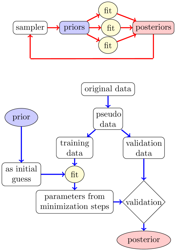
Our approach to constructing the Monte Carlo ensemble $\{\bm{a}_{k}\}$ is schematically illustrated in Fig. 1. The steps in the IMC procedure can be summarized in the following workflow:

1. Generation of the priors
   The priors are the initial parameters that are used as guess parameters for a given least-squares fit. The resulting parameters from the fits are called posteriors. During the initial iteration, a set of priors is generated using a flat sampling in the parameter space. The sampling region is selected for the shape parameters $\alpha>-1.9$ and $\beta>0$, so that the first moments of all FFs are finite. The boundary for $\beta$ restricts the distributions to be strictly zero in the $z\to 1$ limit. The upper boundaries for $\alpha$ and $\beta$ are selected to cover typical ranges observed in previous analysis HKNS07 ; DSS07 ; AKK08 . Note, however, that the posteriors can be distributed outside of the initial sampling region, if this is preferred by the data.

   For each subsequent iteration, the priors are generated from a multivariate Gaussian sampling using the covariance matrix and the central parameters from the priors of the previous iteration. The central parameters are chosen to be the median of the priors, which is found to give better convergence compared with using the mean. This sampling procedure further develops the JAM15 methodology JAM15 , where the priors were randomly selected from the previous iteration posteriors. This allows one to construct priors that are distributed more uniformly in parameter space as opposed to priors that are clustered in particular regions of parameter space. The latter can potentially bias the results if the number of priors is too small.

2. Generation of pseudodata sets
   Data resampling is performed by generating pseudodata sets using Gaussian smearing with the mean and uncertainties of the original experimental data values. Each pseudodata point $\widetilde{{\cal D}}_{i}$ is computed as

   $$\widetilde{{\cal D}}_{i}={\cal D}_{i}+R_{i}\,\alpha_{i},$$ (29)

   where for each experiment ${\cal D}_{i}$ and $\alpha_{i}$ are as in Eq. (25), and $R_{i}$ is a randomly generated number from a normal distribution of unit width. A different pseudodata set is generated for each fit in any given iteration in the IMC procedure.

3. Partition of pseudodata sets for cross-validation
   To account for possible over-fitting, the cross-validation method is incorporated. Each experimental pseudodata set is randomly divided $50\%/50\%$ into “training” and “validation” sets. However, data from any experiment with fewer than 10 points are not partitioned and are entirely included in the training set.

4. $\chi^{2}$ minimization and posterior selection
   The $\chi^{2}$ minimization procedure is performed with the training pseudodata set using the Levemberg-Marquardt lmdiff algorithm More80 . For every shift in the parameters during the minimization procedure, the $\chi^{2}$ values for both training and validation are computed and stored along with their respective parameter values, until the best fit for the training set is found. For each pseudodata set, the parameter vector that minimizes the $\chi^{2}$ of the validation is then selected as a posterior.

5. Convergence criterion
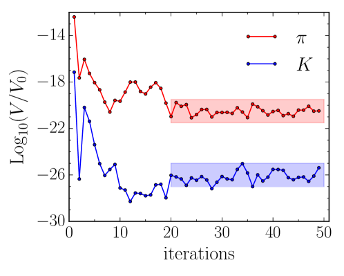
   The iterative approach of the IMC is similar to the strategy adopted in the MC VEGAS integration VEGAS . There, one constructs iteratively a grid over the parameter space such that most of the sampling is confined to regions where the integrand contributes the most, a procedure known as importance sampling. Once the grid is prepared, a large amount of samples is generated until statistical convergence of the integral is achieved.

   In Ref. JAM15 the convergence of the MC ensemble $\{\bm{a}_{k}\}$ was estimated using the $\chi^{2}$ distribution. While such an estimate can give some insight about the convergence of the posteriors, it is somewhat indirect as it does not involve the parameters explicitly. In the present analysis, we instead estimate the convergence of the eigenvalues of the covariance matrix computed from the posterior distributions. To do this we construct a measure given by

   $$V=\prod_{i}\sqrt{W_{i}},$$ (30)

   where $W_{i}$ are the eigenvalues of the covariance matrix. The quantity $V$ can be interpreted in terms of the hypervolume in the parameter space that encloses the posteriors, and is analogous to the ensemble of the most populated grid cells in a given iteration of the VEGAS algorithm VEGAS . The IMC procedure is then iterated starting from step 1, until the volume remains unchanged.

6. Generation of the Monte Carlo FF ensemble
   When the posteriors volume has reached convergence, a large number of fits is performed until the mean and expectation values of the FFs converge. The goodness-of-fit is then evaluated by calculating the overall single $\chi^{2}$ values per experiment according to

   $$\chi^{2}_{(e)}=\sum_{i}\left(\frac{\mathcal{D}_{i}^{(e)}-E[T_{i}^{(e)}]/E[N_{i}^{(e)}]}{\alpha_{i}^{(e)}}\right)^{2},$$ (31)

   which allows a direct comparison with the original unmodified data.

Finally, note that while the FF parametrization adopted here is not intrinsically more flexible than in other global analyses, the MC representation is significantly more versatile and adaptable in describing the FFs. Indeed, the resulting averaged central value of the FFs as a function of $z$ is a linear combination of many functional shapes, effectively increasing the flexibility of the parametrization.

IV Data sets

In the current analysis we use all available data sets from the single-inclusive annihilation process $e^{+}e^{-}\to hX$, for $h=\pi^{\pm}$ and $K^{\pm}$ mesons. Table 1 summarizes the various SIA experiments, including the type of observable measured (inclusive or tagged), center-of-mass energy $Q$, number of data points, and the $\chi^{2}$ values and fitted normalization factors for each data set. Specifically, we include data from experiments at DESY (from the TASSO TASSO80 ; TASSO83 ; TASSO89 and ARGUS ARGUS89 Collaborations), SLAC (TPC TPC84 ; TPC86 ; TPC88 , HRS HRS87 , SLD SLD04 and BaBar BaBar13 Collaborations), CERN (OPAL OPAL94 ; OPAL00 , ALEPH ALEPH95 and DELPHI DELPHI95 ; DELPHI98 Collaborations) and KEK (TOPAZ TOPAZ95 and Belle Belle13 ; Leitgab13 Collaborations). Approximately half of the 459 $\pi^{\pm}$ data points and 391 $K^{\pm}$ data points are near the $Z$-boson pole, $Q\approx M_{Z}$, while the most recent, high-precision Belle and BaBar data from the $B$-factories are at $Q\simeq 10.5$ GeV. The latter measurements in particular provide a more comprehensive coverage of the large-$z$ region, and reveal clearer scaling violation effects compared with the previous higher-energy measurements.

Table 1: Single-inclusive $e^{+}e^{-}$ annihilation experiments used in this analysis, inluding the type of observable (inclusive or tagged), center-of-mass energy $Q$, number of data points $N_{\rm dat}$, average fitted correlated normalization (when different from “1”), and $\chi^{2}$ values for pion and kaon production. Note that the normalization factors for the TASSO data, indicated by ^(∗) in the table, are in the range 0.976 – 1.184 for pions and 0.891 – 1.033 for kaons. For the BaBar pion data BaBar13 the “prompt” data set is used in the fit discussed in this paper, with normalization and $\chi^{2}$ values obtained using the “conventional” data set in parentheses.

experiment	ref.	observable	$Q~{}~{}~{}$	pions			kaons
			(GeV)	$~{}N_{\rm dat}$	norm.	$\chi^{2}$	$N_{\rm dat}$	norm.	$\chi^{2}$
ARGUS	ARGUS89	inclusive	9.98	35	1.024(1.058)	51.1(55.8)	15	1.007	8.5
Belle	Belle13 ; Leitgab13	inclusive	10.52	78	0.900(0.919)	37.6(21.7)	78	0.988	10.9
BaBaR	BaBar13	inclusive	10.54	39	0.993(0.948)	31.6(70.7)	30	0.992	4.9
TASSO	TASSO80 ; TASSO83 ; TASSO89	inclusive	12-44	29	$(*)$	37.0(38.8)	18	$(*)$	14.3
TPC	TPC84 ; TPC86 ; TPC88	inclusive	29.00	18	1	36.3(57.8)	16	1	47.8
		$uds$ tag	29.00	6	1	3.7( 4.6)
		$b$ tag	29.00	6	1	8.7( 8.6)
		$c$ tag	29.00	6	1	3.3( 3.0)
HRS	HRS87	inclusive	29.00	2	1	4.2( 6.2)	3	1	0.3
TOPAZ	TOPAZ95	inclusive	58.00	4	1	4.8( 6.3)	3	1	0.9
OPAL	OPAL94 ; OPAL00	inclusive	91.20	22	1	33.3(37.2)	10	1	6.3
		$u$ tag	91.20	5	1.203(1.203)	6.6( 8.1)	5	1.185	2.1
		$d$ tag	91.20	5	1.204(1.203)	6.1( 7.6)	5	1.075	0.6
		$s$ tag	91.20	5	1.126(1.200)	14.4(11.0)	5	1.173	1.5
		$c$ tag	91.20	5	1.174(1.323)	10.7( 6.1)	5	1.169	13.2
		$b$ tag	91.20	5	1.218(1.209)	34.2(36.6)	4	1.177	10.9
ALEPH	ALEPH95	inclusive	91.20	22	0.987(0.989)	15.6(20.4)	18	1.008	6.1
DELPHI	DELPHI95 ; DELPHI98	inclusive	91.20	17	1	21.0(20.2)	27	1	3.9
		$uds$ tag	91.20	17	1	13.3(13.4)	17	1	22.5
		$b$ tag	91.20	17	1	41.9(42.9)	17	1	9.1
SLD	SLD04	inclusive	91.28	29	1.002(1.004)	27.3(36.3)	29	0.994	14.3
		$uds$ tag	91.28	29	1.003(1.004)	51.7(55.6)	29	0.994	42.6
		$c$ tag	91.28	29	0.998(1.001)	30.2(40.4)	29	1.000	31.7
		$b$ tag	91.28	29	1.005(1.005)	74.6(61.9)	28	0.992	134.1
TOTAL:				459		599.3(671.2)	391		395.0
				$\chi^{2}/N_{\rm dat}=$1.31(1.46)			$\chi^{2}/N_{\rm dat}=$1.01

In the TPC, OPAL, DELPHI and SLD experiments, light-quark and heavy-quark events were separated by considering the properties of final-state hadrons. In the SLD experiment, for example, events from the primary $c$ and $b$ quarks were selected by tracks near the primary interaction point. For each secondary vertex, the total transverse momentum and invariant mass were obtained, after which the data were separated into $c$- and $b$-tagged events depending on the masses and transverse momenta. Some events without the secondary vertex were considered as light-quark ($u,d,s$)-tagged if a track did not exist with an impact parameter exceeding a certain cutoff value. Other tagged data sets used different techniques for selecting the quark-tagged events. In the OPAL experiment, separated probabilities for $u$, $d$ and $s$ quark fragmentation were also provided, which in practice provide valuable constraints on the flavor dependence in the light-quark FFs.

For the Belle measurements Belle13 , the data are provided in the form $d\sigma^{h}/dz$, and care must be taken when converting this to the hadronic FF in Eq. (1). The fragmentation energy scale $Q/2$ is reduced by initial-state (ISR) or final-state (FSR) photon radiation effects, so that the measured yield involves a variation of this scale. In practice, the energy scales in the measured events are kept within 0.5% of the nominal $Q/2$ value, and an MC simulation is performed to estimate the fraction of events with ISR or FSR photon energies $<0.5\%\times Q/2$. For each bin the measured yields are reduced by these fractions to exclude events with large ISR or FSR contributions. To convert the $d\sigma^{h}/dz$ data with the ISR/FSR cut to the total hadronic FF in Eq. (1) one therefore needs to correct the theoretical total cross section $\sigma_{\rm tot}$ by multiplying it by the ISR/FSR correction factor, which is estimated to be 0.64616(3) Belle13 ; Leitgab13 .

For the BaBar experiment BaBar13 , two data sets were provided, for “prompt” events, which contain primary hadrons or decay products of lifetimes shorter than $10^{-11}$ s, and “conventional” events, which include decays of lifetimes $(1-3)\times 10^{-11}$ s. For pions the conventional cross sections are $\sim 5\%-15\%$ larger than the prompt cross sections, while for kaons these are almost indistinguishable. The prompt data are numerically close to the LEP and SLD measurements after taking into account $Q^{2}$ evolution, although the conventional ones are technically closer to most previous measurements which included all decays. In our analysis, we consider both data sets, and assess their impact on the fits phenomenologically.

Finally, our theoretical formalism is based on the fixed-order perturbation theory, and does not account for resummations of soft-gluon logarithms or effects beyond the collinear factorization which may be important at small values of $z$. To avoid inconsistencies between the theoretical formalism and the data, cuts are applied to exclude the small-$z$ region from the analysis. In practice, we use a cut $z>0.1$ for data at energies below the $Z$-boson mass and $z>0.05$ for the data at $Q\approx M_{Z}$. For kaon data, below $z\approx 0.2$ hadron mass corrections are believed to play a more prominent role AAR15 . Since these are not considered in this analysis, we apply the cut $z>0.2$ for the low-$Q$ kaon data sets from ARGUS and BaBar.

V Analysis results

In this section we present the main results of our IMC analysis. We first establish the stability of the IMC procedure by examining specific convergence criteria, and then illustrate the results for the fragmentation functions through comparisons with data and previous analyses. Programs for generating the FFs obtained in this analysis, which we dub “JAM16FF”, can be downloaded from Ref. JAMgit .

V.1 IMC convergence

We examine two types of convergence tests of the IMC procedure, namely, the iterative convergence of the priors (the “grid”), and the convergence of the final posterior distributions. As discussed in Section III.2, the convergence of the priors can be tested by observing the variation of the volume $V$ with the number of iterations, as shown in Fig. 2. For each iteration 200 fits are performed. During the initial $\sim 10$ iterations, the volume changes some 9 orders of magnitude, indicating a very rapid variation of the prior distribution. After $\sim 30$ iterations, the volume becomes relatively stable, with statistical fluctuations around 2 orders magnitude due to finite statistics. The stability of the prior volume indicates that the region of interest in the parameter space has been isolated by the IMC procedure.

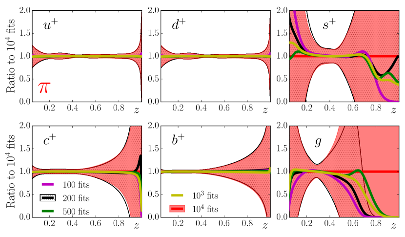
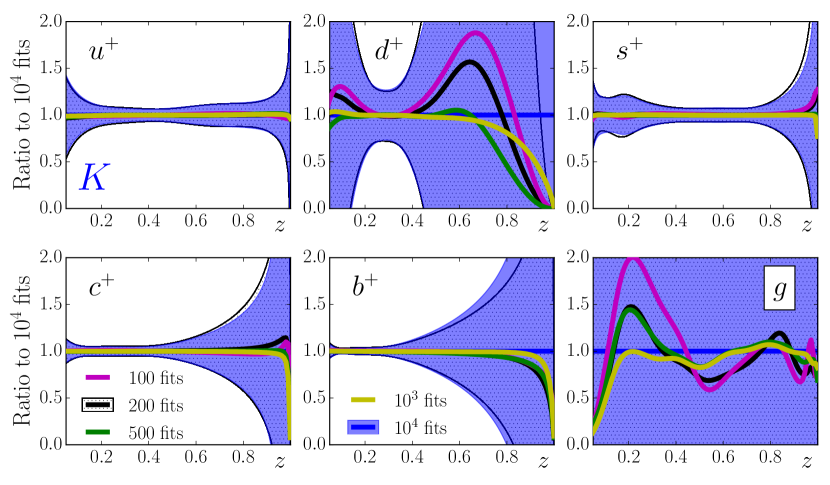
Having obtained an optimal MC priors sample, a final iteration is performed with $10^{4}$ fits. In Fig. 3 we illustrate the statistical properties of the final posterior distribution by showing averaged ratios of FFs with smaller samples (100, 200, 500 and 1000) relative to the total $10^{4}$ samples (the averaged error bands are displayed only for the 200 and $10^{4}$ samples). Using 200 posterior samples, one obtains uncertainty bands that are comparable with those with $10^{4}$ samples. For the central values most of the FFs with 200 samples agree well with the $10^{4}$ samples. Some exceptions are the $D^{\pi}_{s^{+}}$, $D^{\pi}_{g}$, $D^{K}_{d^{+}}$ and $D^{K}_{g}$ FFs; however, here the differences are in regions where the FFs are poorly determined and the relative error bands are large. For practical applications these effects will be irrelevant, and using a sample of 200 posteriors will be sufficient to give an accurate representation of FFs. Unless otherwise stated the results presented in the following use 200 fits from the final sample.

V.2 SIA cross sections

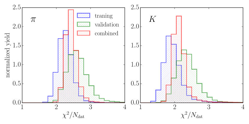
In Fig. 4 the normalized yields of the final posteriors versus $\chi^{2}$ per datum for the training and validation sets are presented using the full sample of $10^{4}$ fits. In the ideal Gaussian limit, the distributions are expected to peak around 2 JAM15 . In practice, inconsistencies between data sets shift the peak of the distribution to larger $\chi^{2}/N_{\rm dat}$ values. This is evident for the pion production case in Fig. 4, where the $\chi^{2}/N_{\rm dat}$ distribution peaks around 2.5. In contrast, for kaon production the distribution peaks around 2.1. We stress, however, that even if the peak occurs at 2, it does not imply consistency among the data sets (or data vs. theory), since the larger experimental uncertainties in the kaon data sets compared with the pion can induce such behavior.

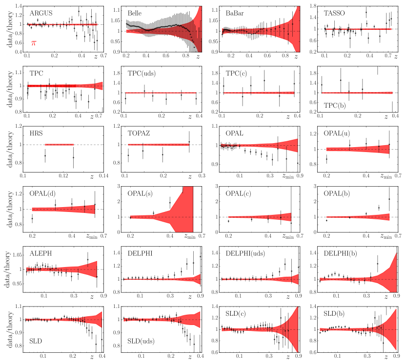
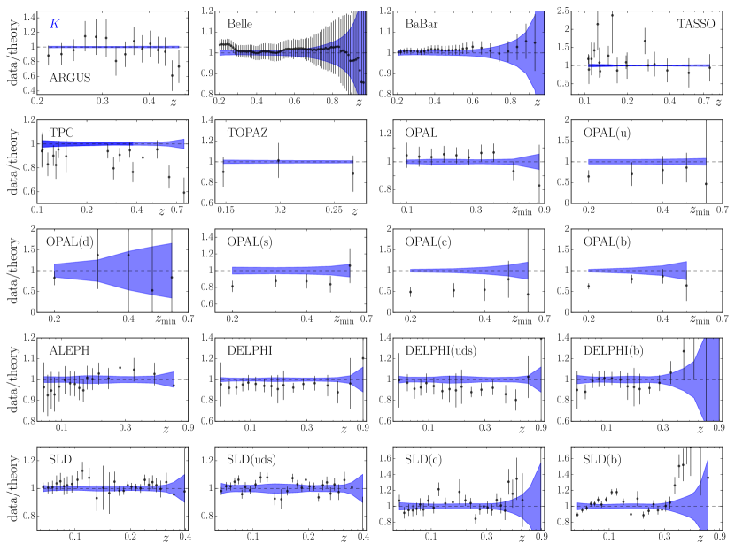
The ratios of experimental SIA cross sections to the fitted values are shown in Figs. 5 and 6 for pions and kaons, respectively. For the pion production data, at the lower energies $Q\lesssim 30$ GeV there is good overall agreement between the fitted cross sections and the data, with the exception of a few sets (TPC, HRS and TOPAZ) that differ by $\sim 5-10\%$, within relatively large errors. Interestingly, the older ARGUS data ARGUS89 are consistent with the recent high-precision measurements from Belle Belle13 ; Leitgab13 and BaBar BaBar13 . We find, however, that the Belle pion data require an $\approx 10\%$ normalization, which may be related to the overall normalization correction from initial state radiation effects Leitgab13 or other corrections. This should not, however, affect the $z$ dependence of the extracted FFs.

A relatively good description is also obtained of the data at higher energies, $Q=M_{Z}$, which generally have smaller uncertainties, although some discrepancies appear at higher $z$ values. In particular, an inconsistency is apparent between the shapes of the DELPHI DELPHI95 ; DELPHI98 and SLD SLD04 spectra at $z\gtrsim 0.4$ for both inclusive and $uds$-tagged data, with the DELPHI data lying systematically above the fitted results and SLD data lying below. For the heavy quark tagged results the agreement with DELPHI and SLD data is generally better, with only some deviations at the highest $z$ values where the errors are largest. The OPAL tagged data OPAL94 ; OPAL00 are the only ones that separate the individual light quark flavors $u$, $d$ and $s$ from the heavy flavors. The latter have rather large $\chi^{2}$ values for both pion and kaon data sets, particularly the $b$–tagged sample of the pion case. While the unfavored $d$–tagged kaon sample is well described in the fit, the unfavored $s$–tagged pion data appear less consistent with the theory. In all cases the OPAL tagged data require a normalization of $\approx 20\%$. Note that the observable for the OPAL data is the $z$-integrated cross section from $z_{\rm min}$ to 1.

The total $\chi^{2}/N_{\rm dat}$ for the resulting fit to all pion data sets is $\approx 1.31$. Using the conventional BaBar pion data set instead of the prompt gives a slightly worse overall fit, with $\chi^{2}/N_{\rm dat}=1.46$, with the difference coming mostly from the BaBar and TPC inclusive data sets. The Belle data, on the other hand, are better fitted when the conventional BaBar data set is used. Since the conventional BaBar data lie $\sim 10\%$ higher than the prompt, which themselves lie slightly below the Belle data, the Belle cross sections require a normalization shift that is closer to that needed for the conventional BaBar data.

For the kaon cross sections, the overall agreement between theory and experiment is slightly better than for pions, mostly because of the relatively larger uncertainties on the $K$ data. At low energies, as was the case for pions, the TPC data TPC84 ; TPC86 ; TPC88 lie $\approx 10\%$ below the global fit. Interestingly, though, the Belle kaon data Belle13 ; Leitgab13 do not require as large a normalization shift as was needed for the Belle pion data in Fig. 5. At energies near the $Z$-boson pole, $Q=M_{Z}$, the deviations at large $z$ between the theoretical and experimental cross sections are not as prominent as for pions, with only the SLD heavy quark tagged data SLD04 exhibiting any significant disagreement. The OPAL flavor-tagged data OPAL94 ; OPAL00 generally prefer an $\approx 10-15\%$ normalization for all quark flavors. The DELPHI inclusive and light quark tagged data DELPHI95 ; DELPHI98 , which do not include an overall normalization parameter, appear to systematically lie $\approx 10\%$ below the fitted results across most of the $z$ range. Fits to other high energy data sets generally give good agreement, and the $\chi^{2}/N_{\rm dat}$ value for the combined kaon fit is found to be $1.01$.

V.3 Fragmentation functions

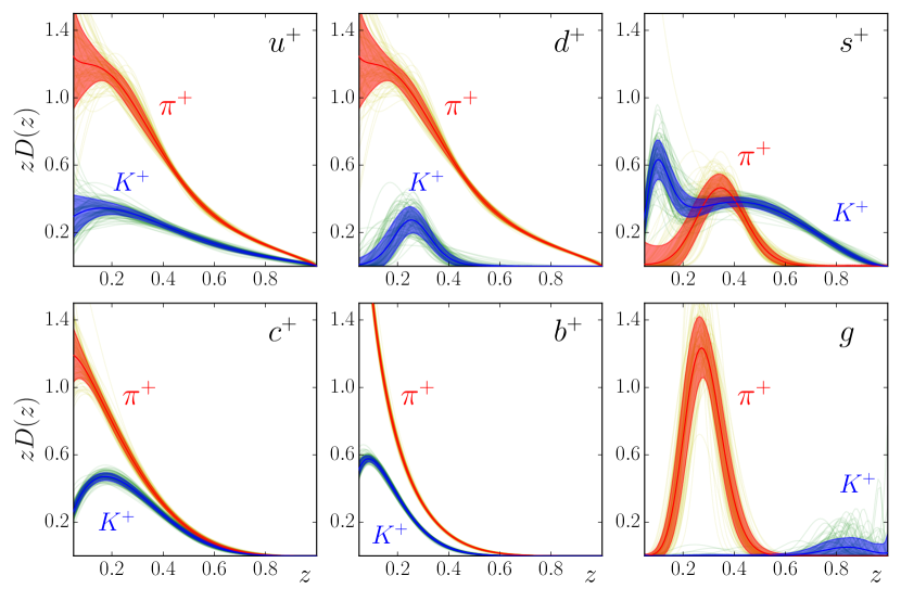
The fragmentation functions resulting from our IMC analysis are shown in Fig. 7 at the input scale, which is taken to be $Q^{2}=1$ GeV² for the $u$, $d$, $s$ and $g$ flavors and at the mass thresholds $Q^{2}=m_{q}^{2}$ for the heavy $c$ and $b$ quarks. The curve bundles represent random samples of 100 posteriors from the full set of fitted results, with the central values and variance bands computed from Eqs. (21) and (22) using the 200 posteriors selected for the final JAM16FF results JAMgit . Generally the pion FFs have a larger magnitude than the kaon FFs, with the exception of the strange quark, where the $s^{+}$ to kaon distribution $D_{s^{+}}^{K^{+}}$ is larger than that for the pion, $D_{s^{+}}^{\pi^{+}}$, over most of the $z$ range. As expected, the $u^{+}$ and $d^{+}$ FFs to $\pi^{+}$, which correspond to sums of favored and unfavored distributions and reflect the valence structure of the pion, are dominant at intermediate and large values of $z$, $z\gtrsim 0.2$. In the limit of exact isospin symmetry (neglecting mass differences between $u$ and $d$ quarks), these are in fact identical, $D_{u^{+}}^{\pi^{+}}=D_{d^{+}}^{\pi^{+}}$. The $s^{+}$ to pion distribution, in contrast, is smaller in magnitude, with a peak value at $x\sim 0.3-0.4$ that is less than $\approx 1/2$ that for the nonstrange quarks. Since this distribution is entirely unfavored, and constrained mostly by the scant flavor-tagged data, it has somewhat larger uncertainties compared with the nonstrange FFs. Note that our analysis uses two shapes for the favored $D_{u^{+}}^{\pi^{+}}=D_{d^{+}}^{\pi^{+}}$ FFs, but one shape for all other pion distributions, Eqs. (19).

For the heavy quark FFs to pions, the characteristic differences between the $s^{+}$, $c^{+}$ and $b^{+}$ distributions generally reflect the different masses of the quarks, with larger mass corresponding to softer distributions. The $c^{+}$ and $b^{+}$ FFs, in particular, are large at low $z$ values, $z\lesssim 0.1$, and comparable to the light-quark FFs evolved to the same scale. (Note that the heavy quark distributions exist only above the mass threshold, $Q>m_{q}$.) The gluon FF $D_{g}^{\pi^{+}}$ is less singular, but is strongly peaked at $z\approx 0.25$ at the input scale. Its uncertainties are also larger than those for the favored distributions, as their effects on the SIA cross sections are of higher order in $\alpha_{s}$.

For the fragmentation to kaons, one of the most conspicuous differences with pions is the large magnitude of the strange FF $D_{s^{+}}^{K^{+}}$ at intermediate and high values of $z$, where it is comparable to the $u^{+}$ and $d^{+}$ FFs to pions. Reflecting the valence quark structure of $K^{\pm}$, the $D_{u^{+}}^{K^{+}}$ FF is also similar in size, but because of the mass difference between the strange and nonstrange light quarks there is no reason for the favored $u^{+}$ and $s^{+}$ fragmentation to kaons to be equal. In fact, we find $D_{s^{+}}^{K^{+}}\gtrsim D_{u^{+}}^{K^{+}}$ at high values of $z$. Unlike for pions, the $d^{+}$ fragmentation to kaons is unfavored, $D_{d^{+}}^{K^{+}}\ll D_{u^{+}}^{K^{+}}$, with relatively large uncertainties, peaking at $z\sim 0.1$ and playing a role similar to that of $s^{+}$ fragmentation to $\pi^{+}$. The heavy quark FFs to kaons are also sizeable compared with the light quark functions, but peak at slightly larger $z$ values than the corresponding pion FFs. The gluon FF to kaons, $D_{g}^{K^{+}}$, peaks at rather high $z$ values, $z\approx 0.85$, at the input scale, consistent with the findings of some earlier analyses HKNS07 , and is very small in magnitude.

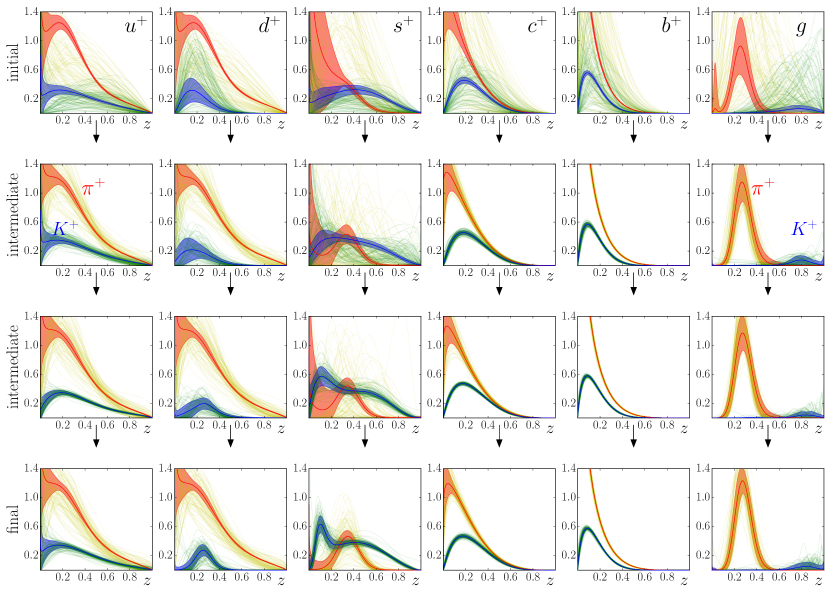
The unusual shapes of some of the FFs, such as the gluon to $\pi^{+}$ and $K^{+}$ or the unfavored light quark FFs, lead to the natural question of whether these are robust distributions or possibly artifacts of the fitting procedure. We can address this by observing snapshots in the IMC chain, as illustrated in Fig. 8, where the FFs from selected iteration steps are plotted at the input scale as a function of $z$. The first and last rows in Fig. 8 show the initial and final steps in the IMC procedure, respectively. In addition to the posterior shapes and uncertainties, we display in each row the prior distributions as individual curves. After performing the initial iteration, the large spread in the prior FFs due to the flat sampling of the parameter space is reduced significantly, especially for distributions that are more strongly constrained by the SIA data. For the FFs that are less directly constrained by the data, more iterations are needed before convergence is reached, as illustrated by the $s^{+}$ to $\pi^{+}$ distribution, for example. We find that after $\approx 30$ iterations all of the distributions become stable, which is consistent with the convergence of the volumes observed in Fig. 2.

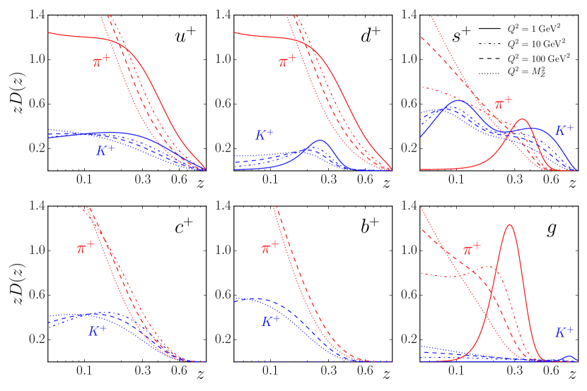
Although the peaks in some of the FFs, such as $D_{g}^{\pi^{+},K^{+}}$ and $D_{s^{+}}^{\pi^{+}}$, are prominent at the input scale, after $Q^{2}$ evolution these become largely washed out. This is illustrated in Fig. 9, where the FFs are evolved to a common scale for all FFs that are above the quark threshold, namely at $Q^{2}=1,10$ and 100 GeV² and at the $Z$-boson pole, $Q^{2}=M_{Z}^{2}$. Recall that the lowest $Q^{2}$ in any of the data sets is $\approx 100$ GeV², so the shapes at $Q^{2}=1$ and 10 GeV² are not directly compared with experimental data and are shown for illustration only.

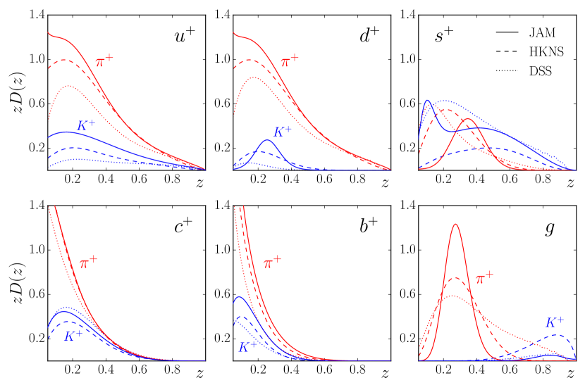
Compared with parametrizations from other global FF analyses, our fitted FFs are qualitatively similar for the most part, but reveal important differences for specific distributions, as Fig. 10 illustrates. For pions, our $u^{+}$ and $d^{+}$ distributions are close to the HKNS HKNS07 and DSS DSS07 results at large $z$, but are $\sim 20\%-30\%$ larger in magnitude at low $z$ values, $z\lesssim 0.3$. The strange quark to pion FF peaks at somewhat larger $z$ than the nonstrange, with a magnitude similar to that in previous fits. The peak in the gluon FF at $z\approx 0.25$ coincides with that in the HKNS and DSS gluon FFs, but our distribution is rather more narrow with a smaller large-$z$ tail.

The comparison between the various parametrizations for the kaon FFs is quite instructive, especially for the light quark flavors and the gluon. The favored $D_{u^{+}}^{K^{+}}$ and $D_{s^{+}}^{K^{+}}$ FFs in our fit turn out to be of comparable magnitude, with the $u^{+}$ closer to the HKNS results and $s^{+}$ closer to DSS. In particular, for the $u$ quark to kaon FF our result is $\approx 30\%-50\%$ larger than HKNS, but some 2–3 times greater than DSS over the range $0.2\lesssim z\lesssim 0.9$. On the other hand, the strange to kaon FF lies between the HKNS and DSS results at intermediate $z$ values, but coincides with the DSS at $z\gtrsim 0.5$. Interestingly, we do not observe the large excess of $s$ to $K$ fragmentation over $u$ to $K$ found in the DSS analysis, which has important phenomenological consequences for the extraction of the polarized strange quark PDF from semi-inclusive DIS data LSS11 ; LSS15 .

Recall that in our analysis we use two shapes for the favored $D_{u^{+}}^{K^{+}}$ and $D_{s^{+}}^{K^{+}}$ FFs, Eqs. (20), and one shape for all other kaon distributions. In contrast, previous analyses HKNS07 ; DSS07 parametrized the $u^{+}$ and (the unfavored) $\bar{u}$ functions separately, assuming that at the input scale $D_{\bar{u}}^{K^{+}}=D_{d}^{K^{+}}=D_{\bar{d}}^{K^{+}}$. In contrast, with the IMC procedure in the present analysis we do not impose any relation between the $\bar{u}$ and $\bar{d}$ FFs, parametrizing only the $q^{+}$ distributions as constrained by data.

For the gluon to kaon FF we find a similarly hard distribution as in earlier analyses, peaking at rather large $z$ values, $z\sim 0.8$ at the input scale. The harder shape of $D_{g}^{K^{+}}$ compared with $D_{g}^{\pi^{+}}$ can be understood in terms of the higher energy needed for a gluon to split to an $s\bar{s}$ pair than to a $u\bar{u}$ or $d\bar{d}$ pair in the pion case HKNS07 .

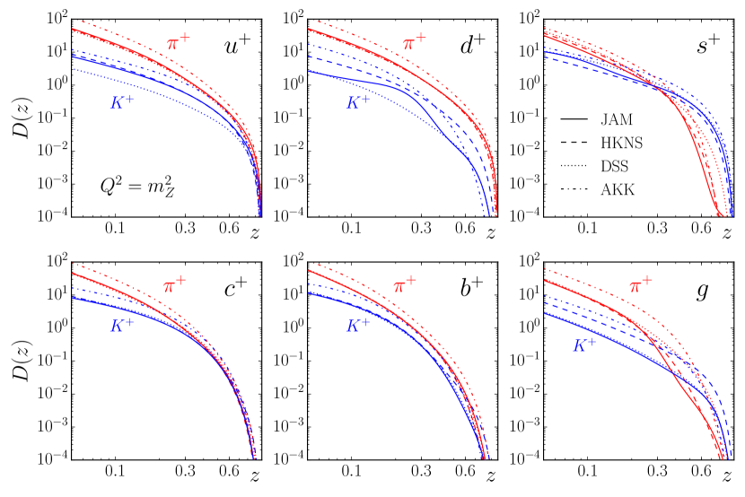
Despite the striking shape of the gluon FF at the input scale, it is almost entirely washed out after $Q^{2}$ evolution to the $Z$-boson scale, as Fig. 11 illustrates. Here the FFs $D(z)$ (rather than $zD(z)$) are compared for the HKNS HKNS07 , DSS DSS07 and the AKK AKK08 parametrizations. Viewed on a logarithmic scale, the qualitative features of the shapes of FFs are similar across all the parametrizations, especially the HKNS, DSS and the present fit. The AKK results generally lie above the other parametrizations in the low-$z$ region, while more variation is observed at higher $z$ values.

VI Conclusion

We have performed the first Monte Carlo based QCD analysis for parton to hadron fragmentation functions within collinear factorization, using all existing single-inlusive $e^{+}e^{-}$ annihilation data into pions and kaons. In particular, we include the recent high-precision SIA data from the Belle Belle13 ; Leitgab13 and BaBar BaBar13 Collaborations, which significantly extend the kinematical coverage to large values of $z$.

Our analysis is based on the iterative Monte Carlo approach, first adopted in the recent QCD analysis of polarized PDFs JAM15 , which provides a robust determination of expectation values and uncertainties for the FFs. We further extended this methodology by sampling new priors from previous iterations using a multivariate Gaussian distribution, implementing a new strategy for assessing the convergence of the IMC chain by considering the covariance matrix of the posterior distributions. This allowed us to sample fairly the parameter eigenspace after each iteration instead of the posteriors, which can exhibit several distinct solutions. We find that an accurate representation of the FFs can be attained with a sample of 200 fits.

We obtained a relatively good overall description of the pion and kaon SIA data at both low and high center-of-mass energies, despite some tensions between the high-energy DELPHI and SLD pion data sets in the large-$z$ region. For the kaon data a very good $\chi^{2}/N_{\rm dat}\sim 1$ was achieved, partly because of larger experimental uncertainties and also less evident tensions between data sets.

The shapes of the pion FFs are qualitatively similar to those found in previous analyses, with the exception of the unfavored $D_{s^{+}}^{\pi^{+}}$ and the $D_{g}^{\pi^{+}}$ distributions. The latter is more strongly peaked around the maximum at small $z$ values than either the HKNS or DSS results, while the former has a somewhat harder $z$ distribution. The kaon FFs, on the other hand, show greater deviation from the earlier results. Here, the favored $D_{s^{+}}^{K^{+}}$ function is similar in magnitude to that from the DSS parametrization DSS07 for $0.5\lesssim z\lesssim 1$, but displays important differences at $z\lesssim 0.5$ that stem from the greater flexibility of the parametrization used in our analysis. We also find a larger magnitude of the $D_{u^{+}}^{K^{+}}$ FF at moderate to low $z$ values compared with the DSS fit in particular. In contrast, the gluon to kaon distribution, which peaks at very large $z$ values, $z\sim 0.85$, but with a very small magnitude, is consistent with the DSS result. The disparity between the fitted $D_{g}^{\pi^{+}}$ and $D_{g}^{K^{+}}$ functions is particularly striking. At energies on the order of the $Z$-boson mass, the evolved distributions are much more similar to those of the previous analyses, with the exception of the $D_{g}^{\pi^{+}}$ and $D_{s^{+}}^{\pi^{+}}$ FFs.

The partial separation of the FFs for the various quark flavors has been possible because of the existence of the tagged flavor data and the $Q^{2}$ dependence of SIA cross sections, from low $Q\sim 10$ GeV up to the $Z$-boson mass, selecting differently weighted combinations of FFs in the $\gamma$ and $Z$-exchange cross sections. To further decompose the quark and antiquark FFs, and better constrain the gluon fragmentation, additional information will be needed from SIDIS and meson production in $pp$ collisions. More immediately, it will be particularly interesting to examine the effect of the strange to kaon fragmentation on the extraction of the polarized strange quark PDF $\Delta s$ from SIDIS data. A combined analysis of polarized DIS and SIDIS data and SIA cross sections is currently in progress SIDIS16 .

Appendix A Hard scattering coefficients

For completeness, in this appendix we give the hard coefficient functions in Mellin moment space at NLO. For the quark case, the NLO coefficient is Kretzer00 ; GRV90

$$\widetilde{{\bm{H}}}^{(1)}_{q}(N,Q^{2},\mu_{R}^{2}=Q^{2},\mu_{\rm FF}^{2}) = 2\,C_{F}\biggr{[}5S_{2}(N)+S_{1}^{2}(N)+S_{1}(N)\left(\frac{3}{2}-\frac{1}{N(N+1)}\right)-\frac{2}{N^{2}}$$ (32)

$$\hskip 28.45274pt+\frac{3}{(N+1)^{2}}-\frac{3}{2}\frac{1}{(N+1)}-\frac{9}{2}+\frac{1}{N}$$

$$\hskip 28.45274pt+\left(\frac{1}{N(N+1)}-2S_{1}(N)+\frac{3}{2}\right)\ln\frac{Q^{2}}{\mu_{\rm FF}^{2}}\biggr{]},$$

while for the gluon one has

$$\widetilde{{\bm{H}}}^{(1)}_{g}(N,Q^{2},\mu_{R}^{2}=Q^{2},\mu_{\rm FF}^{2}) = 4\,C_{F}\biggr{[}-S_{1}(N)\frac{N^{2}+N+2}{(N-1)N(N+1)}-\frac{4}{(N-1)^{2}}+\frac{4}{N^{2}}$$ (33)

$$-\frac{3}{(N+1)^{2}}+\frac{4}{(N-1)N}+\frac{N^{2}+N+2}{N(N^{2}-1)}\ln\frac{Q^{2}}{\mu_{\rm FF}^{2}}\biggr{]},$$

where $C_{F}=4/3$. Here the harmonic sums $S_{1}(N)$ and $S_{2}(N)$ can be written in terms of the Euler-Mascheroni constant $\gamma_{E}$, the polygamma function $\psi_{N}$, and the Riemann zeta function $\zeta$, analytically continued to complex values of $N$ GRV90 ,

$$S_{1}(N) = \sum_{j=1}^{N}\frac{1}{j}\ \longrightarrow\ \gamma_{E}+\psi^{(0)}_{N+1},$$ (34)

$$S_{2}(N) = \sum_{j=1}^{N}\frac{1}{j^{2}}\ \longrightarrow\ \zeta(2)-\psi^{(1)}_{N+1},$$ (35)

where the $m$-th derivative of the polygamma function $\psi^{(m)}_{N}$ is given by

$$\psi^{(m)}_{N} = \frac{d^{m}\psi_{N}}{dN^{m}}\ =\ \frac{d^{m+1}\ln\Gamma(N)}{dN^{m+1}}.$$ (36)

Appendix B Timelike splitting functions

The $N$-th moments of the splitting functions in the timelike region, up to ${\cal O}(a_{s}^{3})$ corrections, can be written for the general case when $\mu_{\rm R}\neq\mu_{\rm FF}$ as PEGASUS

$${\bm{P}}_{ij}(N,\mu_{\rm R}^{2},\mu_{\rm FF}^{2}) = a_{s}(\mu_{\rm R}^{2})\,{\bm{P}}_{ij}^{(0)}(N)\,+\,a_{s}^{2}(\mu_{\rm R}^{2})\,\Big{(}{\bm{P}}_{ij}^{(1)}(N)-\beta_{0}{\bm{P}}_{\rm NS}^{(0)}(N)\ln\frac{\mu_{\rm FF}^{2}}{\mu_{\rm R}^{2}}\Big{)},$$ (37)

where $\beta_{0}=11-2n_{f}/3$. At leading order the timelike splitting function moments are given by the well-known expressions Floratos81 ; Weigl96

$${\bm{P}}^{(0)}_{\rm NS^{\pm}} = {\bm{P}}^{(0)}_{qq}\ =\ -C_{F}\left[4S_{1}(N)-3-\frac{2}{N(N+1)}\right],$$ (38a)

$${\bm{P}}^{(0)}_{qg} = 4n_{f}C_{F}\frac{N^{2}+N+2}{N(N-1)(N+1)},$$ (38b)

$${\bm{P}}^{(0)}_{gq} = \frac{N^{2}+N+2}{N(N+1)(N+2)},$$ (38c)

$${\bm{P}}^{(0)}_{gg} = -C_{A}\left[4S_{1}(N)-\frac{11}{3}-\frac{4}{N(N-1)}-\frac{4}{(N+1)(N+2)}\right]-\frac{2n_{f}}{3},$$ (38d)

where $C_{A}=3$. Note that our notation for the off-diagonal timelike splitting functions ${\bm{P}}^{(0)}_{qg}$ and ${\bm{P}}^{(0)}_{gq}$ is opposite to that in Ref. GRV93 .

At NLO accuracy, the timelike splitting function moments are given by Floratos81 ; GRV93 ; Curci80

$${\bm{P}}^{(1)}_{\rm NS^{\pm}} = -C^{2}_{F}\left[8S_{1}(N)\frac{(2N+1)}{N^{2}(N+1)^{2}}+8\left(2S_{1}(N)-\frac{1}{N(N+1)}\right)\big{(}S_{2}(N)-S_{2\pm}^{\prime}(\tfrac{N}{2})\big{)}\right.$$ (39a)

$$\left.+12S_{2}(N)+32\widetilde{S}_{\pm}(N)-4S_{3\pm}^{\prime}(\tfrac{N}{2})-\frac{3}{2}-4\frac{(3N^{3}+N^{2}-1)}{N^{3}(N+1)^{3}}\mp 8\frac{(2N^{2}+2N+1)}{N^{3}(N+1)^{3}}\right]$$

$$- C_{A}C_{F}\left[\frac{268}{9}S_{1}(N)-4\left(2S_{1}(N)-\frac{1}{N(N+1)}\right)\big{(}2S_{2}(N)-S_{2\pm}^{\prime}(\tfrac{N}{2})\big{)}-\frac{44}{3}S_{2}(N)-\frac{17}{6}\right.$$

$$\left.-16\widetilde{S}_{\pm}(N)+2S_{3\pm}^{\prime}(\tfrac{N}{2})-\frac{2}{9}\frac{(151N^{4}+236N^{3}+88N^{2}+3N+18)}{N^{3}(N+1)^{3}}\pm 4\frac{(2N^{2}+2N+1)}{N^{3}(N+1)^{3}}\right]$$

$$- \frac{1}{2}n_{f}C_{F}\left[-\frac{80}{9}S_{1}(N)+\frac{16}{3}S_{2}(N)+\frac{2}{3}+\frac{8}{9}\frac{(11N^{2}+5N-3)}{(N^{2}(N+1)^{2})}\right]\ +\ \Delta_{\rm NS}^{(1)},$$

$${\bm{P}}^{(1)}_{qq} = {\bm{P}}^{(1)}_{\rm NS^{+}}\ +\ n_{f}C_{F}\left[\frac{(5N^{5}+32N^{4}+49N^{3}+38N^{2}+28N+8)}{(N-1)N^{3}(N+1)^{3}(N+2)^{2}}\right]+\ \Delta_{qq}^{(1)},$$ (39b)

$${\bm{P}}^{(1)}_{gg} = -\frac{1}{2}n_{f}C_{A}\left[-\frac{80}{9}S_{1}(N)+\frac{16}{3}+\frac{8}{9}\frac{(38N^{4}+76N^{3}+94N^{2}+56N+12)}{(N-1)N^{2}(N+1)^{2}(N+2)}\right]$$ (39c)

$$- \frac{1}{2}n_{f}C_{F}\left[4+8\frac{(2N^{6}+4N^{5}+N^{4}-10N^{3}-5N^{2}-4N-4)}{(N-1)N^{3}(N+1)^{3}(N+2)}\right]$$

$$- C^{2}_{A}\left[\frac{268}{9}S_{1}(N)+32S_{1}(N)\frac{(2N^{5}+5N^{4}+8N^{3}+7N^{2}-2N-2)}{(N-1)^{2}N^{2}(N+1)^{2}(N+2)^{2}}-\frac{32}{3}\right.$$

$$\hskip 19.91684pt+16S_{2+}^{\prime}(\tfrac{N}{2})\frac{(N^{2}+N+1)}{(N-1)N(N+1)(N+2)}-8S_{1}(N)S_{2+}^{\prime}(\tfrac{N}{2})+16\widetilde{S}_{+}(N)-2S_{3+}^{\prime}(\tfrac{N}{2})$$

$$\hskip 19.91684pt-\frac{2}{9}\frac{(457N^{9}+2742N^{8}+6040N^{7}+6098N^{6}+1567N^{5}-2344N^{4}-1632N^{3})}{(N-1)^{2}N^{3}(N+1)^{3}(N+2)^{3}}$$

$$\left.\hskip 19.91684pt-\frac{2}{9}\frac{(560N^{2}+1488N+576)}{(N-1)^{2}N^{3}(N+1)^{3}(N+2)^{3}}\right]+\ \Delta_{gg}^{(1)},$$

$${\bm{P}}^{(1)}_{qg} = 2n_{f}C_{F}^{2}\left[\left(S_{1}^{2}(N)-3S_{2}(N)-\frac{2\pi^{2}}{3}\right)\frac{(N^{2}+N+2)}{(N-1)N(N+1)}\right.$$

$$\hskip 19.91684pt+2S_{1}(N)\left(\frac{4}{(N-1)^{2}}-\frac{2}{(N-1)N}-\frac{4}{N^{2}}+\frac{3}{(N+1)^{2}}-\frac{1}{(N+1)}\right)-\frac{8}{(N-1)^{2}N}$$

$$\left.\hskip 19.91684pt+\frac{8}{(N-1)N^{2}}+\frac{2}{N^{3}}+\frac{8}{N^{2}}-\frac{1}{2N}+\frac{1}{(N+1)^{3}}-\frac{5}{2(N+1)^{2}}+\frac{9}{2(N+1)}\right]$$

$$+ 2n_{f}C_{F}C_{A}\left[\left(-S_{1}^{2}(N)+5S_{2}(N)-G^{(1)}(N)+\frac{\pi^{2}}{6}\right)\frac{(N^{2}+N+2)}{(N-1)N(N+1)}\right.$$

$$\hskip 19.91684pt+2S_{1}(N)\left(-\frac{2}{(N-1)^{2}}+\frac{2}{(N-1)N}+\frac{2}{N^{2}}-\frac{2}{(N+1)^{2}}+\frac{1}{N+1}\right)$$

$$\hskip 19.91684pt-\frac{8}{(N-1)^{3}}+\frac{6}{(N-1)^{2}}+\frac{17}{9(N-1)}+\frac{4}{(N-1)^{2}N}-\frac{12}{(N-1)N^{2}}-\frac{8}{N^{2}}+\frac{5}{N}$$

$$\left.\hskip 19.91684pt-\frac{2}{N^{2}(N+1)}-\frac{2}{(N+1)^{3}}-\frac{7}{(N+1)^{2}}-\frac{1}{N+1}-\frac{8}{3(N+2)^{2}}+\frac{44}{9(N+2)}\right],$$

$${\bm{P}}^{(1)}_{gq} = \frac{1}{3}n_{f}\left[S_{1}(N+1)\frac{(N^{2}+N+2)}{N(N+1)(N+2)}+\frac{1}{N^{2}}-\frac{5}{3N}-\frac{1}{N(N+1)}-\frac{2}{(N+1)^{2}}\right.$$ (39e)

$$\left.\hskip 19.91684pt+\frac{4}{3(N+1)}+\frac{4}{(N+2)^{2}}-\frac{4}{3(N+2)}\right]$$

$$+ \frac{1}{4}C_{F}\left[\Big{(}-2S_{1}^{2}(N+1)+2S_{1}(N+1)+10S_{2}(N+1)\Big{)}\frac{(N^{2}+N+2)}{N(N+1)(N+2)}\right.$$

$$\hskip 19.91684pt+4S_{1}(N+1)\left(-\frac{1}{N^{2}}+\frac{1}{N}+\frac{1}{N(N+1)}+\frac{2}{(N+1)^{2}}-\frac{4}{(N+2)^{2}}\right)$$

$$\hskip 19.91684pt-\frac{2}{N^{3}}+\frac{5}{N^{2}}-\frac{12}{N}+\frac{4}{N^{2}(N+1)}-\frac{12}{N(N+1)^{2}}-\frac{6}{N(N+1)}$$

$$\left.\hskip 19.91684pt+\frac{4}{(N+1)^{3}}-\frac{4}{(N+1)^{2}}+\frac{23}{N+1}-\frac{20}{N+2}\right]$$

$$+ \frac{1}{4}C_{A}\left[\left(2S_{1}^{2}(N+1)-\frac{10}{3}S_{1}(N+1)-6S_{2}(N+1)+2G^{(1)}(N+1)-\pi^{2}\right)\right.$$

$$\hskip 42.67912pt\times\frac{(N^{2}+N+2)}{N(N+1)(N+2)}$$

$$\hskip 19.91684pt-4S_{1}(N+1)\left(-\frac{2}{N^{2}}+\frac{1}{N}+\frac{1}{N(N+1)}+\frac{4}{(N+1)^{2}}-\frac{6}{(N+2)^{2}}\right)$$

$$\hskip 19.91684pt-\frac{40}{9(N-1)}+\frac{4}{N^{3}}+\frac{8}{3N^{2}}+\frac{26}{9N}-\frac{8}{N^{2}(N+1)^{2}}+\frac{22}{3N(N+1)}+\frac{16}{(N+1)^{3}}$$

$$\left.\hskip 19.91684pt+\frac{68}{3(N+1)^{2}}-\frac{190}{9(N+1)}+\frac{8}{(N+1)^{2}(N+2)}-\frac{4}{(N+2)^{2}}+\frac{356}{9(N+2)}\right],$$

where the terms

$$\Delta_{\rm NS}^{(1)} = C_{F}^{2}\left[-4S_{1}(N)+3+\frac{2}{N(N+1)}\right]\left[2S_{2}(N)-\frac{\pi^{2}}{3}-\frac{2N+1}{N^{2}(N+1)^{2}}\right],$$ (40a)

$$\Delta_{qq}^{(1)} = \frac{1}{2}n_{f}C_{F}\left[-\frac{80}{9}\frac{1}{N-1}+\frac{8}{N^{3}}+\frac{12}{N^{2}}-\frac{12}{N}+\frac{8}{(N+1)^{3}}+\frac{28}{(N+1)^{2}}\right.$$ (40b)

$$\left.\hskip 17.07182pt-\ \frac{4}{N+1}+\frac{32}{3}\frac{1}{(N+2)^{2}}+\frac{224}{9}\frac{1}{N+2}\right],$$

$$\Delta_{gg}^{(1)} = \frac{1}{2}n_{f}C_{F}\left[-\frac{16}{3}\frac{1}{(N-1)^{2}}+\frac{80}{9}\frac{1}{N-1}+\frac{8}{N^{3}}-\frac{16}{N^{2}}+\frac{12}{N}+\frac{8}{(N+1)^{3}}\right.$$ (40c)

$$\left.\hskip 36.98866pt-\ \frac{24}{(N+1)^{2}}+\frac{4}{N+1}-\frac{16}{3}\frac{1}{(N+2)^{2}}-\frac{224}{9}\frac{1}{N+2}\right]$$

$$- \frac{4}{3}n_{f}C_{A}\left[S_{2}(N)-\frac{1}{(N-1)^{2}}+\frac{1}{N^{2}}-\frac{1}{(N+1)^{2}}+\frac{1}{(N+2)^{2}}-\frac{\pi^{2}}{6}\right]$$

$$+ C_{A}^{2}\left[-8S_{1}(N)S_{2}(N)+8S_{1}(N)\left(\frac{1}{(N-1)^{2}}-\frac{1}{N^{2}}+\frac{1}{(N+1)^{2}}-\frac{1}{(N+2)^{2}}+\frac{\pi^{2}}{6}\right)\right.$$

$$\hskip 19.91684pt+\left(8S_{2}(N)-\frac{4\pi^{2}}{3}\right)\left(\frac{1}{N-1}-\frac{1}{N}+\frac{1}{N+1}-\frac{1}{N+2}+\frac{11}{12}\right)$$

$$\hskip 19.91684pt-\frac{8}{(N-1)^{3}}+\frac{22}{3}\frac{1}{(N-1)^{2}}-\frac{8}{(N-1)^{2}N}-\frac{8}{(N-1)N^{2}}-\frac{8}{N^{3}}-\frac{14}{3}\frac{1}{N^{2}}$$

$$\hskip 19.91684pt-\frac{8}{(N+1)^{3}}+\frac{14}{3}\frac{1}{(N+1)^{2}}-\frac{8}{(N+1)^{2}(N+2)}-\frac{8}{(N+1)(N+2)^{2}}$$

$$\left.\hskip 19.91684pt-\frac{8}{(N+2)^{3}}-\frac{22}{3}\frac{1}{(N+2)^{2}}\right]$$

are present specifically for the timelike functions GRV93 . In Eqs. (39) the sum

$$S^{\prime}_{m\pm}(\tfrac{N}{2}) = 2^{m-1}\sum_{j=1}^{N}\frac{1+(-1)^{j}}{j^{m}}$$ (41a)

has the analytic continuation

$$S^{\prime}_{m+}(\tfrac{N}{2}) \longrightarrow S_{m}(\tfrac{N}{2}),$$ (41b)

$$S^{\prime}_{m-}(\tfrac{N}{2}) \longrightarrow S_{m}(\tfrac{N-1}{2}),$$ (41c)

with

$$S_{3}(N) = \sum_{j=1}^{N}\frac{1}{j^{3}}\ \longrightarrow\ \zeta(3)+\psi^{(2)}_{N+1},$$ (42)

$$\widetilde{S}_{\pm}(N) = -\frac{5}{8}\zeta(3)\pm\left[\frac{S_{1}(N)}{N^{2}}-\frac{\zeta(2)}{2}\big{(}\psi^{(0)}_{(N+1)/2}-\psi^{(0)}_{N/2}\big{)}+{\rm Li}(N)\right],$$ (43)

$$G^{(1)}(N) = \psi^{(1)}_{(N+1)/2}-\psi^{(1)}_{N/2}.$$ (44)

The last term in Eq. (44) involves an integral over the dilogarithm function,

$${\rm Li}(N) \equiv \int_{0}^{1}dx\,x^{N-1}\frac{{\rm Li}_{2}(x)}{1+x},$$ (45a)

and can be approximated using the expansion GRV90

$${\rm Li}(N) \approx \frac{1.01}{N+1}-\frac{0.846}{N+2}+\frac{1.155}{N+3}-\frac{1.074}{N+4}+\frac{0.55}{N+5}\,.$$ (45b)

Figure 1: Workflow of the iterative Monte Carlo fitting strategy. In the upper diagram (red lines) an iteration begins at the prior sampler and a given number of fits are performed generating an ensemble of posteriors. After the initial iteration, with a flat sampler, the generated posteriors are used to construct a multivariate Gaussian sampler for the next iteration. The lower diagram (with blue lines) summarizes the workflow that transforms a given prior into a final posterior.

Figure 2: Normalized IMC volume versus number of iterations for pions (red lines) and kaons (blue lines). The approximate convergence of the volumes are indicated by the colored regions.

Figure 3: Fragmentation functions computed from 100 (pink), 200 (black), 500 (green), $10^{3}$ (yellow) and $10^{4}$ (red for pions, blue for kaons) fits, normalized to the latter. The uncertainties for the 200 (black shaded) and $10^{4}$ results are indicated by the bands.

Figure 4: Normalized yield of IMC fits versus $\chi^{2}/N_{\rm dat}$ for the training (blue forward hashed), validation (green backward hashed), and combined (red dotted) samples for $\pi$ (left panel) and $K$ production (right panel).

Figure 5: Ratio of experimental single-inclusive $e^{+}e^{-}$ cross sections to the fitted values versus $z$ (or $z_{\rm min}$ for OPAL data OPAL94 ; OPAL00 ) for pion production. The experimental uncertainties are indicated by the black points, with the fitted uncertainties denoted by the red bands. For the BaBar data BaBar13 the prompt data set is used.

Figure 6: As in Fig. 5, but for kaon production.

Figure 7: Fragmentation functions for $u^{+}$, $d^{+}$, $s^{+}$, $c^{+}$, $b^{+}$ and $g$ into $\pi^{+}$ (red bands) and $K^{+}$ (blue bands) mesons as a function of $z$ at the input scale ($Q^{2}=1$ GeV² for light quark flavors and gluon, $Q^{2}=m_{q}^{2}$ for the heavy quarks $q=c$ and $b$). A random sample of 100 posteriors (yellow curves for $\pi^{+}$, green for $K^{+}$) is shown together with the mean and variance (red and blue bands).

Figure 8: Iterative convergence of the $\pi^{+}$ (red bands) and $K^{+}$ (blue bands) fragmentation functions for the $u^{+}$, $d^{+}$, $s^{+}$, $c^{+}$, $b^{+}$ and $g$ flavors (in individual columns) at the input scale. The first row shows the initial flat priors (single yellow curves for $\pi^{+}$ and green curves for $K^{+}$) and their corresponding posteriors (error bands). The second and third row are selected intermediate snapshots of the IMC chain, and the last row shows the priors and posteriors of the final IMC iteration.

Figure 9: Evolution of the $u^{+}$, $d^{+}$, $s^{+}$, $c^{+}$, $b^{+}$ and $g$ fragmentation functions to $\pi^{+}$ (red curves) and $K^{+}$ (blue curves) with the scale, from the input scale $Q^{2}=1$ GeV² (solid) to $Q^{2}=10$ GeV² (dot-dashed), $Q^{2}=100$ GeV² (dashed) and $Q^{2}=M_{Z}^{2}$ (dotted).

Figure 10: Comparison of the JAM fragmentation functions (solid curves) for $\pi^{+}$ (red curves) and $K^{+}$ (blue curves) with the HKNS HKNS07 (dashed curves) and DSS DSS07 (dotted curves) parametrizations at the input scale $Q^{2}=1$ GeV² for the light quark and gluon distributions, and $Q^{2}=10$ and 20 GeV² for the $c^{+}$ and $b^{+}$ flavors, respectively.

Figure 11: Comparison of the JAM fragmentation functions (solid curves) for $\pi^{+}$ (red curves) and $K^{+}$ (blue curves) with the HKNS HKNS07 (dashed curves), DSS DSS07 (dotted curves) and AKK AKK08 (dot-dashed curves) evolved to a common scale $Q^{2}=M_{Z}^{2}$. Note that the fragmentation functions $D(z)$ are shown rather than $zD(z)$.

References

- (1) S. Albino, Rev. Mod. Phys. 82, 2489 (2010).
- (2) A. Metz and A. Vossen, arXiv:1607.02521 [hep-ex].
- (3) R. D. Field and R. P. Feynman, Nucl. Phys. B136, 1 (1978).
- (4) J. C. Collins, D. E. Soper and G. F. Sterman, Adv. Ser. Direct. High Energy Phys. 5, 1 (1988).
- (5) H. H. Matevosyan, A. W. Thomas and W. Bentz, Phys. Rev. D 83, 074003 (2011); ibid. D 83, 114010 (2011).
- (6) E. Leader, A. V. Sidorov and D. B. Stamenov, Phys. Rev. D 82, 114018 (2010).
- (7) E. Leader, A. V. Sidorov and D. B. Stamenov, Phys. Rev. D 84, 014002 (2011).
- (8) E. Leader, A. V. Sidorov and D. B. Stamenov, Phys. Rev. D 91, 054017 (2015).
- (9) D. de Florian, R. Sassot, M. Stratmann and W. Vogelsang, Phys. Rev. D 80, 034030 (2009).
- (10) D. de Florian, R. Sassot and M. Stratmann, Phys. Rev. D 75, 114010 (2007).
- (11) N. Sato, W. Melnitchouk, S. E. Kuhn, J. J. Ethier and A. Accardi, Phys. Rev. D 93, 074005 (2016).
- (12) M. Hirai, S. Kumano, T.-H. Nagai and K. Sudoh, Phys. Rev. D 75, 094009 (2007).
- (13) S. Kretzer, Phys. Rev. D 62, 054001 (2000).
- (14) S. Albino, B. A. Kniehl and G. Kramer, Nucl. Phys. B725, 181 (2005).
- (15) S. Albino, B. A. Kniehl and G. Kramer, Nucl. Phys. B734, 50 (2006).
- (16) S. Albino, B. A. Kniehl and G. Kramer, Nucl. Phys. B803, 42 (2008).
- (17) D. de Florian, R. Sassot, M. Epele, R. J. Hernandez-Pinto and M. Stratmann, Phys. Rev. D 91, 014035 (2015).
- (18) M. Hirai, H. Kawamura, S. Kumano and K. Saito, arXiv:1608.04067 [hep-ph].
- (19) D. P. Anderle, M. Stratmann and F. Ringer, Phys. Rev. D 92, 114017 (2015).
- (20) S. Albino, B. A. Kniehl and G. Kramer, Phys. Rev. Lett. 100, 192002 (2008).
- (21) D. P. Anderle, F. Ringer and W. Vogelsang, Phys. Rev. D 87, 034014 (2013).
- (22) A. Accardi, D. P. Anderle and F. Ringer, Phys. Rev. D 91, 034008 (2015).
- (23) R. Brandelik et al. [TASSO Collaboration], Phys. Lett. B 94, 444 (1980).
- (24) M. Althoff et al. [TASSO Collaboration], Z. Phys. C 17, 5 (1983).
- (25) W. Braunschweig et al. [TASSO Collaboration], Z. Phys. C 42, 189 (1989).
- (26) H. Albrecht et al. [ARGUS Collaboration], Z. Phys. C 44, 547 (1989).
- (27) H. Aihara et al. [TPC Collaboration], Phys. Rev. Lett. 52, 577 (1984).
- (28) X.-Q. Lu, Ph.D. thesis, The Johns Hopkins University (1986).
- (29) H. Aihara et al. [TPC Collaboration], Phys. Rev. Lett. 61, 1263 (1988).
- (30) M. Derrick et al. [HRS Collaboration], Phys. Rev. D 35, 2639 (1987).
- (31) K. Abe et al. [SLD Collaboration], Phys. Rev. D 69, 072003 (2004).
- (32) R. Akers et al. [OPAL Collaboration], Z. Phys. C 63, 181 (1994).
- (33) G. Abbiendi et al. [OPAL Collaboration], Eur. Phys. J. C 16, 407 (2000).
- (34) D. Buskulic et al. [ALEPH Collaboration], Z. Phys. C 66, 355 (1995).
- (35) P. Abreu et al. [DELPHI Collaboration], Nucl. Phys. B444, 3 (1995).
- (36) P. Abreu et al. [DELPHI Collaboration], Eur. Phys. J. C 5, 585 (1998)
- (37) R. Itoh et al. [TOPAZ Collaboration], Phys. Lett. B 345, 335 (1995).
- (38) M. Leitgab et al. [Belle Collaboration], Phys. Rev. Lett. 111, 062002 (2013).
- (39) M. Leitgab, Ph.D. thesis, University of Illinois at Urbana-Champaign (2013).
- (40) J. P. Lees et al. [BaBar Collaboration], Phys. Rev. D 88, 032011 (2013).
- (41) J. C. Collins, Foundations of perturbative QCD, Cambridge University Press (2011).
- (42) M. Hirai and S. Kumano, Comput. Phys. Commun. 183, 1002 (2012).
- (43) A. Vogt, Comput. Phys. Commun. 170, 65 (2005).
- (44) M. Stratmann and W. Vogelsang, Phys. Rev. D 64, 114007 (2001).
- (45) J. J. More, B. S. Garbow and K. E. Hillstrom, User Guide for Minpack-1, ANL-80-74.
- (46) G. P. Lepage, J. Comput. Phys. 27, 192 (1978).
- (47) See www.jlab.org/theory/jam.
- (48) J. J. Ethier et al., in preparation (2016).
- (49) M. Glück, E. Reya and A. Vogt, Z. Phys. C 48, 471 (1990).
- (50) E. G. Floratos and C. Kounnas, Nucl. Phys. B192, 417 (1981).
- (51) T. Weigl and W. Melnitchouk, Nucl. Phys. B465, 267 (1996).
- (52) M. Glück, E. Reya and A. Vogt, Phys. Rev. D 48, 116 (1993).
- (53) G. Curci, W. Furmanski and R. Petronzio, Nucl. Phys. B175, 27 (1980).