Low-Rank Tensor Networks for Dimensionality Reduction and Large-Scale Optimization Problems: Perspectives and Challenges PART 1
A. Cichocki         N. Lee,
I.V. Oseledets,          A-H. Phan,
Q. Zhao,        D. Mandic

Abstract

Machine learning and data mining algorithms are becoming increasingly important in analyzing large volume, multi-relational and multi–modal datasets, which are often conveniently represented as multiway arrays or tensors. It is therefore timely and valuable for the multidisciplinary research community to review tensor decompositions and tensor networks as emerging tools for large-scale data analysis and data mining. We provide the mathematical and graphical representations and interpretation of tensor networks, with the main focus on the Tucker and Tensor Train (TT) decompositions and their extensions or generalizations.

To make the material self-contained, we also address the concept of tensorization which allows for the creation of very high-order tensors from lower-order structured datasets represented by vectors or matrices. Then, in order to combat the curse of dimensionality and possibly obtain linear or even sub-linear complexity of storage and computation, we address super-compression of tensor data through low-rank tensor networks. Finally, we demonstrate how such approximations can be used to solve a wide class of huge-scale linear/ multilinear dimensionality reduction and related optimization problems that are far from being tractable when using classical numerical methods.

The challenge for huge-scale optimization problems is therefore to develop methods which scale linearly or sub-linearly (i.e., logarithmic complexity) with the size of datasets, in order to benefit from the well– understood optimization frameworks for smaller size problems. However, most efficient optimization algorithms are convex and do not scale well with data volume, while linearly scalable algorithms typically only apply to very specific scenarios. In this review, we address this problem through the concepts of low-rank tensor network approximations, distributed tensor networks, and the associated learning algorithms. We then elucidate how these concepts can be used to convert otherwise intractable huge-scale optimization problems into a set of much smaller linked and/or distributed sub-problems of affordable size and complexity. In doing so, we highlight the ability of tensor networks to account for the couplings between the multiple variables, and for multimodal, incomplete and noisy data.

The methods and approaches discussed in this work can be considered both as an alternative and a complement to emerging methods for huge-scale optimization, such as the random coordinate descent (RCD) scheme, subgradient methods, alternating direction method of multipliers (ADMM) methods, and proximal gradient descent methods. This is PART1 which consists of Sections 1-4.

Keywords: Tensor networks, Function-related tensors, CP decomposition, Tucker models, tensor train (TT) decompositions, matrix product states (MPS), matrix product operators (MPO), basic tensor operations, multiway component analysis, multilinear blind source separation, tensor completion, linear/ multilinear dimensionality reduction, large-scale optimization problems, symmetric eigenvalue decomposition (EVD), PCA/SVD, huge systems of linear equations, pseudo-inverse of very large matrices, Lasso and Canonical Correlation Analysis (CCA).

Chapter 1 Introduction and Motivation

This monograph aims to present a coherent account of ideas and methodologies related to tensor decompositions (TDs) and tensor networks models (TNs). Tensor decompositions (TDs) decompose principally data tensors into factor matrices, while tensor networks (TNs) decompose higher-order tensors into sparsely interconnected small-scale low-order core tensors. These low-order core tensors are called “components”, “blocks”, “factors” or simply “cores”. In this way, large-scale data can be approximately represented in highly compressed and distributed formats.

In this monograph, the TDs and TNs are treated in a unified way, by considering TDs as simple tensor networks or sub-networks; the terms “tensor decompositions” and “tensor networks” will therefore be used interchangeably. Tensor networks can be thought of as special graph structures which break down high-order tensors into a set of sparsely interconnected low-order core tensors, thus allowing for both enhanced interpretation and computational advantages. Such an approach is valuable in many application contexts which require the computation of eigenvalues and the corresponding eigenvectors of extremely high-dimensional linear or nonlinear operators. These operators typically describe the coupling between many degrees of freedom within real-world physical systems; such degrees of freedom are often only weakly coupled. Indeed, quantum physics provides evidence that couplings between multiple data channels usually do not exist among all the degrees of freedom but mostly locally, whereby “relevant” information, of relatively low-dimensionality, is embedded into very large-dimensional measurements [214, 183, 156, 148].

Tensor networks offer a theoretical and computational framework for the analysis of computationally prohibitive large volumes of data, by “dissecting” such data into the “relevant” and “irrelevant” information, both of lower dimensionality. In this way, tensor network representations often allow for super-compression of datasets as large as $10^{50}$ entries, down to the affordable levels of $10^{7}$ or even less entries [161, 68, 112, 110, 120, 215, 69, 133, 22].

With the emergence of the big data paradigm, it is therefore both timely and important to provide the multidisciplinary machine learning and data analytic communities with a comprehensive overview of tensor networks, together with an example-rich guidance on their application in several generic optimization problems for huge-scale structured data. Our aim is also to unify the terminology, notation, and algorithms for tensor decompositions and tensor networks which are being developed not only in machine learning, signal processing, numerical analysis and scientific computing, but also in quantum physics/ chemistry for the representation of, e.g., quantum many-body systems.

1.1 Challenges in Big Data Processing

The volume and structural complexity of modern datasets are becoming exceedingly high, to the extent which renders standard analysis methods and algorithms inadequate. Apart from the huge Volume, the other features which characterize big data include Veracity, Variety and Velocity (see Figures 1.1(a) and (b)). Each of the “V features” represents a research challenge in its own right. For example, high volume implies the need for algorithms that are scalable; high Velocity requires the processing of big data streams in near real-time; high Veracity calls for robust and predictive algorithms for noisy, incomplete and/or inconsistent data; high Variety demands the fusion of different data types, e.g., continuous, discrete, binary, time series, images, video, text, probabilistic or multi-view. Some applications give rise to additional “V challenges”, such as Visualization, Variability and Value. The Value feature is particularly interesting and refers to the extraction of high quality and consistent information, from which meaningful and interpretable results can be obtained.

(a)

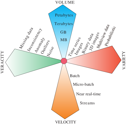
(b)

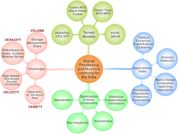
Figure 1.1: A framework for extremely large-scale data analysis. (a) The 4V challenges for big data. (b) A unified framework for the 4V challenges and the potential applications based on tensor decomposition approaches.

Owing to the increasingly affordable recording devices, extreme-scale volumes and variety of data are becoming ubiquitous across the science and engineering disciplines. In the case of multimedia (speech, video), remote sensing and medical / biological data, the analysis also requires a paradigm shift in order to efficiently process massive datasets within tolerable time (velocity). Such massive datasets may have billions of entries and are typically represented in the form of huge block matrices and/or tensors. This has spurred a renewed interest in the development of matrix / tensor algorithms that are suitable for very large-scale datasets. We show that tensor networks provide a natural sparse and distributed representation for big data, and address both established and emerging methodologies for tensor-based representations and optimization. Our particular focus is on low-rank tensor network representations, which allow for huge data tensors to be approximated (compressed) by interconnected low-order core tensors.

1.2 Tensor Notations and Graphical Representations

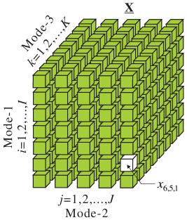
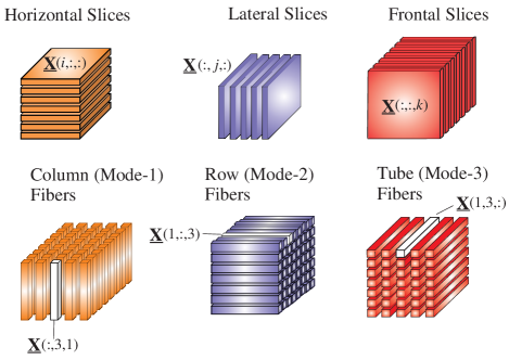
Figure 1.2: A 3rd-order tensor $\underline{{\bf X}}\in\mathbb{R}^{I\times J\times K}$, with entries $x_{i,j,k}=\underline{{\bf X}}(i,j,k)$, and its subtensors: slices (middle) and fibers (bottom). All fibers are treated as column vectors.

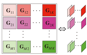
Figure 1.3: A block matrix and its representation as a 4th-order tensor, created by reshaping (or a projection) of blocks in the rows into lateral slices of 3rd-order tensors.

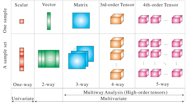
Figure 1.4: Graphical representation of multiway array (tensor) data of increasing structural complexity and “Volume” (see [155] for more detail).

Tensors are multi-dimensional generalizations of matrices. A matrix (2nd-order tensor) has two modes, rows and columns, while an $N$th-order tensor has $N$ modes (see Figures 1.2–1.7); for example, a 3rd-order tensor (with three-modes) looks like a cube (see Figure 1.2). Subtensors are formed when a subset of tensor indices is fixed. Of particular interest are fibers which are vectors obtained by fixing every tensor index but one, and matrix slices which are two-dimensional sections (matrices) of a tensor, obtained by fixing all the tensor indices but two. It should be noted that block matrices can also be represented by tensors, as illustrated in Figure 1.3 for 4th-order tensors.

We adopt the notation whereby tensors (for $N\geq 3$) are denoted by bold underlined capital letters, e.g., $\underline{{\bf X}}\in\mathbb{R}^{I_{1}\times I_{2}\times\cdots\times I_{N}}$. For simplicity, we assume that all tensors are real-valued, but it is, of course, possible to define tensors as complex-valued or over arbitrary fields. Matrices are denoted by boldface capital letters, e.g., ${\bf X}\in\mathbb{R}^{I\times J}$, and vectors (1st-order tensors) by boldface lower case letters, e.g., ${\bf x}\in\mathbb{R}^{J}$. For example, the columns of the matrix ${\bf A}=[{\bf a}_{1},{\bf a}_{2},\ldots,{\bf a}_{R}]\in\mathbb{R}^{I\times R}$ are the vectors denoted by ${\bf a}_{r}\in\mathbb{R}^{I}$, while the elements of a matrix (scalars) are denoted by lowercase letters, e.g., $a_{ir}={\bf A}(i,r)$ (see Table 1.1).

A specific entry of an $N$th-order tensor $\underline{{\bf X}}\in\mathbb{R}^{I_{1}\times I_{2}\times\cdots\times I_{N}}$ is denoted by $x_{i_{1},i_{2},\ldots,i_{N}}=\underline{{\bf X}}(i_{1},i_{2},\ldots,i_{N})\in\mathbb{R}$. The order of a tensor is the number of its “modes”, “ways” or “dimensions”, which can include space, time, frequency, trials, classes, and dictionaries. The term ‘‘size” stands for the number of values that an index can take in a particular mode. For example, the tensor $\underline{{\bf X}}\in\mathbb{R}^{I_{1}\times I_{2}\times\cdots\times I_{N}}$ is of order $N$ and size $I_{n}$ in all modes-$n$ $(n=1,2,\ldots,N)$. Lower-case letters e.g, $i,j$ are used for the subscripts in running indices and capital letters $I,J$ denote the upper bound of an index, i.e., $i=1,2,\ldots,I$ and $j=1,2,\ldots,J$. For a positive integer $n$, the shorthand notation $<n>$ denotes the set of indices $\{1,2,\ldots,n\}$.

Table 1.1: Basic matrix/tensor notation and symbols.

$\underline{{\bf X}}\in\mathbb{R}^{I_{1}\times I_{2}\times\cdots\times I_{N}}$ $N$th-order tensor of size $I_{1}\times I_{2}\times\cdots\times I_{N}$ $x_{i_{1},i_{2},\ldots,i_{N}}=\underline{{\bf X}}(i_{1},i_{2},\ldots,i_{N})$ $(i_{1},i_{2},\ldots,i_{N})$th entry of $\underline{{\bf X}}$ $x,\;{\bf x},\;{\bf X}$ scalar, vector and matrix $\underline{{\bf G}},\;\underline{{\bf S}},\;\underline{{\bf G}}^{(n)},\;\underline{{\bf X}}^{(n)}$ core tensors $\underline{\mbox{\boldmath$\Lambda$}}\in\mathbb{R}^{R\times R\times\cdots\times R}$ $N$th-order diagonal core tensor with nonzero entries $\lambda_{r}$ on the main diagonal ${{\bf A}}^{\text{T}}$, ${{\bf A}}^{-1}$, ${{\bf A}}^{{\dagger}}$ transpose, inverse and Moore–Penrose pseudo-inverse of a matrix ${\bf A}$ ${\bf A}=[{\bf a}_{1},{\bf a}_{2},\ldots,{\bf a}_{R}]\in\mathbb{R}^{I\times R}$ matrix with $R$ column vectors ${\bf a}_{r}\in\mathbb{R}^{I}$, with entries $a_{ir}$ ${\bf A},\,{\bf B},\,{\bf C},\;{\bf A}^{(n)},{\bf B}^{(n)},\;{\bf U}^{(n)}$ component (factor) matrices ${\bf X}_{(n)}\in\mathbb{R}^{I_{n}\times I_{1}\cdots I_{n-1}I_{n+1}\cdots I_{N}}$ mode-$n$ matricization of $\underline{{\bf X}}\in\mathbb{R}^{I_{1}\times\cdots\times I_{N}}$ ${\bf X}_{<n>}\in\mathbb{R}^{I_{1}I_{2}\cdots I_{n}\times I_{n+1}\cdots I_{N}}$ mode-($1,\ldots,n$) matricization of $\underline{{\bf X}}\in\mathbb{R}^{I_{1}\times\cdots\times I_{N}}$ $\underline{{\bf X}}({:,i_{2},i_{3},\ldots,i_{N}})\in\mathbb{R}^{I_{1}}$ mode-1 fiber of a tensor $\underline{{\bf X}}$ obtained by fixing all indices but one (a vector) $\underline{{\bf X}}({:,:,i_{3},\ldots,i_{N}})\in\mathbb{R}^{I_{1}\times I_{2}}$ slice (matrix) of a tensor $\underline{{\bf X}}$ obtained by fixing all indices but two $\underline{{\bf X}}({:,:,:,i_{4},\ldots,i_{N}})$ subtensor of $\underline{{\bf X}}$, obtained by fixing several indices $R,\;(R_{1},\ldots,R_{N})$ tensor rank $R$ and multilinear rank $\circ\;,\;\odot\;,\;\otimes$ $\otimes_{L}\>,\;\,|\!\!\otimes\!\!|\,$ outer, Khatri–Rao, Kronecker products Left Kronecker, strong Kronecker products ${\bf x}=\operatorname{vec}\left(\underline{{\bf X}}\right)$ vectorization of $\underline{{\bf X}}$ $\mathop{\rm tr}\nolimits(\bullet)$ trace of a square matrix $\mathop{\rm diag}\nolimits(\bullet)$ diagonal matrix

Table 1.2: Terminology used for tensor networks across the machine learning / scientific computing and quantum physics / chemistry communities.

Machine Learning Quantum Physics $N$th-order tensor rank-$N$ tensor high/low-order tensor tensor of high/low dimension ranks of TNs bond dimensions of TNs unfolding, matricization grouping of indices tensorization splitting of indices core site variables open (physical) indices ALS Algorithm one-site DMRG or DMRG1 MALS Algorithm two-site DMRG or DMRG2 column vector ${\bf x}\in\mathbb{R}^{I\times 1}$ ket $|\Psi\rangle$ row vector ${\bf x}^{\text{T}}\in\mathbb{R}^{1\times I}$ bra $\langle\Psi|$ inner product $\langle{\bf x},{\bf x}\rangle={\bf x}^{\text{T}}{\bf x}$ $\langle\Psi|\Psi\rangle$ Tensor Train (TT) Matrix Product State (MPS) (with Open Boundary Conditions (OBC)) Tensor Chain (TC) MPS with Periodic Boundary Conditions (PBC) Matrix TT Matrix Product Operators (with OBC) Hierarchical Tucker (HT) Tree Tensor Network State (TTNS) with rank-3 tensors

(a)

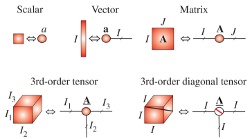
(b)

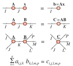
Figure 1.5: Graphical representation of tensor manipulations. (a) Basic building blocks for tensor network diagrams. (b) Tensor network diagrams for matrix-vector multiplication (top), matrix by matrix multiplication (middle) and contraction of two tensors (bottom). The order of reading of indices is anti-clockwise, from the left position.

Notations and terminology used for tensors and tensor networks differ across the scientific communities (see Table 1.2); to this end we employ a unifying notation particularly suitable for machine learning and signal processing research, which is summarized in Table 1.1.

Even with the above notation conventions, a precise description of tensors and tensor operations is often tedious and cumbersome, given the multitude of indices involved. To this end, in this monograph, we grossly simplify the description of tensors and their mathematical operations through diagrammatic representations borrowed from physics and quantum chemistry (see [156] and references therein). In this way, tensors are represented graphically by nodes of any geometrical shapes (e.g., circles, squares, dots), while each outgoing line (“edge”, “leg”,“arm”) from a node represents the indices of a specific mode (see Figure 1.5(a)). In our adopted notation, each scalar (zero-order tensor), vector (first-order tensor), matrix (2nd-order tensor), 3rd-order tensor or higher-order tensor is represented by a circle (or rectangular), while the order of a tensor is determined by the number of lines (edges) connected to it. According to this notation, an $N$th-order tensor $\underline{{\bf X}}\in\mathbb{R}^{I_{1}\times\cdots\times I_{N}}$ is represented by a circle (or any shape) with $N$ branches each of size $I_{n},\;n=1,2,\ldots,N$ (see Section 2). An interconnection between two circles designates a contraction of tensors, which is a summation of products over a common index (see Figure 1.5(b) and Section 2).

4th-order tensor

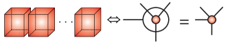
5th-order tensors
 
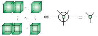
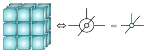
6th-order tensor

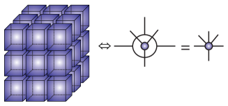
Figure 1.6: Graphical representations and symbols for higher-order block tensors. Each block represents either a 3rd-order tensor or a 2nd-order tensor. The outer circle indicates a global structure of the block tensor (e.g. a vector, a matrix, a 3rd-order block tensor), while the inner circle reflects the structure of each element within the block tensor. For example, in the top diagram a vector of 3rd order tensors is represented by an outer circle with one edge (a vector) which surrounds an inner circle with three edges (a 3rd order tensor), so that the whole structure designates a 4th-order tensor.

Block tensors, where each entry (e.g., of a matrix or a vector) is an individual subtensor, can be represented in a similar graphical form, as illustrated in Figure 1.6. Hierarchical (multilevel block) matrices are also naturally represented by tensors and vice versa, as illustrated in Figure 1.7 for 4th-, 5th- and 6th-order tensors. All mathematical operations on tensors can be therefore equally performed on block matrices.

In this monograph, we make extensive use of tensor network diagrams as an intuitive and visual way to efficiently represent tensor decompositions. Such graphical notations are of great help in studying and implementing sophisticated tensor operations. We highlight the significant advantages of such diagrammatic notations in the description of tensor manipulations, and show that most tensor operations can be visualized through changes in the architecture of a tensor network diagram.

(a)

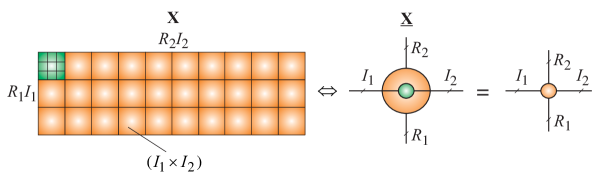
(b)

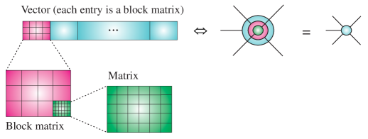
(c)

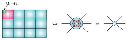
Figure 1.7: Hierarchical matrix structures and their symbolic representation as tensors. (a) A 4th-order tensor representation for a block matrix ${\bf X}\in\mathbb{R}^{R_{1}I_{1}\times R_{2}I_{2}}$ (a matrix of matrices), which comprises block matrices ${\bf X}_{r_{1},r_{2}}\in\mathbb{R}^{I_{1}\times I_{2}}$. (b) A 5th-order tensor. (c) A 6th-order tensor.

1.3 Curse of Dimensionality and Generalized Separation of Variables for Multivariate Functions

1.3.1 Curse of Dimensionality

The term curse of dimensionality was coined by [18] to indicate that the number of samples needed to estimate an arbitrary function with a given level of accuracy grows exponentially with the number of variables, that is, with the dimensionality of the function. In a general context of machine learning and the underlying optimization problems, the “curse of dimensionality” may also refer to an exponentially increasing number of parameters required to describe the data/system or an extremely large number of degrees of freedom. The term “curse of dimensionality”, in the context of tensors, refers to the phenomenon whereby the number of elements, $I^{N}$, of an $N$th-order tensor of size $(I\times I\times\cdots\times I)$ grows exponentially with the tensor order, $N$. Tensor volume can therefore easily become prohibitively big for multiway arrays for which the number of dimensions (“ways” or “modes”) is very high, thus requiring enormous computational and memory resources to process such data. The understanding and handling of the inherent dependencies among the excessive degrees of freedom create both difficult to solve problems and fascinating new opportunities, but comes at a price of reduced accuracy, owing to the necessity to involve various approximations.

We show that the curse of dimensionality can be alleviated or even fully dealt with through tensor network representations; these naturally cater for the excessive volume, veracity and variety of data (see Figure 1.1) and are supported by efficient tensor decomposition algorithms which involve relatively simple mathematical operations. Another desirable aspect of tensor networks is their relatively small-scale and low-order core tensors, which act as “building blocks” of tensor networks. These core tensors are relatively easy to handle and visualize, and enable super-compression of the raw, incomplete, and noisy huge-scale datasets. This also suggests a solution to a more general quest for new technologies for processing of exceedingly large datasets within affordable computation times.

To address the curse of dimensionality, this work mostly focuses on approximative low-rank representations of tensors, the so-called low-rank tensor approximations (LRTA) or low-rank tensor network decompositions.

1.4 Separation of Variables and Tensor Formats

A tensor is said to be in a full format when it is represented as an original (raw) multidimensional array [118], however, distributed storage and processing of high-order tensors in their full format is infeasible due to the curse of dimensionality. The sparse format is a variant of the full tensor format which stores only the nonzero entries of a tensor, and is used extensively in software tools such as the Tensor Toolbox [8] and in the sparse grid approach [80, 25, 91].

As already mentioned, the problem of huge dimensionality can be alleviated through various distributed and compressed tensor network formats, achieved by low-rank tensor network approximations. The underpinning idea is that by employing tensor networks formats, both computational costs and storage requirements may be dramatically reduced through distributed storage and computing resources. It is important to note that, except for very special data structures, a tensor cannot be compressed without incurring some compression error, since a low-rank tensor representation is only an approximation of the original tensor.

The concept of compression of multidimensional large-scale data by tensor network decompositions can be intuitively explained as follows. Consider the approximation of an $N$-variate function $f({\bf x})=f(x_{1},x_{2},\ldots,x_{N})$ by a finite sum of products of individual functions, each depending on only one or a very few variables [16, 67, 34, 206]. In the simplest scenario, the function $f({\bf x})$ can be (approximately) represented in the following separable form

$$f(x_{1},x_{2},\ldots,x_{N})\cong f^{(1)}(x_{1})f^{(2)}(x_{2})\cdots f^{(N)}(x_{N}).$$ (1.1)

In practice, when an $N$-variate function $f({\bf x})$ is discretized into an $N$th-order array, or a tensor, the approximation in (1.1) then corresponds to the representation by rank-1 tensors, also called elementary tensors (see Section 2). Observe that with $I_{n},\;n=1,2,\ldots,N$ denoting the size of each mode and $I=\max_{n}\{I_{n}\}$, the memory requirement to store such a full tensor is $\prod_{n=1}^{N}I_{n}\leq I^{N}$, which grows exponentially with $N$. On the other hand, the separable representation in (1.1) is completely defined by its factors, $f^{(n)}(x_{n}),\;(n=1,2,\ldots,N$), and requires only $\sum_{n=1}^{N}I_{n}\ll I^{N}$ storage units. If $x_{1},x_{2},\ldots,x_{N}$ are statistically independent random variables, their joint probability density function is equal to the product of marginal probabilities, $f({\bf x})=f^{(1)}(x_{1})f^{(2)}(x_{2})\cdots f^{(N)}(x_{N})$, in an exact analogy to outer products of elementary tensors. Unfortunately, the form of separability in (1.1) is rather rare in practice.

The concept of tensor networks rests upon generalized (full or partial) separability of the variables of a high dimensional function. This can be achieved in different tensor formats, including:

• The Canonical Polyadic (CP) format (see Section 3.2), where

  $$f(x_{1},x_{2},\ldots,x_{N})\cong\sum_{r=1}^{R}f_{r}^{(1)}(x_{1})\,f_{r}^{(2)}(x_{2})\cdots f_{r}^{(N)}(x_{N}),$$ (1.2)

  in an exact analogy to (1.1). In a discretized form, the above CP format can be written as an $N$th-order tensor

  $$\underline{{\bf F}}\cong\sum_{r=1}^{R}{{\bf f}}_{\;r}^{(1)}\circ{{\bf f}}_{\;r}^{(2)}\circ\cdots\circ{{\bf f}}_{\;r}^{(N)}\in\mathbb{R}^{I_{1}\times I_{2}\times\cdots\times I_{N}},$$ (1.3)

  where ${{\bf f}}_{\;r}^{(n)}\in\mathbb{R}^{I_{n}}$ denotes a discretized version of the univariate function $f_{r}^{(n)}(x_{n})$, symbol $\circ$ denotes the outer product, and $R$ is the tensor rank.

• The Tucker format, given by

  $$f(x_{1},\ldots,x_{N})\cong\sum_{r_{1}=1}^{R_{1}}\cdots\sum_{r_{N}=1}^{R_{N}}g_{r_{1},\ldots,r_{N}}\;f_{r_{1}}^{(1)}(x_{1})\cdots f_{r_{N}}^{(N)}(x_{N}),$$ (1.4)

  and its distributed tensor network variants (see Section 3.3),

• The Tensor Train (TT) format (see Section 4.1), in the form

  $$f(x_{1},x_{2},\ldots,x_{N}) \cong \sum_{r_{1}=1}^{R_{1}}\sum_{r_{2}=1}^{R_{2}}\cdots\sum_{r_{N-1}=1}^{R_{N-1}}f_{r_{1}}^{(1)}(x_{1})\,f_{r_{1}\,r_{2}}^{(2)}(x_{2})\cdots$$ (1.5)

  $$\cdots f_{r_{N-2}\,r_{N-1}}^{(N-2)}(x_{N-1})\;f_{r_{N-1}}^{(N)}(x_{N}),$$

  with the equivalent compact matrix representation

  $$f(x_{1},x_{2},\ldots,x_{N})\cong{\bf F}^{(1)}(x_{1})\,{\bf F}^{(2)}(x_{2})\cdots{\bf F}^{(N)}(x_{N}),$$ (1.6)

  where ${\bf F}^{(n)}(x_{n})\in\mathbb{R}^{R_{n-1}\times R_{n}}$, with $R_{0}=R_{N}=1$.

• The Hierarchical Tucker (HT) format (also known as the Hierarchical Tensor format) can be expressed via a hierarchy of nested separations in the following way. Consider nested nonempty disjoint subsets $u$, $v$, and $t=u\cup v\subset\{1,2,\ldots,N\}$, then for some $1\leq N_{0}<N$, with $u_{0}=\{1,\ldots,N_{0}\}$ and $v_{0}=\{N_{0}+1,\ldots,N\}$, the HT format can be expressed as

  $$f(x_{1},\ldots,x_{N}) \cong \sum_{r_{u_{0}}=1}^{R_{u_{0}}}\sum_{r_{v_{0}}=1}^{R_{v_{0}}}g^{(12\cdots N)}_{r_{u_{0}},r_{v_{0}}}\,f^{({u_{0}})}_{r_{u_{0}}}({\bf x}_{u_{0}})\,f^{({v_{0}})}_{r_{v_{0}}}({\bf x}_{v_{0}}),$$

  $$f^{(t)}_{r_{t}}({\bf x}_{t}) \cong \sum_{r_{u}=1}^{R_{u}}\sum_{r_{v}=1}^{R_{v}}g^{(t)}_{r_{u},r_{v},r_{t}}\,f^{(u)}_{r_{u}}({\bf x}_{u})\,f^{(v)}_{r_{v}}({\bf x}_{v}),$$

  where ${\bf x}_{t}=\{x_{i}:i\in t\}$. See Section 2.3 for more detail.

  Example. In a particular case for $N$=4, the HT format can be expressed by

  $$f(x_{1},x_{2},x_{3},x_{4}) \cong \sum_{r_{12}=1}^{R_{12}}\sum_{r_{34}=1}^{R_{34}}g^{(1234)}_{r_{12},r_{34}}\,f^{(12)}_{r_{12}}(x_{1},x_{2})\,f^{(34)}_{r_{34}}(x_{3},x_{4}),$$

  $$f^{(12)}_{r_{12}}(x_{1},x_{2}) \cong \sum_{r_{1}=1}^{R_{1}}\sum_{r_{2}=1}^{R_{2}}g^{(12)}_{r_{1},r_{2},r_{12}}\,f^{(1)}_{r_{1}}(x_{1})\,f^{(2)}_{r_{2}}(x_{2}),$$

  $$f^{(34)}_{r_{34}}(x_{3},x_{4}) \cong \sum_{r_{3}=1}^{R_{3}}\sum_{r_{4}=1}^{R_{4}}g^{(34)}_{r_{3},r_{4},r_{34}}\,f^{(3)}_{r_{3}}(x_{3})\,f^{(4)}_{r_{4}}(x_{4}).$$

  The Tree Tensor Network States (TTNS) format, which is an extension of the HT format, can be obtained by generalizing the two subsets, $u,v$, into a larger number of disjoint subsets $u_{1},\ldots,u_{m}$, $m\geq 2$. In other words, the TTNS can be obtained by more flexible separations of variables through products of larger numbers of functions at each hierarchical level (see Section 2.3 for graphical illustrations and more detail).

All the above approximations adopt the form of “sum-of-products” of single-dimensional functions, a procedure which plays a key role in all tensor factorizations and decompositions.

Indeed, in many applications based on multivariate functions, very good approximations are obtained with a surprisingly small number of factors; this number corresponds to the tensor rank, $R$, or tensor network ranks, $\{R_{1},R_{2},\ldots,R_{N}\}$ (if the representations are exact and minimal). However, for some specific cases this approach may fail to obtain sufficiently good low-rank TN approximations. The concept of generalized separability has already been explored in numerical methods for high-dimensional density function equations [133, 206, 34] and within a variety of huge-scale optimization problems (see Part 2 of this monograph).

To illustrate how tensor decompositions address excessive volumes of data, if all computations are performed on a CP tensor format in (1.3) and not on the raw $N$th-order data tensor itself, then instead of the original, exponentially growing, data dimensionality of $I^{N}$, the number of parameters in a CP representation reduces to $NIR$, which scales linearly in the tensor order $N$ and size $I$ (see Table 4.4). For example, the discretization of a $5$-variate function over $100$ sample points on each axis would yield the difficulty to manage $100^{5}=10,000,000,000$ sample points, while a rank-$2$ CP representation would require only $5\times 2\times 100=1000$ sample points.

Although the CP format in (1.2) effectively bypasses the curse of dimensionality, the CP approximation may involve numerical problems for very high-order tensors, which in addition to the intrinsic uncloseness of the CP format (i.e., difficulty to arrive at a canonical format), the corresponding algorithms for CP decompositions are often ill-posed [63]. As a remedy, greedy approaches may be considered which, for enhanced stability, perform consecutive rank-1 corrections [135]. On the other hand, many efficient and stable algorithms exist for the more flexible Tucker format in (1.4), however, this format is not practical for tensor orders $N>5$ because the number of entries of both the original data tensor and the core tensor (expressed in (1.4) by elements $g_{r_{1},r_{2},\ldots,r_{N}}$) scales exponentially in the tensor order $N$ (curse of dimensionality).

In contrast to CP decomposition algorithms, TT tensor network formats in (1.5) exhibit both very good numerical properties and the ability to control the error of approximation, so that a desired accuracy of approximation is obtained relatively easily. The main advantage of the TT format over the CP decomposition is the ability to provide stable quasi-optimal rank reduction, achieved through, for example, truncated singular value decompositions (tSVD) or adaptive cross-approximation [162, 16, 116]. This makes the TT format one of the most stable and simple approaches to separate latent variables in a sophisticated way, while the associated TT decomposition algorithms provide full control over low-rank TN approximations. In this monograph, we therefore make extensive use of the TT format for low-rank TN approximations and employ the TT toolbox software for efficient implementations [160]. The TT format will also serve as a basic prototype for high-order tensor representations, while we also consider the Hierarchical Tucker (HT) and the Tree Tensor Network States (TTNS) formats (having more general tree-like structures) whenever advantageous in applications.

Furthermore, we address in depth the concept of tensorization of structured vectors and matrices to convert a wide class of huge-scale optimization problems into much smaller-scale interconnected optimization sub-problems which can be solved by existing optimization methods (see Part 2 of this monograph).

The tensor network optimization framework is therefore performed through the two main steps:

• Tensorization of data vectors and matrices into a high-order tensor, followed by a distributed approximate representation of a cost function in a specific low-rank tensor network format.

• Execution of all computations and analysis in tensor network formats (i.e., using only core tensors) that scale linearly, or even sub-linearly (quantized tensor networks), in the tensor order $N$. This yields both the reduced computational complexity and distributed memory requirements.

1.5 Advantages of Multiway Analysis via Tensor Networks

In this monograph, we focus on two main challenges in huge-scale data analysis which are addressed by tensor networks: (i) an approximate representation of a specific cost (objective) function by a tensor network while maintaining the desired accuracy of approximation, and (ii) the extraction of physically meaningful latent variables from data in a sufficiently accurate and computationally affordable way. The benefits of multiway (tensor) analysis methods for large-scale datasets then include:

• Ability to perform all mathematical operations in tractable tensor network formats;

• Simultaneous and flexible distributed representations of both the structurally rich data and complex optimization tasks;

• Efficient compressed formats of large multidimensional data achieved via tensorization and low-rank tensor decompositions into low-order factor matrices and/or core tensors;

• Ability to operate with noisy and missing data by virtue of numerical stability and robustness to noise of low-rank tensor / matrix approximation algorithms;

• A flexible framework which naturally incorporates various diversities and constraints, thus seamlessly extending the standard, flat view, Component Analysis (2-way CA) methods to multiway component analysis;

• Possibility to analyze linked (coupled) blocks of large-scale matrices and tensors in order to separate common / correlated from independent / uncorrelated components in the observed raw data;

• Graphical representations of tensor networks allow us to express mathematical operations on tensors (e.g., tensor contractions and reshaping) in a simple and intuitive way, and without the explicit use of complex mathematical expressions.

In that sense, this monograph both reviews current research in this area and complements optimisation methods, such as the Alternating Direction Method of Multipliers (ADMM) [23].

Tensor decompositions (TDs) have been already adopted in widely diverse disciplines, including psychometrics, chemometrics, biometric, quantum physics / information, quantum chemistry, signal and image processing, machine learning, and brain science [190, 202, 124, 119, 91, 79, 43, 42]. This is largely due to their advantages in the analysis of data that exhibit not only large volume but also very high variety (see Figure 1.1), as in the case in bio- and neuroinformatics and in computational neuroscience, where various forms of data collection include sparse tabular structures and graphs or hyper-graphs.

Moreover, tensor networks have the ability to efficiently parameterize, through structured compact representations, very general high-dimensional spaces which arise in modern applications [121, 39, 229, 50, 136, 116, 19]. Tensor networks also naturally account for intrinsic multidimensional and distributed patterns present in data, and thus provide the opportunity to develop very sophisticated models for capturing multiple interactions and couplings in data – these are more physically insightful and interpretable than standard pair-wise interactions.

1.6 Scope and Objectives

Review and tutorial papers [119, 137, 87, 42, 54, 189, 163, 7] and books [190, 124, 43, 91] dealing with TDs and TNs already exist, however, they typically focus on standard models, with no explicit links to very large-scale data processing topics or connections to a wide class of optimization problems. The aim of this monograph is therefore to extend beyond the standard Tucker and CP tensor decompositions, and to demonstrate the perspective of TNs in extremely large-scale data analytics, together with their role as a mathematical backbone in the discovery of hidden structures in prohibitively large-scale data. Indeed, we show that TN models provide a framework for the analysis of linked (coupled) blocks of tensors with millions and even billions of non-zero entries.

We also demonstrate that TNs provide natural extensions of 2-way (matrix) Component Analysis (2-way CA) methods to multi-way component analysis (MWCA), which deals with the extraction of desired components from multidimensional and multimodal data. This paradigm shift requires new models and associated algorithms capable of identifying core relations among the different tensor modes, while guaranteeing linear / sub-linear scaling with the size of datasets.

Furthermore, we review tensor decompositions and the associated algorithms for very large-scale linear / multilinear dimensionality reduction problems. The related optimization problems often involve structured matrices and vectors with over a billion entries (see [87, 67, 81] and references therein). In particular, we focus on Symmetric Eigenvalue Decomposition (EVD/PCA) and Generalized Eigenvalue Decomposition (GEVD) [70, 120, 123], SVD [127], solutions of overdetermined and undetermined systems of linear algebraic equations [159, 71], the Moore–Penrose pseudo-inverse of structured matrices [129], and Lasso problems [130]. Tensor networks for extremely large-scale multi-block (multi-view) data are also discussed, especially TN models for orthogonal Canonical Correlation Analysis (CCA) and related Partial Least Squares (PLS) problems. For convenience, all these problems are reformulated as constrained optimization problems which are then, by virtue of low-rank tensor networks reduced to manageable lower-scale optimization sub-problems. The enhanced tractability and scalability is achieved through tensor network contractions and other tensor network transformations.

The methods and approaches discussed in this work can be considered a both an alternative and complementary to other emerging methods for huge-scale optimization problems like random coordinate descent (RCD) scheme [150, 180], sub-gradient methods [151], alternating direction method of multipliers (ADMM) [23], and proximal gradient descent methods [165] (see also [30, 98] and references therein).

This monograph systematically introduces TN models and the associated algorithms for TNs/TDs and illustrates many potential applications of TDs/TNS. The dimensionality reduction and optimization frameworks (see Part 2 of this monograph) are considered in detail, and we also illustrate the use of TNs in other challenging problems for huge-scale datasets which can be solved using the tensor network approach, including anomaly detection, tensor completion, compressed sensing, clustering, and classification.

Chapter 2 Tensor Operations and Tensor Network Diagrams

Tensor operations benefit from the power of multilinear algebra which is structurally much richer than linear algebra, and even some basic properties, such as the rank, have a more complex meaning. We next introduce the background on fundamental mathematical operations in multilinear algebra, a prerequisite for the understanding of higher-order tensor decompositions. A unified account of both the definitions and properties of tensor network operations is provided, including the outer, multi-linear, Kronecker, and Khatri–Rao products. For clarity, graphical illustrations are provided, together with an example rich guidance for tensor network operations and their properties. To avoid any confusion that may arise given the numerous options on tensor reshaping, both mathematical operations and their properties are expressed directly in their native multilinear contexts, supported by graphical visualizations.

Table 2.1: Basic tensor/matrix operations.

$\underline{{\bf C}}=\underline{{\bf A}}\times_{n}{\bf B}$ Mode-$n$ product of a tensor $\underline{{\bf A}}\in\mathbb{R}^{I_{1}\times I_{2}\times\cdots\times I_{N}}$ and a matrix ${\bf B}\in\mathbb{R}^{J\times I_{n}}$ yields a tensor $\underline{{\bf C}}\in\mathbb{R}^{I_{1}\times\cdots\times I_{n-1}\times J\times I_{n+1}\times\cdots\times I_{N}}$, with entries $c_{\,i_{1},\ldots,i_{n-1},\,j,\,i_{n+1},\ldots,i_{N}}=\sum_{i_{n}=1}^{I_{n}}\;a_{i_{1},\ldots,i_{n},\ldots,i_{N}}\,b_{j,\,i_{n}}$ $\underline{{\bf C}}=\llbracket\underline{{\bf G}};{\bf B}^{(1)},\ldots,{\bf B}^{(N)}\rrbracket$ Multilinear (Tucker) product of a core tensor, $\underline{{\bf G}}$, and factor matrices ${\bf B}^{(n)}$, which gives $\underline{{\bf C}}=\underline{{\bf G}}\times_{1}{\bf B}^{(1)}\times_{2}{\bf B}^{(2)}\cdots\times_{N}{\bf B}^{(N)}$ $\underline{{\bf C}}=\underline{{\bf A}}\,\bar{\times}_{n}\;{\bf b}$ Mode-$n$ product of a tensor $\underline{{\bf A}}\in\mathbb{R}^{I_{1}\times\cdots\times I_{N}}$ and vector ${\bf b}\in\mathbb{R}^{I_{n}}$ yields a tensor $\underline{{\bf C}}\in\mathbb{R}^{I_{1}\times\cdots\times I_{n-1}\times I_{n+1}\times\cdots\times I_{N}}$, with entries $c_{\,i_{1},\ldots,i_{n-1},i_{n+1},\ldots,i_{N}}=\sum_{i_{n}=1}^{I_{n}}a_{i_{1},\ldots,i_{n-1},i_{n},i_{n+1},\ldots,i_{N}}\;b_{i_{n}}$ $\underline{{\bf C}}=\underline{{\bf A}}\times_{N}^{1}\underline{{\bf B}}=\underline{{\bf A}}\times^{1}\underline{{\bf B}}$ Mode-$(N,1)$ contracted product of tensors $\underline{{\bf A}}\in\mathbb{R}^{I_{1}\times I_{2}\times\cdots\times I_{N}}$ and $\underline{{\bf B}}\in\mathbb{R}^{J_{1}\times J_{2}\times\cdots\times J_{M}}$, with $I_{N}=J_{1}$, yields a tensor $\underline{{\bf C}}\in\mathbb{R}^{I_{1}\times\cdots\times I_{N-1}\times J_{2}\times\cdots\times J_{M}}$ with entries $c_{i_{1},\ldots,i_{N-1},j_{2},\ldots,j_{M}}=\sum_{i_{N}=1}^{I_{N}}a_{i_{1},\ldots,i_{N}}\;b_{i_{N},j_{2},\ldots,j_{M}}$ $\underline{{\bf C}}=\underline{{\bf A}}\circ\underline{{\bf B}}$ Outer product of tensors $\underline{{\bf A}}\in\mathbb{R}^{I_{1}\times I_{2}\times\cdots\times I_{N}}$ and $\underline{{\bf B}}\in\mathbb{R}^{J_{1}\times J_{2}\times\cdots\times J_{M}}$ yields an $(N+M)$th-order tensor $\underline{{\bf C}}$, with entries $c_{\;i_{1},\ldots,i_{N},\,j_{1},\ldots,j_{M}}=a_{i_{1},\ldots,i_{N}}\;b_{j_{1},\ldots,j_{M}}$ $\underline{{\bf X}}={\bf a}\circ{\bf b}\circ{\bf c}\in\mathbb{R}^{I\times J\times K}$ Outer product of vectors ${\bf a},{\bf b}$ and ${\bf c}$ forms a rank-1 tensor, $\underline{{\bf X}}$, with entries $x_{ijk}=a_{i}\;b_{j}\;c_{k}$ $\underline{{\bf C}}=\underline{{\bf A}}\otimes_{L}\underline{{\bf B}}$ (Left) Kronecker product of tensors $\underline{{\bf A}}\in\mathbb{R}^{I_{1}\times I_{2}\times\cdots\times I_{N}}$ and $\underline{{\bf B}}\in\mathbb{R}^{J_{1}\times J_{2}\times\cdots\times J_{N}}$ yields a tensor $\underline{{\bf C}}\in\mathbb{R}^{I_{1}J_{1}\times\cdots\times I_{N}J_{N}}$, with entries $c_{\;\overline{i_{1}j_{1}},\ldots,\overline{i_{N}j_{N}}}=a_{i_{1},\ldots,i_{N}}\>b_{j_{1},\ldots,j_{N}}$ ${\bf C}={\bf A}\odot_{L}{\bf B}$ (Left) Khatri–Rao product of matrices ${\bf A}=[{\bf a}_{1},\ldots,{\bf a}_{J}]\in\mathbb{R}^{I\times J}$ and ${\bf B}=[{\bf b}_{1},\ldots,{\bf b}_{J}]\in\mathbb{R}^{K\times J}$ yields a matrix ${\bf C}\in\mathbb{R}^{IK\times J}$, with columns ${\bf c}_{j}={\bf a}_{j}\otimes_{L}{\bf b}_{j}\in\mathbb{R}^{IK}$

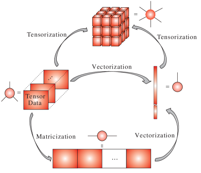
Figure 2.1: Tensor reshaping operations: Matricization, vectorization and tensorization. Matricization refers to converting a tensor into a matrix, vectorization to converting a tensor or a matrix into a vector, while tensorization refers to converting a vector, a matrix or a low-order tensor into a higher-order tensor.

2.1 Basic Multilinear Operations

The following symbols are used for most common tensor multiplications: $\otimes$ for the Kronecker product, $\odot$ for the Khatri–Rao product, $\circledast$ for the Hadamard (componentwise) product, $\circ$ for the outer product and $\times_{n}$ for the mode-$n$ product. Basic tensor operations are summarized in Table 2.1, and illustrated in Figures 2.1–2.13. We refer to [119, 43, 128] for more detail regarding the basic notations and tensor operations. For convenience, general operations, such as $\mbox{vec}(\cdot)$ or $\mathop{\rm diag}\nolimits(\cdot)$, are defined similarly to the MATLAB syntax.

Multi–indices: By a multi-index $i=\overline{i_{1}i_{2}\cdots i_{N}}$ we refer to an index which takes all possible combinations of values of indices, $i_{1},i_{2},\ldots,i_{N}$, for $i_{n}=1,2,\ldots,I_{n}$, $\;n=1,2,\ldots,N$ and in a specific order. Multi–indices can be defined using two different conventions [71]:

1. Little-endian convention (reverse lexicographic ordering)

   $$\overline{i_{1}i_{2}\cdots i_{N}}=i_{1}+(i_{2}-1)I_{1}+(i_{3}-1)I_{1}I_{2}+\cdots+(i_{N}-1)I_{1}\cdots I_{N-1}.$$

2. Big-endian (colexicographic ordering)

   $$\overline{i_{1}i_{2}\cdots i_{N}} = i_{N}+(i_{N-1}-1)I_{N}+(i_{N-2}-1)I_{N}I_{N-1}+$$

   $$\cdots+(i_{1}-1)I_{2}\cdots I_{N}.$$

The little-endian convention is used, for example, in Fortran and MATLAB, while the big-endian convention is used in C language. Given the complex and non-commutative nature of tensors, the basic definitions, such as the matricization, vectorization and the Kronecker product, should be consistent with the chosen convention. In this monograph, unless otherwise stated, we will use little-endian notation.

Matricization. The matricization operator, also known as the unfolding or flattening, reorders the elements of a tensor into a matrix (see Figure 2.2). Such a matrix is re-indexed according to the choice of multi-index described above, and the following two fundamental matricizations are used extensively.

The mode-$n$ matricization. For a fixed index $n\in\{1,2,\ldots,N\}$, the mode-$n$ matricization of an $N$th-order tensor, $\underline{{\bf X}}\in\mathbb{R}^{I_{1}\times\cdots\times I_{N}}$, is defined as the (“short” and “wide”) matrix

$${\bf X}_{(n)}\in\mathbb{R}^{I_{n}\times I_{1}I_{2}\cdots I_{n-1}I_{n+1}\cdots I_{N}},$$ (2.1)

with $I_{n}$ rows and $I_{1}I_{2}\cdots I_{n-1}I_{n+1}\cdots I_{N}$ columns, the entries of which are

$$({\bf X}_{(n)})_{i_{n},\overline{i_{1}\cdots i_{n-1}i_{n+1}\cdots i_{N}}}=x_{i_{1},i_{2},\ldots,i_{N}}.$$

Note that the columns of a mode-$n$ matricization, ${\bf X}_{(n)}$, of a tensor $\underline{{\bf X}}$ are the mode-$n$ fibers of $\underline{{\bf X}}$.

(a)

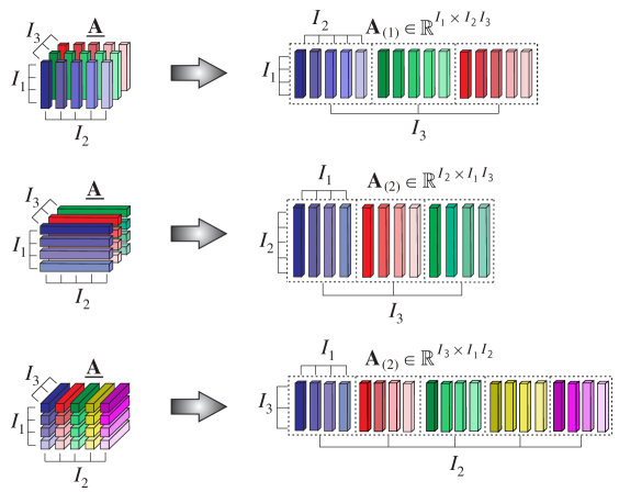
(b)

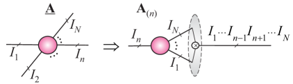
(c)

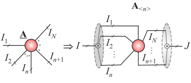
Figure 2.2: Matricization (flattening, unfolding) used in tensor reshaping. (a) Mode-1, mode-2, and mode-3 matricizations of a 3rd-order tensor, from the top to the bottom panel. (b) Tensor network diagram for the mode-$n$ matricization of an $N$th-order tensor, $\underline{{\bf A}}\in\mathbb{R}^{I_{1}\times I_{2}\times\cdots\times I_{N}}$, into a short and wide matrix, ${\bf A}_{(n)}\in\mathbb{R}^{I_{n}\;\times\;I_{1}\cdots I_{n-1}I_{n+1}\cdots I_{N}}$. (c) Mode-$\{1,2,\ldots,n\}$th (canonical) matricization of an $N$th-order tensor, $\underline{{\bf A}}$, into a matrix ${\bf A}_{<n>}={\bf A}_{(\overline{i_{1}\cdots i_{n}}\;;\;\overline{i_{n+1}\cdots i_{N}})}\in\mathbb{R}^{I_{1}I_{2}\cdots I_{n}\;\times\;I_{n+1}\cdots I_{N}}$.

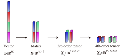
Figure 2.3: Tensorization of a vector into a matrix, 3rd-order tensor and 4th-order tensor.

The mode-$\{n\}$ canonical matricization. For a fixed index $n\in\{1,2,\ldots,N\}$, the mode-$(1,2,\ldots,n)$ matricization, or simply mode-$n$ canonical matricization, of a tensor $\underline{{\bf X}}\in\mathbb{R}^{I_{1}\times\cdots\times I_{N}}$ is defined as the matrix

$${\bf X}_{<n>}\in\mathbb{R}^{I_{1}I_{2}\cdots I_{n}\times I_{n+1}\cdots I_{N}},$$ (2.2)

with $I_{1}I_{2}\cdots I_{n}$ rows and $I_{n+1}\cdots I_{N}$ columns, and the entries

$$({\bf X}_{<n>})_{\overline{i_{1}i_{2}\cdots i_{n}},\,\overline{i_{n+1}\cdots i_{N}}}=x_{i_{1},i_{2},\ldots,i_{N}}.$$

The matricization operator in the MATLAB notation (reverse lexicographic) is given by

$${\bf X}_{<n>}=\mbox{reshape}\left(\underline{{\bf X}},I_{1}I_{2}\cdots I_{n},I_{n+1}\cdots I_{N}\right).$$ (2.3)

As special cases we immediately have (see Figure 2.2)

$${\bf X}_{<1>}={\bf X}_{(1)},\quad{\bf X}_{<N-1>}={\bf X}^{\text{T}}_{(N)},\quad{\bf X}_{<N>}=\text{vec}({\bf X}).$$ (2.4)

The tensorization of a vector or a matrix can be considered as a reverse process to the vectorization or matricization (see Figures  2.1 and 2.3).

Kronecker, strong Kronecker, and Khatri–Rao products of matrices and tensors. For an $I\times J$ matrix ${\bf A}$ and a $K\times L$ matrix ${\bf B}$, the standard (Right) Kronecker product, ${\bf A}\otimes{\bf B}$, and the Left Kronecker product, ${\bf A}\otimes_{L}{\bf B}$, are the following $IK\times JL$ matrices

$${\bf A}\otimes{\bf B}=\left[\begin{matrix}a_{1,1}{\bf B}&\cdots&a_{1,J}{\bf B}\\ \vdots&\ddots&\vdots\\ a_{I,1}{\bf B}&\cdots&a_{I,J}{\bf B}\end{matrix}\right],\quad{\bf A}\otimes_{L}{\bf B}=\left[\begin{matrix}{\bf A}b_{1,1}&\cdots&{\bf A}b_{1,L}\\ \vdots&\ddots&\vdots\\ {\bf A}b_{K,1}&\cdots&{\bf A}b_{K,L}\end{matrix}\right].$$

Observe that ${\bf A}\otimes_{L}{\bf B}={\bf B}\otimes{\bf A}$, so that the Left Kronecker product will be used in most cases in this monograph as it is consistent with the little-endian notation.

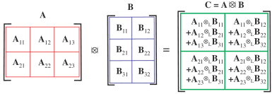
Figure 2.4: Illustration of the strong Kronecker product of two block matrices, ${\bf A}=[{\bf A}_{r_{1},r_{2}}]\in\mathbb{R}^{R_{1}I_{1}\times R_{2}J_{1}}$ and ${\bf B}=[{\bf B}_{r_{2},r_{3}}]\in\mathbb{R}^{R_{2}I_{2}\times R_{3}J_{2}}$, which is defined as a block matrix ${\bf C}={\bf A}\,|\!\!\otimes\!\!|\,{\bf B}\in\mathbb{R}^{R_{1}I_{1}I_{2}\times R_{3}J_{1}J_{2}}$, with the blocks ${\bf C}_{r_{1},r_{3}}=\sum_{r_{2}=1}^{R_{2}}{\bf A}_{r_{1},r_{2}}\otimes_{L}{\bf B}_{r_{2},r_{3}}\in\mathbb{R}^{I_{1}I_{2}\times J_{1}J_{2}}$, for $r_{1}=1,\ldots,R_{1},\;r_{2}=1,\ldots,R_{2}$ and $r_{3}=1,\ldots,R_{3}$.

Using Left Kronecker product, the strong Kronecker product of two block matrices, ${\bf A}\in\mathbb{R}^{R_{1}I\times R_{2}J}$ and ${\bf B}\in\mathbb{R}^{R_{2}K\times R_{3}L}$, given by

$${{\bf A}}=\begin{bmatrix}{\bf A}_{1,1}&\cdots&{\bf A}_{1,R_{2}}\\ \vdots&\ddots&\vdots\\ {\bf A}_{R_{1},1}&\cdots&{\bf A}_{R_{1},R_{2}}\end{bmatrix},\qquad{{\bf B}}=\begin{bmatrix}\ {\bf B}_{1,1}&\cdots&{\bf B}_{1,R_{3}}\\ \vdots&\ddots&\vdots\\ {\bf B}_{R_{2},1}&\cdots&{\bf B}_{R_{2},R_{3}}\end{bmatrix},$$

can be defined as a block matrix (see Figure 2.4 for a graphical illustration)

$${\bf C}={{\bf A}}\;\,|\!\!\otimes\!\!|\,\;{{\bf B}}\in\mathbb{R}^{R_{1}IK\times R_{3}JL},$$ (2.5)

with blocks ${\bf C}_{r_{1},r_{3}}=\sum_{r_{2}=1}^{R_{2}}{\bf A}_{r_{1},r_{2}}\otimes_{L}{\bf B}_{r_{2},r_{3}}\in\mathbb{R}^{IK\times JL}$, where ${\bf A}_{r_{1},r_{2}}\in\mathbb{R}^{I\times J}$ and ${\bf B}_{r_{2},r_{3}}\in\mathbb{R}^{K\times L}$ are the blocks of matrices within ${{\bf A}}$ and ${{\bf B}}$, respectively [62, 112, 113]. Note that the strong Kronecker product is similar to the standard block matrix multiplication, but performed using Kronecker products of the blocks instead of the standard matrix-matrix products. The above definitions of Kronecker products can be naturally extended to tensors [174] (see Table 2.1), as shown below.

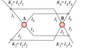
Figure 2.5: The left Kronecker product of two 4th-order tensors, $\underline{{\bf A}}$ and $\underline{{\bf B}}$, yields a 4th-order tensor, ${\underline{{\bf C}}}={\underline{{\bf A}}}\otimes_{L}{\underline{{\bf B}}}\in\mathbb{R}^{I_{1}J_{1}\times\cdots\times I_{4}J_{4}}$, with entries $c_{k_{1},k_{2},k_{3},k_{4}}=a_{i_{1},\ldots,i_{4}}\>b_{j_{1},\ldots,j_{4}}$, where $k_{n}=\overline{i_{n}j_{n}}$ ($n=1,2,3,4$). Note that the order of tensor $\underline{{\bf C}}$ is the same as the order of $\underline{{\bf A}}$ and $\underline{{\bf B}}$, but the size in every mode within $\underline{{\bf C}}$ is a product of the respective sizes of $\underline{{\bf A}}$ and $\underline{{\bf B}}$.

The Kronecker product of tensors. The (Left) Kronecker product of two $N$th-order tensors, $\underline{{\bf A}}\in\mathbb{R}^{I_{1}\times I_{2}\times\cdots\times I_{N}}$ and $\underline{{\bf B}}\in\mathbb{R}^{J_{1}\times J_{2}\times\cdots\times J_{N}}$, yields a tensor $\underline{{\bf C}}=\underline{{\bf A}}\otimes_{L}\underline{{\bf B}}\in\mathbb{R}^{I_{1}J_{1}\times\cdots\times I_{N}J_{N}}$ of the same order but enlarged in size, with entries $c_{\overline{i_{1}j_{1}},\ldots,\overline{i_{N}j_{N}}}=a_{i_{1},\ldots,i_{N}}\>b_{j_{1},\ldots,j_{N}}$ as illustrated in Figure 2.5.

The mode-$n$ Khatri–Rao product of tensors. The Mode-$n$ Khatri–Rao product of two $N$th-order tensors, $\underline{{\bf A}}\in\mathbb{R}^{I_{1}\times I_{2}\times\cdots\times I_{n}\times\cdots\times I_{N}}$ and $\underline{{\bf B}}\in\mathbb{R}^{J_{1}\times J_{2}\times\cdots\times J_{n}\times\cdots\times J_{N}}$, for which $I_{n}=J_{n}$, yields a tensor $\underline{{\bf C}}=\underline{{\bf A}}\odot_{\;n}\underline{{\bf B}}\in\mathbb{R}^{I_{1}J_{1}\times\cdots\times I_{n-1}J_{n-1}\times I_{n}\times I_{n+1}J_{n+1}\times\cdots\times I_{N}J_{N}}$, with subtensors $\underline{{\bf C}}(:,\ldots:,i_{n},:,\ldots,:)=\underline{{\bf A}}(:,\ldots:,i_{n},:,\ldots,:)\otimes\underline{{\bf B}}(:,\ldots:,i_{n},:,\ldots,:)$.

The mode-$2$ and mode-1 Khatri–Rao product of matrices. The above definition simplifies to the standard Khatri–Rao (mode-2) product of two matrices, ${\bf A}=[{\bf a}_{1},{\bf a}_{2},\ldots,{\bf a}_{R}]\in\mathbb{R}^{I\times R}$ and ${\bf B}=[{\bf b}_{1},{\bf b}_{2},\ldots,{\bf b}_{R}]\in\mathbb{R}^{J\times R}$, or in other words a “column-wise Kronecker product”. Therefore, the standard Right and Left Khatri–Rao products for matrices are respectively given by

$${\bf A}\odot{\bf B} = [{\bf a}_{1}\otimes{\bf b}_{1},{\bf a}_{2}\otimes{\bf b}_{2},\ldots,{\bf a}_{R}\otimes{\bf b}_{R}]\in\mathbb{R}^{IJ\times R},$$ (2.6)

$${\bf A}\odot_{L}{\bf B} = [{\bf a}_{1}\otimes_{L}{\bf b}_{1},{\bf a}_{2}\otimes_{L}{\bf b}_{2},\ldots,{\bf a}_{R}\otimes_{L}{\bf b}_{R}]\in\mathbb{R}^{IJ\times R}.$$ (2.7)

Analogously, the mode-1 Khatri–Rao product of two matrices ${\bf A}\in\mathbb{R}^{I\times R}$ and ${\bf B}\in\mathbb{R}^{I\times Q}$, is defined as

$${\bf A}\odot_{1}{\bf B}=\left[\begin{matrix}{\bf A}(1,:)\otimes{\bf B}(1,:)\\ \vdots\\ {\bf A}(I,:)\otimes{\bf B}(I,:)\end{matrix}\right]\in\mathbb{R}^{I\times RQ}.$$ (2.8)

Direct sum of tensors. A direct sum of $N$th-order tensors $\underline{{\bf A}}\in\mathbb{R}^{I_{1}\times\cdots\times I_{N}}$ and $\underline{{\bf B}}\in\mathbb{R}^{J_{1}\times\cdots\times J_{N}}$ yields a tensor $\underline{{\bf C}}=\underline{{\bf A}}\oplus\underline{{\bf B}}\in\mathbb{R}^{(I_{1}+J_{1})\times\cdots\times(I_{N}+J_{N})}$, with entries $\underline{{\bf C}}(k_{1},\ldots,k_{N})=\underline{{\bf A}}(k_{1},\ldots,k_{N})$ if $1\leq k_{n}\leq I_{n}$,   $\forall n$, $\underline{{\bf C}}(k_{1},\ldots,k_{N})=\underline{{\bf B}}(k_{1}-I_{1},\ldots,k_{N}-I_{N})$ if $I_{n}<k_{n}\leq I_{n}+J_{n}$,   $\forall n$, and $\underline{{\bf C}}(k_{1},\ldots,k_{N})=0$, otherwise (see Figure 2.6(a)).

Partial (mode-$n$) direct sum of tensors. A partial direct sum of tensors $\underline{{\bf A}}\in\mathbb{R}^{I_{1}\times\cdots\times I_{N}}$ and $\underline{{\bf B}}\in\mathbb{R}^{J_{1}\times\cdots\times J_{N}}$, with $I_{n}=J_{n}$, yields a tensor $\underline{{\bf C}}=\underline{{\bf A}}\oplus_{\;\overline{n}}\underline{{\bf B}}\in\mathbb{R}^{(I_{1}+J_{1})\times\cdots\times(I_{n-1}+J_{n-1})\times I_{n}\times(I_{n+1}+J_{n+1})\times\cdots\times(I_{N}+J_{N})}$, where $\underline{{\bf C}}(:,\ldots,:,i_{n},:,\ldots,:)=\underline{{\bf A}}(:,\ldots,:,i_{n},:,\ldots,:)\oplus\underline{{\bf B}}(:,\ldots,:,i_{n},:,\ldots,:)$, as illustrated in Figure 2.6(b).

Concatenation of $N$th-order tensors. A concatenation along mode-$n$ of tensors $\underline{{\bf A}}\in\mathbb{R}^{I_{1}\times\cdots\times I_{N}}$ and $\underline{{\bf B}}\in\mathbb{R}^{J_{1}\times\cdots\times J_{N}}$, for which $I_{m}=J_{m}$, $\;\forall m\neq n$ yields a tensor $\underline{{\bf C}}=\underline{{\bf A}}\boxplus_{\;n}\underline{{\bf B}}\in\mathbb{R}^{I_{1}\times\cdots\times I_{n-1}\times(I_{n}+J_{n})\times I_{n+1}\times\cdots\times(I_{N})}$, with subtensors $\underline{{\bf C}}(i_{1},\ldots,i_{n-1},:,i_{n+1},\ldots,i_{N})=\underline{{\bf A}}(i_{1},\ldots,i_{n-1},:,i_{n+1},\ldots,i_{N})\oplus\underline{{\bf B}}(i_{1},\ldots,i_{n-1},:,i_{n+1},\ldots,i_{N})$, as illustrated in Figure 2.6(c). For a concatenation of two tensors of suitable dimensions along mode-$n$, we will use equivalent notations $\underline{{\bf C}}=\underline{{\bf A}}\boxplus_{\;n}\underline{{\bf B}}=\underline{{\bf A}}\frown_{\;n}\underline{{\bf B}}$.

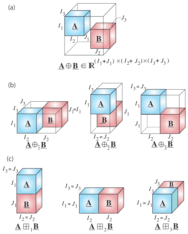
Figure 2.6: Illustration of the direct sum, partial direct sum and concatenation operators of two 3rd-order tensors. (a) Direct sum. (b) Partial (mode-1, mode-2, and mode-3) direct sum. (c) Concatenations along mode-1,2,3.

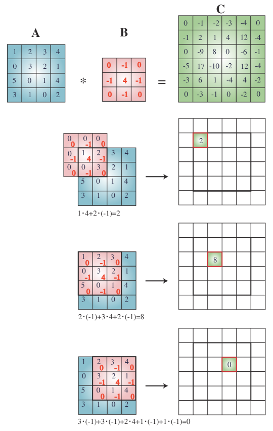
Figure 2.7: Illustration of the 2D convolution operator, performed through a sliding window operation along both the horizontal and vertical index.

3D Convolution. For simplicity, consider two 3rd-order tensors $\underline{{\bf A}}\in\mathbb{R}^{I_{1}\times I_{2}\times I_{3}}$ and $\underline{{\bf B}}\in\mathbb{R}^{J_{1}\times J_{2}\times J_{3}}$. Their 3D Convolution yields a tensor $\underline{{\bf C}}=\underline{{\bf A}}\ast\underline{{\bf B}}\in\mathbb{R}^{(I_{1}+J_{1}-1)\times(I_{2}+J_{2}-1)\times(I_{3}+J_{3}-1)}$, with entries:
$\underline{{\bf C}}(k_{1},k_{2},k_{3})=\sum_{j_{1}}\sum_{j_{2}}\sum_{j_{3}}\;\underline{{\bf B}}(j_{1},j_{2},j_{3})\;\underline{{\bf A}}(k_{1}-j_{1},k_{2}-j_{2},k_{3}-j_{3})$ as illustrated in Figure 2.7 and Figure 2.8.

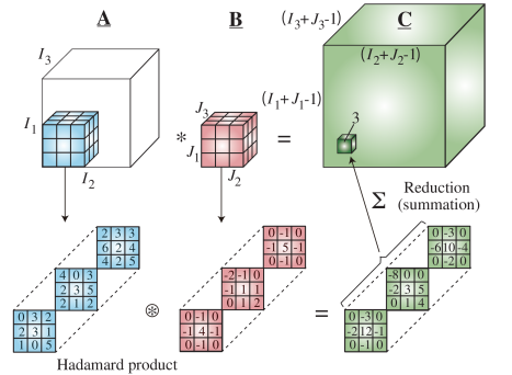
Figure 2.8: Illustration of the 3D convolution operator, performed through a sliding window operation along all three indices.

Partial (mode-$n$) Convolution. For simplicity, consider two 3rd-order tensors $\underline{{\bf A}}\in\mathbb{R}^{I_{1}\times I_{2}\times I_{3}}$ and $\underline{{\bf B}}\in\mathbb{R}^{J_{1}\times J_{2}\times J_{3}}$. Their mode-$2$ (partial) convolution yields a tensor $\underline{{\bf C}}=\underline{{\bf A}}\boxdot_{2}\underline{{\bf B}}\in\mathbb{R}^{I_{1}J_{1}\times(I_{2}+J_{2}-1)\times I_{3}J_{3}}$, the subtensors (vectors) of which are $\underline{{\bf C}}(k_{1},:,k_{3})=\underline{{\bf A}}(i_{1},:,i_{3})\ast\underline{{\bf B}}(j_{1},:,j_{3})\in\mathbb{R}^{I_{2}+J_{2}-1}$, where $k_{1}=\overline{i_{1}j_{1}}$, and $k_{3}=\overline{i_{3}j_{3}}$.

Outer product. The central operator in tensor analysis is the outer or tensor product, which for the tensors $\underline{{\bf A}}\in\mathbb{R}^{I_{1}\times\cdots\times I_{N}}$ and $\underline{{\bf B}}\in\mathbb{R}^{J_{1}\times\cdots\times J_{M}}$ gives the tensor $\underline{{\bf C}}=\underline{{\bf A}}\circ\underline{{\bf B}}\in\mathbb{R}^{I_{1}\times\cdots\times I_{N}\times J_{1}\times\cdots\times J_{M}}$ with entries $c_{i_{1},\ldots,i_{N},j_{1},\ldots,j_{M}}=a_{i_{1},\ldots,i_{N}}\;b_{j_{1},\ldots,j_{M}}$.

Note that for 1st-order tensors (vectors), the tensor product reduces to the standard outer product of two nonzero vectors, ${\bf a}\in\mathbb{R}^{I}$ and ${\bf b}\in\mathbb{R}^{J}$, which yields a rank-1 matrix, ${\bf X}={\bf a}\circ{\bf b}={\bf a}{\bf b}^{\text{T}}\in\mathbb{R}^{I\times J}$. The outer product of three nonzero vectors, ${\bf a}\in\mathbb{R}^{I},\;{\bf b}\in\mathbb{R}^{J}$ and ${\bf c}\in\mathbb{R}^{K}$, gives a 3rd-order rank-1 tensor (called pure or elementary tensor), $\underline{{\bf X}}={\bf a}\circ{\bf b}\circ{\bf c}\in\mathbb{R}^{I\times J\times K}$, with entries $x_{ijk}=a_{i}\;b_{j}\;c_{k}$.

Rank-1 tensor. A tensor, $\underline{{\bf X}}\in\mathbb{R}^{I_{1}\times I_{2}\times\cdots\times I_{N}}$, is said to be of rank-1 if it can be expressed exactly as the outer product, $\underline{{\bf X}}={\bf b}^{(1)}\circ{\bf b}^{(2)}\circ\cdots\circ{\bf b}^{(N)}$ of nonzero vectors, ${\bf b}^{(n)}\in\mathbb{R}^{I_{n}}$, with the tensor entries given by $x_{i_{1},i_{2},\ldots,i_{N}}=b^{(1)}_{i_{1}}b^{(2)}_{i_{2}}\cdots b^{(N)}_{i_{N}}$.

Kruskal tensor, CP decomposition. For further discussion, it is important to highlight that any tensor can be expressed as a finite sum of rank-1 tensors, in the form

$$\underline{{\bf X}}=\sum_{r=1}^{R}{\bf b}_{r}^{(1)}\circ{\bf b}_{r}^{(2)}\circ\cdots\circ{\bf b}_{r}^{(N)}=\sum_{r=1}^{R}\;\left(\overset{N}{\underset{n=1}{\circ}}\;{\bf b}_{r}^{(n)}\right),\ \ {\bf b}_{r}^{(n)}\in\mathbb{R}^{I_{n}},$$ (2.9)

which is exactly the form of the Kruskal tensor, illustrated in Figure 2.9, also known under the names of CANDECOMP / PARAFAC, Canonical Polyadic Decomposition (CPD), or simply the CP decomposition in (1.2). We will use the acronyms CP and CPD.

Tensor rank. The tensor rank, also called the CP rank, is a natural extension of the matrix rank and is defined as a minimum number, $R$, of rank-1 terms in an exact CP decomposition of the form in (2.9).

Although the CP decomposition has already found many practical applications, its limiting theoretical property is that the best rank-$R$ approximation of a given data tensor may not exist (see [63] for more detail). However, a rank-$R$ tensor can be approximated arbitrarily well by a sequence of tensors for which the CP ranks are strictly less than $R$. For these reasons, the concept of border rank was proposed [21], which is defined as the minimum number of rank-1 tensors which provides the approximation of a given tensor with an arbitrary accuracy.

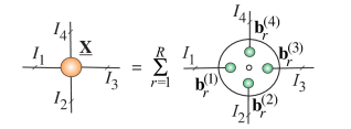
Figure 2.9: The CP decomposition for a 4th-order tensor $\underline{{\bf X}}$ of rank $R$. Observe that the rank-1 subtensors are formed through the outer products of the vectors ${\bf b}_{r}^{(1)},\ldots,{\bf b}_{r}^{(4)}$, $r=1,\ldots,R$.

Symmetric tensor decomposition. A symmetric tensor (sometimes called a super-symmetric tensor) is invariant to the permutations of its indices. A symmetric tensor of $N$th-order has equal sizes, $I_{n}=I,\,\forall n$, in all its modes, and the same value of entries for every permutation of its indices. For example, for vectors ${\bf b}^{(n)}={\bf b}\in\mathbb{R}^{I},\;\forall n$, the rank-1 tensor, constructed by $N$ outer products, $\circ_{n=1}^{N}{\bf b}^{(n)}={\bf b}\circ{\bf b}\circ\cdots\circ{\bf b}\in\mathbb{R}^{I\times I\times\cdots\times I}$, is symmetric. Moreover, every symmetric tensor can be expressed as a linear combination of such symmetric rank-1 tensors through the so-called symmetric CP decomposition, given by

$$\underline{{\bf X}}=\sum_{r=1}^{R}\lambda_{r}{\bf b}_{r}\circ{\bf b}_{r}\circ\cdots\circ{\bf b}_{r},\qquad{\bf b}_{r}\in\mathbb{R}^{I},$$ (2.10)

where $\lambda_{r}\in\mathbb{R}$ are the scaling parameters for the unit length vectors ${\bf b}_{r}$, while the symmetric tensor rank is the minimal number $R$ of rank-1 tensors that is necessary for its exact representation.

(a)

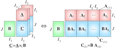
(b)

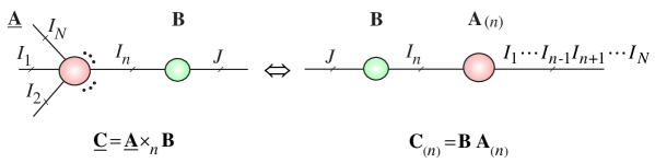
Figure 2.10: Illustration of the multilinear mode-$n$ product, also known as the TTM (Tensor-Times-Matrix) product, performed in the tensor format (left) and the matrix format (right). (a) Mode-$1$ product of a 3rd-order tensor, $\underline{{\bf A}}\in\mathbb{R}^{I_{1}\times I_{2}\times I_{3}}$, and a factor (component) matrix, ${\bf B}\in\mathbb{R}^{J\times I_{1}}$, yields a tensor $\underline{{\bf C}}=\underline{{\bf A}}\times_{1}{\bf B}\in\mathbb{R}^{J\times I_{2}\times I_{3}}$. This is equivalent to a simple matrix multiplication formula, ${\bf C}_{(1)}={\bf B}{\bf A}_{(1)}$. (b) Graphical representation of a mode-$n$ product of an $N$th-order tensor, $\underline{{\bf A}}\in\mathbb{R}^{I_{1}\times I_{2}\times\cdots\times I_{N}}$, and a factor matrix, ${\bf B}\in\mathbb{R}^{J\times I_{n}}$.

Multilinear products. The mode-$n$ (multilinear) product, also called the tensor-times-matrix product (TTM), of a tensor, $\underline{{\bf A}}\in\mathbb{R}^{I_{1}\times\cdots\times I_{N}}$, and a matrix, ${\bf B}\in\mathbb{R}^{J\times I_{n}}$, gives the tensor

$$\underline{{\bf C}}=\underline{{\bf A}}\times_{n}{\bf B}\in\mathbb{R}^{I_{1}\times\cdots\times I_{n-1}\times J\times I_{n+1}\times\cdots\times I_{N}},$$ (2.11)

with entries

$$c_{i_{1},i_{2},\ldots,i_{n-1},j,i_{n+1},\ldots,i_{N}}=\sum_{i_{n}=1}^{I_{n}}a_{i_{1},i_{2},\ldots,i_{N}}\;b_{j,i_{n}}.$$ (2.12)

From (2.12) and Figure 2.10, the equivalent matrix form is ${\bf C}_{(n)}={\bf B}{\bf A}_{(n)}$, which allows us to employ established fast matrix-by-vector and matrix-by-matrix multiplications when dealing with very large-scale tensors. Efficient and optimized algorithms for TTM are, however, still emerging [131, 11, 12].

Full multilinear (Tucker) product. A full multilinear product, also called the Tucker product, of an $N$th-order tensor, $\underline{{\bf G}}\in\mathbb{R}^{R_{1}\times R_{2}\times\cdots\times R_{N}}$, and a set of $N$ factor matrices, $\underline{{\bf B}}^{(n)}\in\mathbb{R}^{I_{n}\times R_{n}}$ for $n=1,2,\ldots,N$, performs the multiplications in all the modes and can be compactly written as (see Figure 2.11(b))

$$\underline{{\bf C}} = \underline{{\bf G}}\times_{1}{\bf B}^{(1)}\times_{2}{\bf B}^{(2)}\cdots\times_{N}{\bf B}^{(N)}$$

$$= \llbracket\underline{{\bf G}};{\bf B}^{(1)},{\bf B}^{(2)},\ldots,{\bf B}^{(N)}\rrbracket\in\mathbb{R}^{I_{1}\times I_{2}\times\cdots\times I_{N}}.$$

Observe that this format corresponds to the Tucker decomposition [210, 209, 119] (see Section 3.3).

Multilinear product of a tensor and a vector (TTV). In a similar way, the mode-$n$ multiplication of a tensor, $\underline{{\bf A}}\in\mathbb{R}^{I_{1}\times\cdots\times I_{N}}$, and a vector, ${\bf b}\in\mathbb{R}^{I_{n}}$ (tensor-times-vector, TTV) yields a tensor

$$\underline{{\bf C}}=\underline{{\bf A}}\bar{\times}_{n}{\bf b}\in\mathbb{R}^{I_{1}\times\cdots\times I_{n-1}\times I_{n+1}\times\cdots\times I_{N}},$$ (2.14)

with entries

$$c_{i_{1},\ldots,i_{n-1},i_{n+1},\ldots,i_{N}}=\sum_{i_{n}=1}^{I_{n}}a_{i_{1},\ldots,i_{n-1},i_{n},i_{n+1},\ldots,i_{N}}\;b_{i_{n}}.$$ (2.15)

Note that the mode-$n$ multiplication of a tensor by a matrix does not change the tensor order, while the multiplication of a tensor by vectors reduces its order, with the mode $n$ removed (see Figure 2.11).

(a)

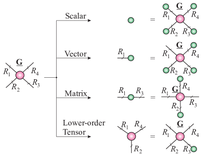
(b)                                                     (c)

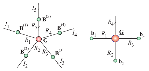
Figure 2.11: Multilinear tensor products in a compact tensor network notation. (a) Transforming and/or compressing a 4th-order tensor, $\underline{{\bf G}}\in\mathbb{R}^{R_{1}\times R_{2}\times R_{3}\times R_{4}}$, into a scalar, vector, matrix and 3rd-order tensor, by multilinear products of the tensor and vectors. Note that a mode-$n$ multiplication of a tensor by a matrix does not change the order of a tensor, while a multiplication of a tensor by a vector reduces its order by one. For example, a multilinear product of a 4th-order tensor and four vectors (top diagram) yields a scalar. (b) Multilinear product of a tensor, $\underline{{\bf G}}\in\mathbb{R}^{R_{1}\times R_{2}\times\cdots\times R_{5}}$, and five factor (component) matrices, ${\bf B}^{(n)}\in\mathbb{R}^{I_{n}\times R_{n}}$ ($n=1,2,\ldots,5$), yields the tensor $\underline{{\bf C}}=\underline{{\bf G}}\times_{1}{\bf B}^{(1)}\times_{2}{\bf B}^{(2)}\times_{3}{\bf B}^{(3)}\times_{4}{\bf B}^{(4)}\times_{5}{\bf B}^{(5)}\in\mathbb{R}^{I_{1}\times I_{2}\times\cdots\times I_{5}}$. This corresponds to the Tucker format. (c) Multilinear product of a 4th-order tensor, $\underline{{\bf G}}\in\mathbb{R}^{R_{1}\times R_{2}\times R_{3}\times R_{4}}$, and three vectors, ${\bf b}_{n}\in\mathbb{R}^{R_{n}}$ $(n=1,2,3)$, yields the vector ${\bf c}=\underline{{\bf G}}\bar{\times}_{1}{\bf b}_{1}\bar{\times}_{2}{\bf b}_{2}\bar{\times}_{3}{\bf b}_{3}\in\mathbb{R}^{R_{4}}$.

Multilinear products of tensors by matrices or vectors play a key role in deterministic methods for the reshaping of tensors and dimensionality reduction, as well as in probabilistic methods for randomization / sketching procedures and in random projections of tensors into matrices or vectors. In other words, we can also perform reshaping of a tensor through random projections that change its entries, dimensionality or size of modes, and/or the tensor order. This is achieved by multiplying a tensor by random matrices or vectors, transformations which preserve its basic properties. [199, 72, 137, 132, 168, 223, 126, 192] (see Section 3.5 for more detail).

Tensor contractions. Tensor contraction is a fundamental and the most important operation in tensor networks, and can be considered a higher-dimensional analogue of matrix multiplication, inner product, and outer product.

In a way similar to the mode-$n$ multilinear product, the mode-$(_{n}^{m})$ product (tensor contraction) of two tensors, $\underline{{\bf A}}\in\mathbb{R}^{I_{1}\times I_{2}\times\cdots\times I_{N}}$ and $\underline{{\bf B}}\in\mathbb{R}^{J_{1}\times J_{2}\times\cdots\times J_{M}}$, with common modes, $I_{n}=J_{m}$, yields an $(N+M-2)$-order tensor, $\underline{{\bf C}}\in\mathbb{R}^{I_{1}\times\cdots\times I_{n-1}\times I_{n+1}\times\cdots\times I_{N}\times J_{1}\times\cdots\times J_{m-1}\times J_{m+1}\times\cdots\times J_{M}}$, in the form (see Figure 2.12(a))

$$\underline{{\bf C}}=\underline{{\bf A}}\;{\times}_{n}^{m}\;\underline{{\bf B}},$$ (2.16)

for which the entries are computed as

$$c_{i_{1},\,\ldots,\,i_{n-1},\,i_{n+1},\,\ldots,i_{N},\,j_{1},\,\ldots,\,j_{m-1},\,j_{m+1},\,\ldots,\,j_{M}}=$$

$$=\sum_{i_{n}=1}^{I_{n}}a_{i_{1},\ldots,i_{n-1},\,i_{n},\,i_{n+1},\,\ldots,\,i_{N}}\;b_{j_{1},\,\ldots,\,j_{m-1},\,i_{n},\,j_{m+1},\,\ldots,\,j_{M}}.$$ (2.17)

This operation is referred to as a contraction of two tensors in single common mode.

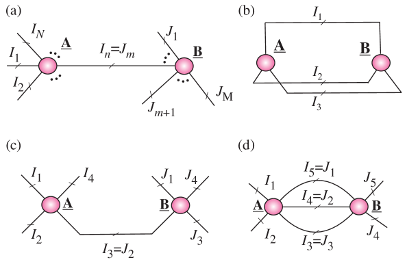
Figure 2.12: Examples of contractions of two tensors. (a) Multilinear product of two tensors is denoted by $\underline{{\bf A}}\;\times_{n}^{m}\;\underline{{\bf B}}$. (b) Inner product of two 3rd-order tensors yields a scalar $c=\langle\underline{{\bf A}},\underline{{\bf B}}\rangle=\underline{{\bf A}}\;\times_{1,2,3}^{1,2,3}\;\underline{{\bf B}}=\underline{{\bf A}}\;\bar{\times}\;\underline{{\bf B}}=\sum_{i_{1},i_{2},i_{3}}\;a_{i_{1},i_{2},i_{3}}\;b_{i_{1},i_{2},i_{3}}$. (c) Tensor contraction of two 4th-order tensors, along mode-3 in $\underline{{\bf A}}$ and mode-2 in $\underline{{\bf B}}$, yields a 6th-order tensor, $\underline{{\bf C}}=\underline{{\bf A}}\;\times_{3}^{2}\;\underline{{\bf B}}\in\mathbb{R}^{I_{1}\times I_{2}\times I_{4}\times J_{1}\times J_{3}\times J_{4}}$, with entries $c_{i_{1},i_{2},i_{4},j_{1},j_{3},j_{4}}=\sum_{i_{3}}\;a_{i_{1},i_{2},i_{3},i_{4}}\;b_{j_{1},i_{3},j_{3},j_{4}}$. (d) Tensor contraction of two 5th-order tensors along the modes $3,4,5$ in $\underline{{\bf A}}$ and $1,2,3$ in $\underline{{\bf B}}$ yields a 4th-order tensor, $\underline{{\bf C}}=\underline{{\bf A}}\;\times_{5,4,3}^{1,2,3}\;\underline{{\bf B}}\in\mathbb{R}^{I_{1}\times I_{2}\times J_{4}\times J_{5}}$.

Tensors can be contracted in several modes or even in all modes, as illustrated in Figure 2.12. For convenience of presentation, the super- or sub-index, e.g., $m,n$, will be omitted in a few special cases. For example, the multilinear product of the tensors, $\underline{{\bf A}}\in\mathbb{R}^{I_{1}\times I_{2}\times\cdots\times I_{N}}$ and $\underline{{\bf B}}\in\mathbb{R}^{J_{1}\times J_{2}\times\cdots\times J_{M}}$, with common modes, $I_{N}=J_{1}$, can be written as

$$\underline{{\bf C}}=\underline{{\bf A}}\;\times_{N}^{1}\;\underline{{\bf B}}=\underline{{\bf A}}\times^{1}\underline{{\bf B}}=\underline{{\bf A}}\bullet\underline{{\bf B}}\in\mathbb{R}^{I_{1}\times I_{2}\times\cdots\times I_{N-1}\times J_{2}\times\cdots\times J_{M}},$$ (2.18)

for which the entries

$$c_{i_{1},i_{2},\ldots,i_{N-1},j_{2},j_{3},\ldots,j_{M}}=\sum_{i_{N}=1}^{I_{N}}a_{i_{1},i_{2},\ldots,i_{N}}\;b_{i_{N},j_{2},\ldots,j_{M}}.$$

In this notation, the multiplications of matrices and vectors can be written as, ${\bf A}\times^{1}_{2}{\bf B}={\bf A}\times^{1}{\bf B}={\bf A}{\bf B}$, $\;{\bf A}\times^{2}_{2}{\bf B}={\bf A}{\bf B}^{\text{T}}$, $\;{\bf A}\times^{1,2}_{1,2}\;{\bf B}={\bf A}\bar{\times}{\bf B}=\langle{\bf A},{\bf B}\rangle$, and ${\bf A}\times^{1}_{2}\;{\bf x}={\bf A}\times^{1}{\bf x}={\bf A}{\bf x}$.

Note that tensor contractions are, in general not associative or commutative, since when contracting more than two tensors, the order has to be precisely specified (defined), for example, $\underline{{\bf A}}\times^{b}_{a}(\underline{{\bf B}}\times_{c}^{d}\underline{{\bf C}})$ for $b<c$.

It is also important to note that a matrix-by-vector product, ${\bf y}={\bf A}{\bf x}\in\mathbb{R}^{I_{1}\cdots I_{N}}$, with ${\bf A}\in\mathbb{R}^{I_{1}\cdots I_{N}\times J_{1}\cdots J_{N}}$ and ${\bf x}\in\mathbb{R}^{J_{1}\cdots J_{N}}$, can be expressed in a tensorized form via the contraction operator as $\underline{{\bf Y}}=\underline{{\bf A}}\bar{\times}\underline{{\bf X}}$, where the symbol $\bar{\times}$ denotes the contraction of all modes of the tensor $\underline{{\bf X}}$ (see Section 4.5).

Unlike the matrix-by-matrix multiplications for which several efficient parallel schemes have been developed, (e.g. BLAS procedure) the number of efficient algorithms for tensor contractions is rather limited. In practice, due to the high computational complexity of tensor contractions, especially for tensor networks with loops, this operation is often performed approximately [138, 66, 167, 107].

Tensor trace. Consider a tensor with partial self-contraction modes, where the outer (or open) indices represent physical modes of the tensor, while the inner indices indicate its contraction modes. The Tensor Trace operator performs the summation of all inner indices of the tensor [89]. For example, a tensor $\underline{{\bf A}}$ of size $R\times I\times R$ has two inner indices, modes 1 and 3 of size $R$, and one open mode of size $I$. Its tensor trace yields a vector of length $I$, given by

$${\bf a}=\mbox{Tr}(\underline{{\bf A}})=\sum_{r}\underline{{\bf A}}(r,:,r)\,,$$

the elements of which are the traces of its lateral slices ${\bf A}_{i}\in\mathbb{R}^{R\times R}$ $\;(i=1,2,\ldots,I)$, that is, (see bottom of Figure 2.13)

$${\bf a}=[\mathop{\rm tr}\nolimits({\bf A}_{1}),\ldots,\mathop{\rm tr}\nolimits({\bf A}_{i}),\ldots,\mathop{\rm tr}\nolimits({\bf A}_{I})]^{\text{T}}.$$ (2.19)

A tensor can have more than one pair of inner indices, e.g., the tensor $\underline{{\bf A}}$ of size $R\times I\times S\times S\times I\times R$ has two pairs of inner indices, modes 1 and 6, modes 3 and 4, and two open modes (2 and 5). The tensor trace of $\underline{{\bf A}}$ therefore returns a matrix of size $I\times I$ defined as

$$\mbox{Tr}(\underline{{\bf A}})=\sum_{r}\sum_{s}\underline{{\bf A}}(r,:,s,s,:,r)\,.$$

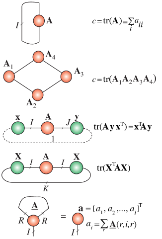
Figure 2.13: Tensor network notation for the traces of matrices (panels 1-4 from the top), and a (partial) tensor trace (tensor self-contraction) of a 3rd-order tensor (bottom panel). Note that graphical representations of the trace of matrices intuitively explain the permutation property of trace operator, e.g., $\mathop{\rm tr}\nolimits({\bf A}_{1}{\bf A}_{2}{\bf A}_{3}{\bf A}_{4})=\mathop{\rm tr}\nolimits({\bf A}_{3}{\bf A}_{4}{\bf A}_{1}{\bf A}_{2})$.

A variant of Tensor Trace [128] for the case of the partial tensor self-contraction considers a tensor $\underline{{\bf A}}\in\mathbb{R}^{R\times I_{1}\times I_{2}\times\cdots\times I_{N}\times R}$ and yields a reduced-order tensor $\underline{\widetilde{\bf A}}=\mbox{Tr}(\underline{{\bf A}})\in\mathbb{R}^{I_{1}\times I_{2}\times\cdots\times I_{N}}$, with entries

$$\underline{\widetilde{\bf A}}(i_{1},i_{2},\ldots,i_{N})=\sum_{r=1}^{R}\underline{{\bf A}}(r,i_{1},i_{2},\ldots,i_{N},r),$$ (2.20)

Conversions of tensors to scalars, vectors, matrices or tensors with reshaped modes and/or reduced orders are illustrated in Figures 2.11– 2.13.

2.2 Graphical Representation of Fundamental Tensor Networks

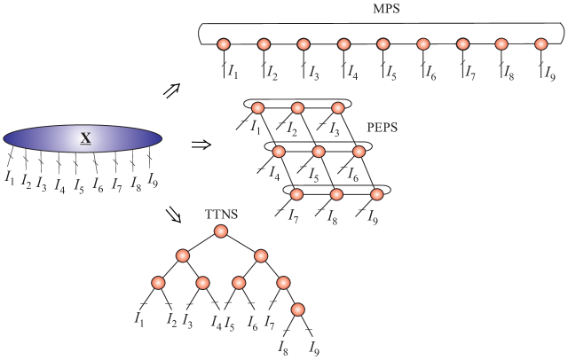
Figure 2.14: Illustration of the decomposition of a 9th-order tensor, $\underline{{\bf X}}\in\mathbb{R}^{I_{1}\times I_{2}\times\cdots\times I_{9}}$, into different forms of tensor networks (TNs). In general, the objective is to decompose a very high-order tensor into sparsely (weakly) connected low-order and small size tensors, typically 3rd-order and 4th-order tensors called cores. Top: The Tensor Chain (TC) model, which is equivalent to the Matrix Product State (MPS) with periodic boundary conditions (PBC). Middle: The Projected Entangled-Pair States (PEPS), also with PBC. Bottom: The Tree Tensor Network State (TTNS).

Tensor networks (TNs) represent a higher-order tensor as a set of sparsely interconnected lower-order tensors (see Figure 2.14), and in this way provide computational and storage benefits. The lines (branches, edges) connecting core tensors correspond to the contracted modes while their weights (or numbers of branches) represent the rank of a tensor network, whereas the lines which do not connect core tensors correspond to the “external” physical variables (modes, indices) within the data tensor. In other words, the number of free (dangling) edges (with weights larger than one) determines the order of a data tensor under consideration, while set of weights of internal branches represents the TN rank.

2.3 Hierarchical Tucker (HT) and Tree Tensor Network State (TTNS) Models

Hierarchical Tucker (HT) decompositions (also called hierarchical tensor representation) have been introduced in [92] and also independently in [86], see also [91, 139, 211, 122, 7] and references therein. Generally, the HT decomposition requires splitting the set of modes of a tensor in a hierarchical way, which results in a binary tree containing a subset of modes at each branch (called a dimension tree); examples of binary trees are given in Figures 2.15, 2.16 and 2.17. In tensor networks based on binary trees, all the cores are of order of three or less. Observe that the HT model does not contain any cycles (loops), i.e., no edges connecting a node with itself. The splitting operation of the set of modes of the original data tensor by binary tree edges is performed through a suitable matricization.

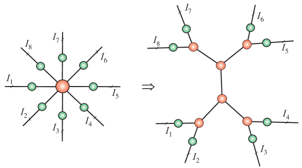
Figure 2.15: The standard Tucker decomposition of an 8th-order tensor into a core tensor (red circle) and eight factor matrices (green circles), and its transformation into an equivalent Hierarchical Tucker (HT) model using interconnected smaller size 3rd-order core tensors and the same factor matrices.

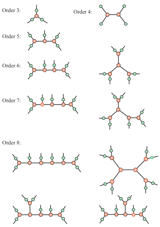
Figure 2.16: Examples of HT/TT models (formats) for distributed Tucker decompositions with 3rd-order cores, for different orders of data tensors. Green circles denote factor matrices (which can be absorbed by core tensors), while red circles indicate cores. Observe that the representations are not unique.

Choice of dimension tree. The dimension tree within the HT format is chosen a priori and defines the topology of the HT decomposition. Intuitively, the dimension tree specifies which groups of modes are “separated” from other groups of modes, so that a sequential HT decomposition can be performed via a (truncated) SVD applied to a suitably matricized tensor. One of the simplest and most straightforward choices of a dimension tree is the linear and unbalanced tree, which gives rise to the tensor-train (TT) decomposition, discussed in detail in Section 2.4 and Section 4 [158, 161].

Using mathematical formalism, a dimension tree is a binary tree $T_{N}$, $N>1$, which satisfies that

1. all nodes $t\in T_{N}$ are non-empty subsets of {1, 2,…, N},

2. the set $t_{root}=\{1,2,\ldots,N\}$ is the root node of $T_{N}$, and

3. each non-leaf node has two children $u,v\in T_{N}$ such that $t$ is a disjoint union $t=u\cup v$.

The HT model is illustrated through the following Example.
Example. Suppose that the dimension tree $T_{7}$ is given, which gives the HT decomposition illustrated in Figure 2.17. The HT decomposition of a tensor $\underline{{\bf X}}\in\mathbb{R}^{I_{1}\times\cdots\times I_{7}}$ with given set of integers $\{R_{t}\}_{t\in T_{7}}$ can be expressed in the tensor and vector / matrix forms as follows. Let intermediate tensors $\underline{{\bf X}}^{(t)}$ with $t=\{n_{1},\ldots,n_{k}\}\subset\{1,\ldots,7\}$ have the size $I_{n_{1}}\times I_{n_{2}}\times\cdots\times I_{n_{k}}\times R_{t}$. Let $\underline{{\bf X}}^{(t)}_{r_{t}}\equiv\underline{{\bf X}}^{(t)}(:,\ldots,:,r_{t})$ denote the subtensor of $\underline{{\bf X}}^{(t)}$ and ${\bf X}^{(t)}\equiv{\bf X}^{(t)}_{<k>}\in\mathbb{R}^{I_{n_{1}}I_{n_{2}}\cdots I_{n_{k}}\times R_{t}}$ denote the corresponding unfolded matrix. Let $\underline{{\bf G}}^{(t)}\in\mathbb{R}^{R_{u}\times R_{v}\times R_{t}}$ be core tensors where $u$ and $v$ denote respectively the left and right children of $t$.

The HT model shown in Figure 2.17 can be then described mathematically in the vector form as

$$\text{vec}(\underline{{\bf X}})\cong({\bf X}^{(123)}\otimes_{L}{\bf X}^{(4567)})\;\text{vec}({\bf G}^{(12\cdots 7)}),$$

$${\bf X}^{(123)}\cong({\bf B}^{(1)}\otimes_{L}{\bf X}^{(23)})\;{\bf G}^{(123)}_{<2>},\quad{\bf X}^{(4567)}\cong({\bf X}^{(45)}\otimes_{L}{\bf X}^{(67)})\;{\bf G}^{(4567)}_{<2>},$$

$${\bf X}^{(23)}\cong({\bf B}^{(2)}\otimes_{L}{\bf B}^{(3)})\;{\bf G}^{(23)}_{<2>},\qquad{\bf X}^{(45)}\cong({\bf B}^{(4)}\otimes_{L}{\bf B}^{(5)})\;{\bf G}^{(45)}_{<2>},$$

$${\bf X}^{(67)}\cong({\bf B}^{(6)}\otimes_{L}{\bf B}^{(7)})\;{\bf G}^{(67)}_{<2>}.$$

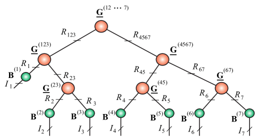
Figure 2.17: Example illustrating the HT decomposition for a 7th-order data tensor.

An equivalent, more explicit form, using tensor notations becomes

$$\underline{{\bf X}}\cong\sum_{r_{123}=1}^{R_{123}}\sum_{r_{4567}=1}^{R_{4567}}g^{(12\cdots 7)}_{r_{123},r_{4567}}\;{\underline{{\bf X}}}^{(123)}_{r_{123}}\circ{\underline{{\bf X}}}^{(4567)}_{r_{4567}},$$

$${\underline{{\bf X}}}^{(123)}_{r_{123}}\cong\sum_{r_{1}=1}^{R_{1}}\sum_{r_{23}=1}^{R_{23}}g^{(123)}_{r_{1},r_{23},r_{123}}{{\bf b}}^{(1)}_{r_{1}}\circ{{\bf X}}^{(23)}_{r_{23}},$$

$${\underline{{\bf X}}}^{(4567)}_{r_{4567}}\cong\sum_{r_{45}=1}^{R_{45}}\sum_{r_{67}=1}^{R_{67}}g^{(4567)}_{r_{45},r_{67},r_{4567}}{{\bf X}}^{(45)}_{r_{45}}\circ{{\bf X}}^{(67)}_{r_{67}},$$

$${{\bf X}}^{(23)}_{r_{23}}\cong\sum_{r_{2}=1}^{R_{2}}\sum_{r_{3}=1}^{R_{3}}g^{(23)}_{r_{2},r_{3},r_{23}}\;{{\bf b}}^{(2)}_{r_{2}}\circ{{\bf b}}^{(3)}_{r_{3}},$$

$${{\bf X}}^{(45)}_{r_{45}}\cong\sum_{r_{4}=1}^{R_{4}}\sum_{r_{5}=1}^{R_{5}}g^{(45)}_{r_{4},r_{5},r_{45}}\;{{\bf b}}^{(4)}_{r_{4}}\circ{{\bf b}}^{(5)}_{r_{5}},$$

$${{\bf X}}^{(67)}_{r_{67}}\cong\sum_{r_{6}=1}^{R_{6}}\sum_{r_{7}=1}^{R_{7}}g^{(67)}_{r_{6},r_{7},r_{67}}\;{{\bf b}}^{(6)}_{r_{6}}\circ{{\bf b}}^{(7)}_{r_{7}}.$$

The TT/HT decompositions lead naturally to a distributed Tucker decomposition, where a single core tensor is replaced by interconnected cores of lower-order, resulting in a distributed network in which only some cores are connected directly with factor matrices, as illustrated in Figure 2.15. Figure 2.16 illustrates exemplary HT/TT structures for data tensors of various orders [205, 122]. Note that for a 3rd-order tensor, there is only one HT tensor network representation, while for a 5th-order we have 5, and for a 10th-order tensor there are 11 possible HT architectures.

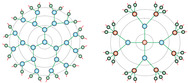
Figure 2.18: The Tree Tensor Network State (TTNS) with 3rd-order and 4th-order cores for the representation of 24th-order data tensors. The TTNS can be considered both as a generalization of HT/TT format and as a distributed model for the Tucker-$N$ decomposition (see Section 3.3).

A simple approach to reduce the size of a large-scale core tensor in the standard Tucker decomposition (typically, for $N>5$) would be to apply the concept of distributed tensor networks (DTNs). The DTNs assume two kinds of cores (blocks): (i) the internal cores (nodes) which are connected only to other cores and have no free edges and (ii) external cores which do have free edges representing physical modes (indices) of a given data tensor (see also Section 2.6). Such distributed representations of tensors are not unique.

The tree tensor network state (TTNS) model, whereby all nodes are of 3rd-order or higher, can be considered as a generalization of the TT/HT decompositions, as illustrated by two examples in Figure 2.18 [149]. A more detailed mathematical description of the TTNS is given in Section 3.3.

(a)

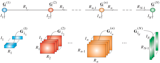
(b)

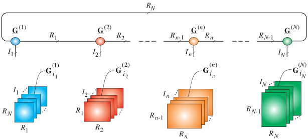
Figure 2.19: Concepts of the tensor train (TT) and tensor chain (TC) decompositions (MPS with OBC and PBC, respectively) for an $N$th-order data tensor, $\underline{{\bf X}}\in\mathbb{R}^{I_{1}\times I_{2}\times\cdots\times I_{N}}$. (a) Tensor Train (TT) can be mathematically described as $x_{i_{1},i_{2},\ldots,i_{N}}={\bf G}^{(1)}_{i_{1}}\;{\bf G}^{(2)}_{i_{2}}\;\cdots\;{\bf G}^{(N)}_{i_{N}}$, where (bottom panel) the slice matrices of TT-cores $\underline{{\bf G}}^{(n)}\in\mathbb{R}^{R_{n-1}\times I_{n}\times R_{n}}$ are defined as ${\bf G}^{(n)}_{i_{n}}=\underline{{\bf G}}^{(n)}(:,i_{n},:)\allowbreak\in\mathbb{R}^{R_{n-1}\times R_{n}}$ with $R_{0}=R_{N}=1$. (b) For the Tensor Chain (TC), the entries of a tensor are expressed as $x_{i_{1},i_{2},\ldots,i_{N}}=\mathop{\rm tr}\nolimits\,({\bf G}^{(1)}_{i_{1}}\;{\bf G}^{(2)}_{i_{2}}\;\cdots\;{\bf G}^{(N)}_{i_{N}})=\displaystyle\sum_{r_{1}=1}^{R_{1}}\sum_{r_{2}=1}^{R_{2}}\cdots\sum_{r_{N}=1}^{R_{N}}g^{(1)}_{\;r_{N},\,i_{1},\,r_{1}}\;g^{(2)}_{\;r_{1},\,i_{2},\,r_{2}}\cdots g^{(N)}_{\;r_{N-1},\,i_{N},\,r_{N}}$, where (bottom panel) the lateral slices of the TC-cores are defined as ${\bf G}^{(n)}_{i_{n}}=\underline{{\bf G}}^{(n)}(:,\,i_{n},\,:)\in\mathbb{R}^{R_{n-1}\times R_{n}}$ and $g^{(n)}_{\;r_{n-1},\,i_{n},\,r_{n}}=\underline{{\bf G}}^{(n)}(r_{n-1},\,i_{n},\,r_{n})$ for $n=1,2,\ldots,N$, with $R_{0}=R_{N}>1$. Notice that TC/MPS is effectively a TT with a single loop connecting the first and the last core, so that all TC-cores are of 3rd-order.

2.4 Tensor Train (TT) Network

The Tensor Train (TT) format can be interpreted as a special case of the HT format, where all nodes (TT-cores) of the underlying tensor network are connected in cascade (or train), i.e., they are aligned while factor matrices corresponding to the leaf modes are assumed to be identities and thus need not be stored. The TT format was first proposed in numerical analysis and scientific computing in [158, 161]. Figure 2.19 presents the concept of TT decomposition for an $N$th-order tensor, the entries of which can be computed as a cascaded (multilayer) multiplication of appropriate matrices (slices of TT-cores). The weights of internal edges (denoted by $\{R_{1},R_{2},\ldots,R_{N-1}\}$) represent the TT-rank. In this way, the so aligned sequence of core tensors represents a “tensor train” where the role of “buffers” is played by TT-core connections. It is important to highlight that TT networks can be applied not only for the approximation of tensorized vectors but also for scalar multivariate functions, matrices, and even large-scale low-order tensors, as illustrated in Figure 2.20 (for more detail see Section 4).

In the quantum physics community, the TT format is known as the Matrix Product State (MPS) representation with the Open Boundary Conditions (OBC) and was introduced in 1987 as the ground state of the 1D AKLT model [2]. It was subsequently extended by many researchers (see [224, 216, 166, 214, 183, 102, 156] and references therein).

Advantages of TT formats. An important advantage of the TT/MPS format over the HT format is its simpler practical implementation, as no binary tree needs to be determined (see Section 4). Another attractive property of the TT-decomposition is its simplicity when performing basic mathematical operations on tensors directly in the TT-format (that is, employing only core tensors). These include matrix-by-matrix and matrix-by-vector multiplications, tensor addition, and the entry-wise (Hadamard) product of tensors. These operations produce tensors, also in the TT-format, which generally exhibit increased TT-ranks. A detailed description of basic operations supported by the TT format is given in Section 4.5. Moreover, only TT-cores need to be stored and processed, which makes the number of parameters to scale linearly in the tensor order, $N$, of a data tensor and all mathematical operations are then performed only on the low-order and relatively small size core tensors.

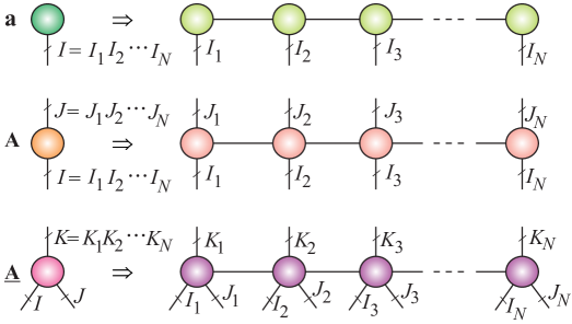
Figure 2.20: Forms of tensor train decompositions for a vector, ${\bf a}\in\mathbb{R}^{I}$, matrix, ${\bf A}\in\mathbb{R}^{I\times J}$, and 3rd-order tensor, $\underline{{\bf A}}\in\mathbb{R}^{I\times J\times K}$ (by applying a suitable tensorization).

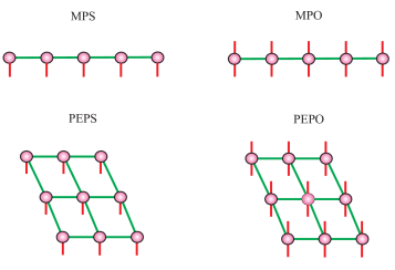
Figure 2.21: Class of 1D and 2D tensor train networks with open boundary conditions (OBC): the Matrix Product State (MPS) or (vector) Tensor Train (TT), the Matrix Product Operator (MPO) or Matrix TT, the Projected Entangled-Pair States (PEPS) or Tensor Product State (TPS), and the Projected Entangled-Pair Operators (PEPO).

The TT rank is defined as an $(N-1)$-tuple of the form

$$\mbox{rank}_{\mbox{\small TT}}(\underline{{\bf X}})={\bf r}_{TT}=\{R_{1},\ldots,R_{N-1}\},\quad R_{n}=\mbox{rank}({\bf X}_{<n>}),$$ (2.21)

where ${\bf X}_{<n>}\in\mathbb{R}^{I_{1}\cdots I_{n}\times I_{n-1}\cdots I_{N}}$ is an $n$th canonical matricization of the tensor $\underline{{\bf X}}$. Since the TT rank determines memory requirements of a tensor train, it has a strong impact on the complexity, i.e., the suitability of tensor train representation for a given raw data tensor.

The number of data samples to be stored scales linearly in the tensor order, $N$, and the size, $I$, and quadratically in the maximum TT rank bound, $R$, that is

$$\sum_{n=1}^{N}R_{n-1}R_{n}I_{n}\sim{\cal{O}}(NR^{2}I),\quad R:=\max_{n}\{R_{n}\},\quad I:=\max_{n}\{I_{n}\}.\qquad$$ (2.22)

This is why it is crucially important to have low-rank TT approximations. A drawback of the TT format is that the ranks of a tensor train decomposition depend on the ordering (permutation) of the modes, which gives different size of cores for different ordering. To solve this challenging permutation problem, we can estimate mutual information between individual TT cores pairwise (see [13, 73]). The procedure can be arranged in the following three steps: (i) Perform a rough (approximate) TT decomposition with relative low TT-rank and calculate mutual information between all pairs of cores, (ii) order TT cores in such way that the mutual information matrix is close to a diagonal matrix, and finally, (iii) perform TT decomposition again using the so optimised order of TT cores (see also Part 2).

2.5 Tensor Networks with Cycles: PEPS, MERA and Honey-Comb Lattice (HCL)

An important issue in tensor networks is the rank-complexity trade-off in the design. Namely, the main idea behind TNs is to dramatically reduce computational cost and provide distributed storage and computation through low-rank TN approximation. However, the TT/HT ranks, $R_{n}$, of 3rd-order core tensors sometimes increase rapidly with the order of a data tensor and/or increase of a desired approximation accuracy, for any choice of a tree of tensor network. The ranks can be often kept under control through hierarchical two-dimensional TT models called the PEPS (Projected Entangled Pair States) and PEPO (Projected Entangled Pair Operators) tensor networks, which contain cycles, as shown in Figure 2.21. In the PEPS and PEPO, the ranks are kept considerably smaller at a cost of employing 5th- or even 6th-order core tensors and the associated higher computational complexity with respect to the order [214, 76, 184].

Even with the PEPS/PEPO architectures, for very high-order tensors, the ranks (internal size of cores) may increase rapidly with an increase in the desired accuracy of approximation. For further control of the ranks, alternative tensor networks can be employed, such as: (1) the Honey-Comb Lattice (HCL) which uses 3rd-order cores, and (2) the Multi-scale Entanglement Renormalization Ansatz (MERA) which consist of both 3rd- and 4th-order core tensors (see Figure 2.22) [83, 156, 143]. The ranks are often kept considerably small through special architectures of such TNs, at the expense of higher computational complexity with respect to tensor contractions due to many cycles.

(a)                                                  (b)

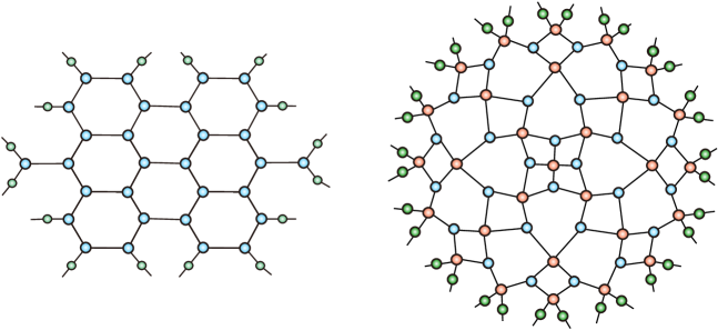
Figure 2.22: Examples of TN architectures with loops. (a) Honey-Comb Lattice (HCL) for a 16th-order tensor. (b) MERA for a 32th-order tensor.

Compared with the PEPS and PEPO formats, the main advantage of the MERA formats is that the order and size of each core tensor in the internal tensor network structure is often much smaller, which dramatically reduces the number of free parameters and provides more efficient distributed storage of huge-scale data tensors. Moreover, TNs with cycles, especially the MERA tensor network allow us to model more complex functions and interactions between variables.

2.6 Concatenated (Distributed) Representation of TT Networks

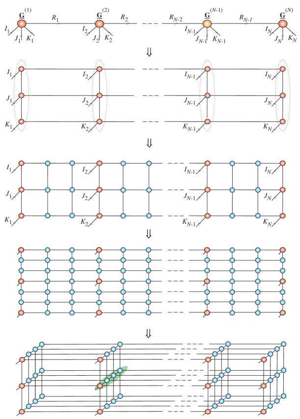
Figure 2.23: Graphical representation of a large-scale data tensor via its TT model (top panel), the PEPS model of the TT (third panel), and its transformation to a distributed 2D (second from bottom panel) and 3D (bottom panel) tensor train networks.

Complexity of algorithms for computation (contraction) on tensor networks typically scales polynomially with the rank, $R_{n}$, or size, $I_{n}$, of the core tensors, so that the computations quickly become intractable with the increase in $R_{n}$. A step towards reducing storage and computational requirements would be therefore to reduce the size (volume) of core tensors by increasing their number through distributed tensor networks (DTNs), as illustrated in Figure 2.22. The underpinning idea is that each core tensor in an original TN is replaced by another TN (see Figure 2.23 for TT networks), resulting in a distributed TN in which only some core tensors are associated with physical (natural) modes of the original data tensor [100]. A DTN consists of two kinds of relatively small-size cores (nodes), internal nodes which have no free edges and external nodes which have free edges representing natural (physical) indices of a data tensor.

The obvious advantage of DTNs is that the size of each core tensor in the internal tensor network structure is usually much smaller than the size of the initial core tensor; this allows for a better management of distributed storage, and often in the reduction of the total number of network parameters through distributed computing. However, compared to initial tree structures, the contraction of the resulting distributed tensor network becomes much more difficult because of the loops in the architecture.

2.7 Links between TNs and Machine Learning Models

Table 2.2 summarizes the conceptual connections of tensor networks with graphical and neural network models in machine learning and statistics [146, 53, 52, 110, 154, 226, 44, 45, 77]. More research is needed to establish deeper and more precise relationships.

Table 2.2: Links between tensor networks (TNs) and graphical models used in Machine Learning (ML) and Statistics. The corresponding categories are not exactly the same, but have general analogies.

Tensor Networks Neural Networks and Graphical Models in ML/Statistics TT/MPS Hidden Markov Models (HMM) HT/TTNS Deep Learning Neural Networks, Gaussian Mixture Model (GMM) PEPS Markov Random Field (MRF), Conditional Random Field (CRF) MERA Wavelets, Deep Belief Networks (DBN) ALS, DMRG/MALS Algorithms Forward-Backward Algorithms, Block Nonlinear Gauss-Seidel Methods

2.8 Changing the Structure of Tensor Networks

An advantage of the graphical (graph) representation of tensor networks is that the graphs allow us to perform complex mathematical operations on core tensors in an intuitive and easy to understand way, without the need to resort to complicated mathematical expressions. Another important advantage is the ability to modify (optimize) the topology of a TN, while keeping the original physical modes intact. The so optimized topologies yield simplified or more convenient graphical representations of a higher-order data tensor and facilitate practical applications [230, 100, 94]. In particular:

• A change in topology to a HT/TT tree structure provides reduced computational complexity, through sequential contractions of core tensors and enhanced stability of the corresponding algorithms;

• Topology of TNs with cycles can be modified so as to completely eliminate the cycles or to reduce their number;

• Even for vastly diverse original data tensors, topology modifications may produce identical or similar TN structures which make it easier to compare and jointly analyze block of interconnected data tensors. This provides opportunity to perform joint group (linked) analysis of tensors by decomposing them to TNs.

It is important to note that, due to the iterative way in which tensor contractions are performed, the computational requirements associated with tensor contractions are usually much smaller for tree-structured networks than for tensor networks containing many cycles. Therefore, for stable computations, it is advantageous to transform a tensor network with cycles into a tree structure.

Tensor Network transformations. In order to modify tensor network structures, we may perform sequential core contractions, followed by the unfolding of these contracted tensors into matrices, matrix factorizations (typically truncated SVD) and finally reshaping of such matrices back into new core tensors, as illustrated in Figures 2.24.

(a)

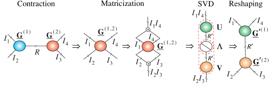
(b)

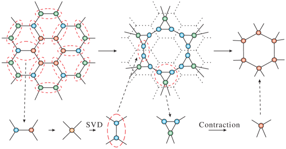
Figure 2.24: Illustration of basic transformations on a tensor network. (a) Contraction, matricization, matrix factorization (SVD) and reshaping of matrices back into tensors. (b) Transformation of a Honey-Comb lattice into a Tensor Chain (TC) via tensor contractions and the SVD.

The example in Figure 2.24(a) shows that, in the first step a contraction of two core tensors, $\underline{{\bf G}}^{(1)}\in\mathbb{R}^{I_{1}\times I_{2}\times R}$ and $\underline{{\bf G}}^{(2)}\in\mathbb{R}^{R\times I_{3}\times I_{4}}$, is performed to give the tensor

$$\underline{{\bf G}}^{(1,2)}=\underline{{\bf G}}^{(1)}\times^{1}\;\underline{{\bf G}}^{(2)}\in\mathbb{R}^{I_{1}\times I_{2}\times I_{3}\times I_{4}},$$ (2.23)

with entries $g_{i_{1},i_{2},i_{3},i_{4}}^{(1,2)}=\sum_{r=1}^{R}g_{i_{1},i_{2},r}^{(1)}\;g_{r,i_{3},i_{4}}^{(2)}$. In the next step, the tensor $\underline{{\bf G}}^{(1,2)}$ is transformed into a matrix via matricization, followed by a low-rank matrix factorization using the SVD, to give

$${\bf G}^{(1,2)}_{\overline{i_{1}i_{4}},\,\overline{i_{2}i_{3}}}\cong{\bf U}{\bf S}{\bf V}^{\text{T}}\in\mathbb{R}^{I_{1}I_{4}\times I_{2}I_{3}}.$$ (2.24)

In the final step, the factor matrices, ${\bf U}{\bf S}^{1/2}\in\mathbb{R}^{I_{1}I_{4}\times R^{\prime}}$ and ${\bf V}{\bf S}^{1/2}\in\mathbb{R}^{R^{\prime}\times I_{2}I_{3}}$, are reshaped into new core tensors, $\underline{{\bf G}}^{{}^{\prime}(1)}\in\mathbb{R}^{I_{1}\times R^{\prime}\times I_{4}}$ and $\underline{{\bf G}}^{{}^{\prime}(2)}\in\mathbb{R}^{R^{\prime}\times I_{2}\times I_{3}}$.

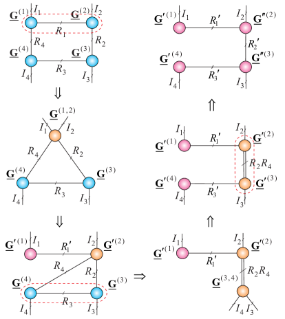
Figure 2.25: Transformation of the closed-loop Tensor Chain (TC) into the open-loop Tensor Train (TT). This is achieved by suitable contractions, reshaping and decompositions of core tensors.

The above tensor transformation procedure is quite general, and is applied in Figure 2.24(b) to transform a Honey-Comb lattice into a tensor chain (TC), while Figure 2.25 illustrates the conversion of a tensor chain (TC) into TT/MPS with OBC.

To convert a TC into TT/MPS, in the first step, we perform a contraction of two tensors, $\underline{{\bf G}}^{(1)}\in\mathbb{R}^{I_{1}\times R_{4}\times R_{1}}$ and $\underline{{\bf G}}^{(2)}\in\mathbb{R}^{R_{1}\times R_{2}\times I_{2}}$, as

$$\underline{{\bf G}}^{(1,2)}=\underline{{\bf G}}^{(1)}\times^{1}\;\underline{{\bf G}}^{(2)}\in\mathbb{R}^{I_{1}\times R_{4}\times R_{2}\times I_{2}},$$

for which the entries $g_{i_{1},r_{4},r_{2},i_{2}}^{(1,2)}=\sum_{r_{1}=1}^{R_{1}}g_{i_{1},r_{4},r_{1}}^{(1)}\;g_{r_{1},r_{2},i_{2}}^{(2)}$. In the next step, the tensor $\underline{{\bf G}}^{(1,2)}$ is transformed into a matrix, followed by a truncated SVD

$${\bf G}^{(1,2)}_{(1)}\cong{\bf U}{\bf S}{\bf V}^{\text{T}}\in\mathbb{R}^{I_{1}\times R_{4}R_{2}I_{2}}.$$

Finally, the matrices, ${\bf U}\in\mathbb{R}^{I_{1}\times R^{\prime}_{1}}$ and ${\bf V}{\bf S}\in\mathbb{R}^{R^{\prime}_{1}\times R_{4}R_{2}I_{2}}$, are reshaped back into the core tensors, $\underline{{\bf G}}^{{}^{\prime}(1)}={\bf U}\in\mathbb{R}^{1\times I_{1}\times R^{\prime}_{1}}$ and $\underline{{\bf G}}^{{}^{\prime}(2)}\in\mathbb{R}^{R^{\prime}_{1}\times R_{4}\times R_{2}\times I_{2}}$. The procedure is repeated all over again for different pairs of cores, as illustrated in Figure 2.25.

2.9 Generalized Tensor Network Formats

The fundamental TNs considered so far assume that the links between the cores are expressed by tensor contractions. In general, links between the core tensors (or tensor sub-networks) can also be expressed via other mathematical linear/multilinear or nonlinear operators, such as the outer (tensor) product, Kronecker product, Hadamard product and convolution operator. For example, the use of the outer product leads to Block Term Decomposition (BTD) [57, 61, 58, 193] and use the Kronecker products yields to the Kronecker Tensor Decomposition (KTD) [178, 174, 175]. Block term decompositions (BTD) are closely related to constrained Tucker formats (with a sparse block Tucker core) and the Hierarchical Outer Product Tensor Approximation (HOPTA), which be employed for very high-order data tensors [39].

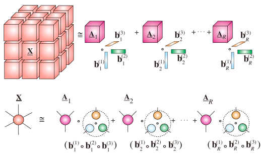
Figure 2.26: Block term decomposition (BTD) of a 6th-order block tensor, to yield $\underline{{\bf X}}=\sum_{r=1}^{R}\underline{{\bf A}}_{r}\circ\left({\bf b}_{r}^{(1)}\circ{\bf b}_{r}^{(2)}\circ{\bf b}_{r}^{(3)}\right)$ (top panel), for more detail see [57, 193]. BTD in the tensor network notation (bottom panel). Therefore, the 6th-order tensor $\underline{{\bf X}}$ is approximately represented as a sum of $R$ terms, each of which is an outer product of a 3rd-order tensor, $\underline{{\bf A}}_{r}$, and another a 3rd-order, rank-1 tensor, ${\bf b}_{r}^{(1)}\circ{\bf b}_{r}^{(2)}\circ{\bf b}_{r}^{(3)}$ (in dashed circle), which itself is an outer product of three vectors.

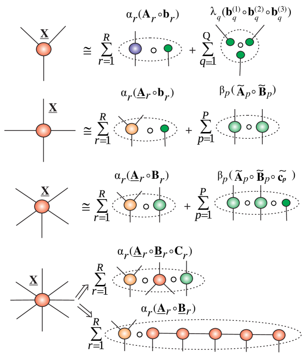
Figure 2.27: Conceptual model of the HOPTA generalized tensor network, illustrated for data tensors of different orders. For simplicity, we use the standard outer (tensor) products, but conceptually nonlinear outer products (see Eq. (2.25) and other tensor product operators (Kronecker, Hadamard) can also be employed. Each component (core tensor), $\underline{{\bf A}}_{r}$, $\underline{{\bf B}}_{r}$ and/or $\underline{{\bf C}}_{r}$, can be further hierarchically decomposed using suitable outer products, so that the HOPTA models can be applied to very high-order tensors.

Figure 2.26 illustrates such a BTD model for a 6th-order tensor, where the links between the components are expressed via outer products, while Figure 2.27 shows a more flexible Hierarchical Outer Product Tensor Approximation (HOPTA) model suitable for very high-order tensors.

Observe that the fundamental operator in the HOPTA generalized tensor networks is outer (tensor) product, which for two tensors $\underline{{\bf A}}\in\mathbb{R}^{I_{1}\times\cdots\times I_{N}}$ and $\underline{{\bf B}}\in\mathbb{R}^{J_{1}\times\cdots\times J_{M}}$, of arbitrary orders $N$ and $M$, is defined as an $(N+M)$th-order tensor $\underline{{\bf C}}=\underline{{\bf A}}\circ\underline{{\bf B}}\in\mathbb{R}^{I_{1}\times\cdots\times I_{N}\times J_{1}\times\cdots\times J_{M}}$, with entries $c_{\;i_{1},\ldots,i_{N},\,j_{1},\ldots,j_{M}}=a_{i_{1},\ldots,i_{N}}\;b_{j_{1},\ldots,j_{M}}$. This standard outer product of two tensors can be generalized to a nonlinear outer product as follows

$$\left(\underline{{\bf A}}\circ_{f}\underline{{\bf B}}\right)_{i_{1},\ldots,i_{N},j_{1},\ldots,J_{M}}=f\left(a_{i_{1},\ldots,i_{N}},b_{j_{1},\ldots,j_{M}}\right),$$ (2.25)

where $f(\cdot,\cdot)$ is a suitably designed nonlinear function with associative and commutative properties. In a similar way, we can define other nonlinear tensor products, for example, Hadamard, Kronecker or Khatri–Rao products and employ them in generalized nonlinear tensor networks. The advantage of the HOPTA model over other TN models is its flexibility and the ability to model more complex data structures by approximating very high-order tensors through a relatively small number of low-order cores.

The BTD, and KTD models can be expressed mathematically, for example, in simple nested (hierarchical) forms, given by

$$\textnormal{BTD}:\underline{{\bf X}} \cong \sum_{r=1}^{R}(\underline{{\bf A}}_{r}\circ\underline{{\bf B}}_{r}),$$ (2.26)

$$\textnormal{KTD}:\underline{\tilde{\bf X}} \cong \sum_{r=1}^{R}(\underline{{\bf A}}_{r}\otimes\underline{{\bf B}}_{r}),$$ (2.27)

where, e.g., for BTD, each factor tensor can be represented recursively as $\underline{{\bf A}}_{r}\cong\sum_{r_{1}=1}^{R_{1}}(\underline{{\bf A}}^{(1)}_{r_{1}}\circ\underline{{\bf B}}^{(1)}_{r_{1}})$ or $\underline{{\bf B}}_{r}\cong\sum_{r_{2}=1}^{R_{2}}\underline{{\bf A}}^{(2)}_{r_{2}}\circ\underline{{\bf B}}^{(2)}_{r_{2}}$.

Note that the $2N$th-order subtensors, $\underline{{\bf A}}_{r}\circ\underline{{\bf B}}_{r}$ and $\underline{{\bf A}}_{r}\otimes\underline{{\bf B}}_{r}$, have the same elements, just arranged differently. For example, if $\underline{{\bf X}}=\underline{{\bf A}}\circ\underline{{\bf B}}$ and $\underline{{\bf X}}^{\prime}=\underline{{\bf A}}\otimes\underline{{\bf B}}$, where $\underline{{\bf A}}\in\mathbb{R}^{J_{1}\times J_{2}\times\cdots\times J_{N}}$ and $\underline{{\bf B}}\in\mathbb{R}^{K_{1}\times K_{2}\times\cdots\times K_{N}}$, then
$x_{j_{1},j_{2},\ldots,j_{N},k_{1},k_{2},\ldots,k_{N}}=x^{\prime}_{k_{1}+K_{1}(j_{1}-1),\ldots,k_{N}+K_{N}(j_{N}-1)}$.

The definition of the tensor Kronecker product in the KTD model assumes that both core tensors, $\underline{{\bf A}}_{r}$ and $\underline{{\bf B}}_{r}$, have the same order. This is not a limitation, given that vectors and matrices can also be treated as tensors, e.g, a matrix of dimension $I\times J$ as is also a 3rd-order tensor of dimension $I\times J\times 1$. In fact, from the BTD/KTD models, many existing and new TDs/TNs can be derived by changing the structure and orders of factor tensors, $\underline{{\bf A}}_{r}$ and $\underline{{\bf B}}_{r}$. For example:

• If $\underline{{\bf A}}_{r}$ are rank-1 tensors of size $I_{1}\times I_{2}\times\cdots\times I_{N}$, and $\underline{{\bf B}}_{r}$ are scalars,   $\forall r$, then (2.27) represents the rank-$R$ CP decomposition;

• If $\underline{{\bf A}}_{r}$ are rank-$L_{r}$ tensors of size $I_{1}\times I_{2}\times\cdots\times I_{R}\times 1\times\cdots\times 1$, in the Kruskal (CP) format, and $\underline{{\bf B}}_{r}$ are rank-1 tensors of size $1\times\cdots\times 1\times I_{R+1}\times\cdots\times I_{N}$,   $\forall r$, then (2.27) expresses the rank-($L_{r}\circ 1$) BTD;

• If $\underline{{\bf A}}_{r}$ and $\underline{{\bf B}}_{r}$ are expressed by KTDs, we arrive at the Nested Kronecker Tensor Decomposition (NKTD), a special case of which is the Tensor Train (TT) decomposition. Therefore, the BTD model in (2.27) can also be used for recursive TT-decompositions.

The generalized tensor network approach caters for a large variety of tensor decomposition models, which may find applications in scientific computing, signal processing or deep learning (see, eg., [58, 37, 39, 177, 45]).

In this monograph, we will mostly focus on the more established Tucker and TT decompositions (and some of their extensions), due to their conceptual simplicity, availability of stable and efficient algorithms for their computation and the possibility to naturally extend these models to more complex tensor networks. In other words, the Tucker and TT models are considered here as simplest prototypes, which can then serve as building blocks for more sophisticated tensor networks.

Chapter 3 Constrained Tensor Decompositions: From Two-way to Multiway Component Analysis

The component analysis (CA) framework usually refers to the application of constrained matrix factorization techniques to observed mixed signals in order to extract components with specific properties and/or estimate the mixing matrix [40, 43, 47, 55, 103]. In the machine learning practice, to aid the well-posedness and uniqueness of the problem, component analysis methods exploit prior knowledge about the statistics and diversities of latent variables (hidden sources) within the data. Here, by the diversities, we refer to different characteristics, features or morphology of latent variables which allow us to extract the desired components or features, for example, sparse or statistically independent components.

3.1 Constrained Low-Rank Matrix Factorizations

Two-way Component Analysis (2-way CA), in its simplest form, can be formulated as a constrained matrix factorization of typically low-rank, in the form

$${\bf X}={\bf A}\mbox{\boldmath$\Lambda$}{\bf B}^{\text{T}}+{\bf E}=\sum_{r=1}^{R}\lambda_{r}\;{\bf a}_{r}\circ{\bf b}_{r}+{\bf E}=\sum_{r=1}^{R}\lambda_{r}\,{\bf a}_{r}\,{\bf b}^{\text{T}}_{r}+{\bf E},$$ (3.1)

where $\mbox{\boldmath$\Lambda$}=\mbox{diag}(\lambda_{1},\ldots,\lambda_{R})$ is an optional diagonal scaling matrix. The potential constraints imposed on the factor matrices, ${\bf A}$ and/or ${\bf B}$, include orthogonality, sparsity, statistical independence, nonnegativity or smoothness. In the bilinear 2-way CA in (3.1), ${\bf X}\in\mathbb{R}^{I\times J}$ is a known matrix of observed data, ${\bf E}\in\mathbb{R}^{I\times J}$ represents residuals or noise, ${\bf A}=[{\bf a}_{1},{\bf a}_{2},\ldots,{\bf a}_{R}]\in\mathbb{R}^{I\times R}$ is the unknown mixing matrix with $R$ basis vectors ${\bf a}_{r}\in\mathbb{R}^{I}$, and depending on application, ${\bf B}=[{\bf b}_{1},{\bf b}_{2},$ $\ldots,{\bf b}_{R}]$ $\in\mathbb{R}^{J\times R}$, is the matrix of unknown components, factors, latent variables, or hidden sources, represented by vectors ${\bf b}_{r}\in\mathbb{R}^{J}$ (see Figure 3.2).

It should be noted that 2-way CA has an inherent symmetry. Indeed, Eq. (3.1) could also be written as ${\bf X}^{\text{T}}\approx{\bf B}{\bf A}^{\text{T}}$, thus interchanging the roles of sources and mixing process.

Algorithmic approaches to 2-way (matrix) component analysis are well established, and include Principal Component Analysis (PCA), Robust PCA (RPCA), Independent Component Analysis (ICA), Nonnegative Matrix Factorization (NMF), Sparse Component Analysis (SCA) and Smooth Component Analysis (SmCA) [6, 43, 24, 47, 109, 228]. These techniques have become standard tools in blind source separation (BSS), feature extraction, and classification paradigms. The columns of the matrix ${\bf B}$, which represent different latent components, are then determined by specific chosen constraints and should be, for example, (i) as statistically mutually independent as possible for ICA; (ii) as sparse as possible for SCA; (iii) as smooth as possible for SmCA; (iv) take only nonnegative values for NMF.

Singular value decomposition (SVD) of the data matrix ${\bf X}\in\mathbb{R}^{I\times J}$ is a special, very important, case of the factorization in Eq. (3.1), and is given by

$${\bf X}={\bf U}{\bf S}{\bf V}^{\text{T}}=\sum_{r=1}^{R}\sigma_{r}\;{\bf u}_{r}\circ{\bf v}_{r}=\sum_{r=1}^{R}\sigma_{r}\;{\bf u}_{r}{\bf v}_{r}^{\text{T}},$$ (3.2)

where ${\bf U}\in\mathbb{R}^{I\times R}$ and ${\bf V}\in\mathbb{R}^{J\times R}$ are column-wise orthogonal matrices and ${\bf S}\in\mathbb{R}^{R\times R}$ is a diagonal matrix containing only nonnegative singular values $\sigma_{r}$ in a monotonically non-increasing order.

According to the well known Eckart–Young theorem, the truncated SVD provides the optimal, in the least-squares (LS) sense, low-rank matrix approximation. The SVD, therefore, forms the backbone of low-rank matrix approximations (and consequently low-rank tensor approximations).

Another virtue of component analysis comes from the ability to perform simultaneous matrix factorizations

$${\bf X}_{k}\approx{\bf A}_{k}{\bf B}_{k}^{\text{T}},\qquad(k=1,2,\ldots,K),$$ (3.3)

on several data matrices, ${\bf X}_{k}$, which represent linked datasets, subject to various constraints imposed on linked (interrelated) component (factor) matrices. In the case of orthogonality or statistical independence constraints, the problem in (3.3) can be related to models of group PCA/ICA through suitable pre-processing, dimensionality reduction and post-processing procedures [75, 88, 38, 191, 239]. The terms “group component analysis” and “joint multi-block data analysis” are used interchangeably to refer to methods which aim to identify links (correlations, similarities) between hidden components in data. In other words, the objective of group component analysis is to analyze the correlation, variability, and consistency of the latent components across multi-block datasets. The field of 2-way CA is maturing and has generated efficient algorithms for 2-way component analysis, especially for sparse/functional PCA/SVD, ICA, NMF and SCA [6, 40, 47, 236, 103].

The rapidly emerging field of tensor decompositions is the next important step which naturally generalizes 2-way CA/BSS models and algorithms. Tensors, by virtue of multilinear algebra, offer enhanced flexibility in CA, in the sense that not all components need to be statistically independent, and can be instead smooth, sparse, and/or non-negative (e.g., spectral components). Furthermore, additional constraints can be used to reflect physical properties and/or diversities of spatial distributions, spectral and temporal patterns. We proceed to show how constrained matrix factorizations or 2-way CA models can be extended to multilinear models using tensor decompositions, such as the Canonical Polyadic (CP) and the Tucker decompositions, as illustrated in Figures 3.1, 3.2 and 3.3.

3.2 The CP Format

The CP decomposition (also called the CANDECOMP, PARAFAC, or Canonical Polyadic decomposition) decomposes an $N$th-order tensor, $\underline{{\bf X}}\in\mathbb{R}^{I_{1}\times I_{2}\times\cdots\times I_{N}}$, into a linear combination of terms, ${\bf b}^{(1)}_{r}\circ{\bf b}^{(2)}_{r}\circ\cdots\circ{\bf b}^{(N)}_{r}$, which are rank-1 tensors, and is given by [96, 95, 29]

$$\underline{{\bf X}} \cong\sum_{r=1}^{R}\lambda_{r}\;{\bf b}^{(1)}_{r}\circ{\bf b}^{(2)}_{r}\circ\cdots\circ{\bf b}^{(N)}_{r}$$ (3.4)

$$=\underline{\mbox{\boldmath$\Lambda$}}\times_{1}{\bf B}^{(1)}\times_{2}{\bf B}^{(2)}\cdots\times_{N}{\bf B}^{(N)}$$

$$=\llbracket\underline{\mbox{\boldmath$\Lambda$}};\mathbf{B}^{(1)},\mathbf{B}^{(2)},\ldots,\mathbf{B}^{(N)}\rrbracket,$$

where $\lambda_{r}$ are non-zero entries of the diagonal core tensor $\underline{\mbox{\boldmath$\Lambda$}}\in\mathbb{R}^{R\times R\times\cdots\times R}$ and ${\bf B}^{(n)}=[{\bf b}_{1}^{(n)},{\bf b}_{2}^{(n)},\ldots,{\bf b}_{R}^{(n)}]\in\mathbb{R}^{I_{n}\times R}$ are factor matrices (see Figure 3.1 and Figure 3.2).

Via the Khatri–Rao products (see Table 2.1), the CP decomposition can be equivalently expressed in a matrix/vector form as

$${\bf X}_{(n)} \cong {\bf B}^{(n)}\mbox{\boldmath$\Lambda$}({\bf B}^{(N)}\odot\cdots\odot{\bf B}^{(n+1)}\odot{\bf B}^{(n-1)}\odot\cdots\odot{\bf B}^{(1)})^{\text{T}}$$

$$= {\bf B}^{(n)}\mbox{\boldmath$\Lambda$}({\bf B}^{(1)}\odot_{L}\cdots\odot_{L}{\bf B}^{(n-1)}\odot_{L}{\bf B}^{(n+1)}\odot_{L}\cdots\odot_{L}{\bf B}^{(N)})^{\text{T}}$$

and

$$\text{vec}(\underline{{\bf X}}) \cong [{\bf B}^{(N)}\odot{\bf B}^{(N-1)}\odot\cdots\odot{\bf B}^{(1)}]\;\mbox{\boldmath$\lambda$}$$

$$\cong [{\bf B}^{(1)}\odot_{L}{\bf B}^{(2)}\odot_{L}\cdots\odot_{L}{\bf B}^{(N)}]\;\mbox{\boldmath$\lambda$},$$

where $\mbox{\boldmath$\lambda$}=[\lambda_{1},\lambda_{2},\ldots,\lambda_{R}]^{\text{T}}$ and $\mbox{\boldmath$\Lambda$}=\mathop{\rm diag}\nolimits(\lambda_{1},\ldots,\lambda_{R})$ is a diagonal matrix.

(a) Standard block diagram for CP decomposition of a 3rd-order tensor

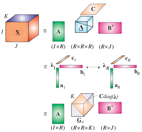
(b) CP decomposition for a 4th-order tensor in the tensor network notation

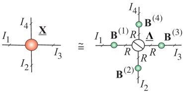
Figure 3.1: Representations of the CP decomposition. The objective of the CP decomposition is to estimate the factor matrices ${\bf B}^{(n)}\in\mathbb{R}^{I_{n}\times R}$ and scaling coefficients $\{\lambda_{1},\lambda_{1},\ldots,\lambda_{R}\}$. (a) The CP decomposition of a 3rd-order tensor in the form, $\underline{{\bf X}}\cong\underline{\mbox{\boldmath$\Lambda$}}\times_{1}{\bf A}\times_{2}{\bf B}\times_{3}{\bf C}=\sum_{r=1}^{R}\lambda_{r}\;{\bf a}_{r}\circ{\bf b}_{r}\circ{\bf c}_{r}=\underline{{\bf G}}_{c}\times_{1}{\bf A}\times_{2}{\bf B}$, with $\underline{{\bf G}}_{c}=\underline{\mbox{\boldmath$\Lambda$}}\times_{3}{\bf C}$. (b) The CP decomposition for a 4th-order tensor in the form $\underline{{\bf X}}\cong\underline{\mbox{\boldmath$\Lambda$}}\times_{1}{\bf B}^{(1)}\times_{2}{\bf B}^{(2)}\times_{3}{\bf B}^{(3)}\times_{4}{\bf B}^{(4)}=\sum_{r=1}^{R}\lambda_{r}\;{\bf b}^{(1)}_{r}\circ{\bf b}^{(2)}_{r}\circ{\bf b}^{(3)}_{r}\circ{\bf b}^{(4)}_{r}$.

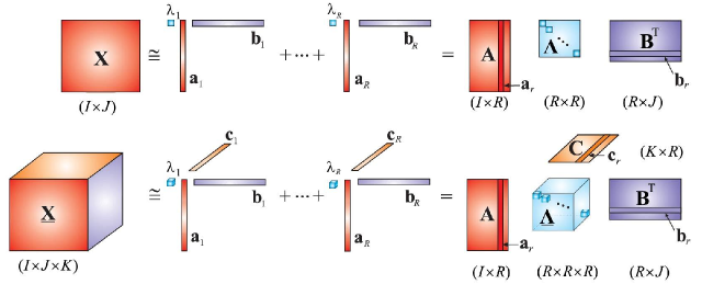
Figure 3.2: Analogy between a low-rank matrix factorization, ${\bf X}\cong{\bf A}\mbox{\boldmath$\Lambda$}{\bf B}^{\text{T}}=\sum_{r=1}^{R}\lambda_{r}\;{\bf a}_{r}\circ{\bf b}_{r}$ (top), and a simple low-rank tensor factorization (CP decomposition), $\underline{{\bf X}}\cong\underline{\mbox{\boldmath$\Lambda$}}\times_{1}{\bf A}\times_{2}{\bf B}\times_{3}{\bf C}=\sum_{r=1}^{R}\lambda_{r}\;{\bf a}_{r}\circ{\bf b}_{r}\circ{\bf c}_{r}$ (bottom).

The rank of a tensor $\underline{{\bf X}}$ is defined as the smallest $R$ for which the CP decomposition in (3.4) holds exactly.

Algorithms to compute CP decomposition. In real world applications, the signals of interest are corrupted by noise, so that the CP decomposition is rarely exact and has to be estimated by minimizing a suitable cost function. Such cost functions are typically of the Least-Squares (LS) type, in the form of the Frobenius norm

$$J_{2}(\mathbf{B}^{(1)},\mathbf{B}^{(2)},\ldots,\mathbf{B}^{(N)})=\|\underline{{\bf X}}-\llbracket\underline{\mbox{\boldmath$\Lambda$}};\mathbf{B}^{(1)},\mathbf{B}^{(2)},\ldots,\mathbf{B}^{(N)}\rrbracket\|^{2}_{F},$$ (3.7)

or Least Absolute Error (LAE) criteria [217]

$$J_{1}(\mathbf{B}^{(1)},\mathbf{B}^{(2)},\ldots,\mathbf{B}^{(N)})=\|\underline{{\bf X}}-\llbracket\underline{\mbox{\boldmath$\Lambda$}};\mathbf{B}^{(1)},\mathbf{B}^{(2)},\ldots,\mathbf{B}^{(N)}\rrbracket\|_{1}.$$ (3.8)

The Alternating Least Squares (ALS) based algorithms minimize the cost function iteratively by individually optimizing each component (factor matrix, ${\bf B}^{(n)}$)), while keeping the other component matrices fixed [95, 119].

To illustrate the ALS principle, assume that the diagonal matrix $\Lambda$ has been absorbed into one of the component matrices; then, by taking advantage of the Khatri–Rao structure in Eq. (3.2), the component matrices, ${\bf B}^{(n)}$, can be updated sequentially as

$${\bf B}^{(n)}\leftarrow{\bf X}_{(n)}\left(\bigodot_{k\neq n}{\bf B}^{(k)}\right)\left(\bigoasterisk_{k\neq n}({\bf B}^{(k)\;\text{T}}{\bf B}^{(k)})\right)^{\dagger}.$$ (3.9)

The main challenge (or bottleneck) in implementing ALS and Gradient Decent (GD) techniques for CP decomposition lies therefore in multiplying a matricized tensor and Khatri–Rao product (of factor matrices) [171, 35] and in the computation of the pseudo-inverse of $(R\times R)$ matrices (for the basic ALS see Algorithm 1).

0:  Data tensor $\underline{{\bf X}}\in\mathbb{R}^{I\times J\times K}$ and rank $R$ 0:  Factor matrices ${\bf A}\in\mathbb{R}^{I\times R}$, ${\bf B}\in\mathbb{R}^{J\times R}$, ${\bf C}\in\mathbb{R}^{K\times R}$, and scaling vector $\mbox{\boldmath$\lambda$}\in\mathbb{R}^{R}$ 1:  Initialize ${\bf A},{\bf B},{\bf C}$ 2:  while not converged or iteration limit is not reached do 3:     ${\bf A}\leftarrow{\bf X}_{(1)}({\bf C}\odot{\bf B})({\bf C}^{\text{T}}{\bf C}\circledast{\bf B}^{\text{T}}{\bf B})^{\dagger}$ 4:     Normalize column vectors of ${\bf A}$ to unit length (by computing the norm of each column vector and dividing each element of a vector by its norm) 5:     ${\bf B}\leftarrow{\bf X}_{(2)}({\bf C}\odot{\bf A})({\bf C}^{\text{T}}{\bf C}\circledast{\bf A}^{\text{T}}{\bf A})^{\dagger}$ 6:     Normalize column vectors of ${\bf B}$ to unit length 7:     ${\bf C}\leftarrow{\bf X}_{(3)}({\bf B}\odot{\bf A})({\bf B}^{\text{T}}{\bf B}\circledast{\bf C}^{\text{T}}{\bf C})^{\dagger}$ 8:     Normalize column vectors of ${\bf C}$ to unit length, store the norms in vector $\lambda$ 9:  end while 10:  return  ${\bf A},{\bf B},{\bf C}$ and $\lambda$.

Algorithm 1 Basic ALS for the CP decomposition of a 3rd-order tensor

The ALS approach is attractive for its simplicity, and often provides satisfactory performance for well defined problems with high SNRs and well separated and non-collinear components. For ill-conditioned problems, advanced algorithms are required which typically exploit the rank-1 structure of the terms within CP decomposition to perform efficient computation and storage of the Jacobian and Hessian of the cost function [176, 193, 172]. Implementation of parallel ALS algorithm over distributed memory for very large-scale tensors was proposed in [35, 108].

Multiple random projections, tensor sketching and Giga-Tensor. Most of the existing algorithms for the computation of CP decomposition are based on the ALS or GD approaches, however, these can be too computationally expensive for huge tensors. Indeed, algorithms for tensor decompositions have generally not yet reached the level of maturity and efficiency of low-rank matrix factorization (LRMF) methods. In order to employ efficient LRMF algorithms to tensors, we need to either: (i) reshape the tensor at hand into a set of matrices using traditional matricizations, (ii) employ reduced randomized unfolding matrices, or (iii) perform suitable random multiple projections of a data tensor onto lower-dimensional subspaces. The principles of the approaches (i) and (ii) are self-evident, while the approach (iii) employs a multilinear product of an $N$th-order tensor and $(N-2)$ random vectors, which are either chosen uniformly from a unit sphere or assumed to be i.i.d. Gaussian vectors [126].

For example, for a 3rd-order tensor, $\underline{{\bf X}}\in\mathbb{R}^{I_{1}\times I_{2}\times I_{3}}$, we can use the set of random projections, ${\bf X}_{\bar{3}}=\underline{{\bf X}}\;\bar{\times}_{3}\;\mbox{\boldmath$\omega$}_{3}\in\mathbb{R}^{I_{1}\times I_{2}}$, ${\bf X}_{\bar{2}}=\underline{{\bf X}}\;\bar{\times}_{2}\;\mbox{\boldmath$\omega$}_{2}\in\mathbb{R}^{I_{1}\times I_{3}}$ and ${\bf X}_{\bar{1}}=\underline{{\bf X}}\;\bar{\times}_{1}\;\mbox{\boldmath$\omega$}_{1}\in\mathbb{R}^{I_{2}\times I_{3}}$, where the vectors $\mbox{\boldmath$\omega$}_{n}\in\mathbb{R}^{I_{n}}$, $\,n=1,2,3$, are suitably chosen random vectors. Note that random projections in such a case are non-typical – instead of using projections for dimensionality reduction, they are used to reduce a tensor of any order to matrices and consequently transform the CP decomposition problem to constrained matrix factorizations problem, which can be solved via simultaneous (joint) matrix diagonalization [56, 31]. It was shown that even a small number of random projections, such as ${\cal{O}}(\log R)$ is sufficient to preserve the spectral information in a tensor. This mitigates the problem of the dependence on the eigen-gap that plagued earlier tensor-to-matrix reductions. Although a uniform random sampling may experience problems for tensors with spiky elements, it often outperforms the standard CP-ALS decomposition algorithms.

Alternative algorithms for the CP decomposition of huge-scale tensors include tensor sketching – a random mapping technique, which exploits kernel methods and regression [168, 223], and the class of distributed algorithms such as the DFacTo [35] and the GigaTensor which is based on Hadoop / MapReduce paradigm [106].

Constraints. Under rather mild conditions, the CP decomposition is generally unique by itself [125, 188]. It does not require additional constraints on the factor matrices to achieve uniqueness, which makes it a powerful and useful tool for tensor factroization. Of course, if the components in one or more modes are known to possess some properties, e.g., they are known to be nonnegative, orthogonal, statistically independent or sparse, such prior knowledge may be incorporated into the algorithms to compute CPD and at the same time relax uniqueness conditions. More importantly, such constraints may enhance the accuracy and stability of CP decomposition algorithms and also facilitate better physical interpretability of the extracted components [187, 65, 195, 117, 234, 134].

Applications. The CP decomposition has already been established as an advanced tool for blind signal separation in vastly diverse branches of signal processing and machine learning [1, 119, 147, 3, 223, 207, 189]. It is also routinely used in exploratory data analysis, where the rank-1 terms capture essential properties of dynamically complex datasets, while in wireless communication systems, signals transmitted by different users correspond to rank-1 terms in the case of line-of-sight propagation and therefore admit analysis in the CP format. Another potential application is in harmonic retrieval and direction of arrival problems, where real or complex exponentials have rank-1 structures, for which the use of CP decomposition is quite natural [185, 186, 194].

3.3 The Tucker Tensor Format

Compared to the CP decomposition, the Tucker decomposition provides a more general factorization of an $N$th-order tensor into a relatively small size core tensor and factor matrices, and can be expressed as follows:

$$\underline{{\bf X}} \cong \sum\limits_{r_{1}=1}^{R_{1}}{{\cdots\sum\limits_{r_{N}=1}^{R_{N}}{g_{r_{1}r_{2}\cdots r_{N}}\,\left(\;{\bf b}^{(1)}_{r_{1}}\circ{\bf b}^{(2)}_{r_{2}}\circ\cdots\circ{\bf b}^{(N)}_{r_{N}}\right)}}}$$ (3.10)

$$= \underline{{\bf G}}\times_{1}{\bf B}^{(1)}\times_{2}{\bf B}^{(2)}\cdots\times_{N}{\bf B}^{(N)}$$

$$= \llbracket\underline{{\bf G}};{\bf B}^{(1)},{\bf B}^{(2)},\ldots,{\bf B}^{(N)}\rrbracket,$$

where $\underline{{\bf X}}\in\mathbb{R}^{I_{1}\times I_{2}\times\cdots\times I_{N}}$ is the given data tensor, $\underline{{\bf G}}\in\mathbb{R}^{R_{1}\times R_{2}\times\cdots\times R_{N}}$ is the core tensor, and ${\bf B}^{(n)}=[{\bf b}_{1}^{(n)},{\bf b}_{2}^{(n)},\ldots,{\bf b}_{R_{n}}^{(n)}]\in\mathbb{R}^{I_{n}\times R_{n}}$ are the mode-$n$ factor (component) matrices, $n=1,2,\ldots,N$ (see Figure 3.3). The core tensor (typically, $R_{n}<<I_{n}$) models a potentially complex pattern of mutual interaction between the vectors in different modes. The model in (3.10) is often referred to as the Tucker-$N$ model.

The CP and Tucker decompositions have long history. For recent surveys and more detailed information we refer to [119, 87, 46, 42, 189].

Using the properties of the Kronecker tensor product, the Tucker-$N$ decomposition in (3.10) can be expressed in an equivalent matrix and vector form as

$${\bf X}_{(n)} \cong{\bf B}^{(n)}{\bf G}_{(n)}({\bf B}^{(1)}\otimes_{L}\cdots\otimes_{L}{\bf B}^{(n-1)}\otimes_{L}{\bf B}^{(n+1)}\otimes_{L}\cdots\otimes_{L}{\bf B}^{(N)})^{\text{T}}$$

$$={\bf B}^{(n)}{\bf G}_{(n)}({\bf B}^{(N)}\otimes\cdots\otimes{\bf B}^{(n+1)}\otimes{\bf B}^{(n-1)}\otimes\cdots\otimes{\bf B}^{(1)})^{\text{T}},$$ (3.11)

$${\bf X}_{<n>} \cong({\bf B}^{(1)}\otimes_{L}\cdots\otimes_{L}{\bf B}^{(n)})\;{\bf G}_{<n>}({\bf B}^{(n+1)}\otimes_{L}\cdots\otimes_{L}{\bf B}^{(N)})^{\text{T}}$$

$$=({\bf B}^{(n)}\otimes\cdots\otimes{\bf B}^{(1)})\;{\bf G}_{<n>}({\bf B}^{(N)}\otimes{\bf B}^{(N-1)}\otimes\cdots\otimes{\bf B}^{(n+1)})^{\text{T}},$$

$$\text{vec}(\underline{{\bf X}}) \cong[{\bf B}^{(1)}\otimes_{L}{\bf B}^{(2)}\otimes_{L}\cdots\otimes_{L}{\bf B}^{(N)}]\;\text{vec}(\underline{{\bf G}})$$

$$=[{\bf B}^{(N)}\otimes{\bf B}^{(N-1)}\otimes\cdots\otimes{\bf B}^{(1)}]\;\text{vec}(\underline{{\bf G}}),$$ (3.13)

where the multi-indices are ordered in a reverse lexicographic order (little-endian).

Table 3.1 and Table 3.2 summarize fundamental mathematical representations of CP and Tucker decompositions for 3rd-order and $N$th-order tensors.

(a) Standard block diagrams of Tucker (top) and Tucker-CP (bottom) decompositions for a 3rd-order tensor

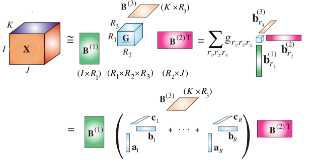
(b) The TN diagram for the Tucker and Tucker/CP decompositions of a 4th-order tensor

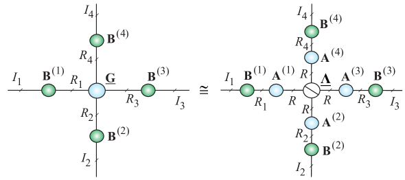
Figure 3.3: Illustration of the Tucker and Tucker-CP decompositions, where the objective is to compute the factor matrices, ${\bf B}^{(n)}$, and the core tensor, $\underline{{\bf G}}$. (a) Tucker decomposition of a 3rd-order tensor, $\underline{{\bf X}}\cong\underline{{\bf G}}\times_{1}{\bf B}^{(1)}\times_{2}{\bf B}^{(2)}\times_{3}{\bf B}^{(3)}$. In some applications, the core tensor can be further approximately factorized using the CP decomposition as $\underline{{\bf G}}\cong\sum_{r=1}^{R}{\bf a}_{r}\circ{\bf b}_{r}\circ{\bf c}_{r}$ (bottom diagram), or alternatively using TT/HT decompositions. (b) Graphical representation of the Tucker-CP decomposition for a 4th-order tensor, $\underline{{\bf X}}\cong\underline{{\bf G}}\times_{1}{\bf B}^{(1)}\times_{2}{\bf B}^{(2)}\times_{3}{\bf B}^{(3)}\times_{4}{\bf B}^{(4)}=\llbracket\underline{{\bf G}};{\bf B}^{(1)},{\bf B}^{(2)},{\bf B}^{(3)},{\bf B}^{(4)}\rrbracket\cong(\underline{\mbox{\boldmath$\Lambda$}}\times_{1}{\bf A}^{(1)}\times_{2}{\bf A}^{(2)}\times_{3}{\bf A}^{(3)}\times_{4}{\bf A}^{(4)})\times_{1}{\bf B}^{(1)}\times_{2}{\bf B}^{(2)}\times_{3}{\bf B}^{(3)}\times_{4}{\bf B}^{(4)}=\llbracket\underline{\mbox{\boldmath$\Lambda$}};\;{\bf B}^{(1)}{\bf A}^{(1)},\;{\bf B}^{(2)}{\bf A}^{(2)},\;{\bf B}^{(3)}{\bf A}^{(3)},\;{\bf B}^{(4)}{\bf A}^{(4)}\rrbracket$.

The Tucker decomposition is said to be in an independent Tucker format if all the factor matrices, ${\bf B}^{(n)}$, are full column rank, while a Tucker format is termed an orthonormal format, if in addition, all the factor matrices, ${\bf B}^{(n)}={\bf U}^{(n)}$, are orthogonal. The standard Tucker model often has orthogonal factor matrices.

Multilinear rank. The multilinear rank of an $N$th-order tensor $\underline{{\bf X}}\in\mathbb{R}^{I_{1}\times I_{2}\times\cdots\times I_{N}}$ corresponds to the $N$-tuple $(R_{1},R_{2},\ldots,R_{N})$ consisting of the dimensions of the different subspaces. If the Tucker decomposition (3.10) holds exactly it is mathematically defined as

$$\mbox{rank}_{ML}(\underline{{\bf X}})=\{\mbox{rank}({\bf X}_{(1)}),\mbox{rank}({\bf X}_{(2)}),\ldots,\mbox{rank}({\bf X}_{(N)})\},$$ (3.14)

with ${\bf X}_{(n)}\in\mathbb{R}^{I_{n}\times I_{1}\cdots I_{n-1}I_{n+1}\cdots I_{N}}$ for $n=1,2,\ldots,N$. Rank of the Tucker decompositions can be determined using information criteria [227], or through the number of dominant eigenvalues when an approximation accuracy of the decomposition or a noise level is given (see Algorithm 8).

The independent Tucker format has the following important properties if the equality in (3.10) holds exactly (see, e.g., [105] and references therein):

1. The tensor (CP) rank of any tensor, $\underline{{\bf X}}=\llbracket\underline{{\bf G}};{\bf B}^{(1)},{\bf B}^{(2)},\ldots,{\bf B}^{(N)}\rrbracket\in\mathbb{R}^{I_{1}\times I_{2}\times\cdots\times I_{N}}$, and the rank of its core tensor, $\underline{{\bf G}}\in\mathbb{R}^{R_{1}\times R_{2}\times\cdots\times R_{N}}$, are exactly the same, i.e.,

   $$\mbox{rank}_{CP}(\underline{{\bf X}})=\mbox{rank}_{CP}(\underline{{\bf G}}).$$ (3.15)

2. If a tensor, $\underline{{\bf X}}\in\mathbb{R}^{I_{1}\times I_{2}\times\cdots\times I_{N}}=\llbracket\underline{{\bf G}};{\bf B}^{(1)},{\bf B}^{(2)},\ldots,{\bf B}^{(N)}\rrbracket$, admits an independent Tucker format with multilinear rank $\{R_{1},R_{2},\ldots,R_{N}\}$, then

   $$R_{n}\leq\prod_{p\neq n}^{N}R_{p}\quad\forall n.$$ (3.16)

   Moreover, without loss of generality, under the assumption $R_{1}\leq R_{2}\leq\cdots\leq R_{N}$, we have

   $$R_{1}\leq\mbox{rank}_{CP}(\underline{{\bf X}})\leq R_{2}R_{3}\cdots R_{N}.$$ (3.17)

3. If a data tensor is symmetric and admits an independent Tucker format, $\underline{{\bf X}}=\llbracket\underline{{\bf G}};{\bf B},{\bf B},\ldots,{\bf B}\rrbracket\in\mathbb{R}^{I\times I\times\cdots\times I}$, then its core tensor, $\underline{{\bf G}}\in\mathbb{R}^{R\times R\times\cdots\times R}$, is also symmetric, with $\mbox{rank}_{CP}(\underline{{\bf X}})=\mbox{rank}_{CP}(\underline{{\bf G}}$).

4. For the orthonormal Tucker format, that is, $\underline{{\bf X}}=\llbracket\underline{{\bf G}};{\bf U}^{(1)},{\bf U}^{(2)},\ldots,{\bf U}^{(N)}\rrbracket\in\mathbb{R}^{I_{1}\times I_{2}\times\cdots\times I_{N}}$, with ${\bf U}^{(n)\text{T}}\,{\bf U}^{(n)}={\bf I},\,\forall n$, the Frobenius norms and the Schatten $p$-norms of the data tensor, $\underline{{\bf X}}$ , and its core tensor, $\underline{{\bf G}}$, are equal, i.e.,

   $$\|\underline{{\bf X}}\|_{F} = \|\underline{{\bf G}}\|_{F},$$

   $$\|\underline{{\bf X}}\|_{{\cal{S}}_{p}} = \|\underline{{\bf G}}\|_{{\cal{S}}_{p}},\quad 1\leq p<\infty.$$

   Thus, the computation of the Frobenius norms can be performed with an ${\cal{O}}(R^{N})$ complexity $(R=\max\{R_{1},\ldots,R_{N}\})$, instead of the usual order ${\cal{O}}(I^{N})$ complexity (typically $R\ll I$).

Table 3.1: Different forms of CP and Tucker representations of a 3rd-order tensor $\underline{{\bf X}}\in\mathbb{R}^{I\times J\times K}$, where $\;\mbox{\boldmath$\lambda$}=[\lambda_{1},\lambda_{2},\ldots,\lambda_{R}]^{\text{T}}$, and $\;\mbox{\boldmath$\Lambda$}=\mbox{diag}\{\lambda_{1},\lambda_{2},\ldots,\lambda_{R}\}$.

      CP Decomposition Tucker Decomposition Scalar representation $x_{ijk}=\sum\limits_{r=1}^{R}{\lambda_{r}\,a_{i\,r}\,b_{j\,r}\,c_{k\,r}}$      $\quad x_{ijk}=\sum\limits_{r_{1}=1}^{R_{1}}\sum\limits_{r_{2}=1}^{R_{2}}\sum\limits_{r_{3}=1}^{R_{3}}{g_{r_{1}\,r_{2}\,r_{3}}\;a_{i\,r_{1}}\,b_{j\,r_{2}}\,c_{k\,r_{3}}}$ Tensor representation, outer products $\;\;\underline{{\bf X}}=\sum\limits_{r=1}^{R}{\lambda_{r}\;{\bf a}_{r}\circ{\bf b}_{r}\circ{\bf c}_{r}}$      $\;\;\quad\underline{{\bf X}}=\sum\limits_{r_{1}=1}^{R_{1}}\sum\limits_{r_{2}=1}^{R_{2}}\sum\limits_{r_{3}=1}^{R_{3}}{g_{r_{1}\,r_{2}\,r_{3}}\;{\bf a}_{r_{1}}\circ{\bf b}_{r_{2}}\circ{\bf c}_{r_{3}}}$ Tensor representation, multilinear products $\;\;\underline{{\bf X}}=\underline{\mbox{\boldmath$\Lambda$}}\times_{1}{\bf A}\times_{2}{\bf B}\times_{3}{\bf C}$ $\underline{{\bf X}}=\underline{{\bf G}}\times_{1}{\bf A}\times_{2}{\bf B}\times_{3}{\bf C}$ $\;\;\quad=\llbracket\underline{\mbox{\boldmath$\Lambda$}};\;{\bf A},\;{\bf B},\;{\bf C}\rrbracket$ $\quad=\llbracket\underline{{\bf G}};\;{\bf A},\;{\bf B},\;{\bf C}\rrbracket$ Matrix representations $\;\;{\bf X}_{(1)}={\bf A}\;\mbox{\boldmath$\Lambda$}\;({\bf B}\odot_{L}{\bf C})^{\text{T}}$ ${\bf X}_{(1)}={\bf A}\;{\bf G}_{(1)}\;({\bf B}\otimes_{L}{\bf C})^{\text{T}}$ $\;\;{\bf X}_{(2)}={\bf B}\;\mbox{\boldmath$\Lambda$}\;({\bf A}\odot_{L}{\bf C})^{\text{T}}$ ${\bf X}_{(2)}={\bf B}\;{\bf G}_{(2)}\;({\bf A}\otimes_{L}{\bf C})^{\text{T}}$ $\;\;{\bf X}_{(3)}={\bf C}\;\mbox{\boldmath$\Lambda$}\;({\bf A}\odot_{L}{\bf B})^{\text{T}}$ ${\bf X}_{(3)}={\bf C}\;{\bf G}_{(3)}\;({\bf A}\otimes_{L}{\bf B})^{\text{T}}$ Vector representation $\;\;\text{vec}(\underline{{\bf X}})=({\bf A}\odot_{L}{\bf B}\odot_{L}{\bf C})\mbox{\boldmath$\lambda$}$ $\;\;\text{vec}(\underline{{\bf X}})=({\bf A}\otimes_{L}{\bf B}\otimes_{L}{\bf C})\;\text{vec}(\underline{{\bf G}})$ Matrix slices ${\bf X}_{k}={\bf X}(:,:,k)$ ${\bf X}_{k}={\bf A}\,{\rm diag}(\lambda_{1}\,c_{k,1},\ldots,\lambda_{R}\,c_{k,R})\,{\bf B}^{\text{T}}$ $\;\;{\bf X}_{k}={\bf A}\,\left(\sum\limits_{r_{3}=1}^{R_{3}}c_{kr_{3}}{\bf G}(:,:,r_{3})\right)\,{\bf B}^{\text{T}}$

Table 3.2: Different forms of CP and Tucker representations of an $N$th-order tensor $\underline{{\bf X}}\in\mathbb{R}^{I_{1}\times I_{2}\times\cdots\times I_{N}}$.

CP Tucker Scalar product $\displaystyle x_{i_{1},\ldots,i_{N}}=\sum_{r=1}^{R}\lambda_{r}\;b^{(1)}_{i_{1},r}\cdots b^{(N)}_{i_{N},r}$ $\displaystyle x_{i_{1},\ldots,i_{N}}=\sum_{r_{1}=1}^{R_{1}}\cdots\sum_{r_{N}=1}^{R_{N}}g_{r_{1},\ldots,r_{N}}\;b^{(1)}_{i_{1},r_{1}}\cdots b^{(N)}_{i_{N},r_{N}}$ Outer product $\displaystyle\underline{{\bf X}}=\sum_{r=1}^{R}\lambda_{r}\;{\bf b}^{(1)}_{r}\circ\cdots\circ{\bf b}^{(N)}_{r}$     $\displaystyle\underline{{\bf X}}=\sum_{r_{1}=1}^{R_{1}}\cdots\sum_{r_{N}=1}^{R_{N}}g_{r_{1},\ldots,r_{N}}\;{\bf b}^{(1)}_{r_{1}}\circ\cdots\circ{\bf b}^{(N)}_{r_{N}}$ Multilinear product $\displaystyle\underline{{\bf X}}=\underline{\mbox{\boldmath$\Lambda$}}\times_{1}{\bf B}^{(1)}\times_{2}{\bf B}^{(2)}\cdots\times_{N}{\bf B}^{(N)}$    $\displaystyle\underline{{\bf X}}=\underline{{\bf G}}\times_{1}{\bf B}^{(1)}\times_{2}{\bf B}^{(2)}\cdots\times_{N}{\bf B}^{(N)}$ $\displaystyle\underline{{\bf X}}=\left\llbracket\underline{\mbox{\boldmath$\Lambda$}};{\bf B}^{(1)},{\bf B}^{(2)},\ldots,{\bf B}^{(N)}\right\rrbracket$    $\displaystyle\underline{{\bf X}}=\left\llbracket\underline{{\bf G}};{\bf B}^{(1)},{\bf B}^{(2)},\ldots,{\bf B}^{(N)}\right\rrbracket$ Vectorization $\displaystyle\text{vec}(\underline{{\bf X}})=\left(\bigodot_{n=N}^{1}{\bf B}^{(n)}\right)\mbox{\boldmath$\lambda$}$    $\displaystyle\text{vec}(\underline{{\bf X}})=\left(\bigotimes_{n=N}^{1}{\bf B}^{(n)}\right)\text{vec}(\underline{{\bf G}})$ Matricization $\displaystyle{\bf X}_{(n)}={\bf B}^{(n)}\mbox{\boldmath$\Lambda$}\left(\bigodot_{m=N,\;m\neq n}^{1}{\bf B}^{(m)}\right)^{\text{T}}$    $\displaystyle{\bf X}_{(n)}={\bf B}^{(n)}{\bf G}_{(n)}\left(\bigotimes_{{m=N,\;m\neq n}}^{1}{\bf B}^{(m)}\right)^{\text{T}}$ $\displaystyle{\bf X}_{<n>}=(\bigodot_{m=n}^{1}{\bf B}^{(m)})\mbox{\boldmath$\Lambda$}(\bigodot_{m=N}^{n+1}{\bf B}^{(m)})^{\text{T}},$ $\qquad\displaystyle{\bf X}_{<n>}=(\bigotimes_{m=n}^{1}{\bf B}^{(m)}){\bf G}_{<n>}(\bigotimes_{m=N}^{n+1}{\bf B}^{(m)})^{\text{T}}$ Slice representation $\displaystyle\underline{{\bf X}}(:,:,k_{3})={\bf B}^{(1)}\widetilde{{\bf D}}_{k_{3}}{\bf B}^{(2)\;\text{T}}$ $\displaystyle\underline{{\bf X}}(:,:,k_{3})={\bf B}^{(1)}\widetilde{{\bf G}}_{k_{3}}{\bf B}^{(2)\;\text{T}},\;k_{3}=\overline{i_{3}i_{4}\cdots i_{N}}$ $\widetilde{{\bf D}}_{k_{3}}=\text{diag}(\tilde{d}_{11},\ldots,\tilde{d}_{RR})\in\mathbb{R}^{R\times R}$ with entries $\;\tilde{d}_{rr}=\lambda_{r}b^{(3)}_{i_{3},r}\cdots b^{(N)}_{i_{N},r}$ $\displaystyle\widetilde{{\bf G}}_{k_{3}}=\sum_{r_{3}}\cdots\sum_{r_{N}}b^{(3)}_{i_{3},r_{3}}\cdots b^{(N)}_{i_{N},r_{N}}{\bf G}_{:,:,r_{3},\ldots,r_{N}}$ is the sum of frontal slices.

Note that the CP decomposition can be considered as a special case of the Tucker decomposition, whereby the cube core tensor has nonzero elements only on the main diagonal (see Figure 3.1). In contrast to the CP decomposition, the unconstrained Tucker decomposition is not unique. However, constraints imposed on all factor matrices and/or core tensor can reduce the indeterminacies inherent in CA to only column-wise permutation and scaling, thus yielding a unique core tensor and factor matrices [235].

The Tucker-$N$ model, in which $(N-K)$ factor matrices are identity matrices is called the Tucker-$(K,N)$ model. In the simplest scenario, for a 3rd-order tensor $\underline{{\bf X}}\in\mathbb{R}^{I\times J\times K}$, the Tucker-(2,3) or simply Tucker-2 model, can be described as

$$\underline{{\bf X}}\cong\underline{{\bf G}}\times_{1}{\bf A}\times_{2}{\bf B}\times_{3}{\bf I}=\underline{{\bf G}}\times_{1}{\bf A}\times_{2}{\bf B},$$ (3.18)

or in an equivalent matrix form

$${\bf X}_{k}={\bf A}{\bf G}_{k}{\bf B}^{\text{T}},\qquad(k=1,2,\ldots,K),$$ (3.19)

where ${\bf X}_{k}=\underline{{\bf X}}(:,:,k)\in\mathbb{R}^{I\times J}$ and ${\bf G}_{k}=\underline{{\bf G}}(:,:,k)\in\mathbb{R}^{R_{1}\times R_{2}}$ are respectively the frontal slices of the data tensor $\underline{{\bf X}}$ and the core tensor $\underline{{\bf G}}\in\mathbb{R}^{R_{1}\times R_{2}\times R_{3}}$, and ${\bf A}\in\mathbb{R}^{I\times R_{1}}$, ${\bf B}\in\mathbb{R}^{J\times R_{2}}$.

Generalized Tucker format and its links to TTNS model. For high-order tensors, $\underline{{\bf X}}\in\mathbb{R}^{I_{1,1}\times\cdots\times I_{1,K_{1}}\times I_{2,1}\times\cdots\times I_{N,K_{N}}}$, the Tucker-$N$ format can be naturally generalized by replacing the factor matrices, ${\bf B}^{(n)}\in\mathbb{R}^{I_{n}\times R_{n}}$, by higher-order tensors $\underline{{\bf B}}^{(n)}\in\mathbb{R}^{I_{n,1}\times I_{n,2}\times\cdots\times I_{n,K_{n}}\times R_{n}}$, to give

$$\underline{{\bf X}}\cong\llbracket\underline{{\bf G}};\underline{{\bf B}}^{(1)},\underline{{\bf B}}^{(2)},\ldots,\underline{{\bf B}}^{(N)}\rrbracket,$$ (3.20)

where the entries of the data tensor are computed as

$$\underline{{\bf X}}({\bf i}_{1},\ldots,{\bf i}_{N})=\sum_{r_{1}=1}^{R_{1}}\cdots\sum_{r_{N}=1}^{R_{N}}\underline{{\bf G}}(r_{1},\ldots,r_{N})\underline{{\bf B}}^{(1)}({\bf i}_{1},r_{1})\cdots{\bf B}^{(N)}({\bf i}_{N},r_{N}),$$

and ${\bf i}_{n}=(i_{n,1}i_{n,2}\ldots i_{n,K_{n}})$ [128].

Furthermore, the nested (hierarchical) form of such a generalized Tucker decomposition leads to the Tree Tensor Networks State (TTNS) model [149] (see Figure 2.15 and Figure 2.18), with possibly a varying order of cores, which can be formulated as

$$\underline{{\bf X}} = \llbracket\underline{{\bf G}}_{1};\;{\bf B}^{(1)},{\bf B}^{(2)},\ldots,{\bf B}^{(N_{1})}\rrbracket$$

$$\underline{{\bf G}}_{1} = \llbracket\underline{{\bf G}}_{2};\;\underline{{\bf A}}^{(1,2)},\underline{{\bf A}}^{(2,2)},\ldots,\underline{{\bf A}}^{(N_{2},2)}\rrbracket.$$

$$\cdots$$

$$\underline{{\bf G}}_{P} = \llbracket\underline{{\bf G}}_{P+1};\;\underline{{\bf A}}^{(1,P+1)},\underline{{\bf A}}^{(2,P+1)},\ldots,\underline{{\bf A}}^{(N_{P+1},P+1)}\rrbracket,$$ (3.21)

where $\underline{{\bf G}}_{p}\in\mathbb{R}^{R_{1}^{(p)}\times R_{2}^{(p)}\times\cdots\times R_{N_{p}}^{(p)}}$ and $\underline{{\bf A}}^{(n_{p},p)}\in\mathbb{R}^{R_{l_{n_{p}}}^{(p-1)}\times\cdots\times R_{m_{n_{p}}}^{(p-1)}\times R_{n_{p}}^{(p)}}$, with $p=2,\ldots,P+1$.

Note that some factor tensors, $\underline{{\bf A}}^{(n,1)}$ and/or $\underline{{\bf A}}^{(n_{p},p)}$, can be identity tensors which yield an irregular structure, possibly with a varying order of tensors. This follows from the simple observation that a mode-$n$ product may have, e.g., the following form

$$\underline{{\bf X}}\times_{n}{\bf B}^{(n)}=\llbracket\underline{{\bf X}};{\bf I}_{1},\ldots,{\bf I}_{I_{n-1}},{\bf B}^{(n)},{\bf I}_{I_{n+1}},\ldots,{\bf I}_{I_{N}}\rrbracket.$$

The efficiency of this representation strongly relies on an appropriate choice of the tree structure. It is usually assumed that the tree structure of TTNS is given or assumed a priori, and recent efforts aim to find an optimal tree structure from a subset of tensor entries and without any a priori knowledge of the tree structure. This is achieved using so-called rank-adaptive cross-approximation techniques which approximate a tensor by hierarchical tensor formats [9, 10].

Operations in the Tucker format. If large-scale data tensors admit an exact or approximate representation in their Tucker formats, then most mathematical operations can be performed more efficiently using the so obtained much smaller core tensors and factor matrices. Consider the $N$th-order tensors $\underline{{\bf X}}$ and $\underline{{\bf Y}}$ in the Tucker format, given by

$$\underline{{\bf X}}=\llbracket\underline{{\bf G}}_{X};{\bf X}^{(1)},\ldots,{\bf X}^{(N)}\rrbracket\quad\mbox{and}\quad\underline{{\bf Y}}=\llbracket\underline{{\bf G}}_{Y};{\bf Y}^{(1)},\ldots,{\bf Y}^{(N)}\rrbracket,$$ (3.22)

for which the respective multilinear ranks are $\{R_{1},R_{2},\ldots,R_{N}\}$ and $\{Q_{1},Q_{2},\ldots,Q_{N}\}$, then the following mathematical operations can be performed directly in the Tucker format, which admits a significant reduction in computational costs [175, 177, 128]:

• The addition of two Tucker tensors of the same order and sizes

  $$\underline{{\bf X}}+\underline{{\bf Y}}=\llbracket\underline{{\bf G}}_{X}\oplus\underline{{\bf G}}_{Y};\;[{\bf X}^{(1)},{\bf Y}^{(1)}],\ldots,[{\bf X}^{(N)},{\bf Y}^{(N)}]\rrbracket,\phantom{XXXX}$$ (3.23)

  where $\oplus$ denotes a direct sum of two tensors, and $[{\bf X}^{(n)},{\bf Y}^{(n)}]\in\mathbb{R}^{I_{n}\times(R_{n}+Q_{n})}$, $\;\;{\bf X}^{(n)}\in\mathbb{R}^{I_{n}\times R_{n}}$ and ${\bf Y}^{(n)}\in\mathbb{R}^{I_{n}\times Q_{n}},\;\forall n$.

• The Kronecker product of two Tucker tensors of arbitrary orders and sizes

  $$\underline{{\bf X}}\otimes\underline{{\bf Y}}=\llbracket\underline{{\bf G}}_{X}\otimes\underline{{\bf G}}_{Y};\;{\bf X}^{(1)}\otimes{\bf Y}^{(1)},\ldots,{\bf X}^{(N)}\otimes{\bf Y}^{(N)}\rrbracket.\quad$$ (3.24)

• The Hadamard or element-wise product of two Tucker tensors of the same order and the same sizes

  $$\underline{{\bf X}}\circledast\underline{{\bf Y}}=\llbracket\underline{{\bf G}}_{X}\otimes\underline{{\bf G}}_{Y};\;{\bf X}^{(1)}\odot_{1}{\bf Y}^{(1)},\ldots,{\bf X}^{(N)}\odot_{1}{\bf Y}^{(N)}\rrbracket,\qquad$$ (3.25)

  where $\odot_{1}$ denotes the mode-1 Khatri–Rao product, also called the transposed Khatri–Rao product or row-wise Kronecker product.

• The inner product of two Tucker tensors of the same order and sizes can be reduced to the inner product of two smaller tensors by exploiting the Kronecker product structure in the vectorized form, as follows

  $$\langle\underline{{\bf X}},\underline{{\bf Y}}\rangle =\mbox{vec}(\underline{{\bf X}})^{\text{T}}\;\mbox{vec}(\underline{{\bf Y}})$$ (3.26)

  $$=\mbox{vec}(\underline{{\bf G}}_{X})^{\text{T}}\left(\bigotimes_{n=1}^{N}{\bf X}^{(n)\;\text{T}}\right)\left(\bigotimes_{n=1}^{N}{\bf Y}^{(n)}\right)\mbox{vec}(\underline{{\bf G}}_{Y})$$

  $$=\mbox{vec}(\underline{{\bf G}}_{X})^{\text{T}}\left(\bigotimes_{n=1}^{N}{\bf X}^{(n)\,\text{T}}\;{\bf Y}^{(n)}\right)\;\mbox{vec}(\underline{{\bf G}}_{Y})$$

  $$=\langle\llbracket\underline{{\bf G}}_{X};({\bf X}^{(1)\,\text{T}}\;{\bf Y}^{(1)}),\ldots,({\bf X}^{(N)\,\text{T}}\;{\bf Y}^{(N)})\rrbracket,\underline{{\bf G}}_{Y}\rangle.$$

• The Frobenius norm can be computed in a particularly simple way if the factor matrices are orthogonal, since then all products ${\bf X}^{(n)\,\text{T}}\,{\bf X}^{(n)},\;\forall n$, become the identity matrices, so that

  $$\|{\bf X}\|_{F} =\langle\underline{{\bf X}},\underline{{\bf X}}\rangle$$

  $$=\mbox{vec}\left(\llbracket\underline{{\bf G}}_{X};({\bf X}^{(1)\,\text{T}}\;{\bf X}^{(1)}),\ldots,({\bf X}^{(N)\,\text{T}}\;{\bf X}^{(N)})\rrbracket\right)^{\text{T}}\mbox{vec}(\underline{{\bf G}}_{X})$$

  $$=\mbox{vec}(\underline{{\bf G}}_{X})^{\text{T}}\;\mbox{vec}(\underline{{\bf G}}_{X})=\|\underline{{\bf G}}_{X}\|_{F}.$$ (3.27)

• The $N$-D discrete convolution of tensors $\underline{{\bf X}}\in\mathbb{R}^{I_{1}\times\cdots\times I_{N}}$ and $\underline{{\bf Y}}\in\mathbb{R}^{J_{1}\times\cdots\times J_{N}}$ in their Tucker formats can be expressed as

  $$\underline{{\bf Z}} = \underline{{\bf X}}\ast\underline{{\bf Y}}=\llbracket\underline{{\bf G}}_{Z};{\bf Z}^{(1)},\ldots,{\bf Z}^{(N)}\rrbracket$$

  $$\in \mathbb{R}^{(I_{1}+J_{1}-1)\times\cdots\times(I_{N}+J_{N}-1)}.$$

  If $\{R_{1},R_{2},\ldots,R_{N}\}$ is the multilinear rank of $\underline{{\bf X}}$ and $\{Q_{1},Q_{2},\ldots,Q_{N}\}$ the multilinear rank $\underline{{\bf Y}}$, then the core tensor $\underline{{\bf G}}_{Z}=\underline{{\bf G}}_{X}\otimes\underline{{\bf G}}_{Y}\in\mathbb{R}^{R_{1}Q_{1}\times\cdots\times R_{N}Q_{N}}$ and the factor matrices

  $${\bf Z}^{(n)}={\bf X}^{(n)}\boxdot_{1}{\bf Y}^{(n)}\in\mathbb{R}^{(I_{n}+J_{n}-1)\times R_{n}Q_{n}},$$ (3.29)

  where ${\bf Z}^{(n)}(:,s_{n})={\bf X}^{(n)}(:,r_{n})\ast{\bf Y}^{(n)}(:,q_{n})\in\mathbb{R}^{(I_{n}+J_{n}-1)}$ for $s_{n}=\overline{r_{n}q_{n}}=1,2,\ldots,R_{n}Q_{n}$.
  

• Super Fast discrete Fourier transform (MATLAB functions fftn$(\underline{{\bf X}})$ and fft$({\bf X}^{(n)},[],1)$) of a tensor in the Tucker format

  $${\cal{F}}(\underline{{\bf X}})=\llbracket\underline{{\bf G}}_{X};{\cal{F}}({\bf X}^{(1)}),\ldots,{\cal{F}}({\bf X}^{(N)})\rrbracket.$$ (3.30)

  Note that if the data tensor admits low multilinear rank approximation, then performing the FFT on factor matrices of relatively small size ${\bf X}^{(n)}\in\mathbb{R}^{I_{n}\times R_{n}}$, instead of a large-scale data tensor, decreases considerably computational complexity. This approach is referred to as the super fast Fourier transform in Tucker format.

3.4 Higher Order SVD (HOSVD) for Large-Scale Problems

The MultiLinear Singular Value Decomposition (MLSVD), also called the higher-order SVD (HOSVD), can be considered as a special form of the constrained Tucker decomposition [59, 60], in which all factor matrices, ${\bf B}^{(n)}={\bf U}^{(n)}\in\mathbb{R}^{I_{n}\times I_{n}}$, are orthogonal and the core tensor, $\underline{{\bf G}}=\underline{{\bf S}}\in\mathbb{R}^{I_{1}\times I_{2}\times\cdots\times I_{N}}$, is all-orthogonal (see Figure 3.4).

The orthogonality properties of the core tensor are defined through the following conditions:

1. All orthogonality. The slices in each mode are mutually orthogonal, e.g., for a 3rd-order tensor and its lateral slices

   $$\langle{\bf S}_{:,k,:}{\bf S}_{:,l,:}\rangle=0,\quad\mbox{for}\quad k\neq l,$$ (3.31)

2. Pseudo-diagonality. The Frobenius norms of slices in each mode are decreasing with the increase in the running index, e.g., for a 3rd-order tensor and its lateral slices

   $$\|{\bf S}_{:,k,:}\|_{F}\geq\|{\bf S}_{:,l,:}\|_{F},\quad k\geq l.$$ (3.32)

   These norms play a role similar to singular values in standard matrix SVD.

(a)

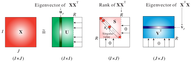
(b)

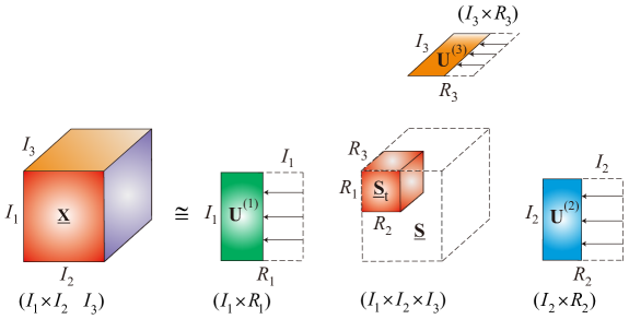
(c)

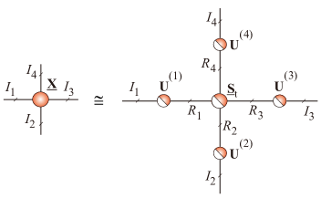
Figure 3.4: Graphical illustration of the truncated SVD and HOSVD. (a) The exact and truncated standard matrix SVD, ${\bf X}\cong{\bf U}{\bf S}{\bf V}^{\text{T}}$. (b) The truncated (approximative) HOSVD for a 3rd-order tensor calculated as $\underline{{\bf X}}\cong\underline{{\bf S}}_{t}\times_{1}{\bf U}^{(1)}\times_{2}{\bf U}^{(2)}\times_{3}{\bf U}^{(3)}$. (c) Tensor network notation for the HOSVD of a 4th-order tensor $\underline{{\bf X}}\cong\underline{{\bf S}}_{t}\times_{1}{\bf U}^{(1)}\times_{2}{\bf U}^{(2)}\times_{3}{\bf U}^{(3)}\times_{4}{\bf U}^{(4)}$. All the factor matrices, ${\bf U}^{(n)}\in\mathbb{R}^{I_{n}\times R_{n}}$, and the core tensor, $\underline{{\bf S}}_{t}=\underline{{\bf G}}\in\mathbb{R}^{R_{1}\times\cdots\times R_{N}}$, are orthogonal.

In practice, the orthogonal matrices ${\bf U}^{(n)}\in\mathbb{R}^{I_{n}\times R_{n}}$, with $R_{n}\leq I_{n}$, can be computed by applying both the randomized and standard truncated SVD to the unfolded mode-$n$ matrices, ${\bf X}_{(n)}\cong{\bf U}^{(n)}{\bf S}_{n}{\bf V}^{(n)\text{T}}\in\mathbb{R}^{I_{n}\times I_{1}\cdots I_{n-1}I_{n+1}\cdots I_{N}}$. After obtaining the orthogonal matrices ${\bf U}^{(n)}$ of left singular vectors of ${\bf X}_{(n)}$, for each $n$, the core tensor $\underline{{\bf G}}=\underline{{\bf S}}$ can be computed as

$$\underline{{\bf S}}=\underline{{\bf X}}\times_{1}{\bf U}^{(1)\;\text{T}}\times_{2}{\bf U}^{(2)\;\text{T}}\cdots\times_{N}{\bf U}^{(N)\;\text{T}},$$ (3.33)

so that

$$\underline{{\bf X}}=\underline{{\bf S}}\times_{1}{\bf U}^{(1)}\times_{2}{\bf U}^{(2)}\cdots\times_{N}{\bf U}^{(N)}.$$ (3.34)

Due to the orthogonality of the core tensor $\underline{{\bf S}}$, its slices are also mutually orthogonal.

Analogous to the standard truncated SVD, a large-scale data tensor, $\underline{{\bf X}}$, can be approximated by discarding the multilinear singular vectors and slices of the core tensor corresponding to small multilinear singular values. Figure 3.4 and Algorithm 2 outline the truncated HOSVD, for which any optimized matrix SVD procedure can be applied.

For large-scale tensors, the unfolding matrices, ${\bf X}_{(n)}\in\mathbb{R}^{I_{n}\times I_{\bar{n}}}$ ($I_{\bar{n}}=I_{1}\cdots I_{n}I_{n+1}\cdots I_{N}$) may become prohibitively large (with $I_{\bar{n}}\gg I_{n}$), easily exceeding the memory of standard computers. Using a direct and simple divide-and-conquer approach, the truncated SVD of an unfolding matrix, $\mathbf{X}_{(n)}={\bf U}^{(n)}{\bf S}_{n}{\bf V}^{(n)\text{T}}$, can be partitioned into $Q$ slices, as $\mathbf{X}_{(n)}=[\mathbf{X}_{1,n},\mathbf{X}_{2,n},\ldots,\mathbf{X}_{Q,n}]={\bf U}^{(n)}{\bf S}_{n}[\mathbf{V}_{1,n}^{\text{T}},\mathbf{V}_{2,n}^{\text{T}},\ldots,\mathbf{V}_{Q,n}^{\text{T}}]$. Next, the orthogonal matrices ${\bf U}^{(n)}$ and the diagonal matrices ${\bf S}_{n}$ can be obtained from the eigenvalue decompositions $\mathbf{X}_{(n)}\mathbf{X}_{(n)}^{\text{T}}={\bf U}^{(n)}{\bf S}_{n}^{2}{\bf U}^{(n)\text{T}}=\sum_{q}\mathbf{X}_{q,n}\mathbf{X}_{q,n}^{\text{T}}\in\mathbb{R}^{I_{n}\times I_{n}}$, allowing for the terms $\mathbf{V}_{q,n}=\mathbf{X}_{q,n}^{\text{T}}{\bf U}^{(n)}{\bf S}_{n}^{-1}$ to be computed separately. This enables us to optimize the size of the $q$th slice ${\bf X}_{q,n}\in\mathbb{R}^{I_{n}\times(I_{\bar{n}}/Q)}$ so as to match the available computer memory. Such a simple approach to compute matrices ${\bf U}^{(n)}$ and/or ${\bf V}^{(n)}$ does not require loading the entire unfolding matrices at once into computer memory; instead the access to the datasets is sequential. For current standard sizes of computer memory, the dimension $I_{n}$ is typically less than 10,000, while there is no limit on the dimension $I_{\bar{n}}=\prod_{k\neq n}I_{k}$.

For very large-scale and low-rank matrices, instead of the standard truncated SVD approach, we can alternatively apply the randomized SVD algorithm, which reduces the original data matrix ${\bf X}$ to a relatively small matrix by random sketching, i.e. through multiplication with a random sampling matrix $\Omega$ (see Algorithm 3). Note that we explicitly allow the rank of the data matrix ${\bf X}$ to be overestimated (that is, $\tilde{R}=R+P$, where $R$ is a true but unknown rank and $P$ is the over-sampling parameter) because it is easier to obtain more accurate approximation of this form. Performance of randomized SVD can be further improved by integrating multiple random sketches, that is, by multiplying a data matrix ${\bf X}$ by a set of random matrices $\mbox{\boldmath$\Omega$}_{p}$ for $p=1,2,\ldots,P$ and integrating leading low-dimensional subspaces by applying a Monte Carlo integration method [33].

Using special random sampling matrices, for instance, a sub-sampled random Fourier transform, substantial gain in the execution time can be achieved, together with the asymptotic complexity of ${\cal{O}}(IJ\log(R))$. Unfortunately, this approach is not accurate enough for matrices for which the singular values decay slowly [93].

0:  $N$th-order tensor $\underline{{\bf X}}\in\mathbb{R}^{I_{1}\times I_{2}\times\cdots\times I_{N}}$ and approximation accuracy $\varepsilon$ 0:  HOSVD in the Tucker format $\underline{\hat{\bf X}}=\llbracket\underline{{\bf S}};{\bf U}^{(1)},\ldots,\underline{{\bf U}}^{(N)}\rrbracket$, such that $\|\underline{{\bf X}}-\underline{\hat{\bf X}}\|_{F}\leq\varepsilon$ 1:  $\underline{{\bf S}}\leftarrow\underline{{\bf X}}$ 2:  for $n=1$ to $N$ do 3:     $[{\bf U}^{(n)},{\bf S},{\bf V}]=\textnormal{{truncated\_svd}}({\bf S}_{(n)},\frac{\varepsilon}{\sqrt{N}})$ 4:     $\underline{{\bf S}}\leftarrow{\bf V}{\bf S}$ 5:  end for 6:  $\underline{{\bf S}}\leftarrow\textnormal{{reshape}}(\underline{{\bf S}},[R_{1},\ldots,R_{N}])$ 7:  return  Core tensor $\underline{{\bf S}}$ and orthogonal factor matrices ${\bf U}^{(n)}\in\mathbb{R}^{I_{n}\times R_{n}}$.

Algorithm 2 Sequentially Truncated HOSVD [212]

0:  A matrix ${\bf X}\in\mathbb{R}^{I\times J}$, desired or estimated rank $R$, and oversampling parameter $P$ or overestimated rank $\widetilde{R}=R+P$, exponent of the power method $q$ ($q=0$ or $q=1$) 0:  An approximate rank-$\widetilde{R}$ SVD, ${\bf X}\cong{\bf U}{\bf S}{\bf V}^{\text{T}}$, i.e., orthogonal matrices ${\bf U}\in\mathbb{R}^{I\times\widetilde{R}}$, ${\bf V}\in\mathbb{R}^{J\times\widetilde{R}}$ and diagonal matrix of singular values ${\bf S}\in\mathbb{R}^{\widetilde{R}\times\widetilde{R}}$ 1:  Draw a random Gaussian matrix $\mbox{\boldmath$\Omega$}\in\mathbb{R}^{J\times\widetilde{R}}$, 2:  Form the sample matrix ${\bf Y}=({\bf X}{\bf X}^{\text{T}})^{q}\;{\bf X}\mbox{\boldmath$\Omega$}\in\mathbb{R}^{I\times\widetilde{R}}$ 3:  Compute a QR decomposition ${\bf Y}={\bf Q}{\bf R}$ 4:  Form the matrix ${\bf A}={\bf Q}^{\text{T}}{\bf X}\in\mathbb{R}^{\widetilde{R}\times J}$ 5:  Compute the SVD of the small matrix ${\bf A}$ as ${\bf A}=\widehat{\bf U}{\bf S}{\bf V}^{\text{T}}$ 6:  Form the matrix ${\bf U}={\bf Q}\widehat{\bf U}$.

Algorithm 3 Randomized SVD (rSVD) for large-scale and low-rank matrices with single sketch [93]

The truncated HOSVD can be optimized and implemented in several alternative ways. For example, if $R_{n}\ll I_{n}$, the truncated tensor $\underline{{\bf Z}}\leftarrow\underline{{\bf X}}\times_{1}{\bf U}^{(1)\text{T}}$ yields a smaller unfolding matrix ${\bf Z}_{(2)}\in\mathbb{R}^{I_{2}\times R_{1}I_{3}\cdots I_{N}}$, so that the multiplication ${\bf Z}_{(2)}{\bf Z}_{(2)}^{\text{T}}$ can be faster in the next iterations [212, 5].

Furthermore, since the unfolding matrices ${\bf Y}_{(n)}^{\text{T}}$ are typically very “tall and skinny”, a huge-scale truncated SVD and other constrained low-rank matrix factorizations can be computed efficiently based on the Hadoop / MapReduce paradigm [49, 48, 20].

Low multilinear rank approximation is always well-posed, however, in contrast to the standard truncated SVD for matrices, the truncated HOSVD does not yield the best multilinear rank approximation, but satisfies the quasi-best approximation property [59]

$$\|\underline{{\bf X}}-\llbracket\underline{{\bf S}};{\bf U}^{(1)},\ldots,{\bf U}^{(N)}\rrbracket\|\leq\sqrt{N}\|\underline{{\bf X}}-\underline{{\bf X}}_{\mbox{Best}}\|,$$ (3.35)

where $\underline{{\bf X}}_{\mbox{Best}}$ is the best multilinear rank approximation of $\underline{{\bf X}}$, for a specific tensor norm $\|\cdot\|$.

When it comes to the problem of finding the best approximation, the ALS type algorithm called the Higher Order Orthogonal Iteration (HOOI) exhibits both the advantages and drawbacks of ALS algorithms for CP decomposition. For the HOOI algorithms, see Algorithm 4 and Algorithm 5. For more sophisticated algorithms for Tucker decompositions with orthogonality and nonnegativity constraints, suitable for large-scale data tensors, see [169, 236, 49, 104].

Table 3.3: Basic multiway component analysis (MWCA)/Low-Rank Tensor Approximations (LRTA) and related multiway dimensionality reduction models. The symbol $\underline{{\bf X}}\in\mathbb{R}^{I_{1}\times I_{2}\times\cdots\times I_{N}}$ denotes a noisy data tensor, while ${\bf Y}=\underline{{\bf G}}\times_{1}{\bf B}^{(1)}\times_{2}{\bf B}^{(2)}\cdots\times_{N}{\bf B}^{(N)}$ is the general constrained Tucker model with the latent factor matrices ${\bf B}^{(n)}\in\mathbb{R}^{I_{n}\times R_{n}}$ and the core tensor $\underline{{\bf G}}\in\mathbb{R}^{R_{1}\times R_{2}\times\cdots\times R_{N}}$. In the special case of a CP decomposition, the core tensor is diagonal, $\underline{{\bf G}}=\underline{\mbox{\boldmath$\Lambda$}}\in\mathbb{R}^{R\times\cdots\times R}$, so that $\underline{{\bf Y}}=\sum_{r=1}^{R}\lambda_{r}({\bf b}_{r}^{(1)}\circ{\bf b}_{r}^{(2)}\circ\cdots\circ{\bf b}_{r}^{(N)})$.

Cost Function Constraints Multilinear (sparse) PCA (MPCA) $\max_{{\bf u}_{r}^{(n)}}\;\underline{{\bf X}}\bar{\times}_{1}{\bf u}_{r}^{(1)}\bar{\times}_{2}{\bf u}_{r}^{(2)}\cdots\bar{\times}_{N}{\bf u}_{r}^{(N)}+\gamma\sum_{n=1}^{N}\|{\bf u}_{r}^{(n)}\|_{1}$ ${\bf u}_{r}^{(n)\,\text{T}}\,{\bf u}_{r}^{(n)}=1,\;\forall(n,r)$ ${\bf u}_{r}^{(n)\,\text{T}}\,{\bf u}_{q}^{(n)}=0\;\;\mbox{for}\;\;r\neq q$ HOSVD/HOOI $\min_{{\bf U}^{(n)}}\;\|\underline{{\bf X}}-\underline{{\bf G}}\times_{1}{\bf U}^{(1)}\times_{2}{\bf U}^{(2)}\cdots\times_{N}{\bf U}^{(N)}\|_{F}^{2}$ ${\bf U}^{(n)\,\text{T}}\,{\bf U}^{(n)}={\bf I}_{R_{n}},\;\forall n$ Multilinear ICA $\min_{{\bf B}^{(n)}}\;\|\underline{{\bf X}}-\underline{{\bf G}}\times_{1}{\bf B}^{(1)}\times_{2}{\bf B}^{(2)}\cdots\times_{N}{\bf B}^{(N)}\|_{F}^{2}$ Vectors of ${\bf B}^{(n)}$ statistically as independent as possible Nonnegative CP/Tucker decomposition (NTF/NTD) [43] $\min_{{\bf B}^{(n)}}\;\|\underline{{\bf X}}-\underline{{\bf G}}\times_{1}{\bf B}^{(1)}\cdots\times_{N}{\bf B}^{(N)}\|_{F}^{2}$ $+\gamma\sum_{n=1}^{N}\sum_{r_{n}=1}^{R_{n}}\|{\bf b}^{(n)}_{r_{n}}\|_{1}$ Entries of $\underline{{\bf G}}$ and ${\bf B}^{(n)},\;\forall n$ are nonnegative Sparse CP/Tucker decomposition $\min_{{\bf B}^{(n)}}\;\|\underline{{\bf X}}-\underline{{\bf G}}\times_{1}{\bf B}^{(1)}\cdots\times_{N}{\bf B}^{(N)}\|_{F}^{2}$ $+\gamma\sum_{n=1}^{N}\sum_{r_{n}=1}^{R_{n}}\|{\bf b}^{(n)}_{r_{n}}\|_{1}$ Sparsity constraints imposed on ${\bf B}^{(n)}$ Smooth CP/Tucker decomposition (SmCP/SmTD) [228] $\min_{{\bf B}^{(n)}}\;\|\underline{{\bf X}}-\underline{\mbox{\boldmath$\Lambda$}}\times_{1}{\bf B}^{(1)}\cdots\times_{N}{\bf B}^{(N)}\|_{F}^{2}$ $+\gamma\sum_{n=1}^{N}\sum_{r=1}^{R}\|{\bf L}{\bf b}^{(n)}_{r}\|_{2}$ Smoothness imposed on vectors ${\bf b}_{r}^{(n)}$ of ${\bf B}^{(n)}\in\mathbb{R}^{I_{n}\times R}$,   $\forall n$ via a difference operator ${\bf L}$

0:  $N$th-order tensor $\underline{{\bf X}}\in\mathbb{R}^{I_{1}\times I_{2}\times\cdots\times I_{N}}$ (usually in Tucker/HOSVD format)

0:  Improved Tucker approximation using ALS approach, with orthogonal factor matrices ${\bf U}^{(n)}$

1:  Initialization via the standard HOSVD (see Algorithm 2)

2:  repeat

3:     for $n=1$ to $N$ do

4:        $\underline{{\bf Z}}\leftarrow\underline{{\bf X}}\times_{p\neq n}\{{\bf U}^{(p)\,\text{T}}\}$

5:        ${\bf C}\leftarrow{\bf Z}_{(n)}{\bf Z}_{(n)}^{\text{T}}\in\mathbb{R}^{R\times R}$

6:        ${\bf U}^{(n)}\leftarrow$ leading $R_{n}$ eigenvectors of ${\bf C}$

7:     end for

8:     $\underline{{\bf G}}\leftarrow\underline{{\bf Z}}\times_{N}{\bf U}^{(N)\,\text{T}}$

9:  until the cost function $(\|\underline{{\bf X}}\|^{2}_{F}-\|\underline{{\bf G}}\|^{2}_{F})$ ceases to decrease

10:  return  $\llbracket\underline{{\bf G}};{\bf U}^{(1)},{\bf U}^{(2)},\ldots,{\bf U}^{(N)}\rrbracket$

Algorithm 4 Higher Order Orthogonal Iteration (HOOI) [60, 5]

0:  $N$th-order tensor $\underline{{\bf X}}\in\mathbb{R}^{I_{1}\times I_{2}\times\cdots\times I_{N}}$ and multilinear rank $\{R_{1},R_{2},\ldots,R_{N}\}$

0:  Approximative representation of a tensor in Tucker format,

with orthogonal factor matrices ${\bf U}^{(n)}\in\mathbb{R}^{I_{n}\times R_{n}}$

1:  Initialize factor matrices ${\bf U}^{(n)}$ as random Gaussian matrices

Repeat steps (2)-(6) only two times:

2:  for $n=1$ to $N$ do

3:     $\underline{{\bf Z}}=\underline{{\bf X}}\times_{p\neq n}\{{\bf U}^{(p)\,\text{T}}\}$

4:     Compute $\tilde{\bf Z}^{(n)}={\bf Z}_{(n)}\mbox{\boldmath$\Omega$}^{(n)}\in\mathbb{R}^{I_{n}\times R_{n}}$, where $\mbox{\boldmath$\Omega$}^{(n)}\in\mathbb{R}^{\prod_{p\neq n}R_{p}\times R_{n}}$

is a random matrix drawn from Gaussian distribution

5:     Compute ${\bf U}^{(n)}$ as an orthonormal basis of $\tilde{\bf Z}^{(n)}$, e.g., by using QR decomposition

6:  end for

7:  Construct the core tensor as

$\underline{{\bf G}}=\underline{{\bf X}}\times_{1}{\bf U}^{(1)\;\text{T}}\times_{2}{\bf U}^{(2)\;\text{T}}\cdots\times_{N}{\bf U}^{(N)\;\text{T}}$

8:  return  $\underline{{\bf X}}\cong\llbracket\underline{{\bf G}};{\bf U}^{(1)},{\bf U}^{(2)},\ldots,\underline{{\bf U}}^{(N)}\rrbracket$

Algorithm 5 HOOI using randomization for large-scale data [238]

0:  $N$th-order tensor $\underline{{\bf X}}\in\mathbb{R}^{I_{1}\times I_{2}\times\cdots\times I_{N}}$, multilinear rank $\{R_{1},\ldots,R_{N}\}$ and desired constraints imposed on factor matrices ${\bf B}^{(n)}\in\mathbb{R}^{I_{n}\times R_{n}}$

0:  Tucker decomposition with constrained factor matrices ${\bf B}^{(n)}$

using LRMF and a simple unfolding approach

1:  Initialize randomly or via standard HOSVD (see Algorithm 2)

2:  for $n=1$ to $N$ do

3:     Compute specific LRMF or 2-way CA (e.g., RPCA, ICA, NMF) of unfolding ${\bf X}^{\text{T}}_{(n)}\cong{\bf A}^{(n)}{\bf B}^{(n)\;\text{T}}$ or ${\bf X}_{(n)}\cong{\bf B}^{(n)}{\bf A}^{(n)\;\text{T}}$

4:  end for

5:  Compute core tensor $\underline{{\bf G}}=\underline{{\bf X}}\times_{1}[{\bf B}^{(1)}]^{\dagger}\times_{2}[{\bf B}^{(2)}]^{\dagger}\cdots\times_{N}[{\bf B}^{(N)]^{\dagger}}$

6:  return  Constrained Tucker decomposition $\underline{{\bf X}}\cong\llbracket\underline{{\bf G}},{\bf B}^{(1)},\ldots,\underline{{\bf B}}^{(N)}\rrbracket$

Algorithm 6 Tucker decomposition with constrained factor matrices via 2-way CA /LRMF

When a data tensor $\underline{{\bf X}}$ is very large and cannot be stored in computer memory, another challenge is to compute a core tensor $\underline{{\bf G}}=\underline{{\bf S}}$ directly, using the formula (3.33). Such computation is performed sequentially by fast matrix-by-matrix multiplications, as illustrated in Figure 3.5(a) and (b).

We have shown that for very large-scale problems, it is useful to divide a data tensor $\underline{{\bf X}}$ into small blocks $\underline{{\bf X}}_{[k_{1},k_{2},\ldots,k_{N}]}$. In a similar way, we can partition the orthogonal factor matrices ${\bf U}^{(n)\text{T}}$ into the corresponding blocks of matrices ${\bf U}^{(n)\text{T}}_{[k_{n},p_{n}]}$, as illustrated in Figure 3.5(c) for 3rd-order tensors [221, 200]. For example, the blocks within the resulting tensor $\underline{{\bf G}}^{(n)}$ can be computed sequentially or in parallel, as follows:

$$\underline{{\bf G}}^{(n)}_{[k_{1},k_{2},\ldots,q_{n},\ldots,k_{N}]}=\sum_{k_{n}=1}^{K_{n}}{\bf X}_{[k_{1},k_{2},\ldots,k_{n},\ldots,k_{N}]}\times_{n}{\bf U}^{(n)\;\text{T}}_{[k_{n},q_{n}]}.$$ (3.36)

(a) Sequential computation

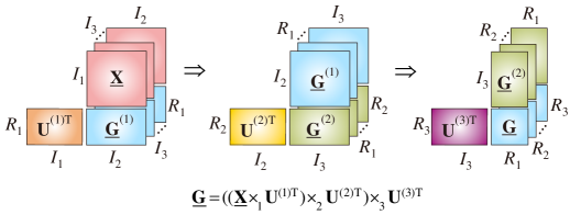
(b) Fast matrix-by-matrix approach

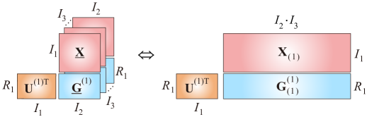
(c) Divide-and-conquer approach

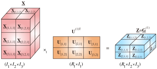
Figure 3.5: Computation of a multilinear (Tucker) product for large-scale HOSVD. (a) Standard sequential computing of multilinear products (TTM) $\underline{{\bf G}}=\underline{{\bf S}}=(((\underline{{\bf X}}\times_{1}{\bf U}^{(1)\text{T}})\times_{2}{\bf U}^{(2)\text{T}})\times_{3}{\bf U}^{(3)\text{T}})$. (b) Distributed implementation through fast matrix-by-matrix multiplications. (c) An alternative method for large-scale problems using the “divide and conquer” approach, whereby a data tensor, $\underline{{\bf X}}$, and factor matrices, ${\bf U}^{(n)\text{T}}$, are partitioned into suitable small blocks: Subtensors $\underline{{\bf X}}_{[k_{1},k_{2},k_{3}]}$ and block matrices ${\bf U}^{(1)\text{T}}_{[k_{1},p_{1}]}$. The blocks of a tensor, $\underline{{\bf Z}}=\underline{{\bf G}}^{(1)}=\underline{{\bf X}}\times_{1}{\bf U}^{(1)\text{T}}$, are computed as $\underline{{\bf Z}}_{[q_{1},k_{2},k_{3}]}=\sum_{k_{1}=1}^{K_{1}}{\bf X}_{[k_{1},k_{2},k_{3}]}\times_{1}{\bf U}^{(1)\text{T}}_{[k_{1},q_{1}]}$ (see Eq. (3.36) for a general case).

Applications. We have shown that the Tucker/HOSVD decomposition may be considered as a multilinear extension of PCA [124]; it therefore generalizes signal subspace techniques and finds application in areas including multilinear blind source separation, classification, feature extraction, and subspace-based harmonic retrieval [213, 90, 173, 137]. In this way, a low multilinear rank approximation achieved through Tucker decomposition may yield higher Signal-to-Noise Ratio (SNR) than the SNR for the original raw data tensor, which also makes Tucker decomposition a natural tool for signal compression and enhancement.

It was recently shown that HOSVD can also perform simultaneous subspace selection (data compression) and K-means clustering, both unsupervised learning tasks [99, 164]. This is important, as a combination of these methods can both identify and classify “relevant” data, and in this way not only reveal desired information but also simplify feature extraction.

Anomaly detection using HOSVD. Anomaly detection refers to the discrimination of some specific patterns, signals, outliers or features that do not conform to certain expected behaviors, trends or properties [32, 78]. While such analysis can be performed in different domains, it is most frequently based on spectral methods such as PCA, whereby high dimensional data are projected onto a lower-dimensional subspace in which the anomalies may be identified more easier. The main assumption within such approaches is that the normal and abnormal patterns, which may be difficult to distinguish in the original space, appear significantly different in the projected subspace. When considering very large datasets, since the basic Tucker decomposition model generalizes PCA and SVD, it offers a natural framework for anomaly detection via HOSVD, as illustrated in Figure 3.6. To handle the exceedingly large dimensionality, we may first compute tensor decompositions for sampled (pre-selected) small blocks of the original large-scale 3rd-order tensor, followed by the analysis of changes in specific factor matrices ${\bf U}^{(n)}$. A simpler form is straightforwardly obtained by fixing the core tensor and some factor matrices while monitoring the changes along one or more specific modes, as the block tensor moves from left to right as shown in Figure 3.6.

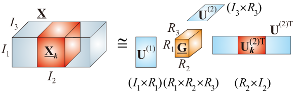
Figure 3.6: Conceptual model for performing the HOSVD for a very large-scale 3rd-order data tensor. This is achieved by dividing the tensor into blocks $\underline{{\bf X}}_{k}\cong\underline{{\bf G}}\times_{1}{\bf U}^{(1)}\times_{2}{\bf U}_{k}^{(2)}\times_{3}{\bf U}^{(3)}$, $(k=1,2\ldots,K)$. It assumed that the data tensor ${\bf X}\in\mathbb{R}^{I_{1}\times I_{2}\times I_{3}}$ is sampled by sliding the block $\underline{{\bf X}}_{k}$ from left to right (with an overlapping sliding window). The model can be used for anomaly detection by fixing the core tensor and some factor matrices while monitoring the changes along one or more specific modes (in our case mode two). Tensor decomposition is then first performed for a sampled (pre-selected) small block, followed by the analysis of changes in specific smaller–dimensional factor matrices ${\bf U}^{(n)}$.

3.5 Tensor Sketching Using Tucker Model

The notion of sketches refers to replacing the original huge matrix or tensor by a new matrix or tensor of a significantly smaller size or compactness, but which approximates well the original matrix/tensor. Finding such sketches in an efficient way is important for the analysis of big data, as a computer processor (and memory) is often incapable of handling the whole data-set in a feasible amount of time. For these reasons, the computation is often spread among a set of processors which for standard “all-in-one” SVD algorithms, are unfeasible.

Given a very large-scale tensor $\underline{{\bf X}}$ , a useful approach is to compute a sketch tensor $\underline{{\bf Z}}$ or set of sketch tensors $\underline{{\bf Z}}_{n}$ that are of significantly smaller sizes than the original one.

There exist several matrix and tensor sketching approaches: sparsification, random projections, fiber subset selections, iterative sketching techniques and distributed sketching. We review the main sketching approaches which are promising for tensors.

1. Sparsification generates a sparser version of the tensor which, in general, can be stored more efficiently and admit faster multiplications by factor matrices. This is achieved by decreasing the number on non-zero entries and quantizing or rounding up entries. A simple technique is element-wise sparsification which zeroes out all sufficiently small elements (below some threshold) of a data tensor, keeps all sufficiently large elements, and randomly samples the remaining elements of the tensor with sample probabilities proportional to the square of their magnitudes [152].

2. Random Projection based sketching randomly combines fibers of a data tensor in all or selected modes, and is related to the concept of a randomized subspace embedding, which is used to solve a variety of numerical linear algebra problems (see [208] and references therein).

3. Fiber subset selection, also called tensor cross approximation (TCA), finds a small subset of fibers which approximates the entire data tensor. For the matrix case, this problem is known as the Column/Row Subset Selection or CUR Problem which has been thoroughly investigated and for which there exist several algorithms with almost matching lower bounds [140, 64, 82].

3.6 Tensor Sketching via Multiple Random Projections

The random projection framework has been developed for computing structured low-rank approximations of a data tensor from (random) linear projections of much lower dimensions than the data tensor itself [28, 208]. Such techniques have many potential applications in large-scale numerical multilinear algebra and optimization problems.

(a)

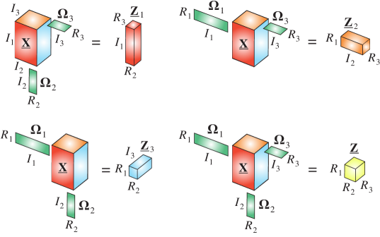
(b)

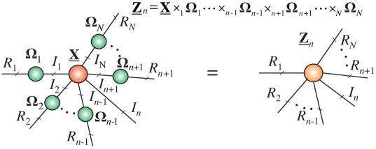
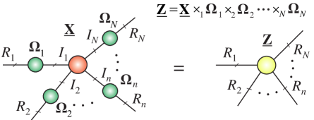
Figure 3.7: Illustration of tensor sketching using random projections of a data tensor. (a) Sketches of a 3rd-order tensor $\underline{{\bf X}}\in\mathbb{R}^{I_{1}\times I_{2}\times I_{3}}$ given by $\underline{{\bf Z}}_{1}=\underline{{\bf X}}\times_{2}\mbox{\boldmath$\Omega$}_{2}\times_{3}\mbox{\boldmath$\Omega$}_{3}\in\mathbb{R}^{I_{1}\times R_{2}\times R_{3}}$, $\underline{{\bf Z}}_{2}=\underline{{\bf X}}\times_{1}\mbox{\boldmath$\Omega$}_{1}\times_{3}\mbox{\boldmath$\Omega$}_{3}\in\mathbb{R}^{R_{1}\times I_{2}\times R_{3}}$, $\underline{{\bf Z}}_{3}=\underline{{\bf X}}\times_{1}\mbox{\boldmath$\Omega$}_{1}\times_{2}\mbox{\boldmath$\Omega$}_{2}\in\mathbb{R}^{R_{1}\times R_{2}\times I_{3}}$, and $\underline{{\bf Z}}=\underline{{\bf X}}\times_{1}\mbox{\boldmath$\Omega$}_{1}\times_{2}\mbox{\boldmath$\Omega$}_{2}\times_{3}\mbox{\boldmath$\Omega$}_{3}\in\mathbb{R}^{R_{1}\times R_{2}\times R_{3}}$. (b) Sketches for an $N$th-order tensor $\underline{{\bf X}}\in\mathbb{R}^{I_{1}\times\cdots\times I_{N}}$.

Notice that for an $N$th-order tensor $\underline{{\bf X}}\in\mathbb{R}^{I_{1}\times I_{2}\times\cdots\times I_{N}}$, we can compute the following sketches

$$\underline{{\bf Z}}=\underline{{\bf X}}\times_{1}\mbox{\boldmath$\Omega$}_{1}\times_{2}\mbox{\boldmath$\Omega$}_{2}\cdots\times_{N}\mbox{\boldmath$\Omega$}_{N}$$ (3.37)

and

$$\underline{{\bf Z}}_{\,n}=\underline{{\bf X}}\times_{1}\mbox{\boldmath$\Omega$}_{1}\cdots\times_{n-1}\mbox{\boldmath$\Omega$}_{n-1}\times_{n+1}\mbox{\boldmath$\Omega$}_{n+1}\cdots\times_{N}\mbox{\boldmath$\Omega$}_{N},$$ (3.38)

for $n=,1,2,\ldots,N$, where $\mbox{\boldmath$\Omega$}_{n}\in\mathbb{R}^{R_{n}\times I_{n}}$ are statistically independent random matrices with $R_{n}\ll I_{n}$, usually called test (or sensing) matrices.

A sketch can be implemented using test matrices drawn from various distributions. The choice of a distribution leads to some tradeoffs [208], especially regarding (i) the costs of randomization, computation, and communication to generate the test matrices; (ii) the storage costs for the test matrices and the sketch; (iii) the arithmetic costs for sketching and updates; (iv) the numerical stability of reconstruction algorithms; and (v) the quality of a priori error bounds. The most important distributions of random test matrices include:

• Gaussian random projections which generate random matrices with standard normal distribution. Such matrices usually provide excellent performance in practical scenarios and accurate a priori error bounds.

• Random matrices with orthonormal columns that span uniformly distributed random subspaces of dimensions $R_{n}$. Such matrices behave similar to Gaussian case, but usually exhibit even better numerical stability, especially when $R_{n}$ are large.

• Rademacher and super-sparse Rademacher random projections that have independent Rademacher entries which take the values $\pm 1$ with equal probability. Their properties are similar to standard normal test matrices, but exhibit some improvements in the cost of storage and computational complexity. In a special case, we may use ultra sparse Rademacher test matrices, whereby in each column of a test matrix independent Rademacher random variables are placed only in very few uniformly random locations determined by a sampling parameter $s$; the remaining entries are set to zero. In an extreme case of maximum sparsity, $s=1$, and each column of a test matrix has exactly only one nonzero entry.

• Subsampled randomized Fourier transforms based on test matrices take the following form

  $$\mbox{\boldmath$\Omega$}_{n}={\bf P}_{n}{\bf F}_{n}{\bf D}_{n},$$ (3.39)

  where ${\bf D}_{n}$ are diagonal square matrices with independent Rademacher entries, ${\bf F}_{n}$ are discrete cosine transform (DCT) or discrete Fourier transform (DFT) matrices, and entries of the matrix ${\bf P}_{n}$ are drawn at random from a uniform distribution.

Example. The concept of tensor sketching via random projections is illustrated in Figure 3.7 for a 3rd-order tensor and for a general case of $N$th-order tensors. For a 3rd-order tensor with volume (number of entries) $I_{1}I_{2}I_{3}$ we have four possible sketches which are subtensors of much smaller sizes, e.g., $I_{1}R_{2}R_{3}$, with $R_{n}\ll I_{n}$, if the sketching is performed along mode-2 and mode-3, or $R_{1}R_{2}R_{3}$, if the sketching is performed along all three modes (Figure 3.7(a) bottom right). From these subtensors we can reconstruct any huge tensor if it has low a multilinear rank (lower than $\{R_{1},R_{2},\ldots,R_{n}\}$).

In more general scenario, it can be shown [28] that the $N$th order tensor data tensor $\underline{{\bf X}}$ with sufficiently low-multilinear rank can be reconstructed perfectly from the sketch tensors $\underline{{\bf Z}}_{n}$, for $n=1,2,\ldots,N$, as follows

$$\underline{\hat{{\bf X}}}=\underline{{\bf Z}}\times_{1}{\bf B}^{(1)}\times_{2}{\bf B}^{(2)}\cdots\times_{N}{\bf B}^{(N)},$$ (3.40)

where ${\bf B}^{(n)}=[\underline{{\bf Z}}_{n}]_{(n)}{\bf Z}_{(n)}^{{\dagger}}$ for $n=1,2,\ldots,N$ (for more detail see the next section).

3.7 Matrix/Tensor Cross-Approximation (MCA/TCA)

Huge-scale matrices can be factorized using the Matrix Cross-Approximation (MCA) method, which is also known under the names of Pseudo-Skeleton or CUR matrix decompositions [85, 84, 142, 141, 162, 16, 17, 116]. The main idea behind the MCA is to provide reduced dimensionality of data through a linear combination of only a few “meaningful” components, which are exact replicas of columns and rows of the original data matrix. Such an approach is based on the fundamental assumption that large datasets are highly redundant and can therefore be approximated by low-rank matrices, which significantly reduces computational complexity at the cost of a marginal loss of information.

The MCA method factorizes a data matrix ${\bf X}\in\mathbb{R}^{I\times J}$ as [84, 85] (see Figure 3.8)

$${\bf X}={\bf C}{\bf U}{\bf R}+{\bf E},$$ (3.41)

where ${\bf C}\in\mathbb{R}^{I\times C}$ is a matrix constructed from $C$ suitably selected columns of the data matrix ${\bf X}$, matrix ${\bf R}\in\mathbb{R}^{R\times J}$ consists of $R$ appropriately selected rows of ${\bf X}$, and matrix ${\bf U}\in\mathbb{R}^{C\times R}$ is calculated so as to minimize the norm of the error ${\bf E}\in\mathbb{R}^{I\times J}$.

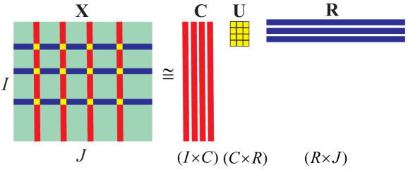
Figure 3.8: Principle of the matrix cross-approximation which decomposes a huge matrix ${\bf X}$ into a product of three matrices, whereby only a small-size core matrix ${\bf U}$ needs to be computed.

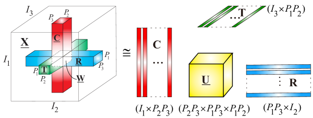
Figure 3.9: The principle of the tensor cross-approximation (TCA) algorithm, illustrated for a large-scale 3rd-order tensor $\underline{{\bf X}}\cong\underline{{\bf U}}\times_{1}{\bf C}\times_{2}{\bf R}\times_{3}{\bf T}=\llbracket\underline{{\bf U}};{\bf C},{\bf R},{\bf T}\rrbracket$, where $\underline{{\bf U}}=\underline{{\bf W}}\times_{1}\mathbf{W}_{(1)}^{\dagger}\times_{2}\mathbf{W}_{(2)}^{\dagger}\times_{3}\mathbf{W}_{(3)}^{\dagger}=\llbracket\underline{{\bf W}};\mathbf{W}_{(1)}^{\dagger},\mathbf{W}_{(2)}^{\dagger},\mathbf{W}_{(3)}^{\dagger}\rrbracket\in\mathbb{R}^{P_{2}P_{3}\times P_{1}P_{3}\times P_{1}P_{2}}$ and $\underline{{\bf W}}\in\mathbb{R}^{P_{1}\times P_{2}\times P_{3}}$. For simplicity of illustration, we assume that the selected fibers are permuted, so as to become clustered as subtensors, $\underline{{\bf C}}\in\mathbb{R}^{I_{1}\times P_{2}\times P_{3}}$, $\underline{{\bf R}}\in\mathbb{R}^{P_{1}\times I_{2}\times P_{3}}$ and $\underline{{\bf T}}\in\mathbb{R}^{P_{1}\times P_{2}\times I_{3}}$.

(a)

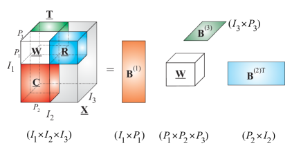
(b)

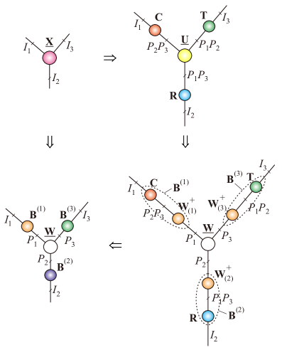
Figure 3.10: The Tucker decomposition of a low multilinear rank 3rd-order tensor using the cross-approximation approach. (a) Standard block diagram. (b) Transformation from the TCA in the Tucker format, ${\bf X}\cong\underline{{\bf U}}\times_{1}{\bf C}\times_{2}{\bf R}\times_{3}{\bf T}$, into a standard Tucker representation, $\underline{{\bf X}}\cong\underline{{\bf W}}\times_{1}{\bf B}^{(1)}\times_{2}{\bf B}^{(2)}\times_{3}{\bf B}^{(3)}=\llbracket\underline{{\bf W}};{\bf C}{\bf W}_{(1)}^{\dagger},{\bf R}{\bf W}_{(2)}^{\dagger},{\bf T}{\bf W}_{(3)}^{\dagger}\rrbracket$, with a prescribed core tensor $\underline{{\bf W}}$.

A simple modification of this formula, whereby the matrix ${\bf U}$ is absorbed into either ${\bf C}$ or ${\bf R}$, yields the so-called CR matrix factorization or Column/Row Subset selection:

$${\bf X}\cong{\bf C}\tilde{\bf R}=\tilde{\bf C}{\bf R}$$ (3.42)

for which the bases can be either the columns, ${\bf C}$, or rows, ${\bf R}$, while $\tilde{\bf R}={\bf U}{\bf R}$ and $\tilde{\bf C}={\bf C}{\bf U}$.

For dimensionality reduction, $C\ll J$ and $R\ll I$, and the columns and rows of ${\bf X}$ should be chosen optimally, in the sense of providing a high “statistical leverage” and the best low-rank fit to the data matrix, while at the same time minimizing the cost function $\|{\bf E}\|_{F}^{2}$. For a given set of columns, ${\bf C}$, and rows, ${\bf R}$, the optimal choice for the core matrix is ${\bf U}={\bf C}^{\dagger}{\bf X}({\bf R}^{\dagger})^{\text{T}}$. This requires access to all the entries of ${\bf X}$ and is not practical or feasible for large-scale data. In such cases, a pragmatic choice for the core matrix would be ${\bf U}={\bf W}^{\dagger}$, where the matrix ${\bf W}\in\mathbb{R}^{R\times C}$ is composed from the intersections of the selected rows and columns. It should be noted that for rank$({\bf X})\leq\min\{C,R\}$ the cross-approximation is exact. For the general case, it has been proven that when the intersection submatrix ${\bf W}$ is of maximum volume, the matrix cross-approximation is close to the optimal SVD solution. The problem of finding a submatrix with maximum volume has exponential complexity, however, suboptimal matrices can be found using fast greedy algorithms [222, 144, 179, 4].

The concept of MCA can be generalized to tensor cross-approximation (TCA) (see Figure 3.9) through several approaches, including:

• Applying the MCA decomposition to a matricized version of the tensor data [142];

• Operating directly on fibers of a data tensor which admits a low-rank Tucker approximation, an approach termed the Fiber Sampling Tucker Decomposition (FSTD) [26, 27, 28].

Real-life structured data often admit good low-multilinear rank approximations, and the FSTD provides such a low-rank Tucker decomposition which is practical as it is directly expressed in terms of a relatively small number of fibers of the data tensor.

For example, for a 3rd-order tensor, $\underline{{\bf X}}\in\mathbb{R}^{I_{1}\times I_{2}\times I_{3}}$, for which an exact rank-$(R_{1},R_{2},R_{3})$ Tucker representation exists, the FSTD selects $P_{n}\geq R_{n}$, $n=1,2,3$, indices in each mode; this determines an intersection subtensor, $\underline{{\bf W}}\in\mathbb{R}^{P_{1}\times P_{2}\times P_{3}}$, so that the following exact Tucker representation can be obtained (see Figure 3.10)

$$\underline{{\bf X}}=\llbracket\underline{{\bf U}};{\bf C},{\bf R},{\bf T}\rrbracket,$$ (3.43)

where the core tensor is computed as $\underline{{\bf U}}=\underline{{\bf G}}=\llbracket\underline{{\bf W}};\mathbf{W}_{(1)}^{\dagger},\mathbf{W}_{(2)}^{\dagger},\mathbf{W}_{(3)}^{\dagger}\rrbracket$, while the factor matrices, ${\bf C}\in\mathbb{R}^{I_{1}\times P_{2}P_{3}},{\bf R}\in\mathbb{R}^{I_{2}\times P_{1}P_{3}},{\bf T}\in\mathbb{R}^{I_{3}\times P_{1}P_{2}}$, contain the fibers which are the respective subsets of the columns $\underline{{\bf C}}$, rows $\underline{{\bf R}}$ and tubes $\underline{{\bf T}}$. An equivalent Tucker representation is then given by

$$\underline{{\bf X}}=\llbracket\underline{{\bf W}};\mathbf{C}\mathbf{W}_{(1)}^{\dagger},\mathbf{R}\mathbf{W}_{(2)}^{\dagger},\mathbf{T}\mathbf{W}_{(3)}^{\dagger}\rrbracket.$$ (3.44)

Observe that for $N=2$, the TCA model simplifies into the MCA for a matrix case, ${\bf X}={\bf C}{\bf U}{\bf R}$, for which the core matrix is $\mathbf{U}=\llbracket\mathbf{W};\mathbf{W}_{(1)}^{\dagger},\mathbf{W}_{(2)}^{\dagger}\rrbracket=\mathbf{W}^{\dagger}\mathbf{W}\mathbf{W}^{\dagger}=\mathbf{W}^{\dagger}$.

For a general case of an $N$th-order tensor, we can show [26] that a tensor, $\underline{{\bf X}}\in\mathbb{R}^{I_{1}\times I_{2}\times\cdots\times I_{N}}$, with a low multilinear rank $\{R_{1},R_{2},\ldots,R_{N}\}$, where $R_{n}\leq I_{n},\,\forall n$, can be fully reconstructed via the TCA FSTD, $\underline{{\bf X}}=\llbracket\underline{{\bf U}};{\bf C}^{(1)},{\bf C}^{(2)},\ldots,{\bf C}^{(N)}\rrbracket$, using only $N$ factor matrices ${\bf C}^{(n)}\in\mathbb{R}^{I_{n}\times P_{n}}$ $(n=1,2,\ldots,N)$, built up from the fibers of the data and core tensors, $\underline{{\bf U}}=\underline{{\bf G}}=\llbracket\underline{{\bf W}};\mathbf{W}_{(1)}^{\dagger},\mathbf{W}_{(2)}^{\dagger},\ldots,\mathbf{W}_{(N)}^{\dagger}\rrbracket$, under the condition that the subtensor $\underline{{\bf W}}\in\mathbb{R}^{P_{1}\times P_{2}\times\cdots\times P_{N}}$ with $P_{n}\geq R_{n},\;\forall n$, has the multilinear rank $\{R_{1},R_{2},\ldots,R_{N}\}$.

The selection of a minimum number of suitable fibers depends upon a chosen optimization criterion. A strategy which requires access to only a small subset of entries of a data tensor, achieved by selecting the entries with maximum modulus within each single fiber, is given in [26]. These entries are selected sequentially using a deflation approach, thus making the tensor cross-approximation FSTD algorithm suitable for the approximation of very large-scale but relatively low-order tensors (including tensors with missing fibers or entries).

It should be noted that an alternative efficient way to estimate subtensors $\underline{{\bf W}},\underline{{\bf C}},\underline{{\bf R}}$ and $\underline{{\bf T}}$ is to apply random projections as follows

$$\underline{{\bf W}} = \underline{{\bf Z}}=\underline{{\bf X}}\times_{1}\mbox{\boldmath$\Omega$}_{1}\times_{2}\mbox{\boldmath$\Omega$}_{2}\times_{3}\mbox{\boldmath$\Omega$}_{3}\in\mathbb{R}^{P_{1}\times P_{2}\times P_{3}},$$

$$\underline{{\bf C}} = \underline{{\bf Z}}_{1}=\underline{{\bf X}}\times_{2}\mbox{\boldmath$\Omega$}_{2}\times_{3}\mbox{\boldmath$\Omega$}_{3}\in\mathbb{R}^{I_{1}\times P_{2}\times P_{3}},$$

$$\underline{{\bf R}} = \underline{{\bf Z}}_{2}=\underline{{\bf X}}\times_{1}\mbox{\boldmath$\Omega$}_{1}\times_{3}\mbox{\boldmath$\Omega$}_{3}\in\mathbb{R}^{P_{1}\times I_{2}\times P_{3}},$$

$$\underline{{\bf T}} = \underline{{\bf Z}}_{3}=\underline{{\bf X}}\times_{1}\mbox{\boldmath$\Omega$}_{1}\times_{2}\mbox{\boldmath$\Omega$}_{2}\in\mathbb{R}^{P_{1}\times P_{2}\times I_{3}},$$ (3.45)

where $\mbox{\boldmath$\Omega$}_{n}\in\mathbb{R}^{P_{n}\times I_{n}}$ with $P_{n}\geq R_{n}$ for $n=1,2,3$ are independent random matrices. We explicitly assume that the multilinear rank $\{P_{1},P_{2},\ldots,P_{N}\}$ of approximated tensor to be somewhat larger than a true multilinear rank $\{R_{1},R_{2},\ldots,R_{N}\}$ of target tensor, because it is easier to obtain an accurate approximation in this form.

3.8 Multiway Component Analysis (MWCA)

3.8.1 Multilinear Component Analysis Using Constrained Tucker Decomposition

The great success of 2-way component analyses (PCA, ICA, NMF, SCA) is largely due to the existence of very efficient algorithms for their computation and the possibility to extract components with a desired physical meaning, provided by the various flexible constraints exploited in these methods. Without these constraints, matrix factorizations would be less useful in practice, as the components would have only mathematical but not physical meaning.

Similarly, to exploit the full potential of tensor factorization/decompositions, it is a prerequisite to impose suitable constraints on the desired components. In fact, there is much more flexibility for tensors, since different constraints can be imposed on the matrix factorizations in every mode $n$ a matricized tensor ${\bf X}_{(n)}$ (see Algorithm 6 and Figure 3.11).

Such physically meaningful representation through flexible mode-wise constraints underpins the concept of multiway component analysis (MWCA). The Tucker representation of MWCA naturally accommodates such diversities in different modes. Besides the orthogonality, alternative constraints in the Tucker format include statistical independence, sparsity, smoothness and nonnegativity [213, 43, 235, 42] (see Table 3.3).

The multiway component analysis (MWCA) based on the Tucker-$N$ model can be computed directly in two or three steps:

1. For each mode $n$ $(n=1,2,\ldots,N)$ perform model reduction and matricization of data tensors sequentially, then apply a suitable set of 2-way CA/BSS algorithms to the so reduced unfolding matrices, $\tilde{\bf X}_{(n)}$. In each mode, we can apply different constraints and a different 2-way CA algorithms.

2. Compute the core tensor using, e.g., the inversion formula, $\hat{\underline{{\bf G}}}=\underline{{\bf X}}\times_{1}\mathbf{B}^{(1)}{}^{\dagger}\times_{2}\mathbf{B}^{(2)}{}^{\dagger}\cdots\times_{N}\mathbf{B}^{(N)}{}^{\dagger}$. This step is quite important because core tensors often model the complex links among the multiple components in different modes.

3. Optionally, perform fine tuning of factor matrices and the core tensor by the ALS minimization of a suitable cost function, e.g., $\|\underline{{\bf X}}-\llbracket\underline{{\bf G}};{\bf B}^{(1)},\ldots,{\bf B}^{(N)}\rrbracket\|^{2}_{F}$, subject to specific imposed constraints.

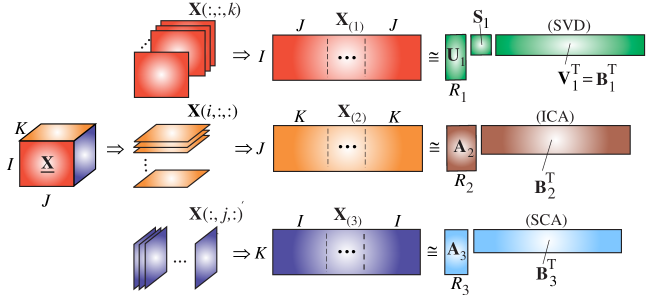
Figure 3.11: Multiway Component Analysis (MWCA) for a third-order tensor via constrained matrix factorizations, assuming that the components are: orthogonal in the first mode, statistically independent in the second mode and sparse in the third mode.

3.9 Analysis of Coupled Multi-block Matrix/Tensors – Linked Multiway Component Analysis (LMWCA)

We have shown that TDs provide natural extensions of blind source separation (BSS) and 2-way (matrix) Component Analysis to multi-way component analysis (MWCA) methods.

In addition, TDs are suitable for the coupled multiway analysis of multi-block datasets, possibly with missing values and corrupted by noise. To illustrate the simplest scenario for multi-block analysis, consider the block matrices, ${\bf X}^{(k)}\in\mathbb{R}^{I\times J}$, which need to be approximately jointly factorized as

$${\bf X}^{(k)}\cong{\bf A}{\bf G}^{(k)}{\bf B}^{\text{T}},\quad(k=1,2,\ldots,K),$$ (3.46)

where ${\bf A}\in\mathbb{R}^{I\times R_{1}}$ and ${\bf B}\in\mathbb{R}^{J\times R_{2}}$ are common factor matrices and ${\bf G}^{(k)}\in\mathbb{R}^{R_{1}\times R_{2}}$ are reduced-size matrices, while the number of data matrices $K$ can be huge (hundreds of millions or more matrices). Such a simple model is referred to as the Population Value Decomposition (PVD) [51]. Note that the PVD is equivalent to the unconstrained or constrained Tucker-2 model, as illustrated in Figure 3.12. In a special case with square diagonal matrices, ${\bf G}^{(k)}$, the model is equivalent to the CP decomposition and is related to joint matrix diagonalization [56, 203, 31]. Furthermore, if ${\bf A}={\bf B}$ then the PVD model is equivalent to the RESCAL model [153].

Observe that the PVD/Tucker-2 model is quite general and flexible, since any high-order tensor, $\underline{{\bf X}}\in\mathbb{R}^{I_{1}\times I_{2}\times\cdots\times I_{N}}$ (with $N>3$), can be reshaped and optionally permuted into a “skinny and tall” 3rd-order tensor, $\underline{\widetilde{\bf X}}\in\mathbb{R}^{J\;\times\;J\;\times\;K}$, with e.g., $I=I_{1},\;J=I_{2}$ and $K=I_{3}I_{4}\cdots I_{N}$, for which PVD/Tucker-2 Algorithm 8 can be applied.

As previously mentioned, various constraints, including sparsity, nonnegativity or smoothness can be imposed on the factor matrices, ${\bf A}$ and ${\bf B}$, to obtain physically meaningful and unique components.

(a)

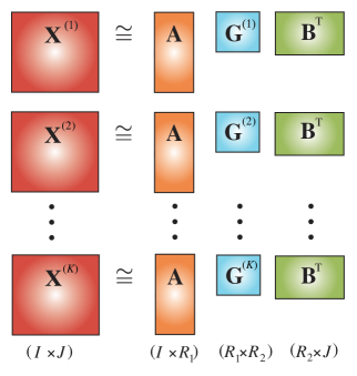
(b)

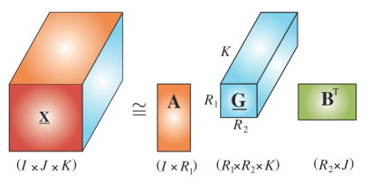
Figure 3.12: Concept of the Population Value Decomposition (PVD). (a) Principle of simultaneous multi-block matrix factorizations. (b) Equivalent representation of the PVD as the constrained or unconstrained Tucker-2 decomposition, $\underline{{\bf X}}\cong\underline{{\bf G}}\times_{1}{\bf A}\times_{2}{\bf B}$. The objective is to find the common factor matrices, ${\bf A}$, ${\bf B}$ and the core tensor, $\underline{{\bf G}}\in\mathbb{R}^{R_{1}\times R_{2}\times K}$.

0:  A set of matrices ${\bf X}_{k}\in\mathbb{R}^{I\times J}$, for $k=1,\ldots,K$ (typically, $\;K\gg\max\{I,J\}$) 0:  Factor matrices ${\bf A}\in\mathbb{R}^{I\times R_{1}}$, ${\bf B}\in\mathbb{R}^{J\times R_{2}}$ and ${\bf G}_{k}\in\mathbb{R}^{R_{1}\times R_{2}}$, with orthogonality constraints ${\bf A}^{\text{T}}{\bf A}={\bf I}_{R_{1}}$ and ${\bf B}^{\text{T}}{\bf B}={\bf I}_{R_{2}}$ 1:  for $k=1$ to $K$ do 2:     Perform truncated SVD, ${\bf X}_{k}={\bf U}_{k}{\bf S}_{k}{\bf V}_{k}^{\text{T}}$, using $R$ largest singular values 3:  end for 4:  Construct short and wide matrices: ${\bf U}=[{\bf U}_{1}{\bf S}_{1},\ldots,{\bf U}_{K}{\bf S}_{K}]\in\mathbb{R}^{I\times KR}$ and ${\bf V}=[{\bf V}_{1}{\bf S}_{1},\ldots,{\bf V}_{K}{\bf S}_{K}]\in\mathbb{R}^{J\times KR}$ 5:  Perform SVD (or QR) for the matrices ${\bf U}$ and ${\bf V}$ Obtain common orthogonal matrices ${\bf A}$ and ${\bf B}$ as left-singular matrices of ${\bf U}$ and ${\bf V}$, respectively 6:  for $k=1$ to $K$ do 7:     Compute ${\bf G}_{k}={\bf A}^{\text{T}}{\bf X}_{k}{\bf B}$ 8:  end for

Algorithm 7 Population Value Decomposition (PVD) with orthogonality constraints

0:  A 3rd-order tensor $\underline{{\bf X}}\in\mathbb{R}^{I\times J\times K}$ (typically, $K\gg\max\{I,J\}$) and estimation accuracy $\varepsilon$ 0:  A set of orthogonal matrices ${\bf A}\in\mathbb{R}^{I\times R_{1}}$, ${\bf B}\in\mathbb{R}^{J\times R_{2}}$ and core tensor $\underline{{\bf G}}\in\mathbb{R}^{R_{1}\times R_{2}\times K}$, which satisfies the constraint $\|\underline{{\bf X}}-\underline{{\bf G}}\times_{1}{\bf A}\times{\bf B}\|_{F}^{2}\leq\varepsilon^{2}$ , s.t, ${\bf A}^{\text{T}}{\bf A}={\bf I}_{R_{1}}$ and ${\bf B}^{\text{T}}{\bf B}={\bf I}_{R_{2}}$. 1:  Initialize ${\bf A}={\bf I}_{I}\in\mathbb{R}^{I\times I}$, $R_{1}=I$ 2:  while not converged or iteration limit is not reached do 3:     Compute the tensor $\underline{{\bf Z}}^{(1)}=\underline{{\bf X}}\times_{1}{\bf A}^{\text{T}}\in\mathbb{R}^{R_{1}\times J\times K}$ 4:     Compute EVD of a small matrix ${\bf Q}_{1}={\bf Z}_{(2)}^{(1)}{\bf Z}_{(2)}^{(1)\;\text{T}}\in\mathbb{R}^{J\times J}$ as ${\bf Q}_{1}={\bf B}\;\mathop{\rm diag}\nolimits\left(\lambda_{1},\cdots,\lambda_{R_{2}}\right)\;{\bf B}^{\text{T}}$, such that $\sum_{r_{2}=1}^{R_{2}}\lambda_{r_{2}}\geq\|\underline{{\bf X}}\|_{F}^{2}-\varepsilon^{2}\geq\sum_{r_{2}=1}^{R_{2}-1}\lambda_{r_{2}}$ 5:     Compute tensor $\underline{{\bf Z}}^{(2)}=\underline{{\bf X}}\times_{2}{\bf B}^{\text{T}}\in\mathbb{R}^{I\times R_{2}\times K}$ 6:     Compute EVD of a small matrix ${\bf Q}_{2}={\bf Z}_{(1)}^{(2)}{\bf Z}_{(1)}^{(2)\;\text{T}}\in\mathbb{R}^{I\times I}$ as ${\bf Q}_{2}={\bf A}\;\mathop{\rm diag}\nolimits\left(\lambda_{1},\ldots,\lambda_{R_{1}}\right)\;{\bf A}^{\text{T}}$, such that $\sum_{r_{1}=1}^{R_{1}}\lambda_{r_{1}}\geq\|\underline{{\bf X}}\|_{F}^{2}-\varepsilon^{2}\geq\sum_{r_{1}=1}^{R_{1}-1}\lambda_{r_{1}}$ 7:  end while 8:  Compute the core tensor $\underline{{\bf G}}=\underline{{\bf X}}\times_{1}{\bf A}^{\text{T}}\times_{2}{\bf B}^{\text{T}}$ 9:  return  ${\bf A},{\bf B}$ and $\underline{{\bf G}}$.

Algorithm 8 Orthogonal Tucker-2 decomposition with a prescribed approximation accuracy [170]

A simple SVD/QR based algorithm for the PVD with orthogonality constraints is presented in Algorithm 7 [51, 49, 219]. However, it should be noted that this algorithm does not provide an optimal solution in the sense of the absolute minimum of the cost function, $\sum_{k=1}^{K}\|{\bf X}_{k}-{\bf A}{\bf G}_{k}{\bf B}^{\text{T}}\|_{F}^{2}$, and for data corrupted by Gaussian noise, better performance can be achieved using the HOOI-2 given in Algorithm 4, for $N=3$. An improved PVD algorithm referred to as Tucker-2 algorithm is given in Algorithm 8 [170].

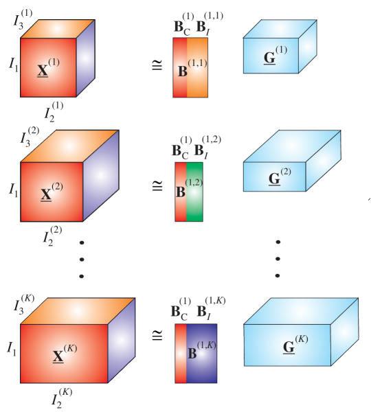
Figure 3.13: Linked Multiway Component Analysis (LMWCA) for coupled 3rd-order data tensors $\underline{{\bf X}}^{(1)},\ldots,\underline{{\bf X}}^{(K)}$; these can have different dimensions in every mode, except for the mode-1 for which the size is $I_{1}$ for all $\underline{{\bf X}}^{(k)}$. Linked Tucker-1 decompositions are then performed in the form $\underline{{\bf X}}^{(k)}\cong\underline{{\bf G}}^{(k)}\times_{1}{\bf B}^{(1,k)}$, where partially correlated factor matrices are ${\bf B}^{(1,k)}=[{\bf B}^{(1)}_{C},{\bf B}^{(1,k)}_{I}]\in\mathbb{R}^{I_{1}\times R_{k}}$, $(k=1,2,\ldots,K)$. The objective is to find the common components, ${\bf B}^{(1)}_{C}\in\mathbb{R}^{I_{1}\times C}$, and individual components, ${\bf B}^{(1,k)}_{I}\in\mathbb{R}^{I_{1}\times(R_{k}-C)}$, where $C\leq\min\{R_{1},\ldots,R_{K}\}$ is the number of common components in mode-1.

Linked MWCA. Consider the analysis of multi-modal high-dimensional data collected under the same or very similar conditions, for example, a set of EEG and MEG or EEG and fMRI signals recorded for different subjects over many trials and under the same experimental configurations and mental tasks. Such data share some common latent (hidden) components but can also have their own independent features. As a result, it is advantageous and natural to analyze such data in a linked way instead of treating them independently. In such a scenario, the PVD model can be generalized to multi-block matrix/tensor datasets [38, 237, 239].

(a)

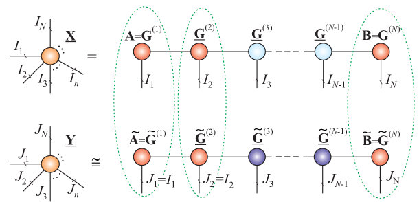
(b)

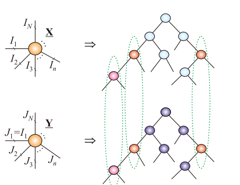
Figure 3.14: Conceptual models of generalized Linked Multiway Component Analysis (LMWCA) applied to the cores of high-order TNs. The objective is to find a suitable tensor decomposition which yields the maximum number of cores that are as much correlated as possible. (a) Linked Tensor Train (TT) networks. (b) Linked Hierarchical Tucker (HT) networks with the correlated cores indicated by ellipses in broken lines.

The linked multiway component analysis (LMWCA) for multi-block tensor data can therefore be formulated as a set of approximate simultaneous (joint) Tucker-$(1,N)$ decompositions of a set of data tensors, $\underline{{\bf X}}^{(k)}\in\mathbb{R}^{I_{1}^{(k)}\times I_{2}^{(k)}\times\cdots\times I_{N}^{(k)}}$, with $I_{1}^{(k)}=I_{1}$ for $k=1,2,\ldots,K$, in the form (see Figure 3.13)

$$\underline{{\bf X}}^{(k)}=\underline{{\bf G}}^{(k)}\times_{1}{\bf B}^{(1,k)},\quad(k=1,2,\ldots K)$$ (3.47)

where each factor (component) matrix, ${\bf B}^{(1,k)}=[{\bf B}^{(1)}_{C},\;{\bf B}^{(1,k)}_{I}]\in\mathbb{R}^{I_{1}\times R_{k}}$, comprises two sets of components: (1) Components ${\bf B}^{(1)}_{C}\in\mathbb{R}^{I_{1}\times C}$ (with $0\leq C\leq R_{k}$), $\;\forall k$, which are common for all the available blocks and correspond to identical or maximally correlated components, and (2) components ${\bf B}^{(1,k)}_{I}\in\mathbb{R}^{I_{1}\times(R_{k}-C)}$, which are different independent processes for each block, $k$, these can be, for example, latent variables independent of excitations or stimuli/tasks. The objective is therefore to estimate the common (strongly correlated) components, ${\bf B}_{C}^{(1)}$, and statistically independent (individual) components, ${\bf B}^{(1,k)}_{I}$ [38].

If ${\bf B}^{(n,k)}={\bf B}^{(n)}_{C}\in\mathbb{R}^{I_{n}\times R_{n}}$ for a specific mode $n$ (in our case $n=1$), and under the additional assumption that the block tensors are of the same order and size, the problem simplifies into generalized Common Component Analysis or tensor Population Value Decomposition (PVD) and can be solved by concatenating all data tensors along one mode, followed by constrained Tucker or CP decompositions [173].

In a more general scenario, when $C_{n}<R_{n}$, we can unfold each data tensor $\underline{{\bf X}}^{(k)}$ in the common mode, and perform a set of simultaneous matrix factorizations, e.g., ${\bf X}_{(1)}^{(k)}\cong{\bf B}^{(1)}_{C}\mathbf{A}^{(1,k)}_{C}+\mathbf{B}^{(1,k)}_{I}\mathbf{A}^{(1,k)}_{I}$, through solving the constrained optimization problems

$$\begin{split}\min\;&\sum_{k=1}^{K}\|{\bf X}_{(1)}^{(k)}-{\bf B}^{(1)}_{C}\mathbf{A}^{(1,k)}_{C}-\mathbf{B}^{(1,k)}_{I}\mathbf{A}^{(1,k)}_{I}\|_{F}\\ &+P({\bf B}^{(1)}_{C}),\;\;s.t.\;\;{\bf B}_{C}^{(1)\;\text{T}}\mathbf{B}^{(1,k)}_{I}=\mathbf{0}\;\forall k,\end{split}$$ (3.48)

where the symbol $P$ denotes the penalty terms which impose additional constraints on the common components, ${\bf B}_{C}^{(1)}$, in order to extract as many common components as possible. In the special case of orthogonality constraints, the problem can be transformed into a generalized eigenvalue problem. The key point is to assume that common factor submatrices, ${\bf B}_{C}^{(1)}$, are present in all data blocks and hence reflect structurally complex latent (hidden) and intrinsic links between the data blocks. In practice, the number of common components, $C$, is unknown and should be estimated [237].

The linked multiway component analysis (LMWCA) model complements currently available techniques for group component analysis and feature extraction from multi-block datasets, and is a natural extension of group ICA, PVD, and CCA/PLS methods (see [38, 231, 237, 239] and references therein). Moreover, the concept of LMWCA can be generalized to tensor networks, as illustrated in Figure 3.14.

3.10 Nonlinear Tensor Decompositions – Infinite Tucker

The Infinite Tucker model and its modification, the Distributed Infinite Tucker (DinTucker), generalize the standard Tucker decomposition to infinitely dimensional feature spaces using kernel and Bayesian approaches [201, 225, 233].

Consider the classic Tucker-$N$ model of an $N$th-order tensor $\underline{{\bf X}}\in\mathbb{R}^{I_{1}\times\cdots\times I_{N}}$, given by

$$\underline{{\bf X}} = \underline{{\bf G}}\times_{1}{\bf B}^{(1)}\times_{2}{\bf B}^{(2)}\cdots\times_{N}{\bf B}^{(N)}$$ (3.49)

$$= \llbracket\underline{{\bf G}};{\bf B}^{(1)},{\bf B}^{(2)},\ldots,{\bf B}^{(N)}\rrbracket$$

in its vectorized version

$$\mbox{vec}(\underline{{\bf X}})=({\bf B}^{(1)}\otimes_{L}\cdots\otimes_{L}{\bf B}^{(N)})\;\mbox{vec}(\underline{{\bf G}}).$$

Furthermore, assume that the noisy data tensor is modeled as

$$\underline{{\bf Y}}=\underline{{\bf X}}+\underline{{\bf E}},$$ (3.50)

where $\underline{{\bf E}}$ represents the tensor of additive Gaussian noise. Using the Bayesian framework and tensor-variate Gaussian processes (TGP) for Tucker decomposition, a standard normal prior can be assigned over each entry, $g_{r_{1},r_{2},\ldots,r_{N}}$, of an $N$th-order core tensor, $\underline{{\bf G}}\in\mathbb{R}^{R_{1}\times\cdots\times R_{N}}$, in order to marginalize out $\underline{{\bf G}}$ and express the probability density function of tensor $\underline{{\bf X}}$ [36, 225, 233] in the form

$$p\left(\underline{{\bf X}}\,|\,{\bf B}^{(1)},\ldots,{\bf B}^{(N)}\right)={\cal{N}}\left(\mbox{vec}(\underline{{\bf X}});{\bf 0},{\bf C}^{(1)}\otimes_{L}\cdots\otimes_{L}{\bf C}^{(N)}\right)$$

$$=\frac{\exp\left(-\frac{1}{2}\|\llbracket\underline{{\bf X}};({\bf C}^{(1)})^{-1/2},\ldots,({\bf C}^{(N)})^{-1/2}\rrbracket\|_{F}^{2}\right)}{(2\pi)^{I/2}\prod_{n=1}^{N}|{\bf C}^{(n)}|^{-I/(2I_{n})}}$$ (3.51)

where $I=\prod_{n}I_{n}$ and ${\bf C}^{(n)}={\bf B}^{(n)}\;{\bf B}^{(n)\;\text{T}}\in\mathbb{R}^{I_{n}\times I_{n}}$ for $n=1,2,\ldots,N$.

In order to model unknown, complex, and potentially nonlinear interactions between the latent factors, each row, $\bar{\bf b}_{i_{n}}^{(n)}\in\mathbb{R}^{1\times R_{n}}$, within ${\bf B}^{(n)}$, is replaced by a nonlinear feature transformation $\Phi(\bar{\bf b}_{i_{n}}^{(n)})$ using the kernel trick [232], whereby the nonlinear covariance matrix ${\bf C}^{(n)}=k({\bf B}^{(n)},\;{\bf B}^{(n)})$ replaces the standard covariance matrix, ${\bf B}^{(n)}{\bf B}^{(n)\;\text{T}}$. Using such a nonlinear feature mapping, the original Tucker factorization is performed in an infinite feature space, while Eq. (3.51) defines a Gaussian process (GP) on a tensor, called the Tensor-variate GP (TGP), where the inputs come from a set of factor matrices $\{{\bf B}^{(1)},\ldots,{\bf B}^{(N)}\}=\{{\bf B}^{(n)}\}$.

For a noisy data tensor $\underline{{\bf Y}}$, the joint probability density function is given by

$$p(\underline{{\bf Y}},\underline{{\bf X}},\{{\bf B}^{(n)}\})=p(\{{\bf B}^{(n)}\})\;p(\underline{{\bf X}}\,|\,\{{\bf B}^{(n)}\})\;p(\underline{{\bf Y}}|\underline{{\bf X}}).$$ (3.52)

To improve scalability, the observed noisy tensor $\underline{{\bf Y}}$ can be split into $K$ subtensors $\{\underline{{\bf Y}}_{1},\ldots,\underline{{\bf Y}}_{K}\}$, whereby each subtensor $\underline{{\bf Y}}_{k}$ is sampled from its own GP based model with factor matrices, $\{\tilde{\bf B}^{(n)}_{k}\}=\{\tilde{\bf B}^{(1)}_{k},\ldots,\tilde{\bf B}^{(N)}_{k}\}$. The factor matrices can then be merged via a prior distribution

$$p(\{\tilde{\bf B}_{k}^{(n)}\}|\{{\bf B}^{(n)}\}) = \prod_{n=1}^{N}p(\tilde{\bf B}_{k}^{(n)}|{\bf B}^{(n)})$$ (3.53)

$$= \prod_{n=1}^{N}{\cal{N}}(\mbox{vec}(\tilde{\bf B}_{k}^{(n)})|\mbox{vec}({\bf B}^{(n)})),\lambda{\bf I}),$$

where $\lambda>0$ is a variance parameter which controls the similarity between the corresponding factor matrices. The above model is referred to as DinTucker [233].

The full covariance matrix, ${\bf C}^{(1)}\otimes\cdots\otimes{\bf C}^{(N)}\in\mathbb{R}^{\prod_{n}I_{n}\times\prod_{n}I_{n}}$, may have a prohibitively large size and can be extremely sparse. For such cases, an alternative nonlinear tensor decomposition model has been recently developed, which does not, either explicitly or implicitly, exploit the Kronecker structure of covariance matrices [41]. Within this model, for each tensor entry, $x_{i_{1},\ldots,i_{N}}=x_{{\bf i}}$, with ${\bf i}=(i_{1},i_{2},\ldots,i_{N})$, an input vector ${\bf b}_{{\bf i}}$ is constructed by concatenating the corresponding row vectors of factor (latent) matrices, ${\bf B}^{(n)}$, for all $N$ modes, as

$${\bf b}_{{\bf i}}=[\bar{\bf b}^{(1)}_{i_{1}},\ldots,\bar{\bf b}^{(N)}_{i_{N}}]\in\mathbb{R}^{1\times\sum_{n=1}^{N}R_{n}}.$$ (3.54)

We can formalize an (unknown) nonlinear transformation as

$$x_{{\bf i}}=f({\bf b}_{{\bf i}})=f([\bar{\bf b}^{(1)}_{i_{1}},\ldots,\bar{\bf b}^{(N)}_{i_{N}}])$$ (3.55)

for which a zero-mean multivariate Gaussian distribution is determined by ${\bf B}_{\cal{S}}=\{{\bf b}_{{{\bf i}}_{1}},\ldots,{\bf b}_{{{\bf i}}_{M}}\}$ and ${\bf f}_{\cal{S}}=\{f({\bf b}_{{{\bf i}}_{1}}),\ldots,f({\bf b}_{{{\bf i}}_{M}})\}$. This allows us to construct the following probability function

$$p\left({\bf f}_{\cal{S}}|\{{\bf B}^{(n)}\}\right)={\cal{N}}\left({\bf f}_{\cal{S}}|{\bf 0},\;k({\bf B}_{\cal{S}},\;{\bf B}_{\cal{S}})\right),$$ (3.56)

where $k(\cdot,\cdot)$ is a nonlinear covariance function which can be expressed as $k({\bf b}_{{\bf i}},{\bf b}_{{\bf j}})=k(([\bar{\bf b}^{(1)}_{i_{1}},\ldots,\bar{\bf b}^{(N)}_{i_{N}}]),([\bar{\bf b}^{(1)}_{j_{1}},\ldots,\bar{\bf b}^{(N)}_{j_{N}}]))$ and ${\cal{S}}=[{\bf i}_{1},\ldots,{\bf i}_{M}]$.

In order to assign a standard normal prior over the factor matrices, $\{{\bf B}^{(n)}\}$, we assume that for selected entries, ${\bf x}=[x_{{\bf i}_{1}},\ldots,x_{{\bf i}_{M}}]$, of a tensor $\underline{{\bf X}}$, the noisy entries, ${\bf y}=[y_{{\bf i}_{1}},\ldots,y_{{\bf i}_{M}}]$, of the observed tensor $\underline{{\bf Y}}$, are sampled from the following joint probability model

$$p({\bf y},{\bf x},\{{\bf B}^{(n)}\})$$ (3.57)

$$\quad=\prod_{n=1}^{N}{\cal{N}}(\mbox{vec}({\bf B}^{(n)})|{\bf 0},{\bf I})\;{\cal{N}}({\bf x}|{\bf 0},k({\bf B}_{\cal{S}},\;{\bf B}_{\cal{S}}))\;{\cal{N}}({\bf y}|{\bf x},\beta^{-1}{\bf I}),$$

where $\beta$ represents noise variance.

These nonlinear and probabilistic models can be potentially applied for data tensors or function-related tensors comprising large number of entries, typically with millions of non-zero entries and billions of zero entries. Even if only nonzero entries are used, exact inference of the above nonlinear tensor decomposition models may still be intractable. To alleviate this problem, a distributed variational inference algorithm has been developed, which is based on sparse GP, together with an efficient MapReduce framework which uses a small set of inducing points to break up the dependencies between random function values [233, 204].

Chapter 4 Tensor Train Decompositions: Graphical Interpretations and Algorithms

Efficient implementation of the various operations in tensor train (TT) formats requires compact and easy-to-understand mathematical and graphical representations [37, 39]. To this end, we next present mathematical formulations of the TT decompositions and demonstrate their advantages in both theoretical and practical scenarios.

4.1 Tensor Train Decomposition – Matrix Product State

(a)

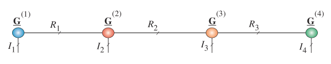
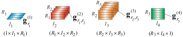
(b)

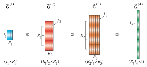
Figure 4.1: TT decomposition of a 4th-order tensor, $\underline{{\bf X}}$, for which the TT rank is $R_{1}=3,\;R_{2}=4,\;R_{3}=5$. (a) (Upper panel) Representation of the TT via a multilinear product of the cores, $\underline{{\bf X}}\cong\underline{{\bf G}}^{(1)}\,\times^{1}\,\underline{{\bf G}}^{(2)}\,\times^{1}\,\underline{{\bf G}}^{(3)}\times^{1}\,\underline{{\bf G}}^{(4)}=\mathopen{\hbox{\set@color${\langle}$}\kern-1.94444pt\leavevmode\hbox{\set@color${\langle}$}}\underline{{\bf G}}^{(1)},\underline{{\bf G}}^{(2)},\underline{{\bf G}}^{(3)},\underline{{\bf G}}^{(4)}\mathclose{\hbox{\set@color${\rangle}$}\kern-1.94444pt\leavevmode\hbox{\set@color${\rangle}$}}$, and (lower panel) an equivalent representation via the outer product of mode-2 fibers (sum of rank-1 tensors) in the form, $\underline{{\bf X}}\cong\sum_{r_{1}=1}^{R_{1}}\sum_{r_{2}=1}^{R_{2}}\sum_{r_{3}=1}^{R_{3}}\sum_{r_{4}=1}^{R_{4}}({\bf g}^{(1)}_{\,r_{1}}\;\circ\;{\bf g}^{(2)}_{\,r_{1},\,r_{2}}\;\circ\;{\bf g}^{(3)}_{\,r_{2},\,r_{3}}\;\circ\;{\bf g}^{(4)}_{\,r_{3}})$. (b) TT decomposition in a vectorized form represented via strong Kronecker products of block matrices, ${\bf x}\cong\widetilde{\bf G}^{(1)}\,|\!\!\otimes\!\!|\,\widetilde{\bf G}^{(2)}\,|\!\!\otimes\!\!|\,\widetilde{\bf G}^{(3)}\,|\!\!\otimes\!\!|\,\widetilde{\bf G}^{(4)}\in\mathbb{R}^{I_{1}I_{2}I_{3}I_{4}}$, where the block matrices are defined as $\widetilde{\bf G}^{(n)}\in\mathbb{R}^{R_{n-1}I_{n}\times R_{n}}$, with block vectors ${\bf g}^{(n)}_{r_{n-1},\,r_{n}}\in\mathbb{R}^{I_{n}\times 1}$, $n=1,\ldots,4$ and $R_{0}=R_{4}=1$.

Table 4.1: Equivalent representations of the Tensor Train decomposition (MPS with open boundary conditions) approximating an $N$th-order tensor $\underline{{\bf X}}\in\mathbb{R}^{I_{1}\times I_{2}\times\cdots\times I_{N}}$. It is assumed that the TT rank is ${\bf r}_{TT}=\{R_{1},R_{2},\ldots,R_{N-1}\}$, with $R_{0}=R_{N}=1$.

Tensor representation: Multilinear products of TT-cores $\underline{{\bf X}}=\underline{{\bf G}}^{(1)}\times^{1}\;\underline{{\bf G}}^{(2)}\times^{1}\;\cdots\;\times^{1}\;\underline{{\bf G}}^{(N)}\in\mathbb{R}^{I_{1}\times I_{2}\times\cdots\times I_{N}}$ with the 3rd-order cores $\underline{{\bf G}}^{(n)}\in\mathbb{R}^{R_{n-1}\times I_{n}\times R_{n}}$, $\;(n=1,2,\ldots,N)$ Tensor representation: Outer products $\underline{{\bf X}}=\displaystyle{\sum_{r_{1},\,r_{2},\ldots,r_{N-1}=1}^{R_{1},R_{2},\ldots,R_{N-1}}}\;\;{\bf g}^{(1)}_{\;1,r_{1}}\;\circ\;{\bf g}^{(2)}_{\;r_{1},\,r_{2}}\circ\cdots\circ\;{\bf g}^{(N-1)}_{\;r_{N-2},\,r_{N-1}}\;\circ\;{\bf g}^{(N)}_{\;r_{N-1},\,1}$ where ${\bf g}^{(n)}_{\;r_{n-1},\,r_{n}}=\underline{{\bf G}}^{(n)}(r_{n-1},:,r_{n})\in\mathbb{R}^{I_{n}}$ are fiber vectors. Vector representation: Strong Kronecker products ${\bf x}=\widetilde{\bf G}^{(1)}\;\,|\!\!\otimes\!\!|\,\;\widetilde{\bf G}^{(2)}\;\,|\!\!\otimes\!\!|\,\cdots\,|\!\!\otimes\!\!|\,\;\widetilde{\bf G}^{(N)}\in\mathbb{R}^{I_{1}I_{2}\cdots I_{N}}$,     where $\widetilde{\bf G}^{(n)}\in\mathbb{R}^{R_{n-1}I_{n}\times R_{n}}$ are block matrices with blocks ${\bf g}^{(n)}_{r_{n-1},r_{n}}\in\mathbb{R}^{I_{n}}$ Scalar representation $x_{\;i_{1},i_{2},\ldots,i_{N}}=\displaystyle{\sum_{r_{1},r_{2},\ldots,r_{N-1}=1}^{R_{1},R_{2},\ldots,R_{N-1}}}\!\!g^{(1)}_{\;1,\,i_{1},\,r_{1}}\;g^{(2)}_{\;r_{1},\,i_{2},\,r_{2}}\;\cdots\;g^{(N-1)}_{\;r_{N-2},\,i_{N-1},\,r_{N-1}}g^{(N)}_{\;r_{N-1},\,i_{N},1}$ where $g^{(n)}_{\;r_{n-1},\,i_{n},\,r_{n}}$ are entries of a 3rd-order core $\underline{{\bf G}}^{(n)}\in\mathbb{R}^{R_{n-1}\times I_{n}\times R_{n}}$ Slice (MPS) representation $x_{\;i_{1},\,i_{2},\ldots,i_{N}}={\bf G}^{(1)}_{i_{1}}\;{\bf G}^{(2)}_{i_{2}}\;\cdots\;{\bf G}^{(N)}_{i_{N}}$,     where ${\bf G}^{(n)}_{i_{n}}=\underline{{\bf G}}^{(n)}(:,i_{n},:)\in\mathbb{R}^{R_{n-1}\times R_{n}}$ are lateral slices of $\underline{{\bf G}}^{(n)}\in\mathbb{R}^{R_{n-1}\times I_{n}\times R_{n}}$

Table 4.2: Equivalent representations of the Tensor Chain (TC) decomposition (MPS with periodic boundary conditions) approximating an $N$th-order tensor $\underline{{\bf X}}\in\mathbb{R}^{I_{1}\times I_{2}\times\cdots\times I_{N}}$. It is assumed that the TC rank is ${\bf r}_{TC}=\{R_{1},R_{2},\ldots,R_{N-1},R_{N}\}$.

Tensor representation: Trace of multilinear products of cores $\underline{{\bf X}}=\mbox{Tr}\;(\underline{{\bf G}}^{(1)}\times^{1}\;\underline{{\bf G}}^{(2)}\times^{1}\;\cdots\;\times^{1}\;\underline{{\bf G}}^{(N)})\in\mathbb{R}^{I_{1}\times I_{2}\times\cdots\times I_{N}}$ with the 3rd-order cores $\underline{{\bf G}}^{(n)}\in\mathbb{R}^{R_{n-1}\times I_{n}\times R_{n}}$,  $R_{0}=R_{N}$,  $n=1,2,\ldots,N$ Tensor/Vector representation: Outer/Kronecker products $\underline{{\bf X}}=\displaystyle{\sum_{r_{1},\,r_{2},\ldots,r_{N}=1}^{R_{1},R_{2},\ldots,R_{N}}}\;\;{\bf g}^{(1)}_{\;r_{N},\,r_{1}}\;\circ\;{\bf g}^{(2)}_{\;r_{1},\,r_{2}}\;\circ\cdots\circ\;{\bf g}^{(N)}_{\;r_{N-1},\,r_{N}}\in\mathbb{R}^{I_{1}\times I_{2}\times\cdots\times I_{N}}$ ${\bf x}=\displaystyle{\sum_{r_{1},\,r_{2},\ldots,r_{N}=1}^{R_{1},R_{2},\ldots,R_{N}}}\;\;{\bf g}^{(1)}_{\;r_{N},\,r_{1}}\;\otimes_{L}\;{\bf g}^{(2)}_{\;r_{1},\,r_{2}}\;\otimes_{L}\cdots\otimes_{L}\;{\bf g}^{(N)}_{\;r_{N-1},\,r_{N}}\in\mathbb{R}^{I_{1}I_{2}\cdots I_{N}}$ where ${\bf g}^{(n)}_{\;r_{n-1},\;r_{n}}\in\mathbb{R}^{I_{n}}$ are fiber vectors within $\underline{{\bf G}}^{(n)}(r_{n-1},\,:,\,r_{n})\in\mathbb{R}^{I_{n}}$ Vector representation: Strong Kronecker products ${\bf x}=\displaystyle\sum_{r_{N}=1}^{R_{N}}(\widetilde{\bf G}^{(1)}_{\,r_{N}}\;\,|\!\!\otimes\!\!|\,\;\widetilde{\bf G}^{(2)}\;\,|\!\!\otimes\!\!|\,\cdots\,|\!\!\otimes\!\!|\,\;\widetilde{\bf G}^{(N-1)}\,|\!\!\otimes\!\!|\,\;\widetilde{\bf G}^{(N)}_{\,r_{N}})\in\mathbb{R}^{I_{1}\,I_{2}\cdots I_{N}}$     where $\widetilde{\bf G}^{(n)}\in\mathbb{R}^{R_{n-1}\,I_{n}\times R_{n}}$ are block matrices with blocks ${\bf g}^{(n)}_{\;r_{n-1},\,r_{n}}\in\mathbb{R}^{I_{n}}$, $\widetilde{\bf G}^{(1)}_{\,r_{N}}\in\mathbb{R}^{I_{1}\times R_{1}}$ is a matrix with blocks (columns) ${\bf g}^{(1)}_{\;r_{N},\,r_{1}}\in\mathbb{R}^{I_{1}}$, $\widetilde{\bf G}^{(N)}_{\,r_{N}}\in\mathbb{R}^{R_{N-1}\,I_{N}\times 1}$ is a block vector with blocks ${\bf g}^{(N)}_{\;r_{N-1},\,r_{N}}\in\mathbb{R}^{I_{N}}$ Scalar representations $x_{\;i_{1},\,i_{2},\ldots,i_{N}}=\mathop{\rm tr}\nolimits({\bf G}^{(1)}_{i_{1}}\,{\bf G}^{(2)}_{i_{2}}\cdots{\bf G}^{(N)}_{i_{N}})=\!\!\displaystyle\sum_{r_{N}=1}^{R_{N}}\!\!({\bf g}^{(1)\,\text{T}}_{r_{N},\,i_{1},\,:}\,{\bf G}^{(2)}_{i_{2}}\cdots{\bf G}^{(N-1)}_{i_{N-1}}{\bf g}^{(N)}_{:,\,i_{N},\,r_{N}})$ where ${\bf g}^{(1)}_{r_{N},\,i_{1},\,:}=\underline{{\bf G}}^{(1)}(r_{N},\,i_{1},\,:)\in\mathbb{R}^{R_{1}}$, ${\bf g}^{(N)}_{:,\,i_{N},\,r_{N}}\!=\underline{{\bf G}}^{(N)}(:,\,i_{N},\,r_{N})\in\mathbb{R}^{R_{N-1}}$

(a)

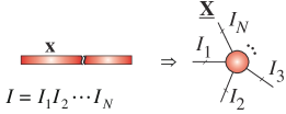
(b)

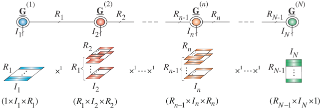
(c)

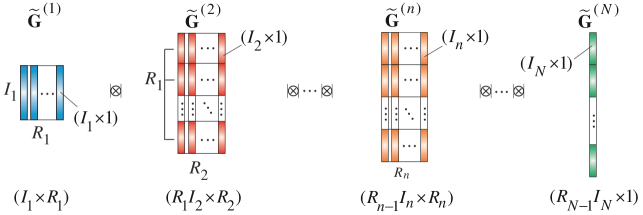
Figure 4.2: TT/MPS decomposition of an $N$th-order data tensor, $\underline{{\bf X}}$, for which the TT rank is $\{R_{1},R_{2},\ldots,R_{N-1}\}$. (a) Tensorization of a huge-scale vector, ${\bf x}\in\mathbb{R}^{I}$, into an $N$th-order tensor, $\underline{{\bf X}}\in\mathbb{R}^{I_{1}\times I_{2}\times\cdots\times I_{N}}$. (b) The data tensor can be represented exactly or approximately via a tensor train (TT/MPS), consisting of 3rd-order cores in the form $\underline{{\bf X}}\cong\underline{{\bf G}}^{(1)}\,\times^{1}\,\underline{{\bf G}}^{(2)}\,\times^{1}\,\cdots\times^{1}\,\underline{{\bf G}}^{(N)}=\mathopen{\hbox{\set@color${\langle}$}\kern-1.94444pt\leavevmode\hbox{\set@color${\langle}$}}\underline{{\bf G}}^{(1)},\underline{{\bf G}}^{(2)},\ldots,\underline{{\bf G}}^{(N)}\mathclose{\hbox{\set@color${\rangle}$}\kern-1.94444pt\leavevmode\hbox{\set@color${\rangle}$}}$, where $\underline{{\bf G}}^{(n)}\in\mathbb{R}^{R_{n-1}\times I_{n}\times R_{n}}$ for $n=1,2,\ldots,N$ with $R_{0}=R_{N}=1$. (c) Equivalently, using the strong Kronecker products, the TT tensor can be expressed in a vectorized form, ${\bf x}\cong\widetilde{\bf G}^{(1)}\,|\!\!\otimes\!\!|\,\widetilde{\bf G}^{(2)}\,|\!\!\otimes\!\!|\,\cdots\,|\!\!\otimes\!\!|\,\widetilde{\bf G}^{(N)}\in\mathbb{R}^{I_{1}I_{2}\cdots I_{N}}$, where the block matrices are defined as $\widetilde{\bf G}^{(n)}\in\mathbb{R}^{R_{n-1}I_{n}\times R_{n}}$, with blocks ${\bf g}^{(n)}_{r_{n-1},\,r_{n}}\in\mathbb{R}^{I_{n}\times 1}$.

The tensor train (TT/MPS) representation of an $N$th-order data tensor, $\underline{{\bf X}}\in\mathbb{R}^{I_{1}\times I_{2}\times\cdots\times I_{N}}$, can be described in several equivalent forms (see Figures 4.1, 4.2 and Table 4.1) listed below:

1. The entry-wise scalar form, given by

   $$x_{i_{1},i_{2},\ldots,i_{N}} \cong \sum_{r_{1},\,r_{2},\ldots,r_{N-1}=1}^{R_{1},R_{2},\ldots,R_{N-1}}g^{(1)}_{1,\,i_{1},\,r_{1}}\;g^{(2)}_{r_{1},\,i_{2},\,r_{2}}\cdots g^{(N)}_{r_{N-1},\,i_{N},1}.$$

2. The slice representation (see Figure 2.19) in the form

   $$x_{i_{1},i_{2},\ldots,i_{N}}\cong{\bf G}^{(1)}_{i_{1}}\;{\bf G}^{(2)}_{i_{2}}\cdots{\bf G}^{(N)}_{i_{N}},$$ (4.2)

   where the slice matrices are defined as

   $${\bf G}^{(n)}_{i_{n}}=\underline{{\bf G}}^{(n)}(:,i_{n},:)\in\mathbb{R}^{R_{n-1}\times R_{n}},\quad i_{n}=1,2,\ldots,I_{n}$$

   with ${\bf G}^{(n)}_{i_{n}}$ being the $i_{n}$th lateral slice of the core $\underline{{\bf G}}^{(n)}\in\mathbb{R}^{R_{n-1}\times I_{n}\times R_{n}}$, $n=1,2,\ldots,N$ and $R_{0}=R_{N}=1$.

3. The (global) tensor form, based on multilinear products (contraction) of cores (see Figure 4.1(a)) given by

   $$\underline{{\bf X}} \cong \underline{{\bf G}}^{(1)}\times^{1}\underline{{\bf G}}^{(2)}\times^{1}\cdots\times^{1}\underline{{\bf G}}^{(N-1)}\times^{1}\underline{{\bf G}}^{(N)}$$ (4.3)

   $$= \mathopen{\hbox{\set@color${\langle}$}\kern-1.94444pt\leavevmode\hbox{\set@color${\langle}$}}\underline{{\bf G}}^{(1)},\underline{{\bf G}}^{(2)},\ldots,\underline{{\bf G}}^{(N-1)},\underline{{\bf G}}^{(N)}\mathclose{\hbox{\set@color${\rangle}$}\kern-1.94444pt\leavevmode\hbox{\set@color${\rangle}$}},$$

   where the 3rd-order cores $\underline{{\bf G}}^{(n)}\in\mathbb{R}^{R_{n-1}\times I_{n}\times R_{n}}$, $n=1,2,\ldots,N$ and $R_{0}=R_{N}=1$ (see also Figure 4.2(b)).

4. The tensor form, expressed as a sum of rank-1 tensors (see Figure 4.1(a))

   $$\underline{{\bf X}}\cong\sum_{r_{1},\,r_{2},\ldots,r_{N-1}=1}^{R_{1},R_{2},\ldots,R_{N-1}}{\bf g}^{(1)}_{\,1,\,r_{1}}\;\circ\;{\bf g}^{(2)}_{\,r_{1},\,r_{2}}\;\circ\;\cdots\circ\;{\bf g}^{(N-1)}_{\,r_{N-2},\,r_{N-1}}\circ\;{\bf g}^{(N)}_{\,r_{N-1},\,1},$$ (4.4)

   where ${\bf g}^{(n)}_{r_{n-1},r_{n}}=\underline{{\bf G}}^{(n)}(r_{n-1},\,:,\,r_{n})\in\mathbb{R}^{I_{n}}$ are mode-2 fibers, $n=1,2,\ldots,N$ and $R_{0}=R_{N}=1$.

5. A vector form, expressed by Kronecker products of the fibers

   $${\bf x} \cong\sum_{r_{1},r_{2},\ldots,r_{N-1}=1}^{R_{1},R_{2},\ldots,R_{N-1}}{\bf g}^{(1)}_{\,1,\,r_{1}}\;\otimes_{L}\;{\bf g}^{(2)}_{\,r_{1},\,r_{2}}\;\otimes_{L}\;$$

   $$\quad\cdots\otimes_{L}\;{\bf g}^{(N-1)}_{\,r_{N-2},\,r_{N-1}}\otimes_{L}\;{\bf g}^{(N)}_{\,r_{N-1},\,1},$$ (4.5)

   where ${\bf x}=\mbox{vec}({\bf X})\in\mathbb{R}^{I_{1}I_{2}\cdots I_{N}}$.

6. An alternative vector form, produced by strong Kronecker products of block matrices (see Figure 4.1(b)) and Figure 4.2(c)), given by

   $${\bf x}\cong\widetilde{\bf G}^{(1)}\;\,|\!\!\otimes\!\!|\,\;\widetilde{\bf G}^{(2)}\;\,|\!\!\otimes\!\!|\,\cdots\,|\!\!\otimes\!\!|\,\widetilde{\bf G}^{(N)},\\$$ (4.6)

   where the block matrices $\widetilde{\bf G}^{(n)}\in\mathbb{R}^{R_{n-1}I_{n}\times R_{n}}$, for $n=1,2,\ldots,N$, consist of blocks ${\bf g}^{(n)}_{r_{n-1},r_{n}}\in\mathbb{R}^{I_{n}\times 1}$, $n=1,2,\ldots,N$, with $R_{0}=R_{N}=1$, and the symbol $\,|\!\!\otimes\!\!|\,$ denotes the strong Kronecker product.

Analogous relationships can be established for Tensor Chain (i.e., MPS with PBC (see Figure 2.19(b)) and summarized in Table 4.2.

4.2 Matrix TT Decomposition – Matrix Product Operator

The matrix tensor train, also called the Matrix Product Operator (MPO) with open boundary conditions (TT/MPO), is an important TN model which first represents huge-scale structured matrices, ${\bf X}\in\mathbb{R}^{I\times J}$, as $2N$th-order tensors, $\underline{{\bf X}}\in\mathbb{R}^{I_{1}\times J_{1}\times I_{2}\times J_{2}\times\cdots I_{N}\times J_{N}}$, where $I=I_{1}I_{2}\cdots I_{N}$ and $J=J_{1}J_{2}\cdots J_{N}$ (see Figures 4.3, 4.4 and Table 4.3). Then, the matrix TT/MPO converts such a $2N$th-order tensor into a chain (train) of 4th-order cores. It should be noted that the matrix TT decomposition is equivalent to the vector TT, created by merging all index pairs $(i_{n},j_{n})$ into a single index ranging from 1 to $I_{n}J_{n}$, in a reverse lexicographic order.

Similarly to the vector TT decomposition, a large scale $2N$th-order tensor, $\underline{{\bf X}}\in\mathbb{R}^{I_{1}\times J_{1}\times I_{2}\times J_{2}\times\cdots\times I_{N}\times J_{N}}$, can be represented in a TT/MPO format via the following mathematical representations:

1. The scalar (entry-wise) form

   $$x_{i_{1},j_{1},\ldots,i_{N},j_{N}} \cong \sum_{r_{1}=1}^{R_{1}}\sum_{r_{2}=1}^{R_{2}}\cdots\sum_{r_{N-1}=1}^{R_{N-1}}g^{(1)}_{\,1,\,i_{1},j_{1},r_{1}}\;g^{(2)}_{\,r_{1},\,i_{2},\,j_{2},\,r_{2}}$$ (4.7)

   $$\cdots g^{(N-1)}_{\,r_{N-2},\,i_{N-1},\,j_{N-1},\,r_{N-1}}\;g^{(N)}_{\,r_{N-1},\,i_{N},\,j_{N},\,1}.$$

2. The slice representation

   $$x_{i_{1},j_{1},\ldots,i_{N},j_{N}}\cong{\bf G}^{(1)}_{i_{1},j_{1}}\;{\bf G}^{(2)}_{i_{2},j_{2}}\cdots{\bf G}^{(N)}_{i_{N},j_{N}},\\$$ (4.8)

   where ${\bf G}^{(n)}_{i_{n},j_{n}}=\underline{{\bf G}}^{(n)}(:,\,i_{n},\,j_{n},\,:)\in\mathbb{R}^{R_{n-1}\times R_{n}}$ are slices of the cores $\underline{{\bf G}}^{(n)}\in\mathbb{R}^{R_{n-1}\times I_{n}\times J_{n}\times R_{n}}$, $\;\;n=1,2,\ldots,N$ and $R_{0}=R_{N}=1$.

3. The compact tensor form based on multilinear products (Figure 4.4(b))

   $$\underline{{\bf X}} \cong \underline{{\bf G}}^{(1)}\;\times^{1}\;\underline{{\bf G}}^{(2)}\;\times^{1}\;\cdots\times^{1}\;\underline{{\bf G}}^{(N)}$$ (4.9)

   $$= \mathopen{\hbox{\set@color${\langle}$}\kern-1.94444pt\leavevmode\hbox{\set@color${\langle}$}}\underline{{\bf G}}^{(1)},\underline{{\bf G}}^{(2)},\dots,\underline{{\bf G}}^{(N)}\mathclose{\hbox{\set@color${\rangle}$}\kern-1.94444pt\leavevmode\hbox{\set@color${\rangle}$}},$$

   where the TT-cores are defined as $\underline{{\bf G}}^{(n)}\in\mathbb{R}^{R_{n-1}\times I_{n}\times J_{n}\times R_{n}}$, $\;n=1,2,\ldots,N$ and $R_{0}=R_{N}=1$.

4. A matrix form, based on strong Kronecker products of block matrices (Figures 4.3(b) and 4.4(c))

   $${\bf X}\cong\widetilde{\bf G}^{(1)}\;\,|\!\!\otimes\!\!|\,\;\widetilde{\bf G}^{(2)}\;\,|\!\!\otimes\!\!|\,\cdots\,|\!\!\otimes\!\!|\,\;\widetilde{\bf G}^{(N)}\in\mathbb{R}^{I_{1}\cdots I_{N}\;\times\;J_{1}\cdots J_{N}},$$ (4.10)

   where $\widetilde{\bf G}^{(n)}\in\mathbb{R}^{R_{n-1}I_{n}\times R_{n}J_{n}}$ are block matrices with blocks ${\bf G}^{(n)}_{r_{n-1},r_{n}}\in\mathbb{R}^{I_{n}\times J_{n}}$ and the number of blocks is $R_{n-1}\times R_{n}$. In a special case, when the TT ranks $R_{n}=1,\;\forall n$, the strong Kronecker products simplify into standard (left) Kronecker products.

(a)

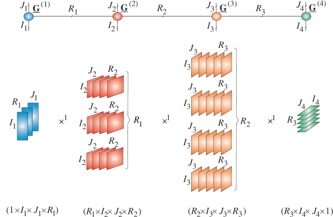
(b)

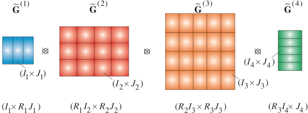
Figure 4.3: TT/MPO decomposition of a matrix, ${\bf X}\in\mathbb{R}^{I\times J}$, reshaped as an 8th-order tensor, $\underline{{\bf X}}\in\mathbb{R}^{I_{1}\times J_{1}\times\cdots\times I_{4}\times J_{4}}$, where $I=I_{1}I_{2}I_{3}I_{4}$ and $J=J_{1}J_{2}J_{3}J_{4}$. (a) Basic TT representation via multilinear products (tensor contractions) of cores $\underline{{\bf X}}=\underline{{\bf G}}^{(1)}\times^{1}\underline{{\bf G}}^{(2)}\times^{1}\underline{{\bf G}}^{(3)}\times^{1}\underline{{\bf G}}^{(4)}$, with $\underline{{\bf G}}^{(n)}\in\mathbb{R}^{R_{n-1}\times I_{n}\times R_{n}}$ for $R_{1}=3,R_{2}=4,R_{3}=5,R_{0}=R_{4}=1$. (b) Representation of a matrix or a matricized tensor via strong Kronecker products of block matrices, in the form ${\bf X}=\widetilde{\bf G}^{(1)}\,|\!\!\otimes\!\!|\,\widetilde{\bf G}^{(2)}\,|\!\!\otimes\!\!|\,\widetilde{\bf G}^{(3)}\,|\!\!\otimes\!\!|\,\widetilde{\bf G}^{(4)}\in\mathbb{R}^{I_{1}I_{2}I_{3}I_{4}\;\times\;J_{1}J_{2}J_{3}J_{4}}$.

(a)

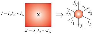
(b)

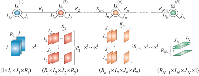
(c)

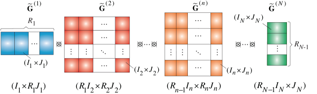
Figure 4.4: Representations of huge matrices by “linked” block matrices. (a) Tensorization of a huge-scale matrix, ${\bf X}\in\mathbb{R}^{I\times J}$, into a $2N$th-order tensor $\underline{{\bf X}}\in\mathbb{R}^{I_{1}\times J_{2}\times\cdots\times I_{N}\times J_{N}}$. (b) The TT/MPO decomposition of a huge matrix, ${\bf X}$, expressed by 4th-order cores, $\underline{{\bf G}}^{(n)}\in\mathbb{R}^{R_{n-1}\times I_{n}\times J_{n}\times R_{n}}$. (c) Alternative graphical representation of a matrix, ${\bf X}\in\mathbb{R}^{I_{1}I_{2}\cdots I_{N}\;\times\;J_{1}J_{2}\cdots J_{N}}$, via strong Kronecker products of block matrices $\widetilde{\bf G}^{(n)}\in\mathbb{R}^{R_{n-1}\,I_{n}\;\times\;R_{n}\,J_{n}}$ for $n=1,2,\ldots,N$ with $R_{0}=R_{N}=1$.

Table 4.3: Equivalent forms of the matrix Tensor Train decomposition (MPO with open boundary conditions) for a $2N$th-order tensor $\underline{{\bf X}}\in\mathbb{R}^{I_{1}\times J_{1}\times I_{2}\times J_{2}\times\cdots\times I_{N}\times J_{N}}$. It is assumed that the TT rank is $\{R_{1},R_{2},\ldots,R_{N-1}\}$, with $R_{0}=R_{N}=1$.

Tensor representation: Multilinear products (tensor contractions) $\underline{{\bf X}}=\underline{{\bf G}}^{(1)}\times^{1}\;\underline{{\bf G}}^{(2)}\times^{1}\cdots\times^{1}\;\underline{{\bf G}}^{(N-1)}\times^{1}\;\underline{{\bf G}}^{(N)}$             with 4th-order cores $\underline{{\bf G}}^{(n)}\in\mathbb{R}^{R_{n-1}\times I_{n}\times J_{n}\times R_{n}}$, $\quad(n=1,2,\ldots,N)$ Tensor representation: Outer products $\underline{{\bf X}}=\displaystyle{\sum_{r_{1},r_{2},\ldots,r_{N-1}=1}^{R_{1},R_{2},\ldots,R_{N-1}}}\;\;{\bf G}^{(1)}_{\;1,\,r_{1}}\;\circ\;{\bf G}^{(2)}_{\;r_{1},\,r_{2}}\circ\cdots\circ\;{\bf G}^{(N-1)}_{\;r_{N-2},\,r_{N-1}}\;\circ\;{\bf G}^{(N)}_{\;r_{N-1},\,1}$          where ${\bf G}^{(n)}_{\;r_{n-1},\,r_{n}}\in\mathbb{R}^{I_{n}\times J_{n}}$ are blocks of $\widetilde{\bf G}^{(n)}\in\mathbb{R}^{R_{n-1}I_{n}\times R_{n}J_{n}}$ Matrix representation: Strong Kronecker products ${\bf X}=\widetilde{\bf G}^{(1)}\;\,|\!\!\otimes\!\!|\,\;\widetilde{\bf G}^{(2)}\;\,|\!\!\otimes\!\!|\,\cdots\;\,|\!\!\otimes\!\!|\,\;\widetilde{\bf G}^{(N)}\in\mathbb{R}^{I_{1}\cdots I_{N}\;\times\;J_{1}\cdots J_{N}}$ where $\widetilde{\bf G}^{(n)}\in\mathbb{R}^{R_{n-1}I_{n}\times R_{n}J_{n}}$ are block matrices with blocks        $\underline{{\bf G}}^{(n)}(r_{n-1},:,:,r_{n})$ Scalar representation $x_{i_{1},j_{1},i_{2},j_{2},\ldots,i_{N},j_{N}}=\displaystyle{\sum_{r_{1},r_{2},\ldots,r_{N-1}=1}^{R_{1},R_{2},\ldots,R_{N-1}}}\;\;g^{(1)}_{\;1,i_{1},\,j_{1},\,r_{1}}\;g^{(2)}_{\;r_{1},\,i_{2},\,j_{2},\,r_{2}}\cdots\;g^{(N)}_{\;r_{N-1},\,i_{N},\,j_{N},1}$ where $g^{(n)}_{\;r_{n-1},\,i_{n},\,j_{n},\,r_{n}}$ are entries of a 4th-order core        $\underline{{\bf G}}^{(n)}\in\mathbb{R}^{R_{n-1}\times I_{n}\times J_{n}\times R_{n}}$ Slice (MPS) representation $x_{i_{1},j_{1},i_{2},j_{2},\ldots,i_{N},j_{N}}={\bf G}^{(1)}_{i_{1},j_{1}}\;{\bf G}^{(2)}_{i_{2},j_{2}}\cdots{\bf G}^{(N)}_{i_{N},j_{N}}$     where ${\bf G}^{(n)}_{i_{n},\,j_{n}}=\underline{{\bf G}}^{(n)}(:,i_{n},\,j_{n},:)\in\mathbb{R}^{R_{n-1}\times R_{n}}$ are slices of $\underline{{\bf G}}^{(n)}\in\mathbb{R}^{R_{n-1}\times I_{n}\times J_{n}\times R_{n}}$

The strong Kronecker product representation of a TT is probably the most comprehensive and useful form for displaying tensor trains in their vector/matrix form, since it allows us to perform many operations using relatively small block matrices.

Example. For two matrices (in the TT format) expressed via the strong Kronecker products, ${\bf A}=\tilde{\bf A}^{(1)}\,|\!\!\otimes\!\!|\,\tilde{\bf A}^{(2)}\,|\!\!\otimes\!\!|\,\cdots\,|\!\!\otimes\!\!|\,\tilde{\bf A}^{(N)}$ and $\;\;{\bf B}=\tilde{\bf B}^{(1)}\,|\!\!\otimes\!\!|\,\tilde{\bf B}^{(2)}\,|\!\!\otimes\!\!|\,\cdots\,|\!\!\otimes\!\!|\,\tilde{\bf B}^{(N)}$, their Kronecker product can be efficiently computed as ${\bf A}\otimes_{L}{\bf B}=\tilde{\bf A}^{(1)}\,|\!\!\otimes\!\!|\,\cdots\,|\!\!\otimes\!\!|\,\tilde{\bf A}^{(N)}\,|\!\!\otimes\!\!|\,\tilde{\bf B}^{(1)}\,|\!\!\otimes\!\!|\,\cdots\,|\!\!\otimes\!\!|\,\tilde{\bf B}^{(N)}$. Furthermore, if the matrices ${\bf A}$ and ${\bf B}$ have the same mode sizes, then their linear combination, ${\bf C}=\alpha{\bf A}+\beta{\bf B}$ can be compactly expressed as [158, 112, 113]

$${\bf C}=[\tilde{\bf A}^{(1)}\;\tilde{\bf B}^{(1)}]\,|\!\!\otimes\!\!|\,\left[\begin{array}[]{@{}c@{\hspace{1ex}}c@{}}\tilde{\bf A}^{(2)}\hfil\hskip 4.30554pt&{\bf 0}\\ {\bf 0}\hfil\hskip 4.30554pt&\tilde{\bf B}^{(2)}\end{array}\right]\,|\!\!\otimes\!\!|\,\cdots\,|\!\!\otimes\!\!|\,\left[\begin{array}[]{@{}c@{\hspace{1ex}}c@{}}\tilde{\bf A}^{(N-1)}\hfil\hskip 4.30554pt&0\\ 0\hfil\hskip 4.30554pt&\tilde{\bf B}^{(N-1)}\end{array}\right]\,|\!\!\otimes\!\!|\,\left[\begin{matrix}\alpha\tilde{\bf A}^{(N)}\\ \beta\tilde{\bf B}^{(N)}\end{matrix}\right].$$

Consider its reshaped tensor $\underline{{\bf C}}=\mathopen{\hbox{\set@color${\langle}$}\kern-1.94444pt\leavevmode\hbox{\set@color${\langle}$}}\underline{{\bf C}}^{(1)},\underline{{\bf C}}^{(2)},\ldots,\underline{{\bf C}}^{(N)}\mathclose{\hbox{\set@color${\rangle}$}\kern-1.94444pt\leavevmode\hbox{\set@color${\rangle}$}}$ in the TT format; then its cores $\underline{{\bf C}}^{(n)}\in\mathbb{R}^{R_{n-1}\times I_{n}\times J_{n}\times R_{n}}$, $n=1,2,\ldots,N$ can be expressed through their unfolding matrices, ${\bf C}^{(n)}_{<n>}\in\mathbb{R}^{R_{n-1}I_{n}\times R_{n}J_{n}}$, or equivalently by the lateral slices, ${\bf C}^{(n)}_{i_{n},j_{n}}\in\mathbb{R}^{R_{n-1}\times R_{n}}$, as follows

$${\bf C}_{i_{n},j_{n}}^{(n)} = \left[\begin{matrix}{\bf A}_{i_{n},j_{n}}^{(n)}&{\bf 0}\\ {\bf 0}&{\bf B}_{i_{n},j_{n}}^{(n)}\end{matrix}\right],\;\;n=2,3,\ldots,N-1,$$ (4.11)

while for the border cores

$${\bf C}_{i_{1},j_{1}}^{(1)}=\left[{\bf A}_{i_{1},j_{1}}^{(1)}\;{\bf B}_{i_{1},j_{1}}^{(1)}\right],\qquad{\bf C}_{i_{N},j_{N}}^{(N)} = \left[\begin{matrix}\alpha\;{\bf A}_{i_{N},j_{N}}^{(N)}\;\\ \;\beta\;{\bf B}_{i_{N},j_{N}}^{(N)}\end{matrix}\right]$$ (4.12)

for $i_{n}=1,2,\ldots,I_{n},\;j_{n}=1,2,\ldots,J_{N},\;n=1,2,\ldots,N$.

Note that the various mathematical and graphical representations of TT/MPS and TT/MPO can be used interchangeably for different purposes or applications. With these representations, all basic mathematical operations in TT format can be performed on the constitutive block matrices, even without the need to explicitly construct core tensors [158, 67].

Remark. In the TT/MPO paradigm, compression of large matrices is not performed by global (standard) low-rank matrix approximations, but by low-rank approximations of block-matrices (submatrices) arranged in a hierarchical (linked) fashion. However, to achieve a low-rank TT and consequently a good compression ratio, ranks of all the corresponding unfolding matrices of a specific structured data tensor must be low, i.e., their singular values must rapidly decrease to zero. While this is true for many structured matrices, unfortunately in general, this assumption does not hold.

4.3 Links Between CP, BTD Formats and TT/TC Formats

It is important to note that any specific TN format can be converted into the TT format. This very useful property is next illustrated for two simple but important cases which establish links between the CP and TT and the BTD and TT formats.

(a)

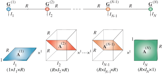
(b)

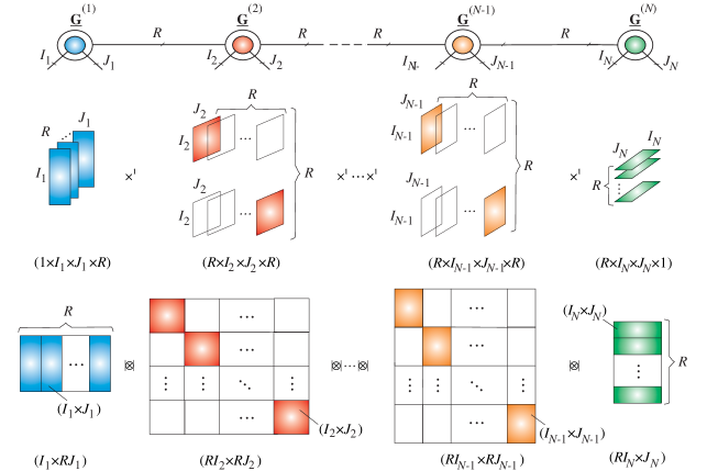
Figure 4.5: Links between the TT format and other tensor network formats. (a) Representation of the CP decomposition for an $N$th-order tensor, $\underline{{\bf X}}=\underline{{\bf I}}\times_{1}{\bf A}^{(1)}\times_{2}{\bf A}^{(2)}\cdots\times_{N}{\bf A}^{(N)}$, in the TT format. (b) Representation of the BTD model given by Eqs. (4.15) and (2) in the TT/MPO format. Observe that the TT-cores are very sparse and the TT ranks are $\{R,R,\ldots,R\}$. Similar relationships can be established straightforwardly for the TC format.

1. A tensor in the CP format, given by

   $$\underline{{\bf X}}=\sum_{r=1}^{R}{\bf a}_{r}^{(1)}\circ{\bf a}_{r}^{(2)}\circ\cdots\circ{\bf a}_{r}^{(N)},$$ (4.13)

   can be straightforwardly converted into the TT/MPS format as follows. Since each of the $R$ rank-1 tensors can be represented in the TT format of TT rank $(1,1,\ldots,1)$, using formulas (4.11) and (4.12), we have

   $$\underline{{\bf X}} = \sum_{r=1}^{R}\mathopen{\hbox{\set@color${\langle}$}\kern-1.94444pt\leavevmode\hbox{\set@color${\langle}$}}{\bf a}^{(1)\text{T}}_{r},{\bf a}^{(2)\text{T}}_{r},\ldots,{\bf a}^{(N)\text{T}}_{r}\mathclose{\hbox{\set@color${\rangle}$}\kern-1.94444pt\leavevmode\hbox{\set@color${\rangle}$}}$$

   $$= \mathopen{\hbox{\set@color${\langle}$}\kern-1.94444pt\leavevmode\hbox{\set@color${\langle}$}}\underline{{\bf G}}^{(1)},\underline{{\bf G}}^{(2)},\ldots,\underline{{\bf G}}^{(N-1)},\underline{{\bf G}}^{(N)}\mathclose{\hbox{\set@color${\rangle}$}\kern-1.94444pt\leavevmode\hbox{\set@color${\rangle}$}},$$

   where the TT-cores $\underline{{\bf G}}^{(n)}\in\mathbb{R}^{R\times I_{n}\times R}$ have diagonal lateral slices ${\bf G}^{(n)}(:,i_{n},:)={\bf G}^{(n)}_{i_{n}}=\mathop{\rm diag}\nolimits(a_{i_{n},1},a_{i_{n},2},\ldots,a_{i_{n},R})\in\mathbb{R}^{R\times R}$ for $n=2,3,\ldots,N-1$ and ${\bf G}^{(1)}={\bf A}^{(1)}\in\mathbb{R}^{I_{1}\times R}$ and ${\bf G}^{(N)}={\bf A}^{(N)\;\text{T}}\in\mathbb{R}^{R\times I_{N}}$ (see Figure 4.5(a)).

2. A more general Block Term Decomposition (BTD) for a $2N$th-order data tensor

   $$\underline{{\bf X}}=\sum_{r=1}^{R}({\bf A}_{r}^{(1)}\circ{\bf A}_{r}^{(2)}\circ\cdots\circ{\bf A}_{r}^{(N)})\in\mathbb{R}^{I_{1}\times J_{1}\times\cdots\times I_{N}\times J_{N}}$$ (4.15)

   with full rank matrices, ${\bf A}_{r}^{(n)}\in\mathbb{R}^{I_{n}\times J_{n}},\;\forall r$, can be converted into a matrix TT/MPO format, as illustrated in Figure 4.5(b).

   Note that (4.15) can be expressed in a matricized (unfolding) form via strong Kronecker products of block diagonal matrices (see formulas (4.11)), given by

   $${\bf X} = \sum_{r=1}^{R}({\bf A}_{r}^{(1)}\otimes_{L}{\bf A}_{r}^{(2)}\otimes_{L}\cdots\otimes_{L}{\bf A}_{r}^{(N)})$$

   $$= \widetilde{\bf G}^{(1)}\,|\!\!\otimes\!\!|\,\widetilde{\bf G}^{(2)}\,|\!\!\otimes\!\!|\,\cdots\,|\!\!\otimes\!\!|\,\widetilde{\bf G}^{(N)}\in\mathbb{R}^{I_{1}\cdots I_{N}\;\times\;J_{1}\cdots\times J_{N}},$$

   with the TT rank, $R_{n}=R$ for $n=1,2,\ldots N-1$, and the block diagonal matrices, $\widetilde{\bf G}^{(n)}=\mathop{\rm diag}\nolimits({\bf A}_{1}^{(n)},{\bf A}_{2}^{(n)},\ldots,{\bf A}_{R}^{(n)})\in\mathbb{R}^{RI_{n}\times RJ_{n}}$, for $n=2,3,\ldots,N-1$, while $\widetilde{\bf G}^{(1)}=[{\bf A}_{1}^{(1)},{\bf A}_{2}^{(1)},\ldots,{\bf A}_{R}^{(1)}]\in\mathbb{R}^{I_{1}\times RJ_{1}}$ is a row block matrix, and $\widetilde{\bf G}^{(N)}=\left[\begin{matrix}{\bf A}_{1}^{(N)}\\ \vdots\\ {\bf A}_{R}^{(N)}\end{matrix}\right]\in\mathbb{R}^{RI_{N}\times J_{N}}$ a column block matrix (see Figure 4.5(b)).

Several algorithms exist for decompositions in the form (4.15) and (2) [181, 14, 15]. In this way, TT/MPO decompositions for huge-scale structured matrices can be constructed indirectly.

4.4 Quantized Tensor Train (QTT) – Blessing of Dimensionality

The procedure of creating a higher-order tensor from lower-order original data is referred to as tensorization, while in a special case where each mode has a very small size 2, 3 or 4, it is referred to as quantization. In addition to vectors and matrices, lower-order tensors can also be reshaped into higher-order tensors. By virtue of quantization, low-rank TN approximations with high compression ratios can be obtained, which is not possible to achieve with original raw data formats. [157, 114].

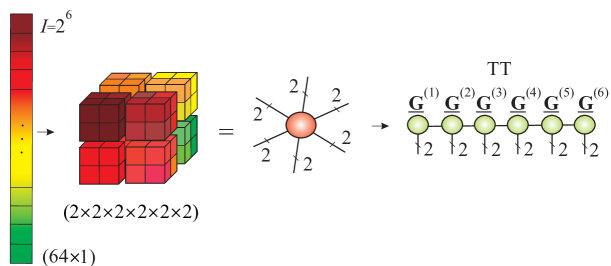
Figure 4.6: Concept of tensorization/quantization of a large-scale vector into a higher-order quantized tensor. In order to achieve a good compression ratio, we need to apply a suitable tensor decomposition such as the quantized TT (QTT) using 3rd-order cores, $\underline{{\bf X}}=\underline{{\bf G}}^{(1)}\times^{1}\underline{{\bf G}}^{(2)}\times^{1}\cdots\times^{1}\underline{{\bf G}}^{(6)}$.

Therefore, the quantization can be considered as a special form of tensorization where size of each mode is very small, typically 2 or 3. The concept of quantized tensor networks (QTN) was first proposed in [157] and [114], whereby low-size 3rd-order cores are sparsely interconnected via tensor contractions. The so obtained model often provides an efficient, highly compressed, and low-rank representation of a data tensor and helps to mitigate the curse of dimensionality, as illustrated below.

Example. The quantization of a huge vector, ${\bf x}\in\mathbb{R}^{I}$, $I=2^{K}$, can be achieved through reshaping to give a $(2\times 2\times\cdots\times 2)$ tensor $\underline{{\bf X}}$ of order $K$, as illustrated in Figure 4.6. For structured data such a quantized tensor, $\underline{{\bf X}}$, often admits low-rank TN approximation, so that a good compression of a huge vector ${\bf x}$ can be achieved by enforcing the maximum possible low-rank structure on the tensor network. Even more generally, an $N$th-order tensor, $\underline{{\bf X}}\in\mathbb{R}^{I_{1}\times\cdots\times I_{N}}$, with $I_{n}=q^{K_{n}}$, can be quantized in all modes simultaneously to yield a $(q\times q\times\cdots\times q)$ quantized tensor of higher-order and with small value of $q$.

Example. Since large-scale tensors (even of low-order) cannot be loaded directly into the computer memory, our approach to this problem is to represent the huge-scale data by tensor networks in a distributed and compressed TT format, so as to avoid the explicit requirement for unfeasible large computer memory.

In the example shown in Figure 4.7, the tensor train of a huge 3rd-order tensor is expressed by the strong Kronecker products of block tensors with relatively small 3rd-order tensor blocks. The QTT is mathematically represented in a distributed form via strong Kronecker products of block 5th-order tensors. Recall that the strong Kronecker product of two block core tensors, $\underline{\widetilde{\bf G}}^{(n)}\in\mathbb{R}^{R_{n-1}I_{n}\times R_{n}J_{n}\times K_{n}}$ and $\underline{\widetilde{\bf G}}^{(n+1)}\in\mathbb{R}^{R_{n}I_{n+1}\times R_{n+1}J_{n+1}\times K_{n+1}}$, is defined as the block tensor, $\underline{{\bf C}}=\underline{\widetilde{\bf G}}^{(n)}\,|\!\!\otimes\!\!|\,\underline{\widetilde{\bf G}}^{(n+1)}\in\mathbb{R}^{R_{n-1}I_{n}I_{n+1}\times R_{n+1}J_{n}J_{n+1}\times K_{n}K_{n+1}}$, with 3rd-order tensor blocks, $\underline{{\bf C}}_{r_{n-1},r_{n+1}}=\sum_{r_{n}=1}^{R_{n}}\underline{{\bf G}}^{(n)}_{r_{n-1},r_{n}}\otimes_{L}\underline{{\bf G}}^{(n+1)}_{r_{n},r_{n+1}}\in$
$\mathbb{R}^{I_{n}I_{n+1}\times J_{n}J_{n+1}\times K_{n}K_{n+1}}$, where $\underline{{\bf G}}^{(n)}_{r_{n-1},r_{n}}\in\mathbb{R}^{I_{n}\times J_{n}\times K_{n}}$ and $\underline{{\bf G}}^{(n+1)}_{r_{n},r_{n+1}}\in\mathbb{R}^{I_{n+1}\times J_{n+1}\times K_{n+1}}$ are the block tensors of $\underline{\widetilde{\bf G}}^{(n)}$ and $\underline{\widetilde{\bf G}}^{(n+1)}$, respectively.

In practice, a fine ($q=2,3,4$ ) quantization is desirable to create as many virtual (additional) modes as possible, thus allowing for the implementation of efficient low-rank tensor approximations. For example, the binary encoding ($q=2$) reshapes an $N$th-order tensor with $(2^{K_{1}}\times 2^{K_{2}}\times\cdots\times 2^{K_{N}})$ elements into a tensor of order $(K_{1}+K_{2}+\cdots+K_{N})$, with the same number of elements. In other words, the idea is to quantize each of the $n$ “physical” modes (dimensions) by replacing them with $K_{n}$ “virtual” modes, provided that the corresponding mode sizes, $I_{n}$, are factorized as $I_{n}=I_{n,1}I_{n,2}\cdots I_{n,K_{n}}$. This, in turn, corresponds to reshaping the $n$th mode of size $I_{n}$ into $K_{n}$ modes of sizes $I_{n,1},I_{n,2},\ldots,I_{n,K_{n}}$.

The TT decomposition applied to quantized tensors is referred to as the QTT, Quantics-TT or Quantized-TT, and was first introduced as a compression scheme for large-scale matrices [157], and also independently for more general settings.

(a)

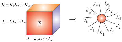
(b)

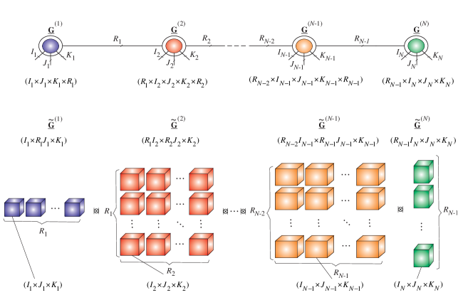
Figure 4.7: Tensorization/quantization of a huge-scale 3rd-order tensor into a higher order tensor and its TT representation. (a) Example of tensorization/quantization of a 3rd-order tensor, $\underline{{\bf X}}\in\mathbb{R}^{I\times J\times K}$, into a $3N$th-order tensor, assuming that the mode sizes can be factorized as, $I=I_{1}I_{2}\cdots I_{N}$, $J=J_{1}J_{2}\cdots J_{N}$ and $K=K_{1}K_{2}\cdots K_{N}$. (b) Decomposition of the high-order tensor via a generalized Tensor Train and its representation by the strong Kronecker product of block tensors as $\underline{{\bf X}}\cong\underline{\widetilde{\bf G}}^{(1)}\;\,|\!\!\otimes\!\!|\,\;\underline{\widetilde{\bf G}}^{(2)}\;\,|\!\!\otimes\!\!|\,\cdots\,|\!\!\otimes\!\!|\,\;\underline{\widetilde{\bf G}}^{(N)}\in\mathbb{R}^{I_{1}\cdots I_{N}\times J_{1}\cdots J_{N}\times K_{1}\cdots K_{N}}$, where each block $\underline{\widetilde{\bf G}}^{(n)}\in\mathbb{R}^{R_{n-1}I_{n}\times R_{n}J_{n}\times K_{n}}$ is also a 3rd-order tensor of size $(I_{n}\times J_{n}\times K_{n})$, for $n=1,2,\ldots,N$ with $R_{0}=R_{N}=1$. In the special case when $J=K=1$, the model simplifies into the standard TT/MPS model.

Table 4.4: Storage complexities of tensor decomposition models for an $N$th-order tensor, $\underline{{\bf X}}\in\mathbb{R}^{I_{1}\times I_{2}\times\cdots\times I_{N}}$, for which the original storage complexity is ${\cal{O}}(I^{N})$, where $I=\max\{I_{1},I_{2},\ldots,I_{N}\}$, while $R$ is the upper bound on the ranks of tensor decompositions considered, that is, $R=\max\{R_{1},R_{2},\ldots,R_{N-1}\}$ or $R=\max\{R_{1},R_{2},\ldots,R_{N}\}$.

1. Full (raw) tensor format ${\cal{O}}(I^{N})$ 2. CP ${\cal{O}}(NIR)$ 3. Tucker ${\cal{O}}(NIR+R^{N})$ 4. TT/MPS ${\cal{O}}(NIR^{2})$ 5. TT/MPO ${\cal{O}}(NI^{2}R^{2})$ 6. Quantized TT/MPS (QTT) ${\cal{O}}(NR^{2}\log_{q}(I))$ 7. QTT+Tucker ${\cal{O}}(NR^{2}\log_{q}(I)+NR^{3})$ 8. Hierarchical Tucker (HT) ${\cal{O}}(NIR+NR^{3})$

(a)

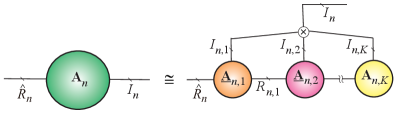
(b)

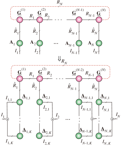
Figure 4.8: The QTT-Tucker or alternatively QTC-Tucker (Quantized Tensor-Chain-Tucker) format. (a) Distributed representation of a matrix ${\bf A}_{n}\in\mathbb{R}^{I_{n}\times\hat{R}_{n}}$ with a very large value of $I_{n}$ via QTT, by tensorization to a high-order quantized tensor, followed by QTT decomposition. (b) Distributed representation of a large-scale Tucker-$N$ model, $\underline{{\bf X}}\cong\underline{{\bf G}}\times_{1}{\bf A}_{1}\times{\bf A}_{2}\cdots\times_{N}{\bf A}_{N}$, via a quantized TC model in which the core tensor $\underline{{\bf G}}\in\mathbb{R}^{\hat{R}_{1}\times\hat{R}_{2}\times\cdots\times\hat{R}_{N}}$ and optionally all large-scale factor matrices ${\bf A}_{n}$ ($n=1,2,\ldots,N$) are represented by MPS models (for more detail see [68]).

The attractive properties of QTT are:

1. Not only QTT ranks are typically small (usually, below 20) but they are also almost independent of the data size (even for $I=2^{50}$), thus providing a logarithmic (sub-linear) reduction of storage requirements from ${\cal{O}}(I^{N})$ to ${\cal{O}}(NR^{2}\log_{q}(I))$ which is referred to as super-compression [114, 111, 112, 68, 70]. Comparisons of the storage complexity of various tensor formats are given in Table 4.4.

2. Compared to the TT decomposition (without quantization), the QTT format often represents deep structures in the data by introducing “virtual” dimensions or modes. For data which exhibit high degrees of structure, the high compressibility of the QTT approximation is a consequence of the better separability properties of the quantized tensor.

3. The fact that the QTT ranks are often moderate or even low offers unique advantages in the context of big data analytics (see [114, 115, 112] and references therein), together with high efficiency of multilinear algebra within the TT/QTT algorithms which rests upon the well-posedness of the low-rank TT approximations.

The ranks of the QTT format often grow dramatically with data size, but with a linear increase in the approximation accuracy. To overcome this problem, Dolgov and Khoromskij proposed the QTT-Tucker format [68] (see Figure 4.8), which exploits the TT approximation not only for the Tucker core tensor, but also for the factor matrices. This model naturally admits distributed computation, and often yields bounded ranks, thus avoiding the curse of dimensionality.

The TT/QTT tensor networks have already found application in very large-scale problems in scientific computing, such as in eigenanalysis, super-fast Fourier transforms, and in solving huge systems of large linear equations (see [68, 102, 70, 218, 120, 123] and references therein).

4.5 Basic Operations in TT Formats

For big tensors in their TT formats, basic mathematical operations, such as the addition, inner product, computation of tensor norms, Hadamard and Kronecker product, and matrix-by-vector and matrix-by-matrix multiplications can be very efficiently performed using block (slice) matrices of individual (relatively small size) core tensors.

Consider two $N$th-order tensors in the TT format

$$\underline{{\bf X}} = \mathopen{\hbox{\set@color${\langle}$}\kern-1.94444pt\leavevmode\hbox{\set@color${\langle}$}}\underline{{\bf X}}^{(1)},\underline{{\bf X}}^{(2)},\ldots,\underline{{\bf X}}^{(N)}\mathclose{\hbox{\set@color${\rangle}$}\kern-1.94444pt\leavevmode\hbox{\set@color${\rangle}$}}\in\mathbb{R}^{I_{1}\times I_{2}\times\cdots\times I_{N}}$$

$$\underline{{\bf Y}} = \mathopen{\hbox{\set@color${\langle}$}\kern-1.94444pt\leavevmode\hbox{\set@color${\langle}$}}\underline{{\bf Y}}^{(1)},\underline{{\bf Y}}^{(2)},\ldots,\underline{{\bf Y}}^{(N)}\mathclose{\hbox{\set@color${\rangle}$}\kern-1.94444pt\leavevmode\hbox{\set@color${\rangle}$}}\in\mathbb{R}^{I_{1}\times I_{2}\times\cdots\times I_{N}},$$

for which the TT ranks are ${\bf r}_{X}=\{R_{1},R_{2},\ldots,R_{N-1}\}$ and ${\bf r}_{Y}=\{\tilde{R}_{1},\tilde{R}_{2},\ldots,\tilde{R}_{N-1}\}$. The following operations can then be performed directly in the TT formats.

Tensor addition. The sum of two tensors

$$\underline{{\bf Z}}=\underline{{\bf X}}+\underline{{\bf Y}}=\mathopen{\hbox{\set@color${\langle}$}\kern-1.94444pt\leavevmode\hbox{\set@color${\langle}$}}\underline{{\bf Z}}^{(1)},\underline{{\bf Z}}^{(2)},\ldots,\underline{{\bf Z}}^{(N)}\mathclose{\hbox{\set@color${\rangle}$}\kern-1.94444pt\leavevmode\hbox{\set@color${\rangle}$}}\in\mathbb{R}^{I_{1}\times I_{2}\times\cdots\times I_{N}}$$ (4.17)

has the TT rank ${\bf r}_{Z}={\bf r}_{X}+{\bf r}_{Y}$ and can be expressed via lateral slices of the cores $\underline{{\bf Z}}\in\mathbb{R}^{R_{n-1}\times I_{n}\times R_{n}}$ as

$${\bf Z}_{i_{n}}^{(n)} = \left[\begin{matrix}{\bf X}_{i_{n}}^{(n)}&{\bf 0}\\ {\bf 0}&{\bf Y}_{i_{n}}^{(n)}\end{matrix}\right],\;\;n=2,3,\ldots,N-1.$$ (4.18)

For the border cores, we have

$${\bf Z}_{i_{1}}^{(1)}=\left[{\bf X}_{i_{1}}^{(1)}\;{\bf Y}_{i_{1}}^{(1)}\right],\qquad{\bf Z}_{i_{N}}^{(N)} = \left[\begin{matrix}{\bf X}_{i_{N}}^{(N)}\;\\ \;{\bf Y}_{i_{N}}^{(N)}\end{matrix}\right]$$ (4.19)

for $i_{n}=1,2,\ldots,I_{n},\;\ n=1,2,\ldots,N$.

Hadamard product. The computation of the Hadamard (element-wise) product, $\underline{{\bf Z}}=\underline{{\bf X}}\circledast\underline{{\bf Y}}$, of two tensors, ${\bf X}$ and ${\bf Y}$, of the same order and the same size can be performed very efficiently in the TT format by expressing the slices of the cores, $\underline{{\bf Z}}\in\mathbb{R}^{R_{n-1}\times I_{n}\times R_{n}}$, as

$${\bf Z}_{i_{n}}^{(n)}={\bf X}_{i_{n}}^{(n)}\otimes{\bf Y}_{i_{n}}^{(n)},\quad n=1,\ldots,N,\;\;i_{n}=1,\ldots,I_{n}.$$ (4.20)

This increases the TT ranks for the tensor $\underline{{\bf Z}}$ to at most $R_{n}\tilde{R}_{n}$, $n=1,2,\ldots,N$, but the associated computational complexity can be reduced from being exponential in $N$, ${\cal{O}}(I^{N})$, to being linear in both $I$ and $N$, ${\cal{O}}(IN(R\tilde{R})^{2}))$.

Super fast Fourier transform of a tensor in the TT format (MATLAB functions: fftn$(\underline{{\bf X}})$ and fft$(\underline{{\bf X}}^{(n)},[],2)$) can be computed as

$${\cal{F}}(\underline{{\bf X}}) = \mathopen{\hbox{\set@color${\langle}$}\kern-1.94444pt\leavevmode\hbox{\set@color${\langle}$}}{\cal{F}}(\underline{{\bf X}}^{(1)}),{\cal{F}}(\underline{{\bf X}}^{(2)}),\ldots,{\cal{F}}(\underline{{\bf X}}^{(N)})\mathclose{\hbox{\set@color${\rangle}$}\kern-1.94444pt\leavevmode\hbox{\set@color${\rangle}$}}$$ (4.21)

$$= {\cal{F}}(\underline{{\bf X}}^{(1)})\times^{1}{\cal{F}}(\underline{{\bf X}}^{(2)})\times^{1}\cdots\times^{1}{\cal{F}}(\underline{{\bf X}}^{(N)}).$$

It should be emphasized that performing computation of the FFT on relatively small core tensors $\underline{{\bf X}}^{(n)}\in\mathbb{R}^{R_{n-1}\times I_{n}\times R_{n}}$ reduces dramatically computational complexity under condition that a data tensor admits low-rank TT approximation. This approach is referred to as the super fast Fourier transform (SFFT) in TT format. Wavelets, DCT, and other linear integral transformations admit a similar form to the SFFT in (4.21), for example, for the wavelet transform in the TT format, we have

$${\cal{W}}(\underline{{\bf X}}) = \mathopen{\hbox{\set@color${\langle}$}\kern-1.94444pt\leavevmode\hbox{\set@color${\langle}$}}{\cal{W}}(\underline{{\bf X}}^{(1)}),{\cal{W}}(\underline{{\bf X}}^{(2)}),\ldots,{\cal{W}}(\underline{{\bf X}}^{(N)})\mathclose{\hbox{\set@color${\rangle}$}\kern-1.94444pt\leavevmode\hbox{\set@color${\rangle}$}}$$ (4.22)

$$= {\cal{W}}(\underline{{\bf X}}^{(1)})\times^{1}{\cal{W}}(\underline{{\bf X}}^{(2)})\times^{1}\cdots\times^{1}{\cal{W}}(\underline{{\bf X}}^{(N)}).$$

The N-D discrete convolution in a TT format of tensors $\underline{{\bf X}}\in\mathbb{R}^{I_{1}\times\cdots\times I_{N}}$ with TT rank $\{R_{1},R_{2},\ldots,R_{N-1}\}$ and $\underline{{\bf Y}}\in\mathbb{R}^{J_{1}\times\cdots\times J_{N}}$ with TT rank $\{Q_{1},Q_{2},\ldots,Q_{N-1}\}$ can be computed as

$$\underline{{\bf Z}} = \underline{{\bf X}}\ast\underline{{\bf Y}}$$

$$= \mathopen{\hbox{\set@color${\langle}$}\kern-1.94444pt\leavevmode\hbox{\set@color${\langle}$}}\underline{{\bf Z}}^{(1)},\underline{{\bf Z}}^{(2)},\ldots,\underline{{\bf Z}}^{(N)}\mathclose{\hbox{\set@color${\rangle}$}\kern-1.94444pt\leavevmode\hbox{\set@color${\rangle}$}}\in\mathbb{R}^{(I_{1}+J_{1}-1)\times(I_{2}+J_{2}-1)\times\cdots\times(I_{N}+J_{N}-1)},$$

with the TT-cores given by

$$\underline{{\bf Z}}^{(n)}=\underline{{\bf X}}^{(n)}\boxdot_{2}\underline{{\bf Y}}^{(n)}\in\mathbb{R}^{(R_{n-1}Q_{n-1})\times(I_{n}+J_{n}-1)\times(R_{n}Q_{n})},$$ (4.24)

or, equivalently, using the standard convolution $\underline{{\bf Z}}^{(n)}(s_{n-1},:,s_{n})=\underline{{\bf X}}^{(n)}(r_{n-1},:,r_{n})\ast\underline{{\bf Y}}^{(n)}(q_{n-1},:,q_{n})\in\mathbb{R}^{(I_{n}+J_{n}-1)}$ for $s_{n}=1,2,\ldots,R_{n}Q_{n}$ and $n=1,2,\ldots,N$, $\;R_{0}=R_{N}=1$.

Inner product. The computation of the inner (scalar, dot) product of two $N$th-order tensors, $\underline{{\bf X}}=\mathopen{\hbox{\set@color${\langle}$}\kern-1.94444pt\leavevmode\hbox{\set@color${\langle}$}}\underline{{\bf X}}^{(1)},\underline{{\bf X}}^{(2)},\ldots,\underline{{\bf X}}^{(N)}\mathclose{\hbox{\set@color${\rangle}$}\kern-1.94444pt\leavevmode\hbox{\set@color${\rangle}$}}\in\mathbb{R}^{I_{1}\times I_{2}\times\cdots\times I_{N}}$ and ${\bf Y}=\mathopen{\hbox{\set@color${\langle}$}\kern-1.94444pt\leavevmode\hbox{\set@color${\langle}$}}\underline{{\bf Y}}^{(1)},\underline{{\bf Y}}^{(2)},\ldots,\underline{{\bf Y}}^{(N)}\mathclose{\hbox{\set@color${\rangle}$}\kern-1.94444pt\leavevmode\hbox{\set@color${\rangle}$}}\in\mathbb{R}^{I_{1}\times I_{2}\times\cdots\times I_{N}}$, is given by

$$\langle\underline{{\bf X}},\underline{{\bf Y}}\rangle = \langle\mbox{vec}(\underline{{\bf X}}),\mbox{vec}(\underline{{\bf Y}})\rangle$$

$$= \sum_{i_{1}=1}^{I_{1}}\cdots\sum_{i_{N}=1}^{I_{N}}x_{i_{1}\dots i_{n}}\;y_{i_{1}\cdots i_{N}}$$

and has the complexity of ${\cal{O}}(I^{N})$ in the raw tensor format. In TT formats, the inner product can be computed with the reduced complexity of only ${\cal{O}}(NI(R^{2}\tilde{R}+R\tilde{R}^{2}))$ when the inner product is calculated by moving TT-cores from left to right and performing calculations on relatively small matrices, ${\bf S}_{n}=\underline{{\bf X}}^{(n)}\times^{1,2}_{1,2}(\underline{{\bf Y}}^{(n)}\times_{1}{\bf S}_{n-1})\in\mathbb{R}^{R_{n}\times\widetilde{R}_{n}}$ for $n=1,2,\ldots,N$. The results are then sequentially multiplied by the next core $\underline{{\bf Y}}^{(n+1)}$ (see Algorithm 9).

Computation of the Frobenius norm. In a similar way, we can efficiently compute the Frobenius norm of a tensor, $\|\underline{{\bf X}}\|_{F}=\sqrt{\langle\underline{{\bf X}},\underline{{\bf X}}\rangle}$, in the TT format. For the so-called $n$-orthogonal TT format, it is easy to show that

$$\|\underline{{\bf X}}\|_{F}=\|\underline{{\bf X}}^{(n)}\|_{F}.$$ (4.26)

0:  $N$th-order tensors, $\underline{{\bf X}}=\mathopen{\hbox{\set@color${\langle}$}\kern-1.94444pt\leavevmode\hbox{\set@color${\langle}$}}\underline{{\bf X}}^{(1)},\underline{{\bf X}}^{(2)},\ldots,\underline{{\bf X}}^{(N)}\mathclose{\hbox{\set@color${\rangle}$}\kern-1.94444pt\leavevmode\hbox{\set@color${\rangle}$}}\in\mathbb{R}^{I_{1}\times I_{2}\times\cdots\times I_{N}}$ and ${\bf Y}=\mathopen{\hbox{\set@color${\langle}$}\kern-1.94444pt\leavevmode\hbox{\set@color${\langle}$}}\underline{{\bf Y}}^{(1)},\underline{{\bf Y}}^{(2)},\ldots,\underline{{\bf Y}}^{(N)}\mathclose{\hbox{\set@color${\rangle}$}\kern-1.94444pt\leavevmode\hbox{\set@color${\rangle}$}}\in\mathbb{R}^{I_{1}\times I_{2}\times\cdots\times I_{N}}$ in TT formats, with TT-cores $\underline{{\bf X}}\in\mathbb{R}^{R_{n-1}\times I_{n}\times R_{n}}$ and $\underline{{\bf Y}}\in\mathbb{R}^{\widetilde{R}_{n-1}\times I_{n}\times\widetilde{R}_{n}}$ and $R_{0}=\widetilde{R}_{0}=R_{N}=\widetilde{R}_{N}=1$ 0:  Inner product $\langle\underline{{\bf X}},\underline{{\bf Y}}\rangle=\mbox{vec}(\underline{{\bf X}})^{\text{T}}\mbox{vec}(\underline{{\bf Y}})$ 1:  Initialization ${\bf S}_{0}=1$ 2:  for $n=1$ to $N$ do 3:     ${\bf Z}^{(n)}_{(1)}={\bf S}_{n-1}{\bf Y}^{(n)}_{(1)}\in\mathbb{R}^{R_{n-1}\times I_{n}\widetilde{R}_{n}}$ 4:     ${\bf S}_{n}={\bf X}^{(n)\;\text{T}}_{<2>}{\bf Z}^{(n)}_{<2>}\in\mathbb{R}^{R_{n}\times\widetilde{R}_{n}}$ 5:  end for 6:  return  Scalar $\langle\underline{{\bf X}},\underline{{\bf Y}}\rangle={\bf S}_{N}\in\mathbb{R}^{R_{N}\times\widetilde{R}_{N}}=\mathbb{R}$, with $R_{N}=\widetilde{R}_{N}=1$

Algorithm 9 Inner product of two large-scale tensors in the TT Format [158, 67]

Matrix-by-vector multiplication. Consider a huge-scale matrix equation (see Figure 4.9 and Figure 4.10)

$${\bf A}{\bf x}={\bf y},$$ (4.27)

where ${\bf A}\in\mathbb{R}^{I\times J}$, $\;\;{\bf x}\in\mathbb{R}^{J}$ and ${\bf y}\in\mathbb{R}^{I}$ are represented approximately in the TT format, with $I=I_{1}I_{2}\cdots I_{N}$ and $J=J_{1}J_{2}\cdots J_{N}$. As shown in Figure 4.9(a), the cores are defined as $\underline{{\bf A}}^{(n)}\in\mathbb{R}^{P_{n-1}\times I_{n}\times J_{n}\times P_{n}}$, $\;\underline{{\bf X}}^{(n)}\in\mathbb{R}^{R_{n-1}\times J_{n}\times R_{n}}$ and $\;\underline{{\bf Y}}^{(n)}\in\mathbb{R}^{Q_{n-1}\times I_{n}\times Q_{n}}$.

Upon representing the entries of the matrix ${\bf A}$ and vectors ${\bf x}$ and ${\bf y}$ in their tensorized forms, given by

$$\underline{{\bf A}} = \displaystyle{\sum_{p_{1},p_{2},\ldots,p_{N-1}=1}^{P_{1},P_{2},\ldots,P_{N-1}}}\;\;{\bf A}^{(1)}_{\;1,p_{1}}\;\circ\;{\bf A}^{(2)}_{\;p_{1},p_{2}}\circ\cdots\circ\;{\bf A}^{(N)}_{\;p_{N-1},1}$$

$$\underline{{\bf X}} = \displaystyle{\sum_{r_{1},r_{2},\ldots,r_{N-1}=1}^{R_{1},R_{2},\ldots,R_{N-1}}}\;\;{\bf x}^{(1)}_{\;r_{1}}\;\circ\;{\bf x}^{(2)}_{\;r_{1},r_{2}}\circ\cdots\circ\;{\bf x}^{(N)}_{\;r_{N-1}}$$ (4.28)

$$\underline{{\bf Y}} = \displaystyle{\sum_{q_{1},q_{2},\ldots,q_{N-1}=1}^{Q_{1},Q_{2},\ldots,Q_{N-1}}}\;\;{\bf y}^{(1)}_{\;q_{1}}\;\circ\;{\bf y}^{(2)}_{\;q_{1},q_{2}}\circ\cdots\circ\;{\bf y}^{(N)}_{\;q_{N-1}},$$

we arrive at a simple formula for the tubes of the tensor $\underline{{\bf Y}}$, in the form

$${\bf y}^{(n)}_{q_{n-1},q_{n}}={\bf y}^{(n)}_{\overline{r_{n-1}\,p_{n-1}},\;\overline{r_{n}\,p_{n}}}={\bf A}^{(n)}_{p_{n-1},\,p_{n}}\;{\bf x}^{(n)}_{r_{n-1},\,r_{n}}\in\mathbb{R}^{I_{n}},$$

with $Q_{n}=P_{n}\,R_{n}$ for $n=1,2,\ldots,N$.

(a)

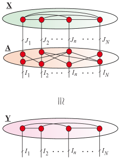
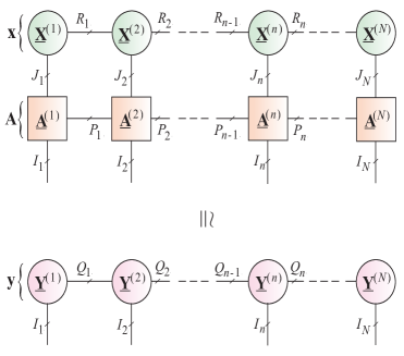
(b)

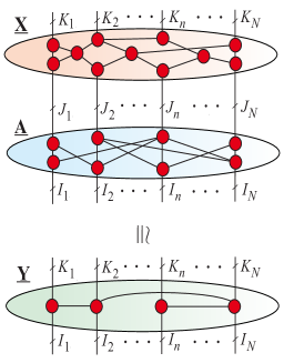
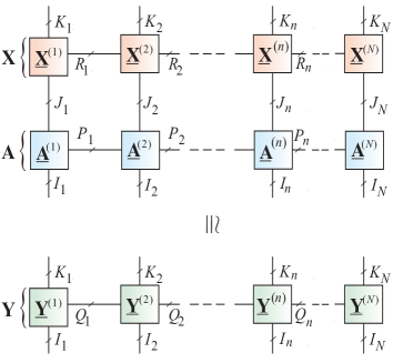
Figure 4.9: Linear systems represented by arbitrary tensor networks (left) and TT networks (right) for (a) ${\bf A}{\bf x}\cong{\bf y}$ and (b) ${\bf A}{\bf X}\cong{\bf Y}$.

(a)

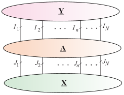
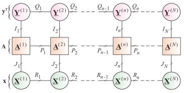
(b)

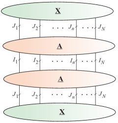
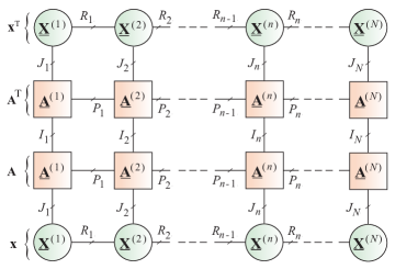
Figure 4.10: Representation of typical cost functions by arbitrary TNs and by TT networks: (a) $J_{1}({\bf x})={\bf y}^{\text{T}}{\bf A}{\bf x}$ and (b) $J_{2}({\bf x})={\bf x}^{\text{T}}{\bf A}^{\text{T}}{\bf A}{\bf x}$. Note that tensors $\underline{{\bf A}}$, $\underline{{\bf X}}$ and $\underline{{\bf Y}}$ can be, in general, approximated by any TNs that provide good low-rank representations.

Furthermore, by representing the matrix ${\bf A}$ and vectors ${\bf x}$, ${\bf y}$ via the strong Kronecker products

$${\bf A} = \tilde{\bf A}^{(1)}\,|\!\!\otimes\!\!|\,\tilde{\bf A}^{(2)}\,|\!\!\otimes\!\!|\,\cdots\,|\!\!\otimes\!\!|\,\tilde{\bf A}^{(N)}$$

$${\bf x} = \tilde{\bf X}^{(1)}\,|\!\!\otimes\!\!|\,\tilde{\bf X}^{(2)}\,|\!\!\otimes\!\!|\,\cdots\,|\!\!\otimes\!\!|\,\tilde{\bf X}^{(N)}$$ (4.29)

$${\bf y} = \tilde{\bf Y}^{(1)}\,|\!\!\otimes\!\!|\,\tilde{\bf Y}^{(2)}\,|\!\!\otimes\!\!|\,\cdots\,|\!\!\otimes\!\!|\,\tilde{\bf Y}^{(N)},$$

with $\tilde{\bf A}^{(n)}\in\mathbb{R}^{P_{n-1}I_{n}\times J_{n}P_{n}},\;\;\tilde{\bf X}^{(n)}\in\mathbb{R}^{R_{n-1}J_{n}\times R_{n}}$ and $\tilde{\bf Y}^{(n)}\in\mathbb{R}^{Q_{n-1}I_{n}\times Q_{n}}$, we can establish a simple relationship

$$\tilde{\bf Y}^{(n)}=\tilde{\bf A}^{(n)}\;\,|\!\bullet\!|\,\;\tilde{\bf X}^{(n)}\in\mathbb{R}^{R_{n-1}\,P_{n-1}\,I_{n}\times R_{n}\,P_{n}},\quad n=1,\ldots,N,$$ (4.30)

where the operator $\,|\!\bullet\!|\,$ represents the C (Core) product of two block matrices.

The C product of a block matrix ${\bf A}^{(n)}\in\mathbb{R}^{P_{n-1}I_{n}\times P_{n}J_{n}}$ with blocks ${\bf A}^{(n)}_{p_{n-1},p_{n}}\in\mathbb{R}^{I_{n}\times J_{n}}$, and a block matrix ${\bf B}^{(n)}\in\mathbb{R}^{R_{n-1}J_{n}\times R_{n}K_{n}}$, with blocks ${\bf B}^{(n)}_{r_{n-1},r_{n}}\in\mathbb{R}^{J_{n}\times K_{n}}$, is defined as ${\bf C}^{(n)}={\bf A}^{(n)}\;\,|\!\bullet\!|\,\;{\bf B}^{(n)}\in\mathbb{R}^{Q_{n-1}I_{n}\times Q_{n}K_{n}}$, the blocks of which are given by ${\bf C}^{(n)}_{q_{n-1},q_{n}}={\bf A}^{(n)}_{p_{n-1},p_{n}}{\bf B}^{(n)}_{r_{n-1},r_{n}}\in\mathbb{R}^{I_{n}\times K_{n}}$, where $\;q_{n}=\overline{p_{n}r_{n}}$, as illustrated in Figure 4.11.

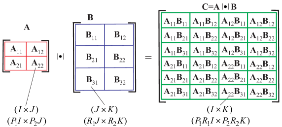
Figure 4.11: Graphical illustration of the C product of two block matrices.

Table 4.5: Basic operations on tensors in TT formats, where $\underline{{\bf X}}=\underline{{\bf X}}^{(1)}\times^{1}\underline{{\bf X}}^{(2)}\times^{1}\cdots\times^{1}\underline{{\bf X}}^{(N)}\in\mathbb{R}^{I_{1}\times I_{2}\times\cdots\times I_{N}}$, $\underline{{\bf Y}}=\underline{{\bf Y}}^{(1)}\times^{1}\underline{{\bf Y}}^{(2)}\times^{1}\cdots\times^{1}\underline{{\bf Y}}^{(N)}\in\mathbb{R}^{J_{1}\times J_{2}\times\cdots\times J_{N}}$, and $\underline{{\bf Z}}=\underline{{\bf Z}}^{(1)}\times^{1}\underline{{\bf Z}}^{(2)}\times^{1}\cdots\times^{1}\underline{{\bf Z}}^{(N)}\in\mathbb{R}^{K_{1}\times K_{2}\times\cdots\times K_{N}}$.

Operation                        TT-cores $\underline{{\bf Z}}=\underline{{\bf X}}+\underline{{\bf Y}}=\left(\underline{{\bf X}}^{(1)}\oplus_{2}\underline{{\bf Y}}^{(1)}\right)\times^{1}\left(\underline{{\bf X}}^{(2)}\oplus_{2}\underline{{\bf Y}}^{(2)}\right)\times^{1}\cdots\times^{1}\left(\underline{{\bf X}}^{(N)}\oplus_{2}\underline{{\bf Y}}^{(N)}\right)$ $\underline{{\bf Z}}^{(n)}=\underline{{\bf X}}^{(n)}\oplus_{2}\underline{{\bf Y}}^{(n)}$, with TT core slices ${\bf Z}^{(n)}_{i_{n}}={\bf X}^{(n)}_{i_{n}}\oplus{\bf Y}^{(n)}_{i_{n}},\;(I_{n}=J_{n}=K_{n},\;\forall n)$ $\underline{{\bf Z}}=\underline{{\bf X}}\oplus\underline{{\bf Y}}=\left(\underline{{\bf X}}^{(1)}\oplus\underline{{\bf Y}}^{(1)}\right)\times^{1}\left(\underline{{\bf X}}^{(2)}\oplus\underline{{\bf Y}}^{(2)}\right)\times^{1}\cdots\times^{1}\left(\underline{{\bf X}}^{(N)}\oplus\underline{{\bf Y}}^{(N)}\right)$ $\underline{{\bf Z}}=\underline{{\bf X}}\circledast\underline{{\bf Y}}=\left(\underline{{\bf X}}^{(1)}\odot_{2}\underline{{\bf Y}}^{(1)}\right)\times^{1}\left(\underline{{\bf X}}^{(2)}\odot_{2}\underline{{\bf Y}}^{(2)}\right)\times^{1}\cdots\times^{1}\left(\underline{{\bf X}}^{(N)}\odot_{2}\underline{{\bf Y}}^{(N)}\right)$ $\underline{{\bf Z}}^{(n)}=\underline{{\bf X}}^{(n)}\odot_{2}\underline{{\bf Y}}^{(n)}$, with TT core slices ${\bf Z}^{(n)}_{i_{n}}={\bf X}^{(n)}_{i_{n}}\otimes{\bf Y}^{(n)}_{i_{n}},\;(I_{n}=J_{n}=K_{n},\;\forall n)$ $\underline{{\bf Z}}=\underline{{\bf X}}\otimes\underline{{\bf Y}}=\left(\underline{{\bf X}}^{(1)}\otimes\underline{{\bf Y}}^{(1)}\right)\times^{1}\left(\underline{{\bf X}}^{(2)}\otimes\underline{{\bf Y}}^{(2)}\right)\times^{1}\cdots\times^{1}\left(\underline{{\bf X}}^{(N)}\otimes\underline{{\bf Y}}^{(N)}\right)$ $\underline{{\bf Z}}^{(n)}=\underline{{\bf X}}^{(n)}\otimes\underline{{\bf Y}}^{(n)}$, with TT core slices ${\bf Z}^{(n)}_{k_{n}}={\bf X}^{(n)}_{i_{n}}\otimes{\bf Y}^{(n)}_{j_{n}}$ ($k_{n}=\overline{i_{n}j_{n}}$) $\underline{{\bf Z}}=\underline{{\bf X}}\ast\underline{{\bf Y}}=(\underline{{\bf X}}^{(1)}\boxdot_{2}\underline{{\bf Y}}^{(1)})\times^{1}\cdots\times^{1}(\underline{{\bf X}}^{(N)}\boxdot_{2}\underline{{\bf Y}}^{(N)})$ $\underline{{\bf Z}}^{(n)}=\underline{{\bf X}}^{(n)}\boxdot_{2}\underline{{\bf Y}}^{(n)}\in\mathbb{R}^{(R_{n-1}Q_{n-1})\times(I_{n}+J_{n}-1)\times(R_{n}Q_{n})}$, with vectors $\underline{{\bf Z}}^{(n)}(s_{n-1},:,s_{n})=\underline{{\bf X}}^{(n)}(r_{n-1},:,r_{n})\ast\underline{{\bf Y}}^{(n)}(q_{n-1},:,q_{n})\in\mathbb{R}^{(I_{n}+J_{n}-1)}$ for $s_{n}=1,2,\ldots,R_{n}Q_{n}$ and $n=1,2,\ldots,N$, $\;R_{0}=R_{N}=1$. $\underline{{\bf Z}}=\underline{{\bf X}}\times_{n}{\bf A}=\underline{{\bf X}}^{(1)}\times^{1}\cdots\times^{1}\underline{{\bf X}}^{(n-1)}\times^{1}\left(\underline{{\bf X}}^{(n)}\times_{2}{\bf A}\right)\times^{1}\underline{{\bf X}}^{(n+1)}\times^{1}\cdots\times^{1}\underline{{\bf X}}^{(N)}$ $z=\left\langle\underline{{\bf X}},\underline{{\bf Y}}\right\rangle={\bf Z}^{(1)}\times^{1}{\bf Z}^{(2)}\times^{1}\cdots\times^{1}{\bf Z}^{(N)}={\bf Z}^{(1)}{\bf Z}^{(2)}\cdots{\bf Z}^{(N)}$ ${\bf Z}^{(n)}=\left(\underline{{\bf X}}^{(n)}\odot_{2}\underline{{\bf Y}}^{(n)}\right)\overline{\times}_{2}{\bf{1}}_{I_{n}}=\sum_{i_{n}}{\bf X}^{(n)}_{i_{n}}\otimes{\bf Y}^{(n)}_{i_{n}}\;\;(I_{n}=J_{n},\;\forall n)$

Table 4.6: Basic operations in the TT format expressed via the strong Kronecker and C products of block matrices, where ${\bf A}=\widetilde{{\bf A}}^{(1)}\,|\!\!\otimes\!\!|\,\widetilde{{\bf A}}^{(2)}\,|\!\!\otimes\!\!|\,\cdots\,|\!\!\otimes\!\!|\,\widetilde{{\bf A}}^{(N)}$, ${\bf B}=\widetilde{{\bf B}}^{(1)}\,|\!\!\otimes\!\!|\,\widetilde{{\bf B}}^{(2)}\,|\!\!\otimes\!\!|\,\cdots\,|\!\!\otimes\!\!|\,\widetilde{{\bf B}}^{(N)}$, ${\bf x}=\widetilde{{\bf X}}^{(1)}\,|\!\!\otimes\!\!|\,\widetilde{{\bf X}}^{(2)}\,|\!\!\otimes\!\!|\,\cdots\,|\!\!\otimes\!\!|\,\widetilde{{\bf X}}^{(N)}$, ${\bf y}=\widetilde{{\bf Y}}^{(1)}\,|\!\!\otimes\!\!|\,\widetilde{{\bf Y}}^{(2)}\,|\!\!\otimes\!\!|\,\cdots\,|\!\!\otimes\!\!|\,\widetilde{{\bf Y}}^{(N)}$ and the block matrices $\widetilde{\bf A}^{(n)}\in\mathbb{R}^{R^{A}_{n-1}I_{n}\times J_{n}R^{A}_{n}}$, $\widetilde{\bf B}^{(n)}\in\mathbb{R}^{R^{B}_{n-1}J_{n}\times K_{n}R^{B}_{n}}$, $\widetilde{\bf X}^{(n)}\in\mathbb{R}^{R^{x}_{n-1}I_{n}\times R^{x}_{n}}$, $\widetilde{\bf Y}^{(n)}\in\mathbb{R}^{R^{y}_{n-1}I_{n}\times R^{y}_{n}}$.

Operation                          Block matrices of TT-cores ${\bf Z}={\bf A}+{\bf B}$ $\quad=\left[\begin{array}[]{@{}c@{\hspace{1ex}}c@{}}\widetilde{{\bf A}}^{(1)}\hfil\hskip 3.87498pt&\widetilde{{\bf B}}^{(1)}\end{array}\right]\,|\!\!\otimes\!\!|\,\left[\begin{array}[]{@{}c@{\hspace{1ex}}c@{}}\widetilde{{\bf A}}^{(2)}\hfil\hskip 3.87498pt&\bf{0}\\ \bf{0}\hfil\hskip 3.87498pt&\widetilde{{\bf B}}^{(2)}\end{array}\right]\,|\!\!\otimes\!\!|\,\cdots\,|\!\!\otimes\!\!|\,\left[\begin{array}[]{@{}c@{\hspace{1ex}}c@{}}\widetilde{{\bf A}}^{(N-1)}\hfil\hskip 3.87498pt&\bf{0}\\ \bf{0}\hfil\hskip 3.87498pt&\widetilde{{\bf B}}^{(N-1)}\end{array}\right]\,|\!\!\otimes\!\!|\,\begin{bmatrix}\widetilde{{\bf A}}^{(N)}\\ \widetilde{{\bf B}}^{(N)}\end{bmatrix}$ ${\bf Z}={\bf A}\otimes{\bf B}=\widetilde{{\bf A}}^{(1)}\,|\!\!\otimes\!\!|\,\cdots\,|\!\!\otimes\!\!|\,\widetilde{{\bf A}}^{(N)}\,|\!\!\otimes\!\!|\,\widetilde{{\bf B}}^{(1)}\,|\!\!\otimes\!\!|\,\cdots\,|\!\!\otimes\!\!|\,\widetilde{{\bf B}}^{(N)}$ $z={\bf x}^{\text{T}}{\bf y}=\left\langle{\bf x},{\bf y}\right\rangle=\left(\widetilde{{\bf X}}^{(1)}\,|\!\bullet\!|\,\widetilde{{\bf Y}}^{(1)}\right)\,|\!\!\otimes\!\!|\,\cdots\,|\!\!\otimes\!\!|\,\left(\widetilde{{\bf X}}^{(N)}\,|\!\bullet\!|\,\widetilde{{\bf Y}}^{(N)}\right)$ $\widetilde{{\bf Z}}^{(n)}=\widetilde{{\bf X}}^{(n)}\,|\!\bullet\!|\,\widetilde{{\bf Y}}^{(n)}\in\mathbb{R}^{R_{n-1}^{x}R^{y}_{n-1}\times R_{n}^{x}R^{y}_{n}}$, with core slices ${\bf Z}^{(n)}=\sum_{i_{n}}{\bf X}^{(n)}_{i_{n}}\otimes{\bf Y}^{(n)}_{i_{n}}$ ${\bf z}={\bf A}{\bf x}=\left(\widetilde{{\bf A}}^{(1)}\,|\!\bullet\!|\,\widetilde{{\bf X}}^{(1)}\right)\,|\!\!\otimes\!\!|\,\cdots\,|\!\!\otimes\!\!|\,\left(\widetilde{{\bf A}}^{(N)}\,|\!\bullet\!|\,\widetilde{{\bf X}}^{(N)}\right)$ $\widetilde{{\bf Z}}^{(n)}=\widetilde{{\bf A}}^{(n)}\times^{1}\widetilde{{\bf X}}^{(n)}$, with blocks (vectors) ${\bf z}^{(n)}_{s_{n-1},s_{n}}={\bf A}^{(n)}_{r^{A}_{n-1},r^{A}_{n}}{\bf x}^{(n)}_{r^{x}_{n-1},r^{x}_{n}}$  ($s_{n}=\overline{r^{A}_{n}\,r^{x}_{n}})$ ${\bf Z}={\bf A}{\bf B}=\left(\widetilde{{\bf A}}^{(1)}\,|\!\bullet\!|\,\widetilde{{\bf B}}^{(1)}\right)\,|\!\!\otimes\!\!|\,\cdots\,|\!\!\otimes\!\!|\,\left(\widetilde{{\bf A}}^{(N)}\,|\!\bullet\!|\,\widetilde{{\bf B}}^{(N)}\right)$ $\widetilde{{\bf Z}}^{(n)}=\widetilde{{\bf A}}^{(n)}\,|\!\bullet\!|\,\widetilde{{\bf B}}^{(n)}$, with blocks ${\bf Z}^{(n)}_{s_{n-1},\,s_{n}}={\bf A}^{(n)}_{r^{A}_{n-1},r^{A}_{n}}{\bf B}^{(n)}_{r^{B}_{n-1},r^{B}_{n}}$  ($s_{n}=\overline{r^{A}_{n}\,r^{B}_{n}}$) $z={\bf x}^{\text{T}}{\bf A}{\bf x}=\langle{\bf x},{\bf A}{\bf x}\rangle$ $\quad=\left(\widetilde{{\bf X}}^{(1)}\,|\!\bullet\!|\,\widetilde{{\bf A}}^{(1)}\,|\!\bullet\!|\,\widetilde{{\bf X}}^{(1)}\right)\,|\!\!\otimes\!\!|\,\cdots\,|\!\!\otimes\!\!|\,\left(\widetilde{{\bf X}}^{(N)}\,|\!\bullet\!|\,\widetilde{{\bf A}}^{(N)}\,|\!\bullet\!|\,\widetilde{{\bf X}}^{(N)}\right)$ $\widetilde{{\bf Z}}^{(n)}=\widetilde{{\bf X}}^{(n)}\,|\!\bullet\!|\,\widetilde{{\bf A}}^{(n)}\,|\!\bullet\!|\,\widetilde{{\bf X}}^{(n)}\in\mathbb{R}^{R_{n-1}^{x}R^{A}_{n-1}R^{x}_{n-1}\times R_{n}^{x}R_{n}^{A}R^{x}_{n}}$, with blocks (entries) $z^{(n)}_{s_{n-1},s_{n}}=\left\langle{\bf x}^{(n)}_{r^{x}_{n-1},r^{x}_{n}},{\bf A}^{(n)}_{r^{A}_{n-1},r^{A}_{n}}{\bf x}^{(n)}_{r^{y}_{n-1},r^{y}_{n}}\right\rangle$  ($s_{n}=\overline{r^{x}_{n}\,r^{A}_{n}\,r^{y}_{n}})$

0:  Matrix ${\bf A}\in\mathbb{R}^{I\times J}$ and vector ${\bf x}\in\mathbb{R}^{J}$ in their respective TT format

${\bf A}=\mathopen{\hbox{\set@color${\langle}$}\kern-1.94444pt\leavevmode\hbox{\set@color${\langle}$}}\underline{{\bf A}}^{(1)},\underline{{\bf A}}^{(2)},\ldots,\underline{{\bf A}}^{(N)}\mathclose{\hbox{\set@color${\rangle}$}\kern-1.94444pt\leavevmode\hbox{\set@color${\rangle}$}}\in\mathbb{R}^{I_{1}\times J_{1}\times I_{2}\times J_{2}\times\cdots\times I_{N}\times J_{N}}$,

and $\underline{{\bf X}}=\mathopen{\hbox{\set@color${\langle}$}\kern-1.94444pt\leavevmode\hbox{\set@color${\langle}$}}\underline{{\bf X}}^{(1)},\underline{{\bf X}}^{(2)},\ldots,\underline{{\bf X}}^{(N)}\mathclose{\hbox{\set@color${\rangle}$}\kern-1.94444pt\leavevmode\hbox{\set@color${\rangle}$}}\in\mathbb{R}^{J_{1}\times J_{2}\times\cdots\times J_{N}}$,

with TT-cores $\underline{{\bf X}}^{(n)}\in\mathbb{R}^{R_{n-1}\times J_{n}\times R_{n}}$ and $\underline{{\bf A}}^{(n)}\in\mathbb{R}^{R^{A}_{n-1}\times I_{n}\times I_{n}\times R^{A}_{n}}$

0:  Matrix by vector product ${\bf y}={\bf A}{\bf x}$ in the TT format ${\bf Y}=\mathopen{\hbox{\set@color${\langle}$}\kern-1.94444pt\leavevmode\hbox{\set@color${\langle}$}}\underline{{\bf Y}}^{(1)},\underline{{\bf Y}}^{(2)},\ldots,\underline{{\bf Y}}^{(N)}\mathclose{\hbox{\set@color${\rangle}$}\kern-1.94444pt\leavevmode\hbox{\set@color${\rangle}$}}\in\mathbb{R}^{I_{1}\times I_{2}\times\cdots\times I_{N}}$, with cores $\underline{{\bf Y}}^{(n)}\in\mathbb{R}^{R^{Y}_{n-1}\times J_{n}\times R^{Y}_{n}}$

1:  for $n=1$ to $N$ do

2:     for $i_{n}=1$ to $I_{n}$ do

3:        ${\bf Y}^{(n)}_{i_{n}}=\sum_{j_{n}=1}^{J_{n}}\left({\bf A}^{(n)}_{i_{n},j_{n}}\otimes_{L}{\bf X}^{(n)}_{j_{n}}\right)$

4:     end for

5:  end for

6:  return  ${\bf y}\in\mathbb{R}^{I_{1}I_{2}\cdots I_{N}}$ in the TT format $\underline{{\bf Y}}=\mathopen{\hbox{\set@color${\langle}$}\kern-1.94444pt\leavevmode\hbox{\set@color${\langle}$}}\underline{{\bf Y}}^{(1)},\underline{{\bf Y}}^{(2)},\ldots,\underline{{\bf Y}}^{(N)}\mathclose{\hbox{\set@color${\rangle}$}\kern-1.94444pt\leavevmode\hbox{\set@color${\rangle}$}}$

Algorithm 10 Computation of a Matrix-by-Vector Product in the TT Format

Note that, equivalently to Eq. (4.30), for ${\bf A}{\bf x}={\bf y}$, we can use a slice representation, given by

$${\bf Y}^{(n)}_{i_{n}}=\sum_{j_{n}=1}^{J_{n}}({\bf A}^{(n)}_{i_{n},j_{n}}\otimes_{L}{\bf X}^{(n)}_{j_{n}}),$$ (4.31)

which can be implemented by fast matrix-by matrix multiplication algorithms (see Algorithm 10). In practice, for very large scale data, we usually perform TT core contractions (MPO-MPS product) approximately, with reduced TT ranks, e.g., via the “zip-up” method proposed by [198].

In a similar way, the matrix equation

$${\bf Y}\cong{\bf A}{\bf X},$$ (4.32)

where ${\bf A}\in\mathbb{R}^{I\times J}$, $\;\;{\bf X}\in\mathbb{R}^{J\times K}$, ${\bf Y}\in\mathbb{R}^{I\times K}$, with $I=I_{1}I_{2}\cdots I_{N}$, $J=J_{1}J_{2}\cdots J_{N}$ and $K=K_{1}K_{2}\cdots K_{N}$, can be represented in TT formats. This is illustrated in Figure 4.9(b) for the corresponding TT-cores defined as

$$\underline{{\bf A}}^{(n)}\in\mathbb{R}^{P_{n-1}\times I_{n}\times J_{n}\times P_{n}}$$

$$\underline{{\bf X}}^{(n)}\in\mathbb{R}^{R_{n-1}\times J_{n}\times K_{n}\times R_{n}}$$

$$\underline{{\bf Y}}^{(n)}\in\mathbb{R}^{Q_{n-1}\times I_{n}\times K_{n}\times Q_{n}}.$$

It is straightforward to show that when the matrices, ${\bf A}\in\mathbb{R}^{I\times J}$ and ${\bf X}\in\mathbb{R}^{J\times K}$, are represented in their TT formats, they can be expressed via a strong Kronecker product of block matrices as ${\bf A}=\tilde{\bf A}^{(1)}\,|\!\!\otimes\!\!|\,\tilde{\bf A}^{(2)}\,|\!\!\otimes\!\!|\,\cdots\,|\!\!\otimes\!\!|\,\tilde{\bf A}^{(N)}$ and ${\bf X}=\tilde{\bf X}^{(1)}\,|\!\!\otimes\!\!|\,\tilde{\bf X}^{(2)}\,|\!\!\otimes\!\!|\,\cdots\,|\!\!\otimes\!\!|\,\tilde{\bf X}^{(N)}$, where the factor matrices are $\tilde{\bf A}^{(n)}\in\mathbb{R}^{P_{n-1}\,I_{n}\times J_{n}\,P_{n}}$ and $\tilde{\bf X}^{(n)}\in\mathbb{R}^{R_{n-1}\,J_{n}\times K_{n}\,R_{n}}$. Then, the matrix ${\bf Y}={\bf A}{\bf X}$ can also be expressed via the strong Kronecker products, ${\bf Y}=\tilde{\bf Y}^{(1)}\,|\!\!\otimes\!\!|\,\cdots\,|\!\!\otimes\!\!|\,\tilde{\bf Y}^{(N)}$, where $\tilde{\bf Y}^{(n)}=\tilde{\bf A}^{(n)}\;\,|\!\bullet\!|\,\;\tilde{\bf X}^{(n)}\in\mathbb{R}^{Q_{n-1}\,I_{n}\times K_{n}\,Q_{n}}$, $(n=1,2,\ldots,N)$, with blocks $\tilde{\bf Y}_{q_{n-1},\,q_{n}}^{(n)}=\tilde{\bf A}^{(n)}_{p_{n-1},\,p_{n}}\tilde{\bf X}^{(n)}_{r_{n-1},\,r_{n}}$, where $Q_{n}=R_{n}\,P_{n},\;q_{n}=\overline{p_{n}r_{n}},\;\forall n$.

Similarly, a quadratic form, $z={\bf x}^{\text{T}}{\bf A}{\bf x}$, for a huge symmetric matrix ${\bf A}$, can be computed by first computing (in TT formats), a vector ${\bf y}={\bf A}{\bf x}$, followed by the inner product ${\bf x}^{\text{T}}{\bf y}$.

Basic operations in the TT format are summarized in Table 4.5, while Table 4.6 presents these operations expressed via strong Kronecker and C products of block matrices of TT-cores. For more advanced and sophisticated operations in TT/QTT formats, see [112, 113, 128].

4.6 Algorithms for TT Decompositions

We have shown that a major advantage of the TT decomposition is the existence of efficient algorithms for an exact representation of higher-order tensors and/or their low-rank approximate representations with a prescribed accuracy. Similarly to the quasi-best approximation property of the HOSVD, the TT approximation $\widehat{\underline{{\bf X}}}=\mathopen{\hbox{\set@color${\langle}$}\kern-1.94444pt\leavevmode\hbox{\set@color${\langle}$}}\underline{\widehat{\bf X}}^{(1)},\underline{\widehat{\bf X}}^{(2)},\ldots,\underline{\widehat{\bf X}}^{(N)}\mathclose{\hbox{\set@color${\rangle}$}\kern-1.94444pt\leavevmode\hbox{\set@color${\rangle}$}}\in\mathbb{R}^{I_{1}\times I_{2}\times\cdots\times I_{N}}$ (with core tensors denoted by ${\bf X}^{(n)}=\underline{{\bf G}}^{(n)}$), obtained by the TT-SVD algorithm, satisfies the following inequality

$$\|\underline{{\bf X}}-\widehat{\underline{{\bf X}}}\|^{2}_{2}\leq\sum_{n=1}^{N-1}\sum_{j=R_{n+1}}^{I_{n}}\sigma^{2}_{j}({\bf X}_{<n>}),$$ (4.33)

where the $\ell_{2}$-norm of a tensor is defined via its vectorization and $\sigma_{j}({\bf X}_{<n>})$ denotes the $j$th largest singular value of the unfolding matrix ${\bf X}_{<n>}$ [158].

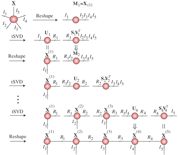
Figure 4.12: The TT-SVD algorithm for a 5th-order data tensor using truncated SVD. Instead of the SVD, any alternative LRMF algorithm can be employed, such as randomized SVD, RPCA, CUR/CA, NMF, SCA, ICA. Top panel: A 6th-order tensor $\underline{{\bf X}}$ of size $I_{1}\times I_{2}\times\cdots\times I_{5}$ is first reshaped into a long matrix ${\bf M}_{1}$ of size $I_{1}\times I_{2}\cdots I_{5}$. Second panel: The tSVD is performed to produce low-rank matrix factorization, with $I_{1}\times R_{1}$ factor matrix ${\bf U}_{1}$ and the $R_{1}\times I_{2}\cdots I_{5}$ matrix ${\bf S}_{1}{\bf V}_{1}^{\text{T}}$, so that ${\bf M}_{1}\cong{\bf U}_{1}{\bf S}_{1}{\bf V}_{1}^{\text{T}}$. Third panel: the matrix ${\bf U}_{1}$ becomes the first core core $\underline{{\bf X}}^{(1)}\in\mathbb{R}^{1\times I_{1}\times R_{1}}$, while the matrix ${\bf S}_{1}{\bf V}_{1}^{\text{T}}$ is reshaped into the $R_{1}I_{2}\times I_{3}I_{4}I_{5}$ matrix ${\bf M}_{2}$. Remaining panels: Perform tSVD to yield ${\bf M}_{2}\cong{\bf U}_{2}{\bf S}_{2}{\bf V}_{2}^{\text{T}}$, reshape ${\bf U}_{2}$ into an $R_{1}\times I_{2}\times R_{2}$ core $\underline{{\bf X}}^{(2)}$ and repeat the procedure until all the five cores are extracted (bottom panel). The same procedure applies to higher order tensors of any order.

The two basic approaches to perform efficiently TT decompositions are based on: (1) low-rank matrix factorizations (LRMF), and (2) constrained Tucker-2 decompositions.

4.7 Sequential SVD/LRMF Algorithms

The most important algorithm for the TT decomposition is the TT-SVD algorithm (see Algorithm 11) [216, 161], which applies the truncated SVD sequentially to the unfolding matrices, as illustrated in Figure 4.12. Instead of SVD, alternative and efficient LRMF algorithms can be used [50], see also Algorithm 12). For example, in [162] a new approximate formula for TT decomposition is proposed, where an $N$th-order data tensor $\underline{{\bf X}}$ is interpolated using a special form of cross-approximation. In fact, the TT-Cross-Approximation is analogous to the TT-SVD algorithm, but uses adaptive cross-approximation instead of the computationally more expensive SVD. The complexity of the cross-approximation algorithms scales linearly with the order $N$ of a data tensor.

0:  $N$th-order tensor $\underline{{\bf X}}\in\mathbb{R}^{I_{1}\times I_{2}\times\cdots\times I_{N}}$ and approximation accuracy $\varepsilon$ 0:  Approximative representation of a tensor in the TT format $\underline{\widehat{\bf X}}=\mathopen{\hbox{\set@color${\langle}$}\kern-1.94444pt\leavevmode\hbox{\set@color${\langle}$}}\underline{\widehat{\bf X}}^{(1)},\underline{\widehat{\bf X}}^{(2)},\ldots,\underline{\widehat{\bf X}}^{(N)}\mathclose{\hbox{\set@color${\rangle}$}\kern-1.94444pt\leavevmode\hbox{\set@color${\rangle}$}}$, such that $\|\underline{{\bf X}}-\underline{\widehat{\bf X}}\|_{F}\leq\varepsilon$ 1:  Unfolding of tensor $\underline{{\bf X}}$ in mode-1 ${\bf M}_{1}={\bf X}_{(1)}$ 2:  Initialization $R_{0}=1$ 3:  for $n=1$ to $N-1$ do 4:     Perform tSVD $[{\bf U}_{n},{\bf S}_{n},{\bf V}_{n}]=\mbox{tSVD}({\bf M}_{n},\varepsilon/\sqrt{N-1})$ 5:     Estimate $n$th TT rank $R_{n}=\mbox{size}({\bf U}_{n},2)$ 6:     Reshape orthogonal matrix ${\bf U}_{n}$ into a 3rd-order core $\underline{\widehat{\bf X}}^{(n)}=\mbox{reshape}({\bf U}_{n},[R_{n-1},I_{n},R_{n}])$ 7:     Reshape the matrix ${\bf V}_{n}$ into a matrix ${\bf M}_{n+1}=\mbox{reshape}\left({\bf S}_{n}{\bf V}_{n}^{\text{T}},[R_{n}I_{n+1},\prod_{p=n+2}^{N}I_{p}]\right)$ 8:  end for 9:  Construct the last core as $\underline{\widehat{\bf X}}^{(N)}=\mbox{reshape}({\bf M}_{N},[R_{N-1},I_{N},1])$ 10:  return  $\mathopen{\hbox{\set@color${\langle}$}\kern-1.94444pt\leavevmode\hbox{\set@color${\langle}$}}\underline{\widehat{\bf X}}^{(1)},\underline{\widehat{\bf X}}^{(2)},\ldots,\underline{\widehat{\bf X}}^{(N)}\mathclose{\hbox{\set@color${\rangle}$}\kern-1.94444pt\leavevmode\hbox{\set@color${\rangle}$}}$.

Algorithm 11 TT-SVD Decomposition using truncated SVD (tSVD) or randomized SVD (rSVD) [216, 158]

0:  Tensor $\underline{{\bf X}}\in\mathbb{R}^{I_{1}\times I_{2}\times\cdots\times I_{N}}$ and the approximation accuracy $\varepsilon$

0:  Approximate tensor representation in the TT format $\underline{\widehat{\bf X}}\cong\mathopen{\hbox{\set@color${\langle}$}\kern-1.94444pt\leavevmode\hbox{\set@color${\langle}$}}\underline{\widehat{\bf X}}^{(1)},\underline{\widehat{\bf X}}^{(2)},\ldots,\underline{\widehat{\bf X}}^{(N)}\mathclose{\hbox{\set@color${\rangle}$}\kern-1.94444pt\leavevmode\hbox{\set@color${\rangle}$}}$

1:  Initialization $R_{0}=1$

2:  Unfolding of tensor $\underline{{\bf X}}$ in mode-1 as ${\bf M}_{1}={\bf X}_{(1)}$

3:  for $n=1$ to $N-1$ do

4:     Perform LRMF, e.g., CUR, RPCA, …

$[{\bf A}_{n},{\bf B}_{n}]=\mbox{LRMF}({\bf M}_{n},\varepsilon)$, i.e., ${\bf M}_{n}\cong{\bf A}_{n}{\bf B}_{n}^{\text{T}}$

5:     Estimate $n$th TT rank, $R_{n}=\mbox{size}({\bf A}_{n},2)$

6:     Reshape matrix ${\bf A}_{n}$ into a 3rd-order core, as $\underline{\widehat{\bf X}}^{(n)}=\mbox{reshape}\left({\bf A}_{n},[R_{n-1},I_{n},R_{n}]\right)$

7:     Reshape the matrix ${\bf B}_{n}$ into the $(n+1)$th unfolding matrix ${\bf M}_{n+1}=\mbox{reshape}\left({\bf B}^{\text{T}}_{n},[R_{n}I_{n+1},\prod_{p=n+2}^{N}I_{p}]\right)$

8:  end for

9:  Construct the last core as $\underline{\widehat{\bf X}}^{(N)}=\mbox{reshape}({\bf M}_{N},[R_{N-1},I_{N},1])$

10:  return  TT-cores: $\mathopen{\hbox{\set@color${\langle}$}\kern-1.94444pt\leavevmode\hbox{\set@color${\langle}$}}\underline{\widehat{\bf X}}^{(1)},\underline{\widehat{\bf X}}^{(2)},\ldots,\underline{\widehat{\bf X}}^{(N)}\mathclose{\hbox{\set@color${\rangle}$}\kern-1.94444pt\leavevmode\hbox{\set@color${\rangle}$}}$.

Algorithm 12 TT Decomposition using any efficient LRMF

4.8 Tucker-2/PVD Algorithms for Large-scale TT Decompositions

(a)

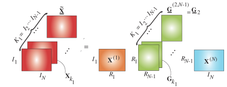
(b)

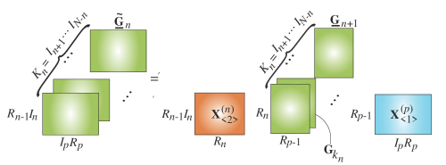
(c)

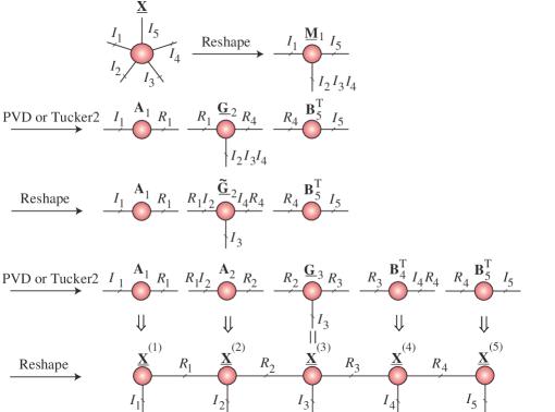
Figure 4.13: TT decomposition based on the Tucker-2/PVD model. (a) Extraction of the first and the last core. (b) The procedure can be repeated sequentially for reshaped 3rd-order tensors $\underline{{\bf G}}_{n}$ (for $n=2,3,\ldots$ and $p=N-1,N-2,\ldots$). (c) Illustration of a TT decomposition for a 5th-order data tensor, using an algorithm based on sequential Tucker-2/PVD decompositions.

The key idea in this approach is to reshape any $N$th-order data tensor, $\underline{{\bf X}}\in\mathbb{R}^{I_{1}\times I_{2}\times\cdots\times I_{N}}$ with $N>3$, into a suitable 3rd-order tensor, e.g., $\underline{\widetilde{\bf X}}\in\mathbb{R}^{I_{1}\;\times I_{N}\;\times\;I_{2}\cdots I_{N-1}}$, in order to apply the Tucker-2 decomposition as follows (see Algorithm 8 and Figure 4.13(a))

$$\underline{\widetilde{\bf X}}=\underline{{\bf G}}^{(2,N-1)}\times_{1}{\bf X}^{(1)}\times_{2}{\bf X}^{(N)}={\bf X}^{(1)}\times^{1}\underline{{\bf G}}^{(2,N-1)}\times^{1}{\bf X}^{(N)},$$ (4.34)

which, by using frontal slices of the involved tensors, can also be expressed in the matrix form

$${\bf X}_{k_{1}}={\bf X}^{(1)}{\bf G}_{k_{1}}{\bf X}^{(N)},\quad k_{1}=1,2,\ldots,I_{2}\cdots I_{N-1}.$$ (4.35)

Such representations allow us to compute the tensor, $\underline{{\bf G}}^{(2,N-1)}$, the first TT-core, ${\bf X}^{(1)}$, and the last TT-core, ${\bf X}^{(N)}$. The procedure can be repeated sequentially for reshaped tensors $\underline{\widetilde{{\bf G}}}_{n}=\underline{{\bf G}}^{(n+1,N-n)}$ for $n=1,2,\ldots$, in order to extract subsequent TT-cores in their matricized forms, as illustrated in Figure 4.13(b). See also the detailed step-by-step procedure shown in Figure 4.13(c).

Such a simple recursive procedure for TT decomposition can be used in conjunction with any efficient algorithm for Tucker-2/PVD decompositions or the nonnegative Tucker-2 decomposition (NTD-2) (see also Section 3).

4.9 Tensor Train Rounding – TT Recompression

0:  $N$th-order tensor $\underline{{\bf X}}=\mathopen{\hbox{\set@color${\langle}$}\kern-1.94444pt\leavevmode\hbox{\set@color${\langle}$}}\underline{{\bf X}}^{(1)},\underline{{\bf X}}^{(2)},\ldots,\underline{{\bf X}}^{(N)}\mathclose{\hbox{\set@color${\rangle}$}\kern-1.94444pt\leavevmode\hbox{\set@color${\rangle}$}}\in\mathbb{R}^{I_{1}\times I_{2}\times\cdots\times I_{N}}$,

in a TT format with an overestimated TT rank, ${\bf r}_{TT}=\{R_{1},R_{2},\ldots,R_{N-1}\}$, and TT-cores $\underline{{\bf X}}\in\mathbb{R}^{R_{n-1}\times I_{n}\times R_{n}}$,

absolute tolerance $\varepsilon$, and maximum rank $R_{\max}$

0:  $N$th-order tensor $\widehat{\underline{{\bf X}}}$ with a reduced TT rank; the cores are rounded (reduced) according to the input tolerance $\varepsilon$ and/or ranks bounded by $R_{\max}$, such that $\|\underline{{\bf X}}-\widehat{\underline{{\bf X}}}\|_{F}\leq\varepsilon\;\|\underline{{\bf X}}\|_{F}$

1:  Initialization $\underline{\widehat{\bf X}}=\underline{{\bf X}}$ and $\delta=\varepsilon/\sqrt{N-1}$

2:  for $n=1$ to $N-1$ do

3:     QR decomposition ${\bf X}^{(n)}_{<2>}={\bf Q}_{n}{\bf R}$, with ${\bf X}^{(n)}_{<2>}\in\mathbb{R}^{R_{n-1}I_{n}\times R_{n}}$

4:     Replace cores ${\bf X}^{(n)}_{<2>}={\bf Q}_{n}$ and ${\bf X}^{(n+1)}_{<1>}\leftarrow{\bf R}{\bf X}^{(n+1)}_{<1>}$, with ${\bf X}^{(n+1)}_{<1>}\in\mathbb{R}^{R_{n}\times I_{n+1}R_{n+1}}$

5:  end for

6:  for $n=N$ to $2$ do

7:     Perform $\delta$-truncated SVD ${\bf X}^{(n)}_{<1>}={\bf U}\mathop{\rm diag}\nolimits\{\mbox{\boldmath$\sigma$}\}{\bf V}^{\text{T}}$

8:     Determine minimum rank $\widehat{R}_{n-1}$ such that $\sum_{r>R_{n-1}}\sigma_{r}^{2}\leq\delta^{2}\|\mbox{\boldmath$\sigma$}\|^{2}$

9:     Replace cores ${\widehat{\bf X}}^{(n-1)}_{<2>}\leftarrow{\widehat{\bf X}}^{(n-1)}_{<2>}\widehat{\bf U}\mathop{\rm diag}\nolimits\{\widehat{\mbox{\boldmath$\sigma$}}\}$ and ${\widehat{\bf X}}^{(n)}_{<1>}=\widehat{\bf V}^{\text{T}}$

10:  end for

11:  return  $N$th-order tensor

$\widehat{{\bf X}}=\mathopen{\hbox{\set@color${\langle}$}\kern-1.94444pt\leavevmode\hbox{\set@color${\langle}$}}\widehat{\underline{{\bf X}}}^{(1)},\widehat{\underline{{\bf X}}}^{(2)},\ldots,\widehat{\underline{{\bf X}}}^{(N)}\mathclose{\hbox{\set@color${\rangle}$}\kern-1.94444pt\leavevmode\hbox{\set@color${\rangle}$}}\in\mathbb{R}^{I_{1}\times I_{2}\times\cdots\times I_{N}}$,

with reduced cores $\widehat{\underline{{\bf X}}}^{(n)}\in\mathbb{R}^{\widehat{R}_{n-1}\times I_{n}\times\widehat{R}_{n}}$

Algorithm 13 TT Rounding (Recompression) [158]

Mathematical operations in TT format produce core tensors with ranks which are not guaranteed to be optimal with respect to the desired approximation accuracy. For example, matrix-by-vector or matrix-by-matrix products considerably increase the TT ranks, which quickly become computationally prohibitive, so that a truncation or low-rank TT approximations are necessary for mathematical tractability. To this end, the TT–rounding (also called truncation or recompression) may be used as a post-processing procedure to reduce the TT ranks. The TT rounding algorithms are typically implemented via QR/SVD with the aim to approximate, with a desired prescribed accuracy, the TT core tensors, $\underline{{\bf G}}^{(n)}=\underline{{\bf X}}^{(n)}$, by other core tensors with minimum possible TT-ranks (see Algorithm 13). Note that TT rounding is mathematically the same as the TT-SVD, but is more efficient owing to the to use of TT format.

The complexity of TT-rounding procedures is only ${\cal{O}}(NIR^{3})$, since all operations are performed in TT format which requires the SVD to be computed only for a relatively small matricized core tensor at each iteration. A similar approach has been developed for the HT format [86, 87, 122, 74].

4.10 Orthogonalization of Tensor Train Network

The orthogonalization of core tensors is an essential procedure in many algorithms for the TT formats [158, 97, 70, 67, 120, 196, 197].

For convenience, we divide a TT network, which represents a tensor $\underline{\widehat{{\bf X}}}=\mathopen{\hbox{\set@color${\langle}$}\kern-1.94444pt\leavevmode\hbox{\set@color${\langle}$}}\underline{\widehat{{\bf X}}}^{(1)},\underline{\widehat{{\bf X}}}^{(2)},\ldots,\underline{\widehat{{\bf X}}}^{(N)}\mathclose{\hbox{\set@color${\rangle}$}\kern-1.94444pt\leavevmode\hbox{\set@color${\rangle}$}}\in\mathbb{R}^{I_{1}\times I_{2}\times\cdots\times I_{N}}$, into sub-trains. In this way, a large-scale task is replaced by easier-to-handle sub-tasks, whereby the aim is to extract a specific TT core or its slices from the whole TT network. For this purpose, the TT sub-trains can be defined as follows

$$\underline{\widehat{{\bf X}}}^{<n} = \mathopen{\hbox{\set@color${\langle}$}\kern-1.94444pt\leavevmode\hbox{\set@color${\langle}$}}\underline{\widehat{{\bf X}}}^{(1)},\underline{\widehat{{\bf X}}}^{(2)},\ldots,\underline{\widehat{{\bf X}}}^{(n-1)}\mathclose{\hbox{\set@color${\rangle}$}\kern-1.94444pt\leavevmode\hbox{\set@color${\rangle}$}}\in\mathbb{R}^{I_{1}\times I_{2}\times\cdots\times I_{n-1}\times R_{n-1}}$$ (4.36)

$$\underline{\widehat{{\bf X}}}^{>n} = \mathopen{\hbox{\set@color${\langle}$}\kern-1.94444pt\leavevmode\hbox{\set@color${\langle}$}}\underline{\widehat{{\bf X}}}^{(n+1)},\underline{\widehat{{\bf X}}}^{(n+2)},\ldots,\underline{\widehat{{\bf X}}}^{(N)}\mathclose{\hbox{\set@color${\rangle}$}\kern-1.94444pt\leavevmode\hbox{\set@color${\rangle}$}}\in\mathbb{R}^{R_{n}\times I_{n+1}\times\cdots\times I_{N}}$$ (4.37)

while the corresponding unfolding matrices, also called interface matrices, are defined by

$$\widehat{{\bf X}}^{\leq n}\in\mathbb{R}^{I_{1}I_{2}\cdots I_{n}\times R_{n}},\qquad\widehat{{\bf X}}^{>n}\in\mathbb{R}^{R_{n}\times I_{n+1}\cdots I_{N}}.$$ (4.38)

The left and right unfolding of the cores are defined as

$$\widehat{{\bf X}}_{L}^{(n)}=\widehat{{\bf X}}_{<2>}^{(n)}\in\mathbb{R}^{R_{n-1}I_{n}\times R_{n}}\;\;\mbox{and}\;\;\widehat{{\bf X}}_{R}^{(n)}={\bf X}_{<1>}^{(n)}\in\mathbb{R}^{R_{n-1}\times I_{n}R_{n}}\,.$$

0:  $N$th-order tensor $\underline{\widehat{{\bf X}}}=\mathopen{\hbox{\set@color${\langle}$}\kern-1.94444pt\leavevmode\hbox{\set@color${\langle}$}}\underline{\widehat{{\bf X}}}^{(1)},\underline{\widehat{{\bf X}}}^{(2)},\ldots,\underline{\widehat{{\bf X}}}^{(N)}\mathclose{\hbox{\set@color${\rangle}$}\kern-1.94444pt\leavevmode\hbox{\set@color${\rangle}$}}\in\mathbb{R}^{I_{1}\times I_{2}\times\cdots\times I_{N}}$,

with TT cores $\underline{\widehat{{\bf X}}}^{(n)}\in\mathbb{R}^{R_{n-1}\times I_{n}\times R_{n}}$ and $R_{0}=R_{N}=1$

0:  Cores $\underline{\widehat{{\bf X}}}^{(1)},\ldots,\underline{\widehat{{\bf X}}}^{(n-1)}$ become left-orthogonal, while the

remaining cores are right-orthogonal, except for the core $\underline{\widehat{{\bf X}}}^{(n)}$

1:  for $m=1$ to $n-1$ do

2:     Perform the QR decomposition $[{\bf Q},{\bf R}]\leftarrow qr({\widehat{{\bf X}}}^{(m)}_{L})$ for the

unfolding cores ${\widehat{{\bf X}}}^{(m)}_{L}\in\mathbb{R}^{R_{m-1}I_{m}\times R_{m}}$

3:     Replace the cores ${\widehat{{\bf X}}}^{(m)}_{L}\leftarrow{\bf Q}$ and $\underline{\widehat{{\bf X}}}^{(m+1)}\leftarrow\underline{\widehat{{\bf X}}}^{(m+1)}\times_{1}{\bf R}$

4:  end for

5:  for $m=N$ to $n+1$ do

6:     Perform QR decomposition $[{\bf Q},{\bf R}]\leftarrow qr(({\widehat{{\bf X}}}^{(m)}_{R})^{\text{T}})$ for the

unfolding cores $({\widehat{{\bf X}}}^{(m)}_{R})\in\mathbb{R}^{R_{m-1}\times I_{m}R_{m}}$,

7:     Replace the cores: ${\bf G}^{(m)}_{R}\leftarrow{\bf Q}^{\text{T}}$ and $\underline{\widehat{{\bf X}}}^{(m-1)}\leftarrow\underline{\widehat{{\bf X}}}^{(m-1)}\times_{3}{\bf R}^{\text{T}}$

8:  end for

9:  return  Left-orthogonal TT cores with $({\widehat{{\bf X}}}^{(m)}_{L})^{\text{T}}{\widehat{{\bf X}}}^{(m)}_{L}={\bf I}_{R_{m}}$ for $m=1,2,\ldots,n-1$ and right-orthogonal cores ${\widehat{{\bf X}}}^{(m)}_{R}({\widehat{{\bf X}}}^{(m)}_{R})^{\text{T}}={\bf I}_{R_{m-1}}$

for $m=N,N-1,\ldots,n+1$.

Algorithm 14 Left-orthogonalization, right-orthogonalization and $n$-orthogonalization of a tensor in the TT format

The $n$-orthogonality of tensors. An $N$th-order tensor in a TT format $\underline{\widehat{{\bf X}}}=\mathopen{\hbox{\set@color${\langle}$}\kern-1.94444pt\leavevmode\hbox{\set@color${\langle}$}}\underline{\widehat{{\bf X}}}^{(1)},\ldots,\underline{\widehat{{\bf X}}}^{(N)}\mathclose{\hbox{\set@color${\rangle}$}\kern-1.94444pt\leavevmode\hbox{\set@color${\rangle}$}}$, is called $n$-orthogonal with $1\leq n\leq N$, if

$$({\widehat{{\bf X}}}_{L}^{(m)})^{\text{T}}{\widehat{{\bf X}}}_{L}^{(m)}={\bf I}_{R_{m}},\;\;m=1,\ldots,n-1$$ (4.39)

$${\widehat{{\bf X}}}_{R}^{(m)}({\widehat{{\bf X}}}_{R}^{(m)})^{\text{T}}={\bf I}_{R_{m-1}},\;\;m=n+1,\ldots,N.$$ (4.40)

The tensor is called left-orthogonal if $n=N$ and right-orthogonal if $n=1$.

When considering the $n$th TT core, it is usually assumed that all cores to the left are left-orthogonalized, and all cores to the right are right-orthogonalized. Notice that if a TT tensor, $\underline{\widehat{{\bf X}}}$, is $n$-orthogonal then the “left” and “right” interface matrices have orthonormal columns and rows, that is

$$(\widehat{{\bf X}}^{<n})^{\text{T}}\;\widehat{{\bf X}}^{<n}={\bf I}_{R_{n-1}},\qquad\widehat{{\bf X}}^{>n}\;(\widehat{{\bf X}}^{>n})^{\text{T}}={\bf I}_{R_{n}}.$$ (4.41)

A tensor in a TT format can be orthogonalized efficiently using recursive QR and LQ decompositions (see Algorithm 14). From the above definition, for $n=N$ the algorithms perform left-orthogonalization and for $n=1$ right-orthogonalization of the whole TT network.

4.11 Improved TT Decomposition Algorithm – Alternating Single Core Update (ASCU)

Finally, we next present an efficient algorithm for TT decomposition, referred to as the Alternating Single Core Update (ASCU), which sequentially optimizes a single TT-core tensor while keeping the other TT-cores fixed in a manner similar to the modified ALS [170].

Assume that the TT-tensor $\underline{\widehat{{\bf X}}}=\mathopen{\hbox{\set@color${\langle}$}\kern-1.94444pt\leavevmode\hbox{\set@color${\langle}$}}\underline{\widehat{{\bf X}}}^{(1)},\underline{\widehat{{\bf X}}}^{(2)},\ldots,\underline{\widehat{{\bf X}}}^{(N)}\mathclose{\hbox{\set@color${\rangle}$}\kern-1.94444pt\leavevmode\hbox{\set@color${\rangle}$}}$ is left- and right-orthogonalized up to $\underline{\widehat{{\bf X}}}^{(n)}$, i.e., the unfolding matrices $\underline{\widehat{{\bf X}}}^{(k)}_{<2>}$ for $k=1,\ldots,n-1$ have orthonormal columns, and $\underline{\widehat{{\bf X}}}^{(m)}_{(1)}$ for $m=n+1,\ldots,N$ have orthonormal rows. Then, the Frobenius norm of the TT-tensor $\underline{\widehat{{\bf X}}}$ is equivalent to the Frobenius norm of $\underline{\widehat{{\bf X}}}^{(n)}$, that is, $\|\underline{\widehat{{\bf X}}}\|_{F}^{2}=\|\underline{\widehat{{\bf X}}}^{(n)}\|_{F}^{2}$, so that the Frobenius norm of the approximation error between a data tensor $\underline{{\bf X}}$ and its approximate representation in the TT format $\underline{\widehat{{\bf X}}}$ can be written as

$$J(\underline{{\bf X}}^{(n)}) = \|\underline{{\bf X}}-\underline{\widehat{{\bf X}}}\|_{F}^{2}$$

$$= \|\underline{{\bf X}}\|_{F}^{2}+\|\underline{\widehat{{\bf X}}}\|_{F}^{2}-2\langle\underline{{\bf X}},\;\underline{\widehat{{\bf X}}}\rangle$$

$$= \|\underline{{\bf X}}\|_{F}^{2}+\|\underline{\widehat{{\bf X}}}^{(n)}\|_{F}^{2}-2\langle\underline{{\bf C}}^{(n)},\;\underline{\widehat{{\bf X}}}^{(n)}\rangle$$

$$= \|\underline{{\bf X}}\|_{F}^{2}-\|\underline{{\bf C}}^{(n)}\|_{F}^{2}+\|\underline{{\bf C}}^{(n)}-\underline{\widehat{{\bf X}}}^{(n)}\|_{F}^{2},\qquad n=1,\ldots,N,$$

where $\underline{{\bf C}}^{(n)}\in\mathbb{R}^{R_{n-1}\times I_{n}\times R_{n}}$represents a tensor contraction of $\underline{{\bf X}}$ and $\underline{\widehat{{\bf X}}}$ along all modes but the mode-$n$, as illustrated in Figure 4.14. The $\underline{{\bf C}}^{(n)}$ can be efficiently computed through left contractions along the first $(n-1)$-modes and right contractions along the last $(N-m)$-modes, expressed as

$$\underline{{\bf L}}^{<n}=\underline{\widehat{{\bf X}}}^{<n}\,{\ltimes}_{n-1}\;\underline{{\bf X}},\qquad\underline{{\bf C}}^{(n)} = \underline{{\bf L}}^{<n}\,\rtimes_{N-n}\;\underline{\widehat{{\bf X}}}^{>n}.$$ (4.43)

The symbols $\ltimes_{n}$ and $\rtimes_{m}$ stand for the tensor contractions between two $N$th-order tensors along their first $n$ modes and last $m=N-n$ modes, respectively.

The optimization problem in (4.11) is usually performed subject to the following constraint

$$\|\underline{{\bf X}}-\underline{\widehat{{\bf X}}}\|_{F}^{2}\leq\varepsilon^{2}\,$$ (4.44)

such that the TT-rank of $\underline{\widehat{{\bf X}}}$ is minimum.

Observe that the constraint in (4.44) for left- and right-orthogonalized TT-cores is equivalent to the set of sub-constraints

$$\|\underline{{\bf C}}^{(n)}-\underline{\widehat{{\bf X}}}^{(n)}\|_{F}^{2}\leq\varepsilon_{n}^{2}\,\qquad n=1,\ldots,N,$$ (4.45)

whereby the $n$th core $\underline{{\bf X}}^{(n)}\in\mathbb{R}^{R_{n-1}\times I_{n}\times R_{n}}$ should have minimum ranks $R_{n-1}$ and $R_{n}$. Furthermore, $\varepsilon_{n}^{2}=\varepsilon^{2}-\|\underline{{\bf X}}\|_{F}^{2}+\|\underline{{\bf C}}^{(n)}\|_{F}^{2}$ is assumed to be non-negative. Finally, we can formulate the following sequential optimization problem

$$\min \left(R_{n-1}\cdot R_{n}\right),$$ (4.46)

s.t. $$\|\underline{{\bf C}}^{(n)}-\underline{\widehat{{\bf X}}}^{(n)}\|_{F}^{2}\leq\varepsilon_{n}^{2},\quad n=1,2,\ldots,N.$$

By expressing the TT-core tensor $\underline{\widehat{{\bf X}}}^{(n)}$ as a TT-tensor of three factors, i.e., in a Tucker-2 format given by

$$\underline{\widehat{{\bf X}}}^{(n)}={\bf A}_{n}\times^{1}\tilde{\underline{{\bf X}}}^{(n)}\times^{1}{\bf B}_{n}\,,$$

the above optimization problem with the constraint (4.45) reduces to performing a Tucker-2 decomposition (see Algorithm 8). The aim is to compute ${\bf A}_{n}$, ${\bf B}_{n}$ (orthogonal factor matrices) and a core tensor $\tilde{\underline{{\bf X}}}^{(n)}$ which approximates tensor $\underline{{\bf C}}^{(n)}$ with a minimum TT-rank-$(\tilde{R}_{n-1},\tilde{R}_{n})$, such that

$$\|\underline{{\bf C}}^{(n)}-{\bf A}_{n}\times^{1}\tilde{\underline{{\bf X}}}^{(n)}\times^{1}{\bf B}_{n}\|_{F}^{2}\leq\varepsilon_{n}^{2}\,,$$

where ${\bf A}_{n}\in\mathbb{R}^{R_{n-1}\times\tilde{R}_{n-1}}$ and ${\bf B}_{n}\in\mathbb{R}^{\tilde{R}_{n}\times R_{n}}$, with $\tilde{R}_{n-1}\leftarrow R_{n-1}$ and $\tilde{R}_{n}\leftarrow R_{n}$.

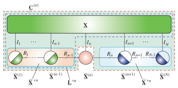
Figure 4.14: Illustration of the contraction of tensors in the Alternating Single Core Update (ASCU) algorithm (see Algorithm 15). All the cores to the left of $\underline{{\bf X}}^{(n)}$ are left-orthogonal and all cores to its right are right-orthogonal.

Note that the new estimate of $\underline{{\bf X}}$ is still of $N$th-order because the factor matrices ${\bf A}_{n}$ and ${\bf B}_{n}$ can be embedded into $\underline{\widehat{{\bf X}}}^{(n-1)}$ and $\underline{\widehat{{\bf X}}}^{(n+1)}$ as follows

$$\underline{\widehat{{\bf X}}} =\underline{\widehat{{\bf X}}}^{(1)}\times^{1}\cdots\times^{1}(\underline{\widehat{{\bf X}}}^{(n-1)}\times^{1}{\bf A}_{n})\times^{1}\tilde{\underline{{\bf X}}}^{(n)}\times^{1}({\bf B}_{n}\times^{1}\underline{\widehat{{\bf X}}}^{(n+1)})$$

$$\quad\times^{1}\cdots\times^{1}\underline{\widehat{{\bf X}}}^{(N)}\,.$$

In this way, the three TT-cores $\underline{\widehat{{\bf X}}}^{(n-1)}$, $\underline{\widehat{{\bf X}}}^{(n)}$ and $\underline{\widehat{{\bf X}}}^{(n+1)}$ are updated. Since ${\bf A}_{n}$ and ${\bf B}_{n}^{\text{T}}$ have respectively orthonormal columns and rows, the newly adjusted cores $(\underline{\widehat{{\bf X}}}^{(n-1)}\times^{1}{\bf A}_{n})$ and $({\bf B}_{n}\times^{1}\underline{\widehat{{\bf X}}}^{(n+1)})$ obey the left- and right-orthogonality conditions. Algorithm 15 outlines such a single-core update algorithm based on the Tucker-2 decomposition. In the pseudo-code, the left contracted tensor $\underline{{\bf L}}^{<n}$ is computed efficiently through a progressive contraction in the form [182, 101]

$$\underline{{\bf L}}^{<n} = \underline{\widehat{\bf X}}^{(n-1)}\ltimes_{2}\;\underline{{\bf L}}^{<(n-1)},$$ (4.47)

where $\underline{{\bf L}}^{<1}=\underline{{\bf X}}$.

0:  Data tensor $\underline{{\bf X}}\in\mathbb{R}^{I_{1}\times I_{2}\times\cdots\times I_{N}}$ and approximation accuracy $\varepsilon$ 0:  TT-tensor $\underline{\widehat{{\bf X}}}=\underline{\widehat{{\bf X}}}^{(1)}\times^{1}\underline{\widehat{{\bf X}}}^{(2)}\times^{1}\cdots\times^{1}\underline{\widehat{{\bf X}}}^{(N)}$ of minimum TT-rank such that $\|\underline{{\bf X}}-\underline{\widehat{{\bf X}}}\|_{F}^{2}\leq\varepsilon^{2}$ 1:  Initialize $\underline{\widehat{{\bf X}}}=\mathopen{\hbox{\set@color${\langle}$}\kern-1.94444pt\leavevmode\hbox{\set@color${\langle}$}}\underline{\widehat{{\bf X}}}^{(1)},\underline{\widehat{{\bf X}}}^{(2)},\ldots,\underline{\widehat{{\bf X}}}^{(N)}\mathclose{\hbox{\set@color${\rangle}$}\kern-1.94444pt\leavevmode\hbox{\set@color${\rangle}$}}$ 2:  repeat 3:     for $n=1,2,\ldots,N-1$ do 4:        Compute contracted tensor $\underline{{\bf C}}^{(n)}=\underline{{\bf L}}^{<n}\rtimes_{N-n}\;\underline{\widehat{{\bf X}}}^{>n}$ 5:        Solve a Tucker-2 decomposition $\|\underline{{\bf C}}^{(n)}-{\bf A}_{n}\times^{1}\underline{\widehat{{\bf X}}}^{(n)}\times^{1}{\bf B}_{n}\|_{F}^{2}\leq\varepsilon^{2}-\|\underline{{\bf X}}\|_{F}^{2}+\|\underline{{\bf C}}^{(n)}\|_{F}^{2}$ 6:        Adjust adjacent cores $\underline{\widehat{\bf X}}^{(n-1)}\leftarrow\underline{\widehat{\bf X}}^{(n-1)}\times^{1}{\bf A}_{n}$, $\qquad\underline{\widehat{{\bf X}}}^{(n+1)}\leftarrow{\bf B}_{n}\times^{1}\underline{\widehat{{\bf X}}}^{(n+1)}$ 7:        Perform left-orthogonalization of $\underline{\widehat{{\bf X}}}^{(n)}$ 8:        Update left-side contracted tensors $\underline{{\bf L}}^{<n}\leftarrow{\bf A}_{n}^{\text{T}}\times^{1}\underline{{\bf L}}^{<n}$, $\qquad\underline{{\bf L}}^{<(n+1)}\leftarrow\underline{\widehat{{\bf X}}}^{(n)}\ltimes_{2}\;\underline{{\bf L}}^{<n}$ 9:     end for 10:     for $n=N,N-1,\ldots,2$ do 11:        Compute contracted tensor $\underline{{\bf C}}^{(n)}=\underline{{\bf L}}^{<n}\rtimes_{N-n}\;\underline{\widehat{{\bf X}}}^{>n}$ 12:        Solve a constrained Tucker-2 decomposition $\|\underline{{\bf C}}^{(n)}-{\bf A}_{n}\times^{1}\underline{\widehat{{\bf X}}}^{(n)}\times^{1}{\bf B}_{n}\|_{F}^{2}\leq\varepsilon^{2}-\|\underline{{\bf X}}\|_{F}^{2}+\|\underline{{\bf C}}^{(n)}\|_{F}^{2}$ 13:        $\underline{\widehat{\bf X}}^{(n-1)}\leftarrow\underline{\widehat{{\bf X}}}^{(n-1)}\times^{1}{\bf A}_{n}$, $\qquad\underline{\widehat{{\bf X}}}^{(n+1)}\leftarrow{\bf B}_{n}\times^{1}\underline{\widehat{{\bf X}}}^{(n+1)}$ 14:        Perform right-orthogonalization of $\underline{\widehat{{\bf X}}}^{(n)}$ 15:     end for 16:  until a stopping criterion is met 17:  return  $\mathopen{\hbox{\set@color${\langle}$}\kern-1.94444pt\leavevmode\hbox{\set@color${\langle}$}}\underline{\widehat{\bf X}}^{(1)},\underline{\widehat{\bf X}}^{(2)},\ldots,\underline{\widehat{\bf X}}^{(N)}\mathclose{\hbox{\set@color${\rangle}$}\kern-1.94444pt\leavevmode\hbox{\set@color${\rangle}$}}$.

Algorithm 15 The Alternating Single-Core Update Algorithm (two-sides rank adjustment) [170]

0:  Data tensor $\underline{{\bf X}}\in\mathbb{R}^{I_{1}\times I_{2}\times\cdots\times I_{N}}$ and approximation accuracy $\varepsilon$ 0:  TT-tensor $\underline{\widehat{{\bf X}}}=\underline{\widehat{{\bf X}}}^{(1)}\times^{1}\underline{\widehat{{\bf X}}}^{(2)}\times^{1}\cdots\times^{1}\underline{\widehat{{\bf X}}}^{(N)}$ of minimum TT-rank such that $\|\underline{{\bf X}}-\underline{\widehat{{\bf X}}}\|_{F}^{2}\leq\varepsilon^{2}$ 1:  Initialize TT-cores $\underline{\widehat{{\bf X}}}^{(n)},\quad\forall n$ 2:  repeat 3:     for $n=1,2,\ldots,N-1$ do 4:        Compute the contracted tensor $\underline{{\bf C}}^{(n)}=\underline{{\bf L}}^{<n}\rtimes_{N-n}\;\underline{\widehat{{\bf X}}}^{>n}$ 5:        Truncated SVD: $\|[\underline{{\bf C}}^{(n)}]_{<2>}-{\bf U}\,\mbox{\boldmath$\Sigma$}\,{\bf V}^{\text{T}}\|_{F}^{2}\leq\varepsilon^{2}-\|\underline{{\bf X}}\|_{F}^{2}+\|\underline{{\bf C}}^{(n)}\|_{F}^{2}$ 6:        Update $\underline{\widehat{{\bf X}}}^{(n)}=\text{reshape}({\bf U},R_{n-1}\times I_{n}\times R_{n})$ 7:        Adjust adjacent core $\underline{\widehat{{\bf X}}}^{(n+1)}\leftarrow(\mbox{\boldmath$\Sigma$}\,{\bf V}^{\text{T}})\times^{1}\underline{\widehat{{\bf X}}}^{(n+1)}$ 8:        Update left-side contracted tensors $\underline{{\bf L}}^{<(n+1)}\leftarrow\underline{\widehat{{\bf X}}}^{(n)}\ltimes_{2}\;\underline{{\bf L}}^{<n}$ 9:     end for 10:     for $n=N,N-1,\ldots,2$ do 11:        Compute contracted tensor $\underline{{\bf C}}^{(n)}=\underline{{\bf L}}^{<n}\rtimes_{N-n}\;\underline{\widehat{{\bf X}}}^{>n}$ 12:        Truncated SVD: $\|[\underline{{\bf C}}^{(n)}]_{(1)}-{\bf U}\,\mbox{\boldmath$\Sigma$}\,{\bf V}^{\text{T}}\|_{F}^{2}\leq\varepsilon^{2}-\|\underline{{\bf X}}\|_{F}^{2}+\|\underline{{\bf C}}^{(n)}\|_{F}^{2}$; 13:        $\underline{\widehat{{\bf X}}}^{(n)}=\text{reshape}({\bf V}^{\text{T}},R_{n-1}\times I_{n}\times R_{n})$ 14:        $\underline{\widehat{{\bf X}}}^{(n-1)}\leftarrow\underline{\widehat{{\bf X}}}^{(n-1)}\times^{1}({\bf U}\,\mbox{\boldmath$\Sigma$})$ 15:     end for 16:  until a stopping criterion is met 17:  return  $\mathopen{\hbox{\set@color${\langle}$}\kern-1.94444pt\leavevmode\hbox{\set@color${\langle}$}}\underline{\widehat{\bf X}}^{(1)},\underline{\widehat{\bf X}}^{(2)},\ldots,\underline{\widehat{\bf X}}^{(N)}\mathclose{\hbox{\set@color${\rangle}$}\kern-1.94444pt\leavevmode\hbox{\set@color${\rangle}$}}$.

Algorithm 16 The Alternating Single-Core Update Algorithm (one-side rank adjustment) [170]

Alternatively, instead of adjusting the two TT ranks, $R_{n-1}$ and $R_{n}$, of $\underline{\widehat{{\bf X}}}^{(n)}$, we can update only one rank, either $R_{n-1}$ or $R_{n}$, corresponding to the right-to-left or left-to-right update order procedure. Assuming that the core tensors are updated in the left-to-right order, we need to find $\underline{\widehat{{\bf X}}}^{(n)}$ which has a minimum rank-$R_{n}$ and satisfies the constraints

$$\|\underline{{\bf C}}^{(n)}-\underline{\widehat{{\bf X}}}^{(n)}\;\times^{1}\;{\bf B}_{n}\|_{F}^{2}\leq\varepsilon_{n}^{2},\qquad n=1,\ldots,N.$$

This problem reduces to the truncated SVD of the mode-$\{1,2\}$ matricization of $\underline{{\bf C}}^{(n)}$ with an accuracy $\varepsilon_{n}^{2}$, that is

$$[\underline{{\bf C}}^{(n)}]_{<2>}\approx{\bf U}_{n}\,\mbox{\boldmath$\Sigma$}\,{\bf V}_{n}^{\text{T}}\,,$$

where $\mbox{\boldmath$\Sigma$}=\mathop{\rm diag}\nolimits(\sigma_{n,1},\ldots,\sigma_{n,R_{n}^{\star}})$. Here, for the new optimized rank $R_{n}^{\star}$, the following holds

$$\sum_{r=1}^{R_{n}^{\star}}\,\sigma_{n,r}^{2}\geq\|\underline{{\bf X}}\|_{F}^{2}-\varepsilon^{2}>\sum_{r=1}^{R_{n}^{\star}-1}\,\sigma_{n,r}^{2}\,.$$ (4.48)

The core tensor $\underline{\widehat{{\bf X}}}^{(n)}$ is then updated by reshaping ${\bf U}_{n}$ to an order-3 tensor of size $R_{n-1}\times I_{n}\times R_{n}^{\star}$, while the core $\underline{\widehat{{\bf X}}}^{(n+1)}$ needs to be adjusted accordingly as

$$\underline{\widehat{{\bf X}}}^{(n+1)\star}=\mbox{\boldmath$\Sigma$}\,{\bf V}_{n}^{\text{T}}\times^{1}\underline{\widehat{{\bf X}}}^{(n+1)}\,.$$ (4.49)

When the algorithm updates the core tensors in the right-to-left order, we update $\underline{\widehat{{\bf X}}}^{(n)}$ by using the $R_{n-1}^{\star}$ leading right singular vectors of the mode-1 matricization of $\underline{{\bf C}}^{(n)}$, and adjust the core $\underline{\widehat{{\bf X}}}^{(n-1)}$ accordingly, that is,

$$[\underline{{\bf C}}^{(n)}]_{(1)} \cong{\bf U}_{n}\,\mbox{\boldmath$\Sigma$}\,{\bf V}_{n}^{\text{T}}\,$$

$$\underline{\widehat{{\bf X}}}^{(n)\star} =\text{reshape}({\bf V}_{n}^{\text{T}},[R_{n-1}^{\star},I_{n},R_{n}])$$

$$\underline{\widehat{{\bf X}}}^{(n-1)\star} =\underline{\widehat{{\bf X}}}^{(n-1)}\times^{1}({\bf U}_{n}\,\mbox{\boldmath$\Sigma$})\,.$$ (4.50)

To summarise, the ASCU method performs a sequential update of one core and adjusts (or rotates) another core. Hence, it updates two cores at a time (for detail see Algorithm 16).

The ASCU algorithm can be implemented in an even more efficient way, if the data tensor $\underline{{\bf X}}$ is already given in a TT format (with a non-optimal TT ranks for the prescribed accuracy). Detailed MATLAB implementations and other variants of the TT decomposition algorithm are provided in [170].

Chapter 5 Discussion and Conclusions

In Part 1 of this monograph, we have provided a systematic and example-rich guide to the basic properties and applications of tensor network methodologies, and have demonstrated their promise as a tool for the analysis of extreme-scale multidimensional data. Our main aim has been to illustrate that, owing to the intrinsic compression ability that stems from the distributed way in which they represent data and process information, TNs can be naturally employed for linear/multilinear dimensionality reduction. Indeed, current applications of TNs include generalized multivariate regression, compressed sensing, multi-way blind source separation, sparse representation and coding, feature extraction, classification, clustering and data fusion.

With multilinear algebra as their mathematical backbone, TNs have been shown to have intrinsic advantages over the flat two-dimensional view provided by matrices, including the ability to model both strong and weak couplings among multiple variables, and to cater for multimodal, incomplete and noisy data.

In Part 2 of this monograph we introduce a scalable framework for distributed implementation of optimization algorithms, in order to transform huge-scale optimization problems into linked small-scale optimization sub-problems of the same type. In that sense, TNs can be seen as a natural bridge between small-scale and very large-scale optimization paradigms, which allows for any efficient standard numerical algorithm to be applied to such local optimization sub-problems.

Although research on tensor networks for dimensionality reduction and optimization problems is only emerging, given that in many modern applications, multiway arrays (tensors) arise, either explicitly or indirectly, through the tensorization of vectors and matrices, we foresee this material serving as a useful foundation for further studies on a variety of machine learning problems for data of otherwise prohibitively large volume, variety, or veracity. We also hope that the readers will find the approaches presented in this monograph helpful in advancing seamlessly from numerical linear algebra to numerical multilinear algebra.

References

- [1] E. Acar and B. Yener. Unsupervised multiway data analysis: A literature survey. IEEE Transactions on Knowledge and Data Engineering, 21:6–20, 2009.
- [2] I. Affleck, T. Kennedy, E.H. Lieb, and H. Tasaki. Rigorous results on valence-bond ground states in antiferromagnets. Physical Review Letters, 59(7):799, 1987.
- [3] A. Anandkumar, R. Ge, D. Hsu, S.M. Kakade, and M. Telgarsky. Tensor decompositions for learning latent variable models. Journal of Machine Learning Research, 15:2773–2832, 2014.
- [4] D. Anderson, S. Du, M. Mahoney, C. Melgaard, K. Wu, and M. Gu. Spectral gap error bounds for improving CUR matrix decomposition and the Nyström method. In Proceedings of the 18th International Conference on Artificial Intelligence and Statistics, pages 19–27, 2015.
- [5] W. Austin, G. Ballard, and T.G. Kolda. Parallel tensor compression for large-scale scientific data. arXiv preprint arXiv:1510.06689, 2015.
- [6] F.R. Bach and M.I. Jordan. Kernel independent component analysis. The Journal of Machine Learning Research, 3:1–48, 2003.
- [7] M. Bachmayr, R. Schneider, and A. Uschmajew. Tensor networks and hierarchical tensors for the solution of high-dimensional partial differential equations. Foundations of Computational Mathematics, 16(6):1423–1472, 2016.
- [8] B.W. Bader and T.G. Kolda. MATLAB tensor toolbox version 2.6, February 2015.
- [9] J. Ballani and L. Grasedyck. Tree adaptive approximation in the hierarchical tensor format. SIAM Journal on Scientific Computing, 36(4):A1415–A1431, 2014.
- [10] J. Ballani, L. Grasedyck, and M. Kluge. A review on adaptive low-rank approximation techniques in the hierarchical tensor format. In Extraction of Quantifiable Information from Complex Systems, pages 195–210. Springer, 2014.
- [11] G. Ballard, A.R. Benson, A. Druinsky, B. Lipshitz, and O. Schwartz. Improving the numerical stability of fast matrix multiplication algorithms. arXiv preprint arXiv:1507.00687, 2015.
- [12] G. Ballard, A. Druinsky, N. Knight, and O. Schwartz. Brief announcement: Hypergraph partitioning for parallel sparse matrix-matrix multiplication. In Proceedings of the 27th ACM on Symposium on Parallelism in Algorithms and Architectures, pages 86–88. ACM, 2015.
- [13] G. Barcza, Ö. Legeza, K.H. Marti, and M. Reiher. Quantum-information analysis of electronic states of different molecular structures. Physical Review A, 83(1):012508, 2011.
- [14] K. Batselier, H. Liu, and N. Wong. A constructive algorithm for decomposing a tensor into a finite sum of orthonormal rank-1 terms. SIAM Journal on Matrix Analysis and Applications, 36(3):1315–1337, 2015.
- [15] K. Batselier and N. Wong. A constructive arbitrary-degree Kronecker product decomposition of tensors. arXiv preprint arXiv:1507.08805, 2015.
- [16] M. Bebendorf. Adaptive cross-approximation of multivariate functions. Constructive Approximation, 34(2):149–179, 2011.
- [17] M. Bebendorf, C. Kuske, and R. Venn. Wideband nested cross approximation for Helmholtz problems. Numerische Mathematik, 130(1):1–34, 2015.
- [18] R.E. Bellman. Adaptive Control Processes. Princeton University Press, Princeton, NJ, 1961.
- [19] P. Benner, V. Khoromskaia, and B.N. Khoromskij. A reduced basis approach for calculation of the Bethe–Salpeter excitation energies by using low-rank tensor factorisations. Molecular Physics, 114(7-8):1148–1161, 2016.
- [20] A.R. Benson, J.D. Lee, B. Rajwa, and D.F. Gleich. Scalable methods for nonnegative matrix factorizations of near-separable tall-and-skinny matrices. In Proceedings of Neural Information Processing Systems (NIPS), pages 945–953, 2014.
- [21] D. Bini. Tensor and border rank of certain classes of matrices and the fast evaluation of determinant inverse matrix and eigenvalues. Calcolo, 22(1):209–228, 1985.
- [22] M. Bolten, K. Kahl, and S. Sokolović. Multigrid Methods for Tensor Structured Markov Chains with Low Rank Approximation. SIAM Journal on Scientific Computing, 38(2):A649–A667, 2016.
- [23] S. Boyd, N. Parikh, E. Chu, B. Peleato, and J. Eckstein. Distributed optimization and statistical learning via the alternating direction method of multipliers. Foundations and Trends in Machine Learning, 3(1):1–122, 2011.
- [24] A. Bruckstein, D. Donoho, and M. Elad. From sparse solutions of systems of equations to sparse modeling of signals and images. SIAM Review, 51(1):34–81, 2009.
- [25] H.-J. Bungartz and M. Griebel. Sparse grids. Acta Numerica, 13:147–269, 2004.
- [26] C. Caiafa and A. Cichocki. Generalizing the column-row matrix decomposition to multi-way arrays. Linear Algebra and its Applications, 433(3):557–573, 2010.
- [27] C. Caiafa and A Cichocki. Computing sparse representations of multidimensional signals using Kronecker bases. Neural Computaion, 25(1):186–220, 2013.
- [28] C. Caiafa and A. Cichocki. Stable, robust, and super–fast reconstruction of tensors using multi-way projections. IEEE Transactions on Signal Processing, 63(3):780–793, 2015.
- [29] J.D. Carroll and J.-J. Chang. Analysis of individual differences in multidimensional scaling via an N-way generalization of ”Eckart-Young” decomposition. Psychometrika, 35(3):283–319, 1970.
- [30] V. Cevher, S. Becker, and M. Schmidt. Convex optimization for big data: Scalable, randomized, and parallel algorithms for big data analytics. IEEE Signal Processing Magazine, 31(5):32–43, 2014.
- [31] G. Chabriel, M. Kleinsteuber, E. Moreau, H. Shen, P. Tichavsky, and A. Yeredor. Joint matrix decompositions and blind source separation: A survey of methods, identification, and applications. IEEE Signal Processing Magazine, 31(3):34–43, 2014.
- [32] V. Chandola, A. Banerjee, and V. Kumar. Anomaly detection: A survey. ACM Computing Surveys (CSUR), 41(3):15, 2009.
- [33] T.-L. Chen, D. D. Chang, S.-Y. Huang, H. Chen, C. Lin, and W. Wang. Integrating multiple random sketches for singular value decomposition. arXiv e-prints, 2016.
- [34] H. Cho, D. Venturi, and G.E. Karniadakis. Numerical methods for high-dimensional probability density function equations. Journal of Computational Physics, 305:817–837, 2016.
- [35] J.H. Choi and S. Vishwanathan. DFacTo: Distributed factorization of tensors. In Advances in Neural Information Processing Systems, pages 1296–1304, 2014.
- [36] W. Chu and Z. Ghahramani. Probabilistic models for incomplete multi-dimensional arrays. In JMLR Workshop and Conference Proceedings Volume 5: AISTATS 2009, volume 5, pages 89–96. Microtome Publishing (paper) Journal of Machine Learning Research, 2009.
- [37] A. Cichocki. Era of big data processing: A new approach via tensor networks and tensor decompositions, (invited). In Proceedings of the International Workshop on Smart Info-Media Systems in Asia (SISA2013), September 2013.
- [38] A. Cichocki. Tensor decompositions: A new concept in brain data analysis? arXiv preprint arXiv:1305.0395, 2013.
- [39] A. Cichocki. Tensor networks for big data analytics and large-scale optimization problems. arXiv preprint arXiv:1407.3124, 2014.
- [40] A. Cichocki and S. Amari. Adaptive Blind Signal and Image Processing: Learning Algorithms and Applications. John Wiley & Sons, Ltd, 2003.
- [41] A. Cichocki, S. Cruces, and S. Amari. Log-determinant divergences revisited: Alpha-beta and gamma log-det divergences. Entropy, 17(5):2988–3034, 2015.
- [42] A. Cichocki, D. Mandic, C. Caiafa, A.H. Phan, G. Zhou, Q. Zhao, and L. De Lathauwer. Tensor decompositions for signal processing applications: From two-way to multiway component analysis. IEEE Signal Processing Magazine, 32(2):145–163, 2015.
- [43] A. Cichocki, R Zdunek, A.-H. Phan, and S. Amari. Nonnegative Matrix and Tensor Factorizations: Applications to Exploratory Multi-way Data Analysis and Blind Source Separation. Wiley, Chichester, 2009.
- [44] N. Cohen, O. Sharir, and A. Shashua. On the expressive power of deep learning: A tensor analysis. In 29th Annual Conference on Learning Theory, pages 698–728, 2016.
- [45] N. Cohen and A. Shashua. Convolutional rectifier networks as generalized tensor decompositions. In Proceedings of The 33rd International Conference on Machine Learning, pages 955–963, 2016.
- [46] P. Comon. Tensors: a brief introduction. IEEE Signal Processing Magazine, 31(3):44–53, 2014.
- [47] P. Comon and C. Jutten. Handbook of Blind Source Separation: Independent Component Analysis and Applications. Academic Press, 2010.
- [48] P.G. Constantine and D.F. Gleich. Tall and skinny QR factorizations in MapReduce architectures. In Proceedings of the Second International Workshop on MapReduce and its Applications, pages 43–50. ACM, 2011.
- [49] P.G. Constantine, D.F Gleich, Y. Hou, and J. Templeton. Model reduction with MapReduce-enabled tall and skinny singular value decomposition. SIAM Journal on Scientific Computing, 36(5):S166–S191, 2014.
- [50] E. Corona, A. Rahimian, and D. Zorin. A Tensor-Train accelerated solver for integral equations in complex geometries. arXiv preprint arXiv:1511.06029, November 2015.
- [51] C. Crainiceanu, B. Caffo, S. Luo, V. Zipunnikov, and N. Punjabi. Population value decomposition, a framework for the analysis of image populations. Journal of the American Statistical Association, 106(495):775–790, 2011.
- [52] A. Critch and J. Morton. Algebraic geometry of matrix product states. Symmetry, Integrability and Geometry: Methods and Applications (SIGMA), 10:095, 2014.
- [53] A.J. Critch. Algebraic Geometry of Hidden Markov and Related Models. PhD thesis, University of California, Berkeley, 2013.
- [54] A.L.F. de Almeida, G. Favier, J.C.M. Mota, and J.P.C.L. da Costa. Overview of tensor decompositions with applications to communications. In R.F. Coelho, V.H. Nascimento, R.L. de Queiroz, J.M.T. Romano, and C.C. Cavalcante, editors, Signals and Images: Advances and Results in Speech, Estimation, Compression, Recognition, Filtering, and Processing, chapter 12, pages 325–355. CRC Press, 2015.
- [55] F. De la Torre. A least-squares framework for component analysis. IEEE Transactions on Pattern Analysis and Machine Intelligence, 34(6):1041–1055, 2012.
- [56] L. De Lathauwer. A link between the canonical decomposition in multilinear algebra and simultaneous matrix diagonalization. SIAM Journal on Matrix Analysis and Applications, 28:642–666, 2006.
- [57] L. De Lathauwer. Decompositions of a higher-order tensor in block terms — Part I and II. SIAM Journal on Matrix Analysis and Applications, 30(3):1022–1066, 2008. Special Issue on Tensor Decompositions and Applications.
- [58] L. De Lathauwer. Blind separation of exponential polynomials and the decomposition of a tensor in rank- terms. SIAM Journal on Matrix Analysis and Applications, 32(4):1451–1474, 2011.
- [59] L. De Lathauwer, B. De Moor, and J. Vandewalle. A Multilinear Singular Value Decomposition. SIAM Journal on Matrix Analysis Applications, 21:1253–1278, 2000.
- [60] L. De Lathauwer, B. De Moor, and J. Vandewalle. On the best rank-1 and rank- approximation of higher-order tensors. SIAM Journal of Matrix Analysis and Applications, 21(4):1324–1342, 2000.
- [61] L. De Lathauwer and D. Nion. Decompositions of a higher-order tensor in block terms – Part III: Alternating least squares algorithms. SIAM Journal on Matrix Analysis and Applications, 30(3):1067–1083, 2008.
- [62] W. de Launey and J. Seberry. The strong Kronecker product. Journal of Combinatorial Theory, Series A, 66(2):192–213, 1994.
- [63] V. de Silva and L.-H. Lim. Tensor rank and the ill-posedness of the best low-rank approximation problem. SIAM Journal on Matrix Analysis and Applications, 30:1084–1127, 2008.
- [64] A. Desai, M. Ghashami, and J.M. Phillips. Improved practical matrix sketching with guarantees. IEEE Transactions on Knowledge and Data Engineering, 28(7):1678–1690, 2016.
- [65] I.S. Dhillon. Fast Newton-type methods for nonnegative matrix and tensor approximation. The NSF Workshop, Future Directions in Tensor-Based Computation and Modeling, 2009.
- [66] E. Di Napoli, D. Fabregat-Traver, G. Quintana-Ortí, and P. Bientinesi. Towards an efficient use of the BLAS library for multilinear tensor contractions. Applied Mathematics and Computation, 235:454–468, 2014.
- [67] S.V. Dolgov. Tensor Product Methods in Numerical Simulation of High-dimensional Dynamical Problems. PhD thesis, Faculty of Mathematics and Informatics, University Leipzig, Germany, Leipzig, Germany, 2014.
- [68] S.V. Dolgov and B.N. Khoromskij. Two-level QTT-Tucker format for optimized tensor calculus. SIAM Journal on Matrix Analysis and Applications, 34(2):593–623, 2013.
- [69] S.V. Dolgov and B.N. Khoromskij. Simultaneous state-time approximation of the chemical master equation using tensor product formats. Numerical Linear Algebra with Applications, 22(2):197–219, 2015.
- [70] S.V. Dolgov, B.N. Khoromskij, I.V. Oseledets, and D.V. Savostyanov. Computation of extreme eigenvalues in higher dimensions using block tensor train format. Computer Physics Communications, 185(4):1207–1216, 2014.
- [71] S.V. Dolgov and D.V. Savostyanov. Alternating minimal energy methods for linear systems in higher dimensions. SIAM Journal on Scientific Computing, 36(5):A2248–A2271, 2014.
- [72] P. Drineas and M.W. Mahoney. A randomized algorithm for a tensor-based generalization of the singular value decomposition. Linear Algebra and its Applications, 420(2):553–571, 2007.
- [73] G. Ehlers, J. Sólyom, Ö. Legeza, and R.M. Noack. Entanglement structure of the hubbard model in momentum space. Physical Review B, 92(23):235116, 2015.
- [74] M Espig, M Schuster, A Killaitis, N Waldren, P Wähnert, S Handschuh, and H Auer. TensorCalculus library, 2012.
- [75] F. Esposito, T. Scarabino, A. Hyvärinen, J. Himberg, E. Formisano, S. Comani, G. Tedeschi, R. Goebel, E. Seifritz, and F. Di Salle. Independent component analysis of fMRI group studies by self-organizing clustering. NeuroImage, 25(1):193–205, 2005.
- [76] G. Evenbly and G. Vidal. Algorithms for entanglement renormalization. Physical Review B, 79(14):144108, 2009.
- [77] G. Evenbly and S. R. White. Entanglement Renormalization and Wavelets. Physical Review Letters, 116(14):140403, 2016.
- [78] H. Fanaee-T and J. Gama. Tensor-based anomaly detection: An interdisciplinary survey. Knowledge-Based Systems, 2016.
- [79] G. Favier and A. de Almeida. Overview of constrained PARAFAC models. EURASIP Journal on Advances in Signal Processing, 2014(1):1–25, 2014.
- [80] J. Garcke, M. Griebel, and M. Thess. Data mining with sparse grids. Computing, 67(3):225–253, 2001.
- [81] S. Garreis and M. Ulbrich. Constrained optimization with low-rank tensors and applications to parametric problems with PDEs. SIAM Journal on Scientific Computing, (accepted), 2016.
- [82] M. Ghashami, E. Liberty, and J.M. Phillips. Efficient frequent directions algorithm for sparse matrices. arXiv preprint arXiv:1602.00412, 2016.
- [83] V. Giovannetti, S. Montangero, and R. Fazio. Quantum multiscale entanglement renormalization ansatz channels. Physical Review Letters, 101(18):180503, 2008.
- [84] S.A. Goreinov, E.E. Tyrtyshnikov, and N.L. Zamarashkin. A theory of pseudo-skeleton approximations. Linear Algebra and its Applications, 261:1–21, 1997.
- [85] S.A. Goreinov, N.L. Zamarashkin, and E.E. Tyrtyshnikov. Pseudo-skeleton approximations by matrices of maximum volume. Mathematical Notes, 62(4):515–519, 1997.
- [86] L. Grasedyck. Hierarchical singular value decomposition of tensors. SIAM Journal on Matrix Analysis and Applications, 31(4):2029–2054, 2010.
- [87] L. Grasedyck, D. Kessner, and C. Tobler. A literature survey of low-rank tensor approximation techniques. GAMM-Mitteilungen, 36:53–78, 2013.
- [88] A.R. Groves, C.F. Beckmann, S.M. Smith, and M.W. Woolrich. Linked independent component analysis for multimodal data fusion. NeuroImage, 54(1):2198 – 21217, 2011.
- [89] Z.-C. Gu, M. Levin, B. Swingle, and X.-G. Wen. Tensor-product representations for string-net condensed states. Physical Review B, 79(8):085118, 2009.
- [90] M. Haardt, F. Roemer, and G. Del Galdo. Higher-order SVD based subspace estimation to improve the parameter estimation accuracy in multi-dimensional harmonic retrieval problems. IEEE Transactions on Signal Processing, 56:3198–3213, July 2008.
- [91] W. Hackbusch. Tensor Spaces and Numerical Tensor Calculus, volume 42 of Springer Series in Computational Mathematics. Springer, Heidelberg, 2012.
- [92] W. Hackbusch and S. Kühn. A new scheme for the tensor representation. Journal of Fourier Analysis and Applications, 15(5):706–722, 2009.
- [93] N. Halko, P. Martinsson, and J. Tropp. Finding structure with randomness: Probabilistic algorithms for constructing approximate matrix decompositions. SIAM Review, 53(2):217–288, 2011.
- [94] S. Handschuh. Numerical Methods in Tensor Networks. PhD thesis, Facualty of Mathematics and Informatics, University Leipzig, Germany, Leipzig, Germany, 2015.
- [95] R.A. Harshman. Foundations of the PARAFAC procedure: Models and conditions for an explanatory multimodal factor analysis. UCLA Working Papers in Phonetics, 16:1–84, 1970.
- [96] F.L. Hitchcock. Multiple invariants and generalized rank of a -way matrix or tensor. Journal of Mathematics and Physics, 7:39–79, 1927.
- [97] S. Holtz, T. Rohwedder, and R. Schneider. The alternating linear scheme for tensor optimization in the tensor train format. SIAM Journal on Scientific Computing, 34(2), 2012.
- [98] M. Hong, M. Razaviyayn, Z.Q. Luo, and J.S. Pang. A unified algorithmic framework for block-structured optimization involving big data with applications in machine learning and signal processing. IEEE Signal Processing Magazine, 33(1):57–77, 2016.
- [99] H. Huang, C. Ding, D. Luo, and T. Li. Simultaneous tensor subspace selection and clustering: The equivalence of high order SVD and K-means clustering. In Proceedings of the 14th ACM SIGKDD International Conference on Knowledge Discovery and Data mining, pages 327–335. ACM, 2008.
- [100] R. Hübener, V. Nebendahl, and W. Dür. Concatenated tensor network states. New Journal of Physics, 12(2):025004, 2010.
- [101] C. Hubig, I.P. McCulloch, U. Schollwöck, and F.A. Wolf. Strictly single-site DMRG algorithm with subspace expansion. Physical Review B, 91(15):155115, 2015.
- [102] T. Huckle, K. Waldherr, and T. Schulte-Herbriggen. Computations in quantum tensor networks. Linear Algebra and its Applications, 438(2):750 – 781, 2013.
- [103] A. Hyvärinen. Independent component analysis: Recent advances. Philosophical Transactions of the Royal Society A, 371(1984):20110534, 2013.
- [104] I. Jeon, E.E. Papalexakis, C. Faloutsos, L. Sael, and U. Kang. Mining billion-scale tensors: Algorithms and discoveries. The VLDB Journal, pages 1–26, 2016.
- [105] B. Jiang, F. Yang, and S. Zhang. Tensor and its Tucker core: The invariance relationships. arXiv e-prints arXiv:1601.01469, January 2016.
- [106] U. Kang, E.E. Papalexakis, A. Harpale, and C. Faloutsos. GigaTensor: Scaling tensor analysis up by 100 times - algorithms and discoveries. In Proceedings of the 18th ACM SIGKDD International Conference on Knowledge Discovery and Data Mining (KDD ’12), pages 316–324, August 2012.
- [107] Y.-J. Kao, Y.-D. Hsieh, and P. Chen. Uni10: An open-source library for tensor network algorithms. In Journal of Physics: Conference Series, volume 640, page 012040. IOP Publishing, 2015.
- [108] L. Karlsson, D. Kressner, and A. Uschmajew. Parallel algorithms for tensor completion in the CP format. Parallel Computing, 57:222–234, 2016.
- [109] J.-P. Kauppi, J. Hahne, K.R. Müller, and A. Hyvärinen. Three-way analysis of spectrospatial electromyography data: Classification and interpretation. PloS One, 10(6):e0127231, 2015.
- [110] V.A. Kazeev, M. Khammash, M. Nip, and C. Schwab. Direct solution of the chemical master equation using quantized tensor trains. PLoS Computational Biology, 10(3):e1003359, 2014.
- [111] V.A. Kazeev and B.N. Khoromskij. Low-rank explicit QTT representation of the Laplace operator and its inverse. SIAM Journal on Matrix Analysis and Applications, 33(3):742–758, 2012.
- [112] V.A. Kazeev, B.N. Khoromskij, and E.E. Tyrtyshnikov. Multilevel Toeplitz matrices generated by tensor-structured vectors and convolution with logarithmic complexity. SIAM Journal on Scientific Computing, 35(3):A1511–A1536, 2013.
- [113] V.A. Kazeev, O. Reichmann, and C. Schwab. Low-rank tensor structure of linear diffusion operators in the TT and QTT formats. Linear Algebra and its Applications, 438(11):4204–4221, 2013.
- [114] B.N. Khoromskij. -quantics approximation of - tensors in high-dimensional numerical modeling. Constructive Approximation, 34(2):257–280, 2011.
- [115] B.N. Khoromskij. Tensors-structured numerical methods in scientific computing: Survey on recent advances. Chemometrics and Intelligent Laboratory Systems, 110(1):1–19, 2011.
- [116] B.N. Khoromskij and A. Veit. Efficient computation of highly oscillatory integrals by using QTT tensor approximation. Computational Methods in Applied Mathematics, 16(1):145–159, 2016.
- [117] H.-J. Kim, E. Ollila, V. Koivunen, and H.V. Poor. Robust iteratively reweighted Lasso for sparse tensor factorizations. In IEEE Workshop on Statistical Signal Processing (SSP), pages 420–423, 2014.
- [118] S. Klus and C. Schütte. Towards tensor-based methods for the numerical approximation of the Perron-Frobenius and Koopman operator. arXiv e-prints arXiv:1512.06527, December 2015.
- [119] T.G. Kolda and B.W. Bader. Tensor decompositions and applications. SIAM Review, 51(3):455–500, 2009.
- [120] D. Kressner, M. Steinlechner, and A. Uschmajew. Low-rank tensor methods with subspace correction for symmetric eigenvalue problems. SIAM Journal on Scientific Computing, 36(5):A2346–A2368, 2014.
- [121] D. Kressner, M. Steinlechner, and B. Vandereycken. Low-rank tensor completion by Riemannian optimization. BIT Numerical Mathematics, 54(2):447–468, 2014.
- [122] D. Kressner and C. Tobler. Algorithm 941: HTucker–A MATLAB toolbox for tensors in hierarchical Tucker format. ACM Transactions on Mathematical Software, 40(3):22, 2014.
- [123] D. Kressner and A. Uschmajew. On low-rank approximability of solutions to high-dimensional operator equations and eigenvalue problems. Linear Algebra and its Applications, 493:556–572, 2016.
- [124] P.M. Kroonenberg. Applied Multiway Data Analysis. John Wiley & Sons Ltd, New York, 2008.
- [125] J.B. Kruskal. Three-way arrays: Rank and uniqueness of trilinear decompositions, with application to arithmetic complexity and statistics. Linear Algebra and its Applications, 18(2):95–138, 1977.
- [126] V. Kuleshov, A.T. Chaganty, and P. Liang. Tensor factorization via matrix factorization. In Proceedings of the Eighteenth International Conference on Artificial Intelligence and Statistics, pages 507–516, 2015.
- [127] N. Lee and A. Cichocki. Estimating a few extreme singular values and vectors for large-scale matrices in Tensor Train format. SIAM Journal on Matrix Analysis and Applications, 36(3):994–1014, 2015.
- [128] N. Lee and A. Cichocki. Fundamental tensor operations for large-scale data analysis using tensor network formats. Multidimensional Systems and Signal Processing, (accepted), 2016.
- [129] N. Lee and A. Cichocki. Regularized computation of approximate pseudoinverse of large matrices using low-rank tensor train decompositions. SIAM Journal on Matrix Analysis and Applications, 37(2):598–623, 2016.
- [130] N. Lee and A. Cichocki. Tensor train decompositions for higher order regression with LASSO penalties. In Workshop on Tensor Decompositions and Applications (TDA2016), 2016.
- [131] J. Li, C. Battaglino, I. Perros, J. Sun, and R. Vuduc. An input-adaptive and in-place approach to dense tensor-times-matrix multiply. In Proceedings of the International Conference for High Performance Computing, Networking, Storage and Analysis, page 76. ACM, 2015.
- [132] M. Li and V. Monga. Robust video hashing via multilinear subspace projections. IEEE Transactions on Image Processing, 21(10):4397–4409, 2012.
- [133] S. Liao, T. Vejchodský, and R. Erban. Tensor methods for parameter estimation and bifurcation analysis of stochastic reaction networks. Journal of the Royal Society Interface, 12(108):20150233, 2015.
- [134] A.P. Liavas and N.D. Sidiropoulos. Parallel algorithms for constrained tensor factorization via alternating direction method of multipliers. IEEE Transactions on Signal Processing, 63(20):5450–5463, 2015.
- [135] L.H. Lim and P. Comon. Multiarray signal processing: Tensor decomposition meets compressed sensing. Comptes Rendus Mecanique, 338(6):311–320, 2010.
- [136] M.S. Litsarev and I.V. Oseledets. A low-rank approach to the computation of path integrals. Journal of Computational Physics, 305:557–574, 2016.
- [137] H. Lu, K.N. Plataniotis, and A.N. Venetsanopoulos. A survey of multilinear subspace learning for tensor data. Pattern Recognition, 44(7):1540–1551, 2011.
- [138] M. Lubasch, J.I. Cirac, and M.-C. Banuls. Unifying projected entangled pair state contractions. New Journal of Physics, 16(3):033014, 2014.
- [139] C. Lubich, T. Rohwedder, R. Schneider, and B. Vandereycken. Dynamical approximation of hierarchical Tucker and tensor-train tensors. SIAM Journal on Matrix Analysis and Applications, 34(2):470–494, 2013.
- [140] M.W. Mahoney. Randomized algorithms for matrices and data. Foundations and Trends in Machine Learning, 3(2):123–224, 2011.
- [141] M.W. Mahoney and P. Drineas. CUR matrix decompositions for improved data analysis. Proceedings of the National Academy of Sciences, 106:697–702, 2009.
- [142] M.W. Mahoney, M. Maggioni, and P. Drineas. Tensor-CUR decompositions for tensor-based data. SIAM Journal on Matrix Analysis and Applications, 30(3):957–987, 2008.
- [143] H. Matsueda. Analytic optimization of a MERA network and its relevance to quantum integrability and wavelet. arXiv preprint arXiv:1608.02205, 2016.
- [144] A.Y. Mikhalev and I.V. Oseledets. Iterative representing set selection for nested cross–approximation. Numerical Linear Algebra with Applications, 2015.
- [145] L. Mirsky. Symmetric gauge functions and unitarily invariant norms. The Quarterly Journal of Mathematics, 11:50–59, 1960.
- [146] J. Morton. Tensor networks in algebraic geometry and statistics. Lecture at Networking Tensor Networks, Centro de Ciencias de Benasque Pedro Pascual, Benasque, Spain, 2012.
- [147] M. Mørup. Applications of tensor (multiway array) factorizations and decompositions in data mining. Wiley Interdisciplinary Review: Data Mining and Knowledge Discovery, 1(1):24–40, 2011.
- [148] V. Murg, F. Verstraete, R. Schneider, P.R. Nagy, and O. Legeza. Tree tensor network state with variable tensor order: An efficient multireference method for strongly correlated systems. Journal of Chemical Theory and Computation, 11(3):1027–1036, 2015.
- [149] N Nakatani and G.K.L. Chan. Efficient tree tensor network states (TTNS) for quantum chemistry: Generalizations of the density matrix renormalization group algorithm. The Journal of Chemical Physics, 2013.
- [150] Y. Nesterov. Efficiency of coordinate descent methods on huge-scale optimization problems. SIAM Journal on Optimization, 22(2):341–362, 2012.
- [151] Y. Nesterov. Subgradient methods for huge-scale optimization problems. Mathematical Programming, 146(1-2):275–297, 2014.
- [152] N. H. Nguyen, P. Drineas, and T. D. Tran. Tensor sparsification via a bound on the spectral norm of random tensors. Information and Inference, page iav004, 2015.
- [153] M. Nickel, K. Murphy, V. Tresp, and E. Gabrilovich. A review of relational machine learning for knowledge graphs. Proceedings of the IEEE, 104(1):11–33, 2016.
- [154] A. Novikov and R.A. Rodomanov. Putting MRFs on a tensor train. In Proceedings of the International Conference on Machine Learning (ICML ’14), 2014.
- [155] A.C. Olivieri. Analytical advantages of multivariate data processing. One, two, three, infinity? Analytical Chemistry, 80(15):5713–5720, 2008.
- [156] R. Orús. A practical introduction to tensor networks: Matrix product states and projected entangled pair states. Annals of Physics, 349:117–158, 2014.
- [157] I.V. Oseledets. Approximation of matrices using tensor decomposition. SIAM Journal on Matrix Analysis and Applications, 31(4):2130–2145, 2010.
- [158] I.V. Oseledets. Tensor-train decomposition. SIAM Journal on Scientific Computing, 33(5):2295–2317, 2011.
- [159] I.V. Oseledets and S.V. Dolgov. Solution of linear systems and matrix inversion in the TT-format. SIAM Journal on Scientific Computing, 34(5):A2718–A2739, 2012.
- [160] I.V. Oseledets, S.V. Dolgov, V.A. Kazeev, D. Savostyanov, O. Lebedeva, P. Zhlobich, T. Mach, and L. Song. TT-Toolbox, 2012.
- [161] I.V. Oseledets and E.E. Tyrtyshnikov. Breaking the curse of dimensionality, or how to use SVD in many dimensions. SIAM Journal on Scientific Computing, 31(5):3744–3759, 2009.
- [162] I.V. Oseledets and E.E. Tyrtyshnikov. TT cross–approximation for multidimensional arrays. Linear Algebra and its Applications, 432(1):70–88, 2010.
- [163] E.E. Papalexakis, C. Faloutsos, and N.D. Sidiropoulos. Tensors for data mining and data fusion: Models, applications, and scalable algorithms. ACM Transactions on Intelligent Systems and Technology (TIST), 8(2):16, 2016.
- [164] E.E. Papalexakis, N. Sidiropoulos, and R. Bro. From K-means to higher-way co-clustering: Multilinear decomposition with sparse latent factors. IEEE Transactions on Signal Processing, 61(2):493–506, 2013.
- [165] N. Parikh and S.P. Boyd. Proximal algorithms. Foundations and Trends in Optimization, 1(3):127–239, 2014.
- [166] D. Perez-Garcia, F. Verstraete, M.M. Wolf, and J.I. Cirac. Matrix product state representations. Quantum Information & Computation, 7(5):401–430, July 2007.
- [167] R. Pfeifer, G. Evenbly, S. Singh, and G. Vidal. NCON: A tensor network contractor for MATLAB. arXiv preprint arXiv:1402.0939, 2014.
- [168] N. Pham and R. Pagh. Fast and scalable polynomial kernels via explicit feature maps. In Proceedings of the 19th ACM SIGKDD international conference on Knowledge discovery and data mining, pages 239–247. ACM, 2013.
- [169] A-H. Phan and A. Cichocki. Extended HALS algorithm for nonnegative Tucker decomposition and its applications for multiway analysis and classification. Neurocomputing, 74(11):1956–1969, 2011.
- [170] A.-H. Phan, A. Cichocki, A. Uschmajew, P. Tichavsky, G. Luta, and D. Mandic. Tensor networks for latent variable analysis. Part I: Algorithms for tensor train decomposition. ArXiv e-prints, 2016.
- [171] A.-H. Phan, P. Tichavskỳ, and A. Cichocki. Fast alternating ls algorithms for high order candecomp/parafac tensor factorizations. IEEE Transactions on Signal Processing, 61(19):4834–4846, 2013.
- [172] A.-H. Phan, P. Tichavskỳ, and A. Cichocki. Tensor deflation for candecomp/parafac—part i: Alternating subspace update algorithm. IEEE Transactions on Signal Processing, 63(22):5924–5938, 2015.
- [173] A.H. Phan and A. Cichocki. Tensor decompositions for feature extraction and classification of high dimensional datasets. Nonlinear Theory and its Applications, IEICE, 1(1):37–68, 2010.
- [174] A.H. Phan, A. Cichocki, P. Tichavsky, D. Mandic, and K. Matsuoka. On revealing replicating structures in multiway data: A novel tensor decomposition approach. In Proceedings of the 10th International Conference LVA/ICA, Tel Aviv, March 12-15, pages 297–305. Springer, 2012.
- [175] A.H. Phan, A. Cichocki, P. Tichavský, R. Zdunek, and S.R. Lehky. From basis components to complex structural patterns. In Proceedings of the IEEE International Conference on Acoustics, Speech and Signal Processing, ICASSP 2013, Vancouver, BC, Canada, May 26-31, 2013, pages 3228–3232, 2013.
- [176] A.H. Phan, P. Tichavský, and A. Cichocki. Low complexity damped Gauss-Newton algorithms for CANDECOMP/PARAFAC. SIAM Journal on Matrix Analysis and Applications (SIMAX), 34(1):126–147, 2013.
- [177] A.H. Phan, P. Tichavský, and A. Cichocki. Low rank tensor deconvolution. In Proceedings of the IEEE International Conference on Acoustics Speech and Signal Processing, ICASSP, pages 2169–2173, April 2015.
- [178] S. Ragnarsson. Structured Tensor Computations: Blocking Symmetries and Kronecker Factorization. PhD dissertation, Cornell University, Department of Applied Mathematics, 2012.
- [179] M.V. Rakhuba and I.V. Oseledets. Fast multidimensional convolution in low-rank tensor formats via cross–approximation. SIAM Journal on Scientific Computing, 37(2):A565–A582, 2015.
- [180] P. Richtárik and M. Takáč. Parallel coordinate descent methods for big data optimization. Mathematical Programming, 156:433–484, 2016.
- [181] J. Salmi, A. Richter, and V. Koivunen. Sequential unfolding SVD for tensors with applications in array signal processing. IEEE Transactions on Signal Processing, 57:4719–4733, 2009.
- [182] U. Schollwöck. The density-matrix renormalization group in the age of matrix product states. Annals of Physics, 326(1):96–192, 2011.
- [183] U. Schollwöck. Matrix product state algorithms: DMRG, TEBD and relatives. In Strongly Correlated Systems, pages 67–98. Springer, 2013.
- [184] N. Schuch, I. Cirac, and D. Pérez-García. PEPS as ground states: Degeneracy and topology. Annals of Physics, 325(10):2153–2192, 2010.
- [185] N. Sidiropoulos, R. Bro, and G. Giannakis. Parallel factor analysis in sensor array processing. IEEE Transactions on Signal Processing, 48(8):2377–2388, 2000.
- [186] N.D. Sidiropoulos. Generalizing Caratheodory’s uniqueness of harmonic parameterization to N dimensions. IEEE Transactions on Information Theory, 47(4):1687–1690, 2001.
- [187] N.D. Sidiropoulos. Low-rank decomposition of multi-way arrays: A signal processing perspective. In Proceedings of the IEEE Sensor Array and Multichannel Signal Processing Workshop (SAM 2004), July 2004.
- [188] N.D. Sidiropoulos and R. Bro. On the uniqueness of multilinear decomposition of N-way arrays. Journal of Chemometrics, 14(3):229–239, 2000.
- [189] N.D. Sidiropoulos, L. De Lathauwer, X. Fu, K. Huang, E.E. Papalexakis, and C. Faloutsos. Tensor decomposition for signal processing and machine learning. arXiv e-prints arXiv:1607.01668, 2016.
- [190] A. Smilde, R. Bro, and P. Geladi. Multi-way Analysis: Applications in the Chemical Sciences. John Wiley & Sons Ltd, New York, 2004.
- [191] S.M. Smith, A. Hyvärinen, G. Varoquaux, K.L. Miller, and C.F. Beckmann. Group-PCA for very large fMRI datasets. NeuroImage, 101:738–749, 2014.
- [192] L. Sorber, I. Domanov, M. Van Barel, and L. De Lathauwer. Exact line and plane search for tensor optimization. Computational Optimization and Applications, 63(1):121–142, 2016.
- [193] L. Sorber, M. Van Barel, and L. De Lathauwer. Optimization-based algorithms for tensor decompositions: Canonical Polyadic Decomposition, decomposition in rank- terms and a new generalization. SIAM Journal on Optimization, 23(2), 2013.
- [194] M. Sørensen and L. De Lathauwer. Blind signal separation via tensor decomposition with Vandermonde factor. Part I: Canonical polyadic decomposition. IEEE Transactions on Signal Processing, 61(22):5507–5519, 2013.
- [195] M. Sørensen, L. De Lathauwer, P. Comon, S. Icart, and L. Deneire. Canonical Polyadic Decomposition with orthogonality constraints. SIAM Journal on Matrix Analysis and Applications, 33(4):1190–1213, 2012.
- [196] M. Steinlechner. Riemannian optimization for high-dimensional tensor completion. Technical report, Technical report MATHICSE 5.2015, EPF Lausanne, Switzerland, 2015.
- [197] M.M. Steinlechner. Riemannian Optimization for Solving High-Dimensional Problems with Low-Rank Tensor Structure. PhD thesis, École Polytechnnque Fédérale de Lausanne, 2016.
- [198] E.M. Stoudenmire and Steven R. White. Minimally entangled typical thermal state algorithms. New Journal of Physics, 12(5):055026, 2010.
- [199] J. Sun, D. Tao, and C. Faloutsos. Beyond streams and graphs: Dynamic tensor analysis. In Proceedings of the 12th ACM SIGKDD international conference on Knowledge Discovery and Data Mining, pages 374–383. ACM, 2006.
- [200] S.K. Suter, M. Makhynia, and R. Pajarola. TAMRESH - tensor approximation multiresolution hierarchy for interactive volume visualization. Computer Graphics Forum, 32(3):151–160, 2013.
- [201] Y. Tang, R. Salakhutdinov, and G. Hinton. Tensor analyzers. In Proceedings of the 30th International Conference on Machine Learning, (ICML 2013), Atlanta, USA, 2013.
- [202] D. Tao, X. Li, X. Wu, and S. Maybank. General tensor discriminant analysis and Gabor features for gait recognition. IEEE Transactions on Pattern Analysis and Machine Intelligence, 29(10):1700–1715, 2007.
- [203] P. Tichavsky and A. Yeredor. Fast approximate joint diagonalization incorporating weight matrices. IEEE Transactions on Signal Processing, 47(3):878–891, 2009.
- [204] M.K. Titsias. Variational learning of inducing variables in sparse Gaussian processes. In Proceedings of the 12th International Conference on Artificial Intelligence and Statistics, pages 567–574, 2009.
- [205] C. Tobler. Low-rank tensor methods for linear systems and eigenvalue problems. PhD thesis, ETH Zürich, 2012.
- [206] L.N. Trefethen. Cubature, approximation, and isotropy in the hypercube. SIAM Review (to appear), 2017.
- [207] V. Tresp, Y. Esteban, C.and Yang, S. Baier, and D. Krompaß. Learning with memory embeddings. arXiv preprint arXiv:1511.07972, 2015.
- [208] J. A. Tropp, A. Yurtsever, M. Udell, and V. Cevher. Randomized single-view algorithms for low-rank matrix approximation. arXiv e-prints, 2016.
- [209] L. Tucker. Some mathematical notes on three-mode factor analysis. Psychometrika, 31(3):279–311, 1966.
- [210] L.R. Tucker. The extension of factor analysis to three-dimensional matrices. In H. Gulliksen and N. Frederiksen, editors, Contributions to Mathematical Psychology, pages 110–127. Holt, Rinehart and Winston, New York, 1964.
- [211] A. Uschmajew and B. Vandereycken. The geometry of algorithms using hierarchical tensors. Linear Algebra and its Applications, 439:133—166, 2013.
- [212] N. Vannieuwenhoven, R. Vandebril, and K. Meerbergen. A new truncation strategy for the higher-order singular value decomposition. SIAM Journal on Scientific Computing, 34(2):A1027–A1052, 2012.
- [213] M.A.O. Vasilescu and D. Terzopoulos. Multilinear analysis of image ensembles: Tensorfaces. In Proceedings of the European Conference on Computer Vision (ECCV), volume 2350, pages 447–460, Copenhagen, Denmark, May 2002.
- [214] F. Verstraete, V. Murg, and I. Cirac. Matrix product states, projected entangled pair states, and variational renormalization group methods for quantum spin systems. Advances in Physics, 57(2):143–224, 2008.
- [215] N. Vervliet, O. Debals, L. Sorber, and L. De Lathauwer. Breaking the curse of dimensionality using decompositions of incomplete tensors: Tensor-based scientific computing in big data analysis. IEEE Signal Processing Magazine, 31(5):71–79, 2014.
- [216] G. Vidal. Efficient classical simulation of slightly entangled quantum computations. Physical Review Letters, 91(14):147902, 2003.
- [217] S.A. Vorobyov, Y. Rong, N.D. Sidiropoulos, and A.B. Gershman. Robust iterative fitting of multilinear models. IEEE Transactions on Signal Processing, 53(8):2678–2689, 2005.
- [218] S. Wahls, V. Koivunen, H.V. Poor, and M. Verhaegen. Learning multidimensional Fourier series with tensor trains. In IEEE Global Conference on Signal and Information Processing (GlobalSIP), pages 394–398. IEEE, 2014.
- [219] D. Wang, H. Shen, and Y. Truong. Efficient dimension reduction for high-dimensional matrix-valued data. Neurocomputing, 190:25–34, 2016.
- [220] H. Wang and M. Thoss. Multilayer formulation of the multiconfiguration time-dependent Hartree theory. Journal of Chemical Physics, 119(3):1289–1299, 2003.
- [221] H. Wang, Q. Wu, L. Shi, Y. Yu, and N. Ahuja. Out-of-core tensor approximation of multi-dimensional matrices of visual data. ACM Transactions on Graphics, 24(3):527–535, 2005.
- [222] S. Wang and Z. Zhang. Improving CUR matrix decomposition and the Nyström approximation via adaptive sampling. The Journal of Machine Learning Research, 14(1):2729–2769, 2013.
- [223] Y. Wang, H.-Y. Tung, A. Smola, and A. Anandkumar. Fast and guaranteed tensor decomposition via sketching. In Advances in Neural Information Processing Systems, pages 991–999, 2015.
- [224] S.R. White. Density-matrix algorithms for quantum renormalization groups. Physical Review B, 48(14):10345, 1993.
- [225] Z. Xu, F. Yan, and Y. Qi. Infinite Tucker decomposition: Nonparametric Bayesian models for multiway data analysis. In Proceedings of the 29th International Conference on Machine Learning (ICML), ICML ’12, pages 1023–1030. Omnipress, July 2012.
- [226] Y. Yang and T. Hospedales. Deep multi-task representation learning: A tensor factorisation approach. arXiv preprint arXiv:1605.06391, 2016.
- [227] T. Yokota, N. Lee, and A. Cichocki. Robust multilinear tensor rank estimation using Higher Order Singular Value Decomposition and Information Criteria. IEEE Transactions on Signal Processing, accepted, 2017.
- [228] T. Yokota, Q. Zhao, and A. Cichocki. Smooth PARAFAC decomposition for tensor completion. IEEE Transactions on Signal Processing, 64(20):5423–5436, 2016.
- [229] Z. Zhang, X. Yang, I.V. Oseledets, G.E. Karniadakis, and L. Daniel. Enabling high-dimensional hierarchical uncertainty quantification by ANOVA and tensor-train decomposition. IEEE Transactions on Computer-Aided Design of Integrated Circuits and Systems, 34(1):63–76, 2015.
- [230] H.H. Zhao, Z.Y. Xie, Q.N. Chen, Z.C. Wei, J.W. Cai, and T. Xiang. Renormalization of tensor-network states. Physical Review B, 81(17):174411, 2010.
- [231] Q. Zhao, C. Caiafa, D.P. Mandic, Z.C. Chao, Y. Nagasaka, N. Fujii, L. Zhang, and A. Cichocki. Higher order partial least squares (HOPLS): A generalized multilinear regression method. IEEE Transactions on Pattern Analysis and Machine Intelligence, 35(7):1660–1673, 2013.
- [232] Q. Zhao, G. Zhou, T. Adali, L. Zhang, and A. Cichocki. Kernelization of tensor-based models for multiway data analysis: Processing of multidimensional structured data. IEEE Signal Processing Magazine, 30(4):137–148, 2013.
- [233] S. Zhe, Y. Qi, Y. Park, Z. Xu, I. Molloy, and S. Chari. DinTucker: Scaling up Gaussian process models on large multidimensional arrays. In Proceedings of the Thirtieth AAAI Conference on Artificial Intelligence, 2016.
- [234] G. Zhou and A. Cichocki. Canonical Polyadic Decomposition based on a single mode blind source separation. IEEE Signal Processing Letters, 19(8):523–526, 2012.
- [235] G. Zhou and A. Cichocki. Fast and unique Tucker decompositions via multiway blind source separation. Bulletin of Polish Academy of Science, 60(3):389–407, 2012.
- [236] G. Zhou, A. Cichocki, and S. Xie. Fast nonnegative matrix/tensor factorization based on low-rank approximation. IEEE Transactions on Signal Processing, 60(6):2928–2940, June 2012.
- [237] G. Zhou, A. Cichocki, Y. Zhang, and D.P. Mandic. Group component analysis for multiblock data: Common and individual feature extraction. IEEE Transactions on Neural Networks and Learning Systems, (in print), 2016.
- [238] G. Zhou, A. Cichocki, Q. Zhao, and S. Xie. Efficient nonnegative Tucker decompositions: Algorithms and uniqueness. IEEE Transactions on Image Processing, 24(12):4990–5003, 2015.
- [239] G. Zhou, Q. Zhao, Y. Zhang, T. Adali, S. Xie, and A. Cichocki. Linked component analysis from matrices to high-order tensors: Applications to biomedical data. Proceedings of the IEEE, 104(2):310–331, 2016.