Advances in solving the two-fermion homogeneous Bethe-Salpeter equation in Minkowski space

Abstract

Actual solutions of the Bethe-Salpeter equation for a two-fermion bound system are becoming available directly in Minkowski space, by virtue of a novel technique, based on the so-called Nakanishi integral representation of the Bethe-Salpeter amplitude and improved by expressing the relevant momenta through light-front components, i.e. $k^{\pm}=k^{0}\pm k^{3}$. We solve a crucial problem that widens the applicability of the method to real situations by providing an analytically exact treatment of the singularities plaguing the two-fermion problem in Minkowski space, irrespective of the complexity of the irreducible Bethe-Salpeter kernel. This paves the way for feasible numerical investigations of relativistic composite systems, with any spin degrees of freedom. We present a thorough comparison with existing numerical results, evaluated in both Minkowski and Euclidean space, fully corroborating our analytical treatment, as well as fresh light-front amplitudes illustrating the potentiality of non perturbative calculations performed directly in Minkowski space.

To solve the bound-state problem in relativistic field theory, directly in Minkowski space, is still a challenge, and to cope with it by means of a viable tool is of wide interest in many areas, from condensed matter to nuclear and hadron physics, whenever dynamical observables, like momentum distributions, are needed. In view of this, integral equations represent a non perturbative framework to be explored.

More than half a century ago, in a seminal work BS51 Salpeter and Bethe presented a dynamical equation for describing bound systems within the relativistic field theory. In the subsequent years, there has been a large number of applications of their integral equation, but mainly adopting Euclidean variables or effective reduction to a 3D space. More recently, a method based on the so-called Nakanishi integral representation (NIR) of the Bethe-Salpeter amplitude (see, e.g., Ref. FSV1 and references therein), has allowed to make substantial steps forward in obtaining accurate numerical solutions of the actual Bethe-Salpeter equation (BSE). With massive-boson exchanges, it has been investigated: (i) two-scalar bound and zero-energy states Kusaka ; CK2006 ; FSV2 ; Tomio2016 ; FSV3 as well as two-fermion ground states CK2010 , with a ladder kernel, governing, as well-known, the tail of the momentum distributions; (ii) a two-scalar system, with a cross-ladder kernel CK2006b .

In this Letter, we first present the formally exact integration of the singularities that prevent a straightforward application of the NIR for solving the two-fermion ladder BSE in Minkowski space, as it was accomplished in the case of two-scalar systems CK2006 ; FSV2 ; Tomio2016 ; FSV3 . Then, after exactly transforming BSE in a coupled eigen-equation system, we compare our eigenvalues with both (i) the ones still obtained in Minkowski space CK2010 , but introducing an auxiliary smoothing function, and (ii) outcomes in Euclidean space Dork . Our analysis, though in ladder approximation, is fully able to address a relevant issue for hadron physics, i.e. the tail of momentum distributions of a fermionic systemJi2003 . For illustration, the needed amplitudes are presented. Moreover, we establish a simple counting rule for the singularities appearing when constituents with higher spin are considered, irrespective of the kernel complexity. Fortunately, our numerical procedure allows us to face with such generalizations.

The homogeneous BSE for a two-fermion system, as given in Ref. CK2010 , reads

$$\Phi(k,p)=~{}S(p/2+k)~{}\int d^{4}k^{\prime}~{}F^{2}(k-k^{\prime})i{\cal K}(k,k^{\prime})$$

$$\times~{}~{}\Gamma_{1}~{}\Phi(k^{\prime},p)~{}\bar{\Gamma}_{2}~{}S(k-p/2)$$ (1)

where $\Phi(k,p)$ is the BS amplitude, $p/2\pm k$ the four-momenta of the off-mass-shell fermionic constituents, $p^{2}=M^{2}$ the square mass of the system, and

$$S(q)=i{/\!\!\!q+m\over q^{2}-m^{2}+i\epsilon}$$

the Dirac propagator. In Ref. CK2010 , $\Gamma_{1}=\Gamma_{2}$ was taken equal to $1,~{}\gamma_{5}$ and $\gamma^{\mu}$, corresponding to scalar, pseudoscalar and vector Dirac structure of the interaction vertexes between the constituents and the exchanged boson, while $F(k-k^{\prime})={(\mu^{2}-\Lambda^{2})/[(k-k^{\prime})^{2}-\Lambda^{2}+i\epsilon]}$ is a vertex form factor. The dimensionless coupling constant, $g$, and the momentum-dependent part of the exchanged-boson propagator are contained in $i{\cal K}$. In ladder approximation, we will consider: (i) scalar and pseudoscalar kernels ${\cal K}=\pm~{}g^{2}/[(k-k^{\prime})^{2}-\mu^{2}+i\epsilon]$ (plus for the first case and minus for the second one); (ii) a massless vector exchange, i.e. ${\cal K}^{\mu\nu}=~{}g^{2}~{}g^{\mu\nu}/[(k-k^{\prime})^{2}+i\epsilon]$. In Eq. (1), $\bar{\Gamma}_{2}=C~{}\Gamma^{T}_{2}~{}C^{-1}$, where $C$ is the charge conjugation and $T$ indicates the transpose.

As in CK2010 , our formal analysis focuses on two fermions in a $J^{\pi}=0^{+}$ state. In this case, the BS amplitude is decomposed in four terms

$$\Phi(k,p)=S_{1}~{}\phi_{1}(k,p)+S_{2}~{}\phi_{2}(k,p)+S_{3}~{}\phi_{3}(k,p)$$

$$+S_{4}~{}\phi_{4}(k,p)$$ (2)

where $\phi_{i}$ are unknown scalar functions with well-defined symmetry under the exchange $1\to 2$, dictated by the symmetry of both $\Phi(k,p)$ and the matrices $S_{i}$. A suitable choice of them is the following  CK2010

$$S_{1}=\gamma_{5}~{}~{},\quad S_{2}={/\!\!\!p\over M}~{}\gamma_{5}~{}~{},\quad S_{3}={k\cdot p\over M^{3}}/\!\!\!p~{}\gamma_{5}-{1\over M}/\!\!\!k\gamma_{5}~{}~{},$$

$$S_{4}={i\over M^{2}}\sigma^{\mu\nu}p_{\mu}k_{\nu}~{}\gamma_{5}~{}~{}.$$ (3)

where $S_{i}$ are orthogonal each other, i.e. $Tr\Bigl{[}S_{i}~{}S_{j}\Bigr{]}={\cal N}_{i}(k,p)~{}\delta_{ij}$, so that one can transform Eq. (1) for $J^{\pi}=0^{+}$ into a system of four coupled integral equations, viz

$$\phi_{i}(k,p)=ig^{2}\sum_{j}~{}\int{d^{4}k^{\prime\prime}\over(2\pi)^{4}}~{}{\phi_{j}(k^{\prime\prime},p)\over(k-k^{\prime\prime})^{2}-\mu^{2}+i\epsilon}$$

$$\times~{}{c_{ij}(k,k^{\prime\prime},p)~{}F^{2}(k-k^{\prime\prime})\over\Bigl{[}({p\over 2}+k)^{2}-m^{2}+i\epsilon\Bigr{]}~{}\Bigl{[}({p\over 2}-k)^{2}-m^{2}+i\epsilon\Bigr{]}}$$ (4)

with $i,j=1,~{}2,~{}3,~{}4$. The coefficients $c_{ij}(k,k^{\prime\prime},p)=Tr\{S_{i}(k)(/\!\!\!p/2+/\!\!\!k+m)\Gamma_{1}~{}S_{j}(k^{\prime\prime})\bar{\Gamma}_{2}(/\!\!\!p/2-/\!\!\!k-m)\}/{\cal N}_{i}(k,p)$ are explicitly given in Ref. CK2010 (a part a minor misprint, see dFSV1 for details), for all the three couplings. Notably, the numerator of each $c_{ij}(k,k^{\prime\prime},p)$ can contain the third power of the four-momentum $k$, at the most.

In complete analogy with the two-scalar interacting system, where only one amplitude is present Kusaka ; CK2006 ; FSV2 ; Tomio2016 ; FSV3 ; CK2010 ; CK2006b , one can introduce NIR for each amplitudes $\phi_{i}$, viz

$$\phi_{i}(k,p)=\int_{-1}^{1}dz^{\prime}\int_{0}^{\infty}d\gamma^{\prime}{g_{i}(\gamma^{\prime},z^{\prime};\kappa^{2})\over\left[{k}^{2}+z^{\prime}p\cdot k-\gamma^{\prime}-\kappa^{2}+i\epsilon\right]^{n}}$$

(5)

where $n=3$ (see, e.g., the discussion in Refs. CK2006 ; FSV1 ), $\kappa^{2}=m^{2}-M^{2}/4$ and $g_{i}(\gamma^{\prime},z^{\prime};\kappa^{2})$ are unknown real functions, called the Nakanishi weight functions, to be numerically determined through the solutions of the eigen-problem formally generated after inserting the above NIR in the BSE. The valuable second ingredient, that greatly facilitates to get numerical solutions of the BSE, is represented by the use of light-front (LF) components for the involved momenta, i.e. $q^{\pm}=q^{0}\pm q^{3}$ and ${\bf q}_{\perp}$. As it is well-known the LF variables allow to simplify the analytic integrations one meets, since one can translate a double pole in $k^{0}$ in two single poles in $k^{-}$ and $k^{+}$, obtaining great benefits in the actual calculations (see, e.g., the discussions in FSV1 ; FSV2 ; Tomio2016 ; FSV3 ; dFSV1 ).

In what follows, we fully exploit the advantages offered by the LF formalism, having the challenge to face with singularities in $k^{-}$, called end-point singularities. Within the LF quantization (see Ref. Yan ), they are related to the so-called instantaneous terms (in LF time) and usually discussed in a perturbative regime, while, this time, the framework is a non perturbative one.

Differently from Ref. CK2010 , we integrate both sides of Eq. (4) on $k^{-}$, getting (see Ref. dFSV1 for details)

$$\psi_{i}(\gamma,z)=g^{2}\sum_{j}~{}\int_{-1}^{1}dz^{\prime}\int_{0}^{\infty}d\gamma^{\prime}~{}g_{j}(\gamma^{\prime},z^{\prime};\kappa^{2})$$

$$\times~{}{\cal L}_{ij}(\gamma,z,\gamma^{\prime},z^{\prime};p)$$ (6)

where $\psi_{i}(\gamma,z)$ are the LF projection of the amplitudes $\phi_{i}$ and are given by (see Ref. FSV2 )

$$\psi_{i}(\gamma,z)=\int{dk^{-}\over 2\pi}~{}\phi_{i}(k,p)=-{i\over M}$$

$$\times\int_{0}^{\infty}d\gamma^{\prime}{g_{i}(\gamma^{\prime},z;\kappa^{2})\over\left[\gamma+\gamma^{\prime}+m^{2}z^{2}+(1-z^{2})\kappa^{2}-i\epsilon\right]^{2}}~{},$$ (7)

with $z=-2k^{+}/M$, $\gamma=|{\bf k}_{\perp}|^{2}$. In Eq. (6), one has

$${\cal L}_{ij}={1\over 8\pi^{2}}~{}{(\mu^{2}-\Lambda^{2})^{2}\over M^{2}}\int^{1}_{0}dv~{}v^{2}~{}(1-v)^{2}\int{dk^{-}\over 2\pi}$$

$$\times~{}\Bigl{\{}a^{0}_{ij}+a^{1}_{ij}(v)~{}(p\cdot k)+a^{2}_{ij}(v)~{}(p\cdot k)^{2}+a^{3}_{ij}(v)~{}k^{2}$$

$$+(1-v)\Bigl{[}(p\cdot k)^{2}-M^{2}k^{2}\Bigr{]}~{}\Bigl{[}d^{0}_{ij}+d^{1}_{ij}~{}(p\cdot k)\Bigr{]}\Bigr{\}}$$

$$\times~{}{\cal S}(k^{-},v,z,z^{\prime},\gamma,\gamma^{\prime})$$ (8)

In Eq. (8), the coefficients $a^{\ell}_{ik}(v)$ and $d^{\ell}_{ij}$ do not contain any dependence upon $k$ and can be easily obtained from the coefficients $c_{ij}$ in Eq. (4) after singling out the powers of $k^{\mu}$ (recall that a third power can be present, at the most). This is the key ingredient for correctly addressing the issue of the $k^{-}$ singularities. Moreover, the following definition has been adopted

$${\cal S}(k^{-},v,z,z^{\prime},\gamma,\gamma^{\prime})={1\over\Bigl{[}(1-z)k^{-}+(1-z)k^{-}_{d}+i\epsilon\Bigr{]}}$$

$$\times~{}{1\over\Bigl{[}(1+z)k^{-}-(1+z)k^{-}_{u}-i\epsilon\Bigr{]}}$$

$$\times~{}{3k^{-}k^{+}_{D}+3\ell_{D}+F_{v}\over\Bigl{[}k^{+}_{D}k^{-}+\ell_{D}+F_{v}+i\epsilon\Bigr{]}^{3}~{}\Bigl{[}k^{+}_{D}k^{-}+\ell_{D}+i\epsilon\Bigr{]}^{2}}$$ (9)

with $F_{v}=(1-v)\Bigl{(}\mu^{2}-\Lambda^{2}\Bigr{)}$, $k^{+}_{D}=v(1-v)~{}(z^{\prime}-z)M/2$ and

$$\ell_{D}=-v(1-v)\Bigl{(}\gamma+zz^{\prime}{M^{2}\over 4}-{z^{\prime}}^{2}{M^{2}\over 4}\Bigr{)}$$

$$-v\Bigl{(}\gamma^{\prime}+z^{\prime 2}m^{2}+(1-z^{\prime 2})\kappa^{2}\Bigr{)}-(1-v)\mu^{2}~{}~{},$$

$$k^{-}_{u(d)}=\pm{M\over 2}\mp{2\over M(1\pm z)}(\gamma+m^{2})~{}~{}.$$ (10)

It is easily seen that the analytical integration on $k^{-}$ of (8) involves integrals like

$${\cal C}_{j}=\int_{-\infty}^{\infty}{dk^{-}\over 2\pi}(k^{-})^{j}~{}{\cal S}(k^{-},v,z,z^{\prime},\gamma,\gamma^{\prime})$$ (11)

with $j=0,~{}1,~{}2,~{}3$, as dictated by the content in $k^{\mu}$ of $c_{ij}(k,k^{\prime\prime},p)$. For $k^{+}_{D}\neq 0$ and $j\leq 3$, one can safely close the arc at infinity, in the complex plane, and get the non singular contribution to ${\cal L}_{ij}$, namely the only part considered in Ref. CK2010 (i.e. Eq. (18)).

For describing a two-fermion system or for generalizing NIR to massive vector constituents, one has to fully evaluate ${\cal C}_{j}$, carefully analyzing the case when $k^{+}_{D}=0$. One can recognize through a simple counting rule that the tricky powers are $j=2,3$, even if $n>3$ is chosen in (5). In Ref. Yan , singularities appearing in the infinite-momentum-frame quantum field theory are investigated in details, singling out the following singular integral, suitable for our purposes,

$${\cal I}(\beta,y)=\int_{-\infty}^{\infty}{dx\over\Bigl{[}\beta x-y\mp i\epsilon\Bigr{]}^{2}}=\pm{2\pi i~{}\delta(\beta)\over\Bigl{[}-y\mp i\epsilon\Bigr{]}}$$ (12)

We also need $(1/2)~{}\partial{\cal I}(\beta,y)/\partial y$, easily deduced from Eq. (12). Then, one gets our main result (details in dFSV1 ), namely the singular contribution to ${\cal L}_{ij}$, given by

$${\cal L}^{S}_{ij}=-{i\over M}{1\over 8\pi^{2}}{(\mu^{2}-\Lambda^{2})^{2}\over 2~{}(1-z^{2})}~{}\int^{1}_{0}dv~{}v~{}(1-v)$$

$$\times~{}\Bigl{\{}{\delta(z^{\prime}-z)\over\Bigl{(}\tilde{\ell}_{D}+F_{v}\Bigr{)}^{2}~{}\tilde{\ell}_{D}}~{}\Bigl{[}a^{2}_{ij}(v)+(1-v)\Bigl{(}d^{0}_{ij}+{M^{2}\over 4}z~{}d^{1}_{ij}$$

$$+\frac{2z(\gamma+m^{2})}{(1-z^{2})}d^{1}_{ij}\Bigr{)}\Bigr{]}+{d^{1}_{ij}\over v}~{}\Bigl{[}{\partial\over\partial z^{\prime}}\delta(z^{\prime}-z)\Bigr{]}~{}{\cal D}^{S}_{3}\Bigr{\}}$$ (13)

where we used $\delta(x)/x=-d\delta(x)/dx$ and

$$\tilde{\ell}_{D}=-(1-v)~{}(v\gamma+\mu^{2})-v\Bigl{[}\gamma^{\prime}+z^{2}m^{2}+(1-z^{2})\kappa^{2}\Bigr{]}$$

$${\cal D}^{S}_{3}={1\over F^{2}_{v}}~{}\Bigl{[}{F_{v}\over\ell_{D}+F_{v}}+\ln\Bigl{(}{\ell_{D}\over\ell_{D}+F_{v}}\Bigr{)}\Bigr{]}$$ (14)

The derivative of the Dirac delta-function is not an issue, since in our numerical method for solving the coupled integral equations (6), after taking into account Eqs. (7), (13), and the non singular contribution to ${\cal L}_{ij}$ we expand the Nakanishi weight functions $g_{i}(\gamma^{\prime},z.;\kappa^{2})$ on a suitable basis. As in Ref. FSV2 for two-scalar bound states, the basis is composed by Laguerre and Gegenbauer polynomials (with the needed weights). It turns out that one can safely integrate $\partial\delta(z^{\prime}-z)/\partial z^{\prime}$ by part dFSV1 , given the smoothness of our basis and the boundary property $g_{i}(\gamma^{\prime},z^{\prime}=\pm 1;\kappa^{2})=0$. Then one can obtain an eigen-problem of the type $B~{}v=g^{2}~{}A~{}v$, (with $B$ and $A$ suitable matrices). In our basis, we have up to $44$ Laguerre polynomials (with the same parameters as in Ref. FSV2 ) and $44$ Gegenbauer ones, with indexes equal to $5/2,7/2,7/2,7/2$ for $g_{i}(\gamma^{\prime},z.;\kappa^{2})$ with $i=1,2,3,4$, respectively. Moreover, the small quantity to be added to $A_{ii}$ holds $\epsilon=10^{-7}$, and the number of Gaussian points is $120$, that becomes $180$ for analyzing the case when the binding energy, in unit of $m$, $B/m=2-M/m$ is equal to $0.01$.

In the studies of BSE, it is customary to assign a value to the binding energy $B/m$, and, in correspondence, look for an eigenvalue $g^{2}$. If the eigenvalue exists then the whole procedure is validated. Tables 1 (scalar coupling) and 2 (pseudoscalar coupling) show the comparison between the values of $g^{2}$ obtained within our approach, where the singularities have been singled out and analytically evaluated, and both (i) the calculations by Ref. CK2010 , where a non trivial numerical treatment of the singular behaviors was introduced (without recognizing the possibility of a systematic analysis of the singularities as in Yan ) and (ii) the available numerical results in Euclidean space Dork , with a suitable number of digits.

Table 1: The squared scalar coupling constant vs the binding energy for two masses of the exchanged particle $\mu/m=0.15$ and $\mu/m=0.50$. First column: binding energy. Second column: coupling constant $g^{2}$ for $\mu/m=0.15$, obtained by taking analytically into account the fermionic singularities, (see text). Third column: results for $\mu/m=0.15$, from Ref. CK2010 with a numerical treatment of the singularities. Fourth column: the same as the second one, but for $\mu/m=0.50$. Fifth column: the same as the third one, but for $\mu/m=0.50$. Sixth column: results in Euclidean space from Ref. Dork . In the vertex form factor it is taken $\Lambda=2$, as in CK2010 and Dork .

$~{}~{}~{}\mu/m=0.15~{}~{}~{}~{}$

$~{}~{}~{}\mu/m=0.50~{}~{}$

B/m	$~{}g^{2}_{dFSV}$(full)	$g^{2}_{CK}~{}~{}$	$~{}g^{2}_{dFSV}$(full)	$g^{2}_{CK}$	$g^{2}_{E}$
0.01	7.844	7.813	25.327	25.23	-
0.02	10.040	10.05	29.487	29.49	-
0.04	13.675	13.69	36.183	36.19	36.19
0.05	15.336	15.35	39.178	39.19	39.18
0.10	23.122	23.12	52.817	52.82	-
0.20	38.324	38.32	78.259	78.25	-
0.40	71.060	71.07	130.177	130.7	130.3
0.50	88.964	86.95	157.419	157.4	157.5
1.00	187.855	-	295.61	-	-
1.40	254.483	-	379.48	-	-
1.80	288.31	-	421.05	-	-

Table 2: The same as in Table 1, but for a pseudoscalar coupling.

$~{}~{}\mu/m=0.15$

$~{}~{}\mu/m=0.50$

B/m	$~{}g^{2}_{dFSV}$(full)	$g^{2}_{CK}$	$~{}g^{2}_{dFSV}~{}$(full)	$g^{2}_{CK}$
0.01	225.7	224.8	422.6	422.3
0.02	233.2	232.9	430.5	430.1
0.04	243.1	243.1	440.9	440.4
0.05	247.1	247.0	444.9	444.3
0.10	262.1	262.1	460.4	459.9
0.20	282.9	282.9	482.1	480.7
0.40	311.7	311.8	513.3	515.2
0.50	322.9	323.1	525.8	525.9
1.00	362.3	-	570.9	-
1.40	380.1	-	591.8	-
1.80	388.7	-	602.1	-

Notably, we were also able to extend our calculation up to $B/m\sim 2$, namely when the expected critical behavior of a $\phi^{3}$ theory manifests itself Baym , i.e. where $\partial B/\partial g^{2}\to\infty$. This is well illustrated in Fig. 1, where the comparison between our calculations for the vector coupling and the ones by CK2010 is also shown.

The achieved full agreement, within the adopted numerical accuracy, strongly supports the validity of our analytical method for treating the singularities that plague ladder BSE, when an interacting two-fermion system is considered. The most severe singularity is met when the third power of $k^{-}$ appears in the numerator of the kernel in Eq. (8). The powers of $k^{-}$ are generated only by the external propagators and the structure of the BS amplitude, present in the lhs of (1). Therefore the highest power of $k^{-}$ is fully independent of the kernel complexity. For instance, in the case of a two-vector system, this simple counting rule leads to expect derivatives of the Dirac delta-function not too high ($\geq 2$, depending only upon the complexity of the BS amplitude, like in Eq. (2)), and therefore still manageable within our approach.

In Fig. 2, the LF amplitude $\psi_{i}(\gamma,z=0;\kappa^{2})$ (cf Eq. (7)) times a factor $\gamma/m^{2}$ are shown for the vector coupling, with $B/m=0.1$ and $1$ (i.e. weak and strong regimes, respectively). For $z=0$, $\psi_{3}$ vanishes, since it is odd in $z$. Figure 2 puts in evidence the power-like tails of $\psi_{i}$, as expected for a hadronic system by a simple counting rule Ji2003 that predicts $1$ for the fall-off power of the pion valence wave function. Such a power $1$ is a distinctive feature of the ladder kernel triggering the high-momentum tail and the spin 1/2 (for scalars, one has power $2$ FSV2 ). Notice that the LF amplitudes (see Refs. FSV2 ; dFSV1 ) are basic ingredients for non perturbative evaluations of valence wave functions and momentum distributions, in the physical space.

The robustness of the technique based on NIR for solving the BSE with spin degrees of freedom encourages to extend this novel tool to many areas, since old limitations constraining the calculations to an unphysical space can be removed. The approach can deal with further dynamical effects, since the analytical structure of BS kernels, truncated at any power of the coupling constant, is made explicit as in the ladder case (see, e.g., FSV1 for the half-off-shell T-matrix), allowing the LF projection.

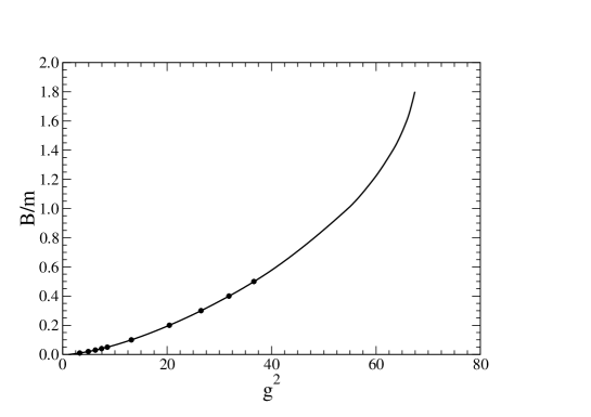
Figure 1: The binding energy $B/m$ vs $g^{2}$ for a massless vector exchange. Solid line: our calculations, with the exact analytical treatment of the end-point singularities. Full dots: $g^{2}$ from Ref. CK2010 , with a numerical treatment of the singularities. A critical value $g_{crit}$ is clearly approached for $B/m\to 2$.

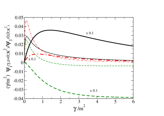
Figure 2: The light-front amplitude $\psi_{i}$ times $\gamma/m^{2}$ (cf Eq. (7)) vs $\gamma/m^{2}$ at fixed $z=0$, for the vector coupling and $B/m=0.1$ (thin lines) and $1.0$ (thick lines). Solid line: $(\gamma/m^{2})~{}\psi_{1}$. Dashed line: $(\gamma/m^{2})~{}\psi_{2}$. Dot-dashed line: $(\gamma/m^{2})~{}\psi_{4}$. Notice that $\psi_{3}=0$ for $z=0$ (see text). The lines for $B/m=1.0$ have been divide by 10.

- (1) E. E. Salpeter and H. A. Bethe, Phys. Rev. 84, 1232 (1951).
- (2) T. Frederico, G. Salmè and M. Viviani, Phys. Rev. D 85, 036009 (2012).
- (3) K. Kusaka, K. Simpson, and A. G. Williams, Phys. Rev. D 56, 5071 (1997).
- (4) V. A. Karmanov, J. Carbonell, Eur. Phys. Jou. A 27, 1 (2006).
- (5) T. Frederico, G. Salmè and M. Viviani, Phys. Rev. D 89, 016010 (2014).
- (6) C. Gutierrez, V. Gigante, T. Frederico, G. Salmè, M. Viviani and L. Tomio, Phys. Lett. B 759, 131(2016).
- (7) T. Frederico, G. Salmè and M. Viviani, Eur. Phys. J. C 75, 398 (2015).
- (8) J. Carbonell and V. A. Karmanov, Eur. Phys. J. A 46, 387 (2010).
- (9) J. Carbonell, V. A. Karmanov, Eur. Phys. Jou. A 27, 11 (2006).
- (10) S. M. Dorkin, M. Beyer, S. S. Semikh, and L. P. Kaptari, Few-Body Sys. 42 1 (2008), and private communication.
- (11) X. Ji, J.P. Ma and F. Yuan, Phys. Rev,. Lett. 90, 241601 (2003).
- (12) W. de Paula, T. Frederico, R. Pimentel, G. Salmè and M. Viviani, in preparation.
- (13) T.M. Yan , Phys. Rev. D 7, 1780 (1973).
- (14) G. Baym, Phys. Rev. 117, 886 (1960).