Error estimates on a finite volume method for diffusion problems with interface on Eulerian grids

Abstract

The finite volume methods are frequently employed in the discretization of diffusion problems with interface. In this paper, we firstly present a vertex-centered MACH-like finite volume method for solving stationary diffusion problems with strong discontinuity and multiple material cells on the Eulerian grids. This method is motivated by Frese [No. AMRC-R-874, Mission Research Corp., Albuquerque, NM, 1987]. Then, the local truncation error and global error estimates of the degenerate five-point MACH-like scheme are derived by introducing some new techniques. Especially under some assumptions, we prove that this scheme can reach the asymptotic optimal error estimate $O(h^{2}|\ln h|)$ in the maximum norm. Finally, numerical experiments verify theoretical results.

1 Introduction

Diffusion problems with interface are widely applied in multi-fluid hydrodynamic, fluid-solid coupling mechanics and many other scientific and engineering computation fields. The finite volume method (FVM), which presents local conservation and obvious advantage to handle physical models with complex characteristics very well, becomes an important discretization method for solving partial differential equations.

The finite volume methods (FVMs) based on Lagrangian and Eulerian grids are two commonly used methods for solving diffusion problems. The moving interface can be accurately described as we use the former, but the calculation is hard to execute on highly distorted grids. There are a lot of researches interested in these FVMs, e.g. [1, 2, 3, 4, 5, 6]. An advantage of the FVMs in the Eulerian frame is the reasonable shape of the computational grids, such as the uniform grids. But for the diffusion problems with strong discontinuity on the internal interface, the difficulty lies in dealing with the cells involving multiple material properties ([7]). Many researchers investigated this kind of FVMs, e.g. [8, 9, 10, 11, 12, 13, 14, 15, 16, 17, 18, 19]. Ewing constructed an immersed finite volume element method (FVEM) on a uniform triangle grid, and presented the optimal error estimate in the energy norm ([8, 9]). Shu established the superconvergence theory of a bilinear FVEM for diffusion problems with smooth coefficients on the rectangular grids ([10, 11]). Ma presented a recovery-based posterior error estimator for FVMs to solve elliptic interface problems in [12]. There also have a lot of works on the quadrilateral grids. For example, Oevermann focused on the two-dimensional (2D) and three-dimensional (3D) problems with discontinuous fluxes across the interface, and constructed a linear immersed FVEM in [13] and [14]. Ewing constructed a series of FVMs with different average methods for diffusion problems under homogeneous jump conditions, and numerical experiments were carried on to confirm the approximation order of these methods in [15]. Luce derived a kind of FVM by using a decomposition technique in [16]. Wang constructed a fourth-order compact FVM and derived some high accuracy post-processing formulas in [17]. Li proved the optimal $L^{2}$ error estimate for bilinear and biquadratic FVMs with smooth coefficients under a mesh restriction of $h^{2}$-parallelogram, respectively ([18, 19]). In addition, there are many works for the error estimates of finite element method to solve diffusion problems with smooth coefficients, for example, Nie derived the optimal $L^{2}$ error estimate of linear finite element scheme for the diffusion problem with nonlocal boundary in [20]. However, there have been few strict theoretical analyses of the global error estimation for Eulerian FVMs to solve diffusion problems with strong discontinuity and multiple material cells.

In the late 1980’s, M.H. Frese presented a finite volume method for diffusion equations in 2D magnetohydrodynamic problems on the quadrilateral grids ([21]). The corresponding software packages named MACH2 and MACH3 for 2D and 3D problems have been successfully developed, respectively, by Philips Lab/WSP, Kirtland Air Force Base ([21, 22]), and widely used in the numerical simulations of liner implosion system, plasma thrusters and so on (see, e.g. [23, 24, 25, 26, 27]). For simplicity of presentation, we denote this finite volume method as MACH FVM. However, to our knowledge, we have not found the strict error theories of it for diffusion problems with strong discontinuity and multiple material cells on the Eulerian grids, which urges us to study it.

In this paper, we present a vertex-centered MACH-like FVM on the quadrilateral grids for stationary diffusion problems with interface. In particular, for the square grids, this kind of nine-point scheme is degenerated into a five-point scheme. It is worth pointing out that many classical nine-point FVMs (see, for example, [28]) are always degenerated into a five-point stencil which looks like “+”, while the stencil of the five-point MACH-like scheme looks like “$\times$”. Therefore, this adds an extra difficulty for error estimates. The other important work of this paper is that we present the strict theoretical analysis for the five-point MACH-like scheme. It is divided into two parts. On the one hand, we discuss the local truncation error. The main difficulty results from the discontinuous coefficients of the interface. By the homogeneous jump conditions on the interface and Taylor expansions, we derive that the local truncation error of the interior nodes adjacent to the interface is $O(h)$. Furthermore, we get the local truncation error $O(h^{2})$ under the Assumption I (i.e., we use harmonic average method for the diffusion coefficients and the second derivative function with respect to the tangent direction of the exact solution is equal to zero on the interface). On the other hand, we focus on the global error estimates. Firstly, the error difference equations are decomposed into two relatively simple ones. Then, by using the discrete sine transform ([29, 30]) and combining with some analytical techniques, we convert these 2D difference equations into two kinds of one-dimensional (1D) difference equations, and the estimates of these difference equations are deduced. Hence, we demonstrate that the global error estimation of the five-point scheme is $O(h|\ln h|)$ in the maximum norm. Furthermore, under the Assumption I, we obtain the asymptotic optimal error estimate $O(h^{2}|\ln h|)$. In addition, we investigate the approximation of the five-point MACH-like scheme by several typical numerical examples. Numerical results are carried on to confirm the theoretical ones.

The paper is organized as follows. In Section 2, we describe the construction of the MACH-like finite volume method on an arbitrary quadrilateral grid, and present a five-point MACH-like scheme for special. Section 3 presents the local truncation error for the five-point scheme. Then the global error estimation in the maximum norm is derived in Section 4. After that, the accuracy of the five-point MACH-like scheme is verified numerically. In Section 6 we draw some conclusions on our works.

2 Model problem and finite volume scheme

We consider the following interface problem

$$\left\{\begin{array}[]{ll}-\nabla\cdot(\kappa\nabla u)+u=f,&\mbox{in}~{}\Omega,\\ u=0,&\mbox{on}~{}\partial\Omega,\end{array}\right.$$ (2.3)

where $\Omega\in\mathbb{R}^{2}$ is a bounded polygonal domain with boundary $\partial\Omega$, $f$ is a given function and the diffusion coefficient $\kappa$ is positive and piecewice constant on polygonal subdomains of $\Omega$ with possible large discontinuities across subdomain boundaries which is simply interface for short. Let $\kappa=\kappa_{i}>0~{}\mbox{in}~{}D_{i}$, for $i=1,2,\cdots,J$. Here $\{D_{i}\}_{i=1}^{J}$ is a partition of $\Omega$, where $D_{i}$ is an open polygonal subdomain.

Denote $\Gamma_{i,j}=\bar{D}_{i}\cap\bar{D}_{j}(i\neq j)$ and $\Gamma=\cup_{i,j=1}^{J}\Gamma_{i,j}$. We assume that

$$[u]=[\kappa\frac{\partial u}{\partial\vec{n}}]=0,~{}~{}\mbox{on}~{}\Gamma,$$ (2.4)

where $\vec{n}$ is the unit outward normal vector on $\Gamma$ and $[\zeta](\zeta=u,\kappa\frac{\partial u}{\partial\vec{n}})$ denotes the difference of the right and left limits of $\zeta$ at any point of $\Gamma$.

Let $\mathcal{Q}_{h}$ be a structured quadrilateral partition of $\Omega$, and $X=\{X_{i,j}=(x_{i},y_{j}),~{}i=0,1,\cdots,N_{x},j=0,1,\cdots,N_{y}\},$ where $N_{x},N_{y}$ are given positive integers.

Next, We derive a kind of FVM with vertex unknowns for solving (2.3) and (2.4), which is based on the method of Michael H. Frese in [21]. We denote it as MACH-like FVM for convenience.

For any given interior node $X_{i,j},i=1,2,\cdots,N_{x}-1,j=1,2,\cdots,N_{y}-1$ (see Fig. 1). We denote open area $Q_{l}(l=1,2,3,4)$ as the $l$-th quadrilateral element adjacent to $X_{i,j}$, where $O_{l},l=1,2,3,4$ are the midpoints of the grid sides $X_{i,j-1}X_{i,j},X_{i+1,j}X_{i,j},X_{i,j+1}X_{i,j}$ and $X_{i-1,j}X_{i,j}$, respectively. The quadrangle $X_{i,j}O_{l-1}A_{l}O_{l}$ is a parallelogram, where $A_{l}\in Q_{l}$. Thus, the control volume of $X_{i,j}$ is defined as the octagon area which is surrounded by $A_{l},O_{l}(l=1,2,3,4)$. We denote it briefly by $V_{i,j}$.

Fig. 1 (a) and (b) show the typical cases which have an interface in $Q_{l}(l=1,2,3,4)$ or not.

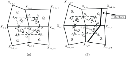
Figure 1: (a) No interface in $Q_{l}(l=1,2,3,4)$. (b) Only one interface in $Q_{2}$ and $Q_{3}$.

Integrating (2.3) over $V_{i,j}$, the equation (2.3) leads to

$$\int_{V_{i,j}}(-\nabla\cdot(\kappa\nabla u)+u)dX=\int_{V_{i,j}}fdX.$$

By the divergence theorem and the continuity condition of the flux $\kappa\frac{\partial u}{\partial\vec{n}}$, we get

$$-\int_{\partial V_{i,j}}\kappa\frac{\partial u}{\partial\vec{n}}dS+\int_{V_{i,j}}udX=\int_{V_{i,j}}fdX,$$ (2.5)

where $\partial V_{i,j}$ is the boundary of $V_{i,j}$ and $\vec{n}$ is the unit outward normal vector of $\partial V_{i,j}$.

Denote $\vec{n}_{l}$ as the unit outward normal vector on the side $O_{l-1}O_{l}$ for $l=1,2,3,4$ (see Fig. 1). Combining (2.5) and the rectangular integral formula, we can obtain

$$-\kappa_{1}^{*}(\nabla u)|_{Q_{1}}\cdot\vec{n}_{1}|O_{4}O_{1}|-\kappa_{2}^{*}(\nabla u)|_{Q_{2}}\cdot\vec{n}_{2}|O_{1}O_{2}|$$

$$-\kappa_{3}^{*}(\nabla u)|_{Q_{3}}\cdot\vec{n}_{3}|O_{2}O_{3}|-\kappa_{4}^{*}(\nabla u)|_{Q_{4}}\cdot\vec{n}_{4}|O_{3}O_{4}|+|V_{i,j}|u_{i,j}\approx\int_{V_{i,j}}fdX,$$ (2.6)

where $\kappa_{l}^{*}$ is the averaging of $\kappa$ over $Q_{l}$ and $(\nabla u)|_{Q_{l}}$ is the integral average value over $Q_{l}$.

Hence, from (2), we know that it is an urgent task to get the approximate calculation formula of $(\nabla u)|_{Q_{l}}$ for $l=1,2,3,4$.

Any open area $Q_{l}$ is shown in Fig. 2, where $X_{m}^{l}(m=1,2,3,4)$ is the vertex of $Q_{l}$, $\vec{n}_{m}^{c}(m=1,2,3,4)$ is the unit outward normal vector on the side $X_{m}^{l}X_{m+1}^{l}(m=1,2,3,4,X_{5}^{l}=X_{1}^{l})$.

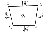
Figure 2: Illustration for $Q_{l}$.

Motivated by the finite volume method in M. H. Frese [21], we can obtain

$$(\nabla u)|_{Q_{l}} \approx \frac{1}{|Q_{l}|}[\frac{1}{2}(u(X_{1}^{l})+u(X_{2}^{l}))|X_{1}^{l}X_{2}^{l}|\vec{n}_{1}^{c}+\frac{1}{2}(u(X_{2}^{l})+u(X_{3}^{l}))|X_{2}^{l}X_{3}^{l}|\vec{n}_{2}^{c}$$ (2.7)

$$+\frac{1}{2}(u(X_{3}^{l})+u(X_{4}^{l}))|X_{3}^{l}X_{4}^{l}|\vec{n}_{3}^{c}+\frac{1}{2}(u(X_{4}^{l})+u(X_{1}^{l}))|X_{4}^{l}X_{1}^{l}|\vec{n}_{4}^{c}],$$

where $|\zeta|$ is the length or area of $\zeta$.

The option of $\kappa_{l}^{*}(l=1,2,3,4)$ is another critical element to construct the MACH-like FVM. For any given $Q_{l}(l=1,2,3,4)$, if $Q_{l}$ is a single material area (see Fig. 1(a) $Q_{k}(k=1,2,3,4)$ as an example), without loss of generality, assuming that $Q_{l}\subset D_{m}(1\leq m\leq J)$, then it follows that $\kappa_{l}^{*}=\kappa_{m}$. If $Q_{l}$ is a multiple material area (see, for example, $Q_{2},Q_{3}$ in Fig. 1(b)), then $\kappa_{l}^{*}$ must be obtained from an appropriate average method, such as arithmetic average method, harmonic average method and so on.

Substituting (2.7) into (2), and combining with the proper $\kappa_{l}^{*}(l=1,2,3,4)$, we get the MACH-like FVM of (2.3) and (2.4) at $X_{i,j}(i=1,2,\cdots,N_{x}-1,j=1,2,\cdots,N_{y}-1)$.

Remark 2.1.

The MACH-like FVM is always a compact nine-point stencil.

In particular, we consider a uniform quadrilateral grid in $\Omega=(a,b)\times(c,d)$, where

$$h_{x}=(b-a)/N_{x},~{}~{}h_{y}=(d-c)/N_{y},$$

$$(x_{i},y_{j})=(a+ih_{x},c+jh_{y}),~{}i=0,1,\cdots,N_{x},j=0,1,\cdots,N_{y}.$$

The MACH-like FVM at any interior node $X_{i,j}$ express as follows

$$a^{i,j}_{1}u_{i-1,j-1}+a^{i,j}_{2}u_{i,j-1}+a^{i,j}_{3}u_{i+1,j-1}+a^{i,j}_{4}u_{i-1,j}+a^{i,j}_{5}u_{i,j}$$

$$+a^{i,j}_{6}u_{i+1,j}+a^{i,j}_{7}u_{i-1,j+1}+a^{i,j}_{8}u_{i,j+1}+a^{i,j}_{9}u_{i+1,j+1}=h_{x}h_{y}f_{i,j},$$ (2.8)

where

$$\left\{\begin{array}[]{l}a^{i,j}_{1}=-\frac{1}{4}(\frac{h_{y}}{h_{x}}+\frac{h_{x}}{h_{y}})\kappa_{1}^{*},\\ a^{i,j}_{2}=-\frac{1}{4}(-\frac{h_{y}}{h_{x}}+\frac{h_{x}}{h_{y}})(\kappa_{1}^{*}+\kappa_{2}^{*}),\\ a^{i,j}_{3}=-\frac{1}{4}(\frac{h_{y}}{h_{x}}+\frac{h_{x}}{h_{y}})\kappa_{2}^{*},\\ a^{i,j}_{4}=-\frac{1}{4}(\frac{h_{y}}{h_{x}}-\frac{h_{x}}{h_{y}})(\kappa_{1}^{*}+\kappa_{4}^{*}),\\ a^{i,j}_{5}=\frac{1}{4}(\frac{h_{y}}{h_{x}}+\frac{h_{x}}{h_{y}})(\kappa_{1}^{*}+\kappa_{2}^{*}+\kappa_{3}^{*}+\kappa_{4}^{*})+h_{x}h_{y},\\ a^{i,j}_{6}=-\frac{1}{4}(\frac{h_{y}}{h_{x}}-\frac{h_{x}}{h_{y}})(\kappa_{2}^{*}+\kappa_{3}^{*}),\\ a^{i,j}_{7}=-\frac{1}{4}(\frac{h_{y}}{h_{x}}+\frac{h_{x}}{h_{y}})\kappa_{4}^{*},\\ a^{i,j}_{8}=-\frac{1}{4}(-\frac{h_{y}}{h_{x}}+\frac{h_{x}}{h_{y}})(\kappa_{3}^{*}+\kappa_{4}^{*}),\\ a^{i,j}_{9}=-\frac{1}{4}(\frac{h_{y}}{h_{x}}+\frac{h_{x}}{h_{y}})\kappa_{3}^{*},\\ f_{i,j}=\frac{1}{h_{x}h_{y}}\int_{V_{i,j}}fdX.\end{array}\right.$$ (2.19)

Currently, MACH scheme is successfully applied in the numerical simulation of liner implosion system, plasma thrusters and so on (see, e.g. [23, 25, 26]). However, there is few error theories about this scheme, and it is always for the local truncation error. Especially, the strict error theories for the stationary diffusion problems with multiple material cells on Eulerian grids haven’t been seen yet. In the following sections, we will establish a rigorous theoretical analysis of the MACH-like scheme, which is constructed for a simplified model of (2.3) and (2.4).

This simplified model only considers two subdomains. Suppose that $\Omega=(0,1)\times(0,1)=D_{1}\cup D_{2}\cup\Gamma$ and the diffusion coefficient

$$\kappa=\left\{\begin{array}[]{ll}\kappa^{-}\geq 1,&\mbox{in}~{}D_{1},\\ 1,&\mbox{in}~{}D_{2},\end{array}\right.$$ (2.22)

where $D_{1}=(0,\frac{1}{2})\times(0,1)$, $D_{2}=(\frac{1}{2},1)\times(0,1)$ and $\kappa^{-}$ is a positive constant.

In addition, we assume that $\mathcal{Q}_{h}$ is a square mesh of $\Omega$, where $N_{x}=N_{y}=N=2M+1(M\in\mathcal{Z}^{+})$, $h_{x}=h_{y}=h$, introduce the grid nodes and the interior nodes indicated set $S=\{(i,j),i,j=0,1,\cdots,N\}$ and $S_{0}=\{(i,j),i,j=1,2,\cdots,N-1\}$. Let the indicated set of the interior nodes which are adjacent to the interface or not be

$$S_{B}=S_{1}^{B}\cup S_{2}^{B}~{}~{}and~{}~{}S_{I}=S_{1}^{I}\cup S_{2}^{2},$$ (2.23)

respectively, where

$$S_{1}^{I}=\{(i,j),i=1,2,\cdots,M-1,j=1,2,\cdots,N-1\},$$

$$S_{2}^{I}=\{(i,j),i=M+2,M+3,\cdots,N-1,j=1,2,\cdots,N-1\},$$

$$S_{1}^{B}=\{(i,j),i=M,j=1,2,\cdots,N-1\},$$

$$S_{2}^{B}=\{(i,j),i=M+1,j=1,2,\cdots,N-1\}.$$

Denote $\kappa^{*}$ as the average value of the diffusion coefficient in the multiple material cells. From (2) and (2.19), we can obtain the five-point MACH-like scheme of the simplified model as follows

$$\left\{\begin{array}[]{ll}L_{h}u_{i,j}=h^{2}f_{i,j},&(i,j)\in S_{0},\\ u_{0,j}=u_{N,j}=u_{i,0}=u_{i,N}=0,&(i,j)\in S,\end{array}\right.$$ (2.26)

where

$$L_{h}u_{i,j}=a_{1}^{i,j}u_{i-1,j-1}+a_{2}^{i,j}u_{i+1,j-1}+a_{3}^{i,j}u_{i,j}+a_{4}^{i,j}u_{i-1,j+1}+a_{5}^{i,j}u_{i+1,j+1},~{}f_{i,j}=f(x_{i},y_{j}),$$ (2.27)

and

$$\left\{\begin{array}[]{ll}a_{1}^{i,j}=a_{2}^{i,j}=a_{4}^{i,j}=a_{5}^{i,j}=-\frac{1}{2}\kappa^{-},~{}a_{3}^{i,j}=2\kappa^{-}+h^{2},&(i,j)\in S_{1}^{I},\\ a_{1}^{i,j}=a_{4}^{i,j}=-\frac{1}{2}\kappa^{-},~{}a_{2}^{i,j}=a_{5}^{i,j}=-\frac{1}{2}\kappa^{*},~{}a_{3}^{i,j}=\kappa^{-}+\kappa^{*}+h^{2},&(i,j)\in S_{1}^{B},\\ a_{1}^{i,j}=a_{4}^{i,j}=-\frac{1}{2}\kappa^{*},~{}a_{2}^{i,j}=a_{5}^{i,j}=-\frac{1}{2},~{}a_{3}^{i,j}=\kappa^{*}+1+h^{2},&(i,j)\in S_{2}^{B},\\ a_{1}^{i,j}=a_{2}^{i,j}=a_{4}^{i,j}=a_{5}^{i,j}=-\frac{1}{2},~{}a_{3}^{i,j}=2+h^{2},&(i,j)\in S_{2}^{I}.\end{array}\right.$$

The stencil of this five-point scheme which looks like “$\times$” is shown in Fig. 3 (a). It is worth pointing out that many frequently-used nine-point FVMs, such as [28], are degenerated into a five-point stencil which looks like “+” (see Fig. 3(b)). Hence, this difference will bring some new difficulties to the following error analysis.

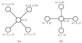
Figure 3: (a) “$\times$” type five-point stencil. (b) “+” type five-point stencil.

In the rest of this paper, we will present the rigorous error analysis and corresponding numerical experiments for the five-point MACH-like scheme (2.26).

3 Local truncation error estimation

Let

$$R_{i,j}=L_{h}u(x_{i},y_{j})-L_{h}u_{i,j}=L_{h}u(x_{i},y_{j})-h^{2}f_{i,j},~{}~{}(i,j)\in S_{0}$$ (3.1)

be the local truncation error of (2.26) at $X_{i,j}$, and denote $x_{i+\frac{1}{2}}=x_{i}+\frac{h}{2}(i=0,1,\cdots,N-1)$, $\delta_{l,m}$ as the Kronecker delta.

Define a function space via

$$W=\{w|~{}w|_{\bar{D}_{i}}\in C^{6}(\bar{D}_{i}),~{}i=1,2\}.$$

In this section, we will present the local truncation error of (2.26).

Theorem 3.1.

If $u\in W$, then the following holds.

1)

For any interior node which is non adjacent to the interface, we have

$$R_{i,j}=(\kappa^{-})^{\delta_{1,k}}C^{(4)}(x_{i},y_{j})h^{4}+O(h^{6}),~{}~{}(i,j)\in S_{k}^{I},~{}k=1,2,$$ (3.2)

where

$$C^{(4)}(x,y)=-\frac{1}{12}(\frac{\partial^{4}u}{\partial y^{4}}+\frac{\partial^{4}u}{\partial x^{4}}+6\frac{\partial^{4}u}{\partial y^{2}\partial x^{2}})(x,y).$$ (3.3)

2)

For any interior node which is adjacent to the interface, we have

$$R_{i,j}=C_{i}^{(1)}(y_{j})h+C_{i}^{(2)}(y_{j})h^{2}+C_{i}^{(3)}(y_{j})h^{3}+O(h^{4}),~{}(i,j)\in S_{B},$$ (3.4)

where

$$C_{M}^{(1)}(y)=(\kappa^{-}-\frac{\kappa^{*}}{2}-\frac{\kappa^{*}\kappa^{-}}{2})(\frac{\partial u}{\partial x})^{-}(y),~{}~{}C_{M+1}^{(1)}(y)=-C_{M}^{(1)}(y),$$ (3.5)

$$C_{M}^{(2)}(y)=\frac{\kappa^{*}}{8}[\frac{\partial^{2}u}{\partial x^{2}}](y)+\frac{1}{2}(\kappa^{-}(\frac{\partial^{2}u}{\partial y^{2}})^{-}-\kappa^{*}(\frac{\partial^{2}u}{\partial y^{2}})^{+})(y),$$ (3.6)

$$C_{M+1}^{(2)}(y)=-\frac{\kappa^{*}}{8}[\frac{\partial^{2}u}{\partial x^{2}}](y)+\frac{1}{2}((\frac{\partial^{2}u}{\partial y^{2}})^{+}-\kappa^{*}(\frac{\partial^{2}u}{\partial y^{2}})^{-})(y),$$ (3.7)

$$C_{M}^{(3)}(y)=(\frac{\kappa^{-}}{24}(\frac{\partial^{3}u}{\partial x^{3}})^{-}-\frac{\kappa^{*}}{24}\{\frac{\partial^{3}u}{\partial x^{3}}\}+\frac{1}{4}(\kappa^{-}(\frac{\partial^{3}u}{\partial y^{2}\partial x})^{-}-\kappa^{*}(\frac{\partial^{3}u}{\partial y^{2}\partial x})^{+}))(y),$$ (3.8)

$$C_{M+1}^{(3)}(y)=(-\frac{1}{24}(\frac{\partial^{3}u}{\partial x^{3}})^{+}+\frac{\kappa^{*}}{24}\{\frac{\partial^{3}u}{\partial x^{3}}\}+\frac{1}{4}(-(\frac{\partial^{3}u}{\partial y^{2}\partial x})^{+}+\kappa^{*}(\frac{\partial^{3}u}{\partial y^{2}\partial x})^{-}))(y),~{}~{}~{}~{}$$ (3.9)

and $(\zeta)^{\pm}(y):=\lim\limits_{x\rightarrow{x_{M+\frac{1}{2}}}^{\pm}}\zeta(x,y)$, $[\zeta]:=(\zeta)^{-}-(\zeta)^{+}$, $\{\zeta\}:=\frac{1}{2}((\zeta)^{-}+(\zeta)^{+})$.

Proof.

We only prove for $i=M$ and $j=1,2,\cdots,N-1$, the remainder of the argument is analogous to it.

By (2.27) and (3.1), we have

$$R_{M,j} = -\frac{1}{2}\kappa^{-}[u(x_{M-1},y_{j-1})+u(x_{M-1},y_{j+1})]-\frac{1}{2}\kappa^{*}[u(x_{M+1},y_{j-1})+u(x_{M+1},y_{j+1})]$$ (3.10)

$$+(\kappa^{-}+\kappa^{*}+h^{2})u(x_{M},y_{j})-h^{2}f(x_{M},y_{j}).$$

Substituting the Taylor series expansions of $u(x_{M\pm 1},y_{j-1})$ and $u(x_{M\pm 1},y_{j+1})$ at $(x_{M\pm 1},y_{j})$ into (3.10), we have

$$R_{M,j} = \kappa^{-}[u(x_{M},y_{j})-u(x_{M-1},y_{j})]+\kappa^{*}[u(x_{M},y_{j})-u(x_{M+1},y_{j})]$$ (3.11)

$$-\frac{1}{2}h^{2}[\kappa^{-}\frac{\partial^{2}u}{\partial y^{2}}(x_{M-1},y_{j})+\kappa^{*}\frac{\partial^{2}u}{\partial y^{2}}(x_{M+1},y_{j})]$$

$$+h^{2}u(x_{M},y_{j})-h^{2}f(x_{M},y_{j})+O(h^{4}).$$

Further, substituting the Taylor series expansions of $u(x_{M},y_{j})$, $u(x_{M\pm 1},y_{j})$, $f(x_{M},y_{j})$ and $\frac{\partial^{2}u}{\partial y^{2}}(x_{M\pm 1},y_{j})$ at $(x_{M+\frac{1}{2}},y_{j})$ into (3.11), and using $[u]|_{\Gamma}=0$, equation (2.3) and $[\kappa\frac{\partial u}{\partial\vec{n}}]|_{\Gamma}=0$, $R_{M,j}$ is rewritten as

$$R_{M,j} = h(\kappa^{-}-\frac{\kappa^{*}}{2}-\frac{\kappa^{*}\kappa^{-}}{2})(\frac{\partial u}{\partial x})^{-}(y_{j})$$ (3.12)

$$+h^{2}(\frac{\kappa^{*}}{8}[\frac{\partial^{2}u}{\partial x^{2}}]+\frac{1}{2}(\kappa^{-}(\frac{\partial^{2}u}{\partial y^{2}})^{-}-\kappa^{*}(\frac{\partial^{2}u}{\partial y^{2}})^{+}))(y_{j})$$

$$+h^{3}(\frac{\kappa^{-}}{24}(\frac{\partial^{3}u}{\partial x^{3}})^{-}-\frac{\kappa^{*}}{24}\{\frac{\partial^{3}u}{\partial x^{3}}\}+\frac{1}{4}(\kappa^{-}(\frac{\partial^{3}u}{\partial y^{2}\partial x})^{-}-\kappa^{*}(\frac{\partial^{3}u}{\partial y^{2}\partial x})^{+}))(y_{j})+O(h^{4})$$

$$=: C_{M}^{(1)}(y_{j})h+C_{M}^{(2)}(y_{j})h^{2}+C_{M}^{(3)}(y_{j})h^{3}+O(h^{4}),$$

where $C_{M}^{(1)}(y)$, $C_{M}^{(2)}(y)$ and $C_{M}^{(3)}(y)$ are defined by (3.5), (3.6) and (3.8), respectively.

This finishes the proof.

∎

For a lot of diffusion problems with interface (such as [31]), the changing of the solution along the normal direction (here for the $x$ direction) of the interfaces is far more quickly than the tangential direction (here for the $y$ direction). As a result, we suppose that

$$\lim\limits_{x\to{x_{M+\frac{1}{2}}}^{-}}\frac{\partial^{2}u}{\partial y^{2}}=\lim\limits_{x\to{x_{M+\frac{1}{2}}}^{+}}\frac{\partial^{2}u}{\partial y^{2}}=0.$$ (3.13)

Under the above assumption, we can obtain a corollary from (3.4) as follows.

Corollary 3.1.

Let $u\in W$ and suppose that $\kappa^{*}=\frac{2\kappa^{-}}{\kappa^{-}+1}$ and (3.13) are hold, then

$$R_{i,j}=\tilde{C}_{i}^{(2)}(y_{j})h^{2}+C_{i}^{(3)}(y_{j})h^{3}+O(h^{4}),~{}~{}(i,j)\in S_{B},$$ (3.14)

where

$$\tilde{C}_{M}^{(2)}(y)=\frac{\kappa^{*}}{8}[\frac{\partial^{2}u}{\partial x^{2}}](y)~{}~{}and~{}~{}\tilde{C}_{M+1}^{(2)}(y)=-\tilde{C}_{M}^{(2)}(y).$$ (3.15)

For simplicity, we denote the assumptions $\kappa^{*}=\frac{2\kappa^{-}}{\kappa^{-}+1}$ and (3.13) as Assumption I.

4 Global error estimation

In this section, we will investigate the global error estimates for the five-point MACH-like scheme.

Defined

$$\vec{e}=(e_{0,0},\cdots,e_{0,N},\cdots,e_{N,0},\cdots,e_{N,N})$$ (4.1)

as the error vector, where

$$e_{i,j}=u(x_{i},y_{j})-u_{i,j}.$$ (4.2)

Using (4.1), (4.2) and (2.26), we can obtain that $\vec{e}$ satisfies the following 2D difference equations

$$\left\{\begin{array}[]{ll}L_{h}e_{i,j}=R_{i,j},&(i,j)\in S_{0},\\ e_{i,0}=e_{i,N}=e_{0,j}=e_{N,j}=0,&(i,j)\in S,\\ \end{array}\right.$$ (4.3)

where $R_{i,j}$ for $(i,j)\in S_{0}$ are given by (3.2) and (3.4).

Let $S_{B}$ be the indicated set of the interior nodes adjacent to the interface(given by (2.23)), denote $e_{i,j}=0(\forall(i,j)\in S_{B})$ in (4.3), and we have

$$\left\{\begin{array}[]{ll}-\frac{1}{2}\kappa^{-}(e_{i-1,j-1}^{(1)}+e_{i-1,j+1}^{(1)})+(2\kappa^{-}+h^{2})e_{i,j}^{(1)}-\frac{1}{2}\kappa^{-}(e_{i+1,j-1}^{(1)}+e_{i+1,j+1}^{(1)})=R_{i,j},&(i,j)\in S_{1}^{I},\\ -\frac{1}{2}(e_{i-1,j-1}^{(1)}+e_{i-1,j+1}^{(1)})+(2+h^{2})e_{i,j}^{(1)}-\frac{1}{2}(e_{i+1,j-1}^{(1)}+e_{i+1,j+1}^{(1)})=R_{i,j},&(i,j)\in S_{2}^{I},\\ e_{i,j}^{(1)}=0,&(i,j)\in S_{B},\\ e_{0,j}^{(1)}=e_{N,j}^{(1)}=e_{i,0}^{(1)}=e_{i,N}^{(1)}=0,&(i,j)\in S.\end{array}\right.$$ (4.4)

Let $\vec{e}^{(1)}=(e_{0,0}^{(1)},\cdots,e_{0,N}^{(1)},\cdots,e_{N,0}^{(1)},\cdots,e_{N,N}^{(1)})$ be the solution vector of (4.4) and the error vector $\vec{e}$ can be decomposed as

$$\vec{e}=\vec{e}^{(1)}+\vec{e}^{(2)}.$$ (4.5)

By (4.3), (4.4) and (4.5), it is easy to check that $\vec{e}^{(2)}:=(e_{0,0}^{(2)},\cdots,e_{0,N}^{(2)},\cdots,e_{N,0}^{(2)},\cdots,e_{N,N}^{(2)})$ satisfies the following difference equations

$$\left\{\begin{array}[]{ll}-\frac{1}{2}\kappa^{-}(e_{i-1,j-1}^{(2)}+e_{i-1,j+1}^{(2)})+(2\kappa^{-}+h^{2})e_{i,j}^{(2)}-\frac{1}{2}\kappa^{-}(e_{i+1,j-1}^{(2)}+e_{i+1,j+1}^{(2)})=0,&(i,j)\in S_{1}^{I},\\ -\frac{1}{2}\kappa^{-}(e_{i-1,j-1}^{(2)}+e_{i-1,j+1}^{(2)})+(\kappa^{-}+\kappa^{*}+h^{2})e_{i,j}^{(2)}-\frac{1}{2}\kappa^{*}(e_{i+1,j-1}^{(2)}+e_{i+1,j+1}^{(2)})=\gamma_{M,j},&(i,j)\in S_{1}^{B},\\ -\frac{1}{2}\kappa^{*}(e_{i-1,j-1}^{(2)}+e_{i-1,j+1}^{(2)})+(\kappa^{*}+1+h^{2})e_{i,j}^{(2)}-\frac{1}{2}(e_{i+1,j-1}^{(2)}+e_{i+1,j+1}^{(2)})=\gamma_{M+1,j},&(i,j)\in S_{2}^{B},\\ -\frac{1}{2}(e_{i-1,j-1}^{(2)}+e_{i-1,j+1}^{(2)})+(2+h^{2})e_{i,j}^{(2)}-\frac{1}{2}(e_{i+1,j-1}^{(2)}+e_{i+1,j+1}^{(2)})=0,&(i,j)\in S_{2}^{I},\\ e_{0,j}^{(2)}=e_{N,j}^{(2)}=e_{i,0}^{(2)}=e_{i,N}^{(2)}=0,&(i,j)\in S,\end{array}\right.$$ (4.6)

where

$$\gamma_{M,j}=R_{M,j}+\frac{1}{2}\kappa^{-}(e_{M-1,j-1}^{(1)}+e_{M-1,j+1}^{(1)}),~{}~{}\gamma_{M+1,j}=R_{M+1,j}+\frac{1}{2}(e_{M+2,j-1}^{(1)}+e_{M+2,j+1}^{(1)}).$$

Then, we will employ the dimension reduction techniques (convert the 2D problems into the 1D problems) to estimate $\vec{e}^{(l)}(l=1,2)$. Therefore, for any given $i=1,2,\cdots,N-1$, $l=1,2$, introduce the discrete sine transform (see, e.g. [29]) for sequence $\{e_{i,j}^{(l)}\}_{j=1}^{N-1}$ and $\{R_{i,j}\}_{j=1}^{N-1}$ as

$$\bar{e}_{i,k}^{(l)}=\sqrt{2h}\sum\limits_{j=1}^{N-1}e_{i,j}^{(l)}\sin(j\pi y_{k}),~{}\bar{R}_{i,k}=\sqrt{2h}\sum\limits_{j=1}^{N-1}R_{i,j}\sin(j\pi y_{k}),~{}~{}k=1,2,\cdots,N-1.$$ (4.7)

Using

$$\sin(k\pi y_{j})=\sin(j\pi y_{k}),~{}~{}(k,j)\in S_{0},$$

and

$$\sum\limits_{k=1}^{N-1}\sin(k\pi y_{l})\sin(k\pi y_{m})=\frac{1}{2h}\delta_{l,m},$$

one can easily confirm

$$e_{i,j}^{(l)}=\sqrt{2h}\sum\limits_{k=1}^{N-1}\bar{e}_{i,k}^{(l)}\sin(k\pi y_{j}),~{}R_{i,j}=\sqrt{2h}\sum\limits_{k=1}^{N-1}\bar{R}_{i,k}\sin(k\pi y_{j}),~{}~{}j=1,2,\cdots,N-1,$$ (4.8)

and where the sequences $\{e_{i,j}^{(l)}\}_{j=1}^{N-1}$ and $\{R_{i,j}\}_{j=1}^{N-1}$ are called as the inverse discrete sine transform of $\{\bar{e}_{i,k}^{(l)}\}_{k=1}^{N-1}$ and $\{\bar{R}_{i,k}\}_{k=1}^{N-1}$, respectively.

Let

$$\vec{\bar{e}}_{k}^{(l)}=(\bar{e}_{0,k}^{(l)},\cdots,\bar{e}_{N,k}^{(l)}),~{}~{}k=1,2,\cdots,N-1,l=1,2,$$ (4.9)

where $\bar{e}_{i,k}^{(l)}(i=1,2,\cdots,N-1)$ is defined by (4.7), and

$$\bar{e}_{0,k}^{(l)}=\bar{e}_{N,k}^{(l)}=0.$$ (4.10)

Using (4.7) and (4.8), we can convert the estimate problems of $\vec{e}^{(l)}(l=1,2)$ into $\vec{\bar{e}}_{k}^{(l)}(k=1,2,\cdots,N-1)$.

Denote the maximum norm of any vector $\vec{\zeta}=(\zeta_{1},\cdots,\zeta_{n})$ as $\|\vec{\zeta}\|_{\infty}$, and it is calculated as $\max\limits_{i}|\zeta_{i}|$. We will present the estimation of $\|\vec{\bar{e}}_{k}^{(1)}\|_{\infty}(k=1,2,\cdots,N-1)$ firstly. It is easy to verify that $\vec{\bar{e}}_{k}^{(1)}(k=1,2,\cdots,N-1)$ satisfies the following 1D difference equations

$$\left\{\begin{array}[]{l}-\kappa^{-}\bar{e}^{(1)}_{i-1,k}\cos(k\pi h)+(2\kappa^{-}+h^{2})\bar{e}^{(1)}_{i,k}-\kappa^{-}\bar{e}^{(1)}_{i+1,k}\cos(k\pi h)=\bar{R}_{i,k},~{}i=1,2,\cdots,M-1,\\ -\bar{e}^{(1)}_{i-1,k}\cos(k\pi h)+(2+h^{2})\bar{e}^{(1)}_{i,k}-\bar{e}^{(1)}_{i+1,k}\cos(k\pi h)=\bar{R}_{i,k},~{}i=M+2,M+3,\cdots,N-1,\\ \bar{e}^{(1)}_{M,k}=\bar{e}^{(1)}_{M+1,k}=0,~{}~{}\bar{e}^{(1)}_{0,k}=\bar{e}^{(1)}_{N,k}=0.\end{array}\right.~{}~{}$$ (4.14)

As a matter of fact, using (4.7) and noting that $e_{i,j}^{(1)}=0(\forall(i,j)\in S_{B})$, we can get $\bar{e}^{(1)}_{M,k}=\bar{e}^{(1)}_{M+1,k}=0$. Hence, from (4.10), it follows that we only need to demonstrate the former $N-3$ equations of (4.14) are established.

Substituting (4.8) into the part of (4.4) where $(i,j)\in S_{1}^{I}$, we get

$$-\frac{1}{2}\kappa^{-}\sqrt{2h}\sum\limits_{k=1}^{N-1}\bar{e}_{i-1,k}^{(1)}[\sin(k\pi y_{j-1})+\sin(k\pi y_{j+1})]+(2\kappa^{-}+h^{2})\sqrt{2h}\sum\limits_{k=1}^{N-1}\bar{e}_{i,k}^{(1)}\sin(k\pi y_{j})$$

$$-\frac{1}{2}\kappa^{-}\sqrt{2h}\sum\limits_{k=1}^{N-1}\bar{e}_{i+1,k}^{(1)}[\sin(k\pi y_{j-1})+\sin(k\pi y_{j+1})]=\sqrt{2h}\sum\limits_{k=1}^{N-1}\bar{R}_{i,k}\sin(k\pi y_{j}),~{}~{}j=1,2,\cdots,N-1.~{}~{}~{}~{}~{}~{}~{}~{}$$ (4.15)

Owing to the characterization property of the discrete sine function $\sin(k\pi y_{j})(k,j=1,2,\cdots,N)$ that

$$\sin(k\pi y_{j-1})+\sin(k\pi y_{j+1})=2\sin(k\pi y_{j})\cos(k\pi h),$$

equation (4) can be further represented as

$$\sqrt{2h}\sum\limits_{k=1}^{N-1}[-\kappa^{-}\bar{e}_{i-1,k}^{(1)}\cos(k\pi h)+(2\kappa^{-}+h^{2})\bar{e}_{i,k}^{(1)}-\kappa^{-}\bar{e}_{i+1,k}^{(1)}\cos(k\pi h)-\bar{R}_{i,k}]\sin(k\pi y_{j})=0,$$

$$~{}~{}j=1,2,\cdots,N-1.$$

Therefore, we have

$$-\kappa^{-}\bar{e}_{i-1,k}^{(1)}\cos(k\pi h)+(2\kappa^{-}+h^{2})\bar{e}_{i,k}^{(1)}-\kappa^{-}\bar{e}_{i+1,k}^{(1)}\cos(k\pi h)-\bar{R}_{i,k}=0,~{}~{}k=1,2,\cdots,N-1.~{}~{}~{}~{}~{}~{}~{}~{}$$

Namely, the former $M-1$ equations of (4.14) are established.

The rest of the proof is similar to before. The proof is completed.

In order to estimate $\|\vec{\bar{e}}_{k}^{(1)}\|_{\infty}(k=1,2,\cdots,N-1)$ by using the difference equations (4.14), we need to introduce several lemmas as follows.

Lemma 4.1.

Let $\varphi_{j}:=\varphi(y_{j})(j=1,2,\cdots,N-1)$, and assume that $\varphi(y)\in C^{2}([0,1])$, then

$$|\sum\limits_{j=1}^{N-1}\varphi_{j}\sin(j\pi y_{k})| \lesssim \frac{\|\varphi\|_{2,\infty}}{\sin\frac{k\pi h}{2}}.$$ (4.16)

Proof.

Since

$$\sum\limits_{j=2}^{N-2}(\varphi_{j-1}+\varphi_{j+1})\sin(j\pi y_{k}) = \sum\limits_{j=1}^{N-3}\varphi_{j}\sin((j+1)\pi y_{k})+\sum\limits_{j=3}^{N-1}\varphi_{j}\sin((j-1)\pi y_{k})$$

$$= 2\cos(\pi y_{k})\sum\limits_{j=1}^{N-1}\varphi_{j}\sin(j\pi y_{k})-\sin(\pi y_{k})((-1)^{k-1}\varphi_{N-2}-\varphi_{2}),$$

we have

$$(\cos(\pi y_{k})-1)\sum\limits_{j=1}^{N-1}\varphi_{j}\sin(j\pi y_{k}) = \sum\limits_{j=2}^{N-2}(\frac{\varphi_{j-1}+\varphi_{j+1}}{2}-\varphi_{j})\sin(j\pi y_{k})$$

$$+\sin(\pi y_{k})((-1)^{k-1}(\frac{1}{2}\varphi_{N-2}-\varphi_{N-1})+(\frac{1}{2}\varphi_{2}-\varphi_{1})).$$

As this result, and noting that $\cos(\pi y_{k})-1=-2\sin^{2}\frac{k\pi h}{2}\neq 0(k=1,2,\cdots,N-1)$, one we can obtain

$$\sum\limits_{j=1}^{N-1}\varphi_{j}\sin(j\pi y_{k}) = -\frac{1}{2\sin^{2}\frac{k\pi h}{2}}\sum\limits_{j=2}^{N-2}(\frac{\varphi_{j-1}+\varphi_{j+1}}{2}-\varphi_{j})\sin(j\pi y_{k})$$ (4.17)

$$+\frac{\cos\frac{k\pi h}{2}}{\sin\frac{k\pi h}{2}}(-(\frac{1}{2}\varphi_{2}-\varphi_{1})+(-1)^{k}(\frac{1}{2}\varphi_{N-2}-\varphi_{N-1})).$$

Using

$$\sin x\geq\frac{2}{\pi}x,~{}\forall x\in(0,\frac{\pi}{2}),$$ (4.18)

we get

$$\sin\frac{k\pi h}{2}\geq kh>0.$$ (4.19)

From (4.17) and (4.19), it follows

$$|\sum\limits_{j=1}^{N-1}\varphi_{j}\sin(j\pi y_{k})| \lesssim \frac{h^{-1}}{k\sin\frac{k\pi h}{2}}\sum\limits_{j=2}^{N-2}|\frac{\varphi_{j-1}+\varphi_{j+1}}{2}-\varphi_{j}|$$ (4.20)

$$+\frac{1}{\sin\frac{k\pi h}{2}}(|\varphi_{2}|+|\varphi_{1}|+|\varphi_{N-2}|+|\varphi_{N-1}|)$$

$$\lesssim \frac{h^{-1}}{k\sin\frac{k\pi h}{2}}\sum\limits_{j=2}^{N-2}|\frac{\varphi_{j-1}+\varphi_{j+1}}{2}-\varphi_{j}|+\frac{\|\varphi\|_{\infty}}{\sin\frac{k\pi h}{2}}.$$

Noting that $\varphi(y)\in C^{2}([0,1])$ and by the Taylor series expansions of $\varphi_{j\pm 1}$ at $y=y_{j}$, we have

$$|\frac{\varphi_{j-1}+\varphi_{j+1}}{2}-\varphi_{j}|\lesssim h^{2}\|\varphi^{\prime\prime}\|_{\infty},~{}~{}j=2,3,\cdots,N-2.$$ (4.21)

Using (4.20), (4.21) and paying attention to $N=h^{-1}$, (4.16) holds. ∎

Set the integer $K>3$, $\beta\in\mathbb{R}$, a $K\times K$ square matrix is defined by

$$T=\left(\begin{array}[]{cccc}\beta&-1&&\\ -1&\beta&-1&\\ &\ddots&\ddots&\ddots\\ &&-1&\beta\\ \end{array}\right).$$ (4.26)

For any given real number $\lambda$, let

$$Z_{j}(\lambda) = \lambda^{j}-\lambda^{-j},~{}j=0,1,2,\cdots.$$ (4.27)

If $|\lambda|>1$, paying attention to $Z_{0}(\lambda)=0$ and $|Z_{j}(\lambda)|=|\lambda|^{j}-|\lambda|^{-j}$ , we have

$$\frac{|Z_{j}(\lambda)|}{|Z_{i}(\lambda)|}<1,~{}~{}1\leq j<i.$$ (4.28)

The following lemma presents the estimation of the elements of $T^{-1}$, where $T^{-1}$ is the inverse of $T$.

Lemma 4.2.

If $|\beta|>2$, $T$ is defined by (4.26) and $T^{-1}:=(\tilde{t}_{i,j})_{K\times K}$, then

$$|\tilde{t}_{i,i}|=\max\limits_{j}|\tilde{t}_{i,j}|, i=1,2,\cdots,K,$$ (4.29)

and

$$\tilde{t}_{K,K}<1.$$ (4.30)

Proof.

Since $TT^{-1}=I$, for any given $i=1,2,\cdots,K$, it follows

$$\left\{\begin{array}[]{ll}\beta\tilde{t}_{i,1}-\tilde{t}_{i,2}=\delta_{i,1},&\\ -\tilde{t}_{i,j-1}+\beta\tilde{t}_{i,j}-\tilde{t}_{i,j+1}=\delta_{i,j},&j=2,3,\cdots,K-1,\\ -\tilde{t}_{i,K-1}+\beta\tilde{t}_{i,K}=\delta_{i,K}.&\end{array}\right.$$ (4.34)

Noticing that the characteristic equation of (4.34) is

$$\lambda^{2}-\beta\lambda+1=0.$$ (4.35)

Using $|\beta|>2$, we get the characteristic root of equation (4.35) with its absolute value greater than 1 as follows

$$\lambda_{\beta}=sgn(\beta)\left(\frac{|\beta|}{2}+\sqrt{(\frac{\beta}{2})^{2}-1}\right),$$ (4.36)

where $sgn(\cdot)$ is the sign function.

By (4.36), we can easily confirm that the component solution of difference equations (4.34) is

$$\tilde{t}_{i,j}=\left\{\begin{array}[]{ll}\frac{Z_{K-i+1}(\lambda_{\beta})Z_{j}(\lambda_{\beta})}{Z_{K+1}(\lambda_{\beta})Z_{1}(\lambda_{\beta})},&\mbox{if}~{}j=1,2,\cdots,i,\\ \frac{Z_{i}(\lambda_{\beta})Z_{K-j+1}(\lambda_{\beta})}{Z_{K+1}(\lambda_{\beta})Z_{1}(\lambda_{\beta})},&\mbox{if}~{}j=i+1,i+2,\cdots,K.\end{array}\right.$$ (4.39)

Hence, using (4.39), we get

$$\frac{|\tilde{t}_{i,j}|}{|\tilde{t}_{i,i}|}=\left\{\begin{array}[]{ll}\frac{|Z_{j}(\lambda_{\beta})|}{|Z_{i}(\lambda_{\beta})|},&\mbox{if}~{}j=1,2,\cdots,i,\\ \frac{|Z_{K-j+1}(\lambda_{\beta})|}{|Z_{K-i+1}(\lambda_{\beta})|},&\mbox{if}~{}j=i+1,i+2,\cdots,K.\end{array}\right.$$ (4.42)

Noticing that $|\lambda_{\beta}|>1$, from (4.28) and (4.42), we have (4.29).

By using (4.27), (4.39) and (4.36), we have

$$\beta\tilde{t}_{i,i}=\beta sgn(\lambda_{\beta})\frac{|Z_{K-i+1}(\lambda_{\beta})||Z_{i}(\lambda_{\beta})|}{|Z_{K+1}(\lambda_{\beta})||Z_{1}(\lambda_{\beta})|}>0.$$ (4.43)

From (4.34), (4.29), (4.43) and $|\beta|>2$, then we have

$$1=-\tilde{t}_{K,K-1}+\beta\tilde{t}_{K,K}\geq-|\tilde{t}_{K,K}|+\beta\tilde{t}_{K,K}\geq(|\beta|-1)|\tilde{t}_{K,K}|>|\tilde{t}_{K,K}|.$$

That is to say (4.30) holds.

∎

For any given vector $\vec{\alpha}=(\alpha_{1},\cdots,\alpha_{K})^{T}\in\mathbb{R}^{K}$, we consider

$$T\vec{s}=\vec{\alpha},$$ (4.44)

where $T$ is defined by (4.26) and $\vec{s}=(s_{1},\cdots,s_{K})^{T}$.

Corollary 4.1.

Under the assumptions as Lemma 4.2, we have the last component of the solution vector of (4.44) satisfies

$$|s_{K}|<K\|\vec{\alpha}\|_{\infty}.$$ (4.45)

Proof.

Using $\vec{s}=T^{-1}\vec{\alpha}$, (4.29) and (4.30), we have

$$|s_{K}|=|\sum\limits_{j=1}^{K}\tilde{t}_{K,j}\alpha_{j}|\leq\|\vec{\alpha}\|_{\infty}\sum\limits_{j=1}^{K}|\tilde{t}_{K,j}|\leq\|\vec{\alpha}\|_{\infty}K|\tilde{t}_{K,K}|<\|\vec{\alpha}\|_{\infty}K,$$

which completes the proof of (4.45). ∎

Using the above lemmas and corollary, we can get the estimation of $\|\vec{\bar{e}}_{k}^{(1)}\|_{\infty}(k=1,2,\cdots,N-1)$.

Theorem 4.1.

If $u\in W$, then

$$\|\vec{\bar{e}}_{k}^{(1)}\|_{\infty}\lesssim\frac{h^{\frac{3}{2}}}{k},~{}~{}k=1,2,\cdots,N-1,$$ (4.46)

and

$$|\bar{e}^{(1)}_{M-1,k}|\lesssim\frac{h^{\frac{7}{2}}}{\sin\frac{k\pi h}{2}|\cos(k\pi h)|},~{}~{}|\bar{e}^{(1)}_{M+2,k}|\lesssim\frac{h^{\frac{7}{2}}}{\sin\frac{k\pi h}{2}|\cos(k\pi h)|}.$$ (4.47)

Proof.

Noticing that the inequation of (4.46) holds if and only if

$$\max\limits_{0\leq i\leq M}|\bar{e}_{i,k}^{(1)}|\lesssim\frac{h^{\frac{3}{2}}}{k}~{}\mbox{and}~{}\max\limits_{M+1\leq i\leq N}|\bar{e}_{i,k}^{(1)}|\lesssim\frac{h^{\frac{3}{2}}}{k}.$$ (4.48)

Now we turn to prove the first inequation of (4.47) and (4.48), respectively, the second inequation of (4.47) and (4.48) can be proved similarly.

For any given $k=1,2,\cdots,N-1$ and using (4.14), one can obtain that $\{\bar{e}_{i,k}^{(1)}\}_{i=0}^{M}$ satisfies the following difference equations

$$\left\{\begin{array}[]{ll}\bar{L}_{h}\bar{e}^{(1)}_{i,k}=\bar{R}_{i,k},&i=1,2,\cdots,M-1,\\ \bar{e}^{(1)}_{0,k}=\bar{e}^{(1)}_{M,k}=0,\end{array}\right.$$ (4.51)

where $\bar{L}_{h}\bar{e}^{(1)}_{i,k}:=-\kappa^{-}\bar{e}^{(1)}_{i-1,k}\cos(k\pi h)+(2\kappa^{-}+h^{2})\bar{e}^{(1)}_{i,k}-\kappa^{-}\bar{e}^{(1)}_{i+1,k}\cos(k\pi h)$.

Comparing (4.51) with (4.44), and using Corollary 4.1, where $s_{i}:=\kappa^{-}\bar{e}^{(1)}_{i,k}\cos(k\pi h)$, $|\beta|:=|\frac{2\kappa^{-}+h^{2}}{\kappa^{-}\cos(k\pi h)}|>2$, $\alpha_{i}:=\bar{R}_{i,k}$ and $K:=M-1$, we get

$$|\kappa^{-}\bar{e}_{M-1,k}\cos(k\pi h)|=|s_{K}|<K\|\vec{\alpha}\|_{\infty}<M\max\limits_{1\leq i\leq M-1}|\bar{R}_{i,k}|.$$

Hence, by using $\kappa^{-}\geq 1$ (see (2.22)), we have

$$|\bar{e}_{M-1,k}|<\frac{M\max\limits_{1\leq i\leq M-1}|\bar{R}_{i,k}|}{\kappa^{-}|\cos(k\pi h)|}.$$ (4.52)

Noticing that $u\in W$, from (4.7) and (3.2), we have

$$|\bar{R}_{i,k}|\lesssim h^{\frac{9}{2}}|\sum\limits_{j=1}^{N-1}C^{(4)}(x_{i},y_{j})\sin(j\pi y_{k})|+h^{\frac{11}{2}},~{}i=1,2,\cdots,M-1.$$ (4.53)

Using (3.3) and Lemma 4.1, we get

$$|\sum\limits_{j=1}^{N-1}C^{(4)}(x_{i},y_{j})\sin(j\pi y_{k})|\lesssim\frac{1}{\sin\frac{k\pi h}{2}},~{}~{}i=1,2,\cdots,M-1.$$

Substituting this into (4.53), we can obtain

$$|\bar{R}_{i,k}|\lesssim\frac{h^{\frac{9}{2}}}{\sin\frac{k\pi h}{2}},~{}i=1,2,\cdots,M-1.$$ (4.54)

Using (4.52) and (4.54), we have the first inequation of (4.47) is established.

Let

$$E_{j}=(1+x_{j})h^{-2}\max\limits_{1\leq i\leq M-1}|\bar{R}_{i,k}|,~{}~{}j=0,1,\cdots,M.$$ (4.55)

Noticing that $\bar{L}_{h}(1+x_{j})>h^{2}$, together with (4.55) and (4.51), we obtain

$$\bar{L}_{h}E_{j}>\max\limits_{1\leq i\leq M-1}|\bar{R}_{i,k}|\geq|\bar{L}_{h}\bar{e}_{j,k}^{(1)}|,~{}~{}j=1,2,\cdots,M-1.$$ (4.56)

Thus, using (4.56), and paying attention to $E_{0}>|\bar{e}^{(1)}_{0,k}|,E_{M}>|\bar{e}^{(1)}_{M,k}|$, by comparison theorem, we have

$$|\bar{e}^{(1)}_{j,k}|<E_{j}\lesssim h^{-2}\max\limits_{1\leq i\leq M-1}|\bar{R}_{i,k}|,~{}~{}j=1,2,\cdots,M-1.$$ (4.57)

Hence, from (4.57), (4.54) and (4.19), the first inequation of (4.48) holds.

The proof is completed.

∎

Then, we will estimate $\|\vec{\bar{e}}_{k}^{(2)}\|_{\infty}(k=1,2,\cdots,N-1)$.

Using (4.6), (4.7) and (4.8), similar to the derivation process of (4.14), we can obtain the 1D difference equations that $\vec{\bar{e}}_{k}^{(2)}(k=1,2,\cdots,N-1)$ satisfies as follows

$$\left\{\begin{array}[]{l}-\kappa^{-}\bar{e}^{(2)}_{i-1,k}\cos(k\pi h)+(2\kappa^{-}+h^{2})\bar{e}^{(2)}_{i,k}-\kappa^{-}\bar{e}^{(2)}_{i+1,k}\cos(k\pi h)=0,~{}~{}i=1,2,\cdots,M-1,\\ -\bar{e}^{(2)}_{i-1,k}\cos(k\pi h)+(2+h^{2})\bar{e}^{(2)}_{i,k}-\bar{e}^{(2)}_{i+1,k}\cos(k\pi h)=0,~{}~{}i=M+2,M+3,\cdots,N-1,\\ -\kappa^{-}\bar{e}^{(2)}_{M-1,k}\cos(k\pi h)+(\kappa^{-}+\kappa^{*}+h^{2})\bar{e}^{(2)}_{M,k}-\kappa^{*}\bar{e}_{M+1,k}^{(2)}\cos(k\pi h)=\bar{\gamma}_{M,k},\\ -\kappa^{*}\bar{e}^{(2)}_{M,k}\cos(k\pi h)+(\kappa^{*}+1+h^{2})\bar{e}^{(2)}_{M+1,k}-\bar{e}^{(2)}_{M+2,k}\cos(k\pi h)=\bar{\gamma}_{M+1,k},\\ \bar{e}^{(2)}_{0,k}=\bar{e}^{(2)}_{N,k}=0,\end{array}\right.$$ (4.63)

where

$$\bar{\gamma}_{M,k}=\bar{R}_{M,k}+\kappa^{-}\bar{e}^{(1)}_{M-1,k}\cos(k\pi h),~{}~{}\bar{\gamma}_{M+1,k}=\bar{R}_{M+1,k}+\bar{e}^{(1)}_{M+2,k}\cos(k\pi h).$$ (4.64)

Lemma 4.3.

If function $Z_{j}$ is defined by (4.27), then, for any given $k=1,2,\cdots,N-1$, $\vec{\bar{e}}_{k}^{(2)}$ satisfies

$$\bar{e}^{(2)}_{M,k}=\frac{\bar{\gamma}_{M,k}\delta_{k}(1)+\bar{\gamma}_{M+1,k}\kappa^{*}}{(\delta_{k}(\kappa^{-})\delta_{k}(1)-(\kappa^{*})^{2})\cos(k\pi h)},~{}~{}\bar{e}^{(2)}_{M+1,k}=\frac{\bar{\gamma}_{M+1,k}+\kappa^{*}\cos(k\pi h)\bar{e}^{(2)}_{M,k}}{\delta_{k}(1)\cos(k\pi h)},$$ (4.65)

and

$$\bar{e}^{(2)}_{i,k}=\left\{\begin{array}[]{ll}\frac{Z_{i}(\lambda_{k}(\kappa^{-}))}{Z_{M}(\lambda_{k}(\kappa^{-}))}\bar{e}^{(2)}_{M,k},&\mbox{if}~{}i=0,1,\cdots,M-1,\\ \frac{Z_{N-i}(\lambda_{k}(1))}{Z_{M}(\lambda_{k}(1))}\bar{e}^{(2)}_{M+1,k},&\mbox{if}~{}i=M+2,M+3,\cdots,N,\end{array}\right.$$ (4.66)

where ($\omega=\kappa^{-},1$)

$$\lambda_{k}(\omega)=sgn(\cos(k\pi h))\left(\frac{1}{|\cos(k\pi h)|}(1+\frac{h^{2}}{2\omega})+\sqrt{\frac{1}{\cos^{2}(k\pi h)}(1+\frac{h^{2}}{2\omega})^{2}-1}\right),$$ (4.67)

$$\delta_{k}(\omega)=\Theta_{k}(\omega)+\frac{\kappa^{*}+h^{2}}{\cos(k\pi h)},~{}~{}\Theta_{k}(\omega)=\omega(\frac{1}{\cos(k\pi h)}-\frac{Z_{M-1}(\lambda_{k}(\omega))}{Z_{M}(\lambda_{k}(\omega))}).$$ (4.68)

Proof.

Using the former $2M-2$ equations of (4.63), and $\bar{e}^{(2)}_{0,k}=\bar{e}^{(2)}_{N,k}=0$, we have

$$\left\{\begin{array}[]{l}(2\kappa^{-}+h^{2})\bar{e}^{(2)}_{1,k}-\kappa^{-}\bar{e}^{(2)}_{2,k}\cos(k\pi h)=0,\\ -\kappa^{-}\bar{e}^{(2)}_{i-1,k}\cos(k\pi h)+(2\kappa^{-}+h^{2})\bar{e}^{(2)}_{i,k}-\kappa^{-}\bar{e}^{(2)}_{i+1,k}\cos(k\pi h)=0,~{}i=2,3,\cdots,M-2,{}{}{}{}\\ -\kappa^{-}\bar{e}^{(2)}_{M-2,k}\cos(k\pi h)+(2\kappa^{-}+h^{2})\bar{e}^{(2)}_{M-1,k}=\kappa^{-}\bar{e}^{(2)}_{M,k}\cos(k\pi h),\end{array}\right.$$ (4.72)

and

$$\left\{\begin{array}[]{l}(2+h^{2})\bar{e}^{(2)}_{M+2,k}-\bar{e}^{(2)}_{M+3,k}\cos(k\pi h)=\bar{e}^{(2)}_{M+1,k}\cos(k\pi h),\\ -\bar{e}^{(2)}_{i-1,k}\cos(k\pi h)+(2+h^{2})\bar{e}^{(2)}_{i,k}-\bar{e}^{(2)}_{i+1,k}\cos(k\pi h)=0,~{}~{}i=M+3,M+4,\cdots,N-2,\\ -\bar{e}^{(2)}_{N-2,k}\cos(k\pi h)+(2+h^{2})\bar{e}^{(2)}_{N-1,k}=0.\end{array}\right.$$ (4.76)

By using (4.72), similar to the derivation process of (4.39)($\beta:=\frac{2\kappa^{-}+h^{2}}{\kappa^{-}\cos(k\pi h)}$, $\lambda_{\beta}:=\lambda_{k}(\kappa^{-})$), we have

$$\bar{e}^{(2)}_{i,k}=\frac{Z_{i}(\lambda_{k}(\kappa^{-}))}{Z_{M}(\lambda_{k}(\kappa^{-}))}\bar{e}^{(2)}_{M,k},~{}~{}i=0,1,\cdots,M-1.$$

Similarly, by (4.76), we have

$$\bar{e}^{(2)}_{i,k}=\frac{Z_{N-i}(\lambda_{k}(1))}{Z_{M}(\lambda_{k}(1))}\bar{e}^{(2)}_{M+1,k},~{}~{}i=M+2,M+3,\cdots,N,$$

which completes the proof of (4.66).

Then using the $2M-1$-th and $2M$-th equation of (4.66), one can obtain

$$\left\{\begin{array}[]{ll}\delta_{k}(\kappa^{-})\cos(k\pi h)\bar{e}^{(2)}_{M,k}-\kappa^{*}\cos(k\pi h)\bar{e}_{M+1,k}^{(2)}=\bar{\gamma}_{M,k},\\ -\kappa^{*}\cos(k\pi h)\bar{e}^{(2)}_{M,k}+\delta_{k}(1)\cos(k\pi h)\bar{e}^{(2)}_{M+1,k}=\bar{\gamma}_{M+1,k},\end{array}\right.$$

where $\delta_{k}(\omega)$ is defined by (4.68).

Solving the above equations, we deduce that $\bar{e}^{(2)}_{M,k}$ and $\bar{e}^{(2)}_{M+1,k}$ satisfy (4.65). ∎

In order to estimate $\vec{\bar{e}}_{k}^{(2)}$ by (4.65) and (4.66), we introduce the following two lemmas.

Lemma 4.4.

$$\delta_{k}(\kappa^{-})\geq\delta_{k}(1)>\kappa^{*}+kh, ~{}~{}\mbox{if}~{}k=1,2,\cdots,M,$$ (4.78)

$$-\delta_{k}(\kappa^{-})\geq-\delta_{k}(1)>\kappa^{*}+(N-k)h, ~{}~{}\mbox{if}~{}k=M+1,M+2,\cdots,N-1.$$ (4.79)

Proof.

We only give the proof of (4.78), and (4.79) can be proved similarly.

First of all, we have to prove

$$\delta_{k}(\kappa^{-})\geq\delta_{k}(1),~{}~{}k=1,2,\cdots,M.$$ (4.80)

In fact, from (4.68), we know that if we can prove

$$\Theta_{k}(\kappa^{-})\geq\Theta_{k}(1),~{}~{}k=1,2,\cdots,M,$$ (4.81)

then (4.80) follows immediately.

Using (4.67) and

$$0<\cos(k\pi h)<1,~{}~{}k=1,2,\cdots,M,$$ (4.82)

we have

$$\frac{\omega}{\cos(k\pi h)}=\omega\lambda_{k}(\omega)-\frac{h^{2}}{2\cos(k\pi h)}-\eta(\omega),$$ (4.83)

where $\eta(\omega)=\sqrt{(\frac{2\omega+h^{2}}{2\cos(k\pi h)})^{2}-\omega^{2}}$.

Hence, from (4.68) and (4.83), we have

$$\Theta_{k}(\omega)=\omega(\lambda_{k}(\omega)-\frac{Z_{M-1}(\lambda_{k}(\omega))}{Z_{M}(\lambda_{k}(\omega))})-\frac{h^{2}}{2\cos(k\pi h)}-\eta(\omega).$$ (4.84)

By (4.27) and (4.67), it follows that

$$w(\lambda_{k}(\omega)-\frac{Z_{M-1}(\lambda_{k}(\omega))}{Z_{M}(\lambda_{k}(\omega))})=w\frac{\lambda_{k}(\omega)-(\lambda_{k}(\omega))^{-1}}{1-(\lambda_{k}(\omega))^{-2M}}=\frac{2\eta(\omega)}{1-(\lambda_{k}(\omega))^{-2M}}.$$ (4.85)

Thus, substituting (4.85) into (4.84), we have

$$\Theta_{k}(\omega)=(\frac{2}{1-(\lambda_{k}(\omega))^{-2M}}-1)\eta(\omega)-\frac{h^{2}}{2\cos(k\pi h)}.$$ (4.86)

From (4.67) and $\kappa^{-}\geq 1$, one can obtain

$$\lambda_{k}(1)\geq\lambda_{k}(\kappa^{-})>1,~{}~{}k=1,2,\cdots,M.$$ (4.87)

Therefore, by using (4.86), (4.87), the characteristic that $\eta(\omega)$ is increasing monotone with $w>0$ and $\kappa^{-}\geq 1$, we have (4.81) established.

Then, we want to illustrate

$$\delta_{k}(1)-\kappa^{*}>kh,~{}~{}k=1,2,\cdots,M.$$ (4.88)

Using (4.68) and (4.82), we get

$$\delta_{k}(1)-\kappa^{*}>\Theta_{k}(1).$$ (4.89)

From (4.86) and $\lambda_{k}(1)>1$, we have

$$\Theta_{k}(1)>\eta(1)-\frac{h^{2}}{2\cos(k\pi h)}.$$ (4.90)

For $k=1,2,\cdots,M$ and using (4.18), it follows

$$\frac{1}{\cos^{2}(k\pi h)}>1+4k^{2}h^{2}~{}~{}and~{}~{}\frac{1}{\cos(k\pi h)}\leq h^{-1},~{}~{}k=1,2,\cdots,M.$$

From this, one can obtain

$$\eta(1)\geq\sqrt{(1+\frac{h^{2}}{2})^{2}(1+4k^{2}h^{2})-1}>2kh~{}~{}and~{}~{}\frac{h^{2}}{2\cos(k\pi h)} \leq \frac{h}{2}.$$ (4.91)

Combining (4.89), (4.90) and (4.91), we get (4.88).

In conclusion, using (4.80) and (4.88), we finish the proof of (4.78).

∎

By using Lemma 4.4, it is obvious that

$$|\delta_{k}(\kappa^{-})|\geq|\delta_{k}(1)|>\kappa^{*}.$$ (4.92)

Lemma 4.5.

For any given $k=1,2,\cdots,N-1$, if $u\in W$, then

$$|\bar{\gamma}_{M+1,k}|\lesssim\frac{h^{\frac{3}{2}}}{\sin\frac{k\pi h}{2}},$$ (4.93)

$$|\bar{\gamma}_{M,k}\delta_{k}(1)+\bar{\gamma}_{M+1,k}\kappa^{*}|\lesssim\frac{h^{\frac{3}{2}}}{\sin\frac{k\pi h}{2}}(|\delta_{k}(1)-\kappa^{*}|+h|\delta_{k}(1)|).$$ (4.94)

Further, if the Assumption I is established, then

$$|\bar{\gamma}_{M+1,k}|\lesssim\frac{h^{\frac{5}{2}}}{\sin\frac{k\pi h}{2}},$$ (4.95)

$$|\bar{\gamma}_{M,k}\delta_{k}(1)+\bar{\gamma}_{M+1,k}\kappa^{*}|\lesssim\frac{h^{\frac{5}{2}}}{\sin\frac{k\pi h}{2}}(|\delta_{k}(1)-\kappa^{*}|+h|\delta_{k}(1)|).$$ (4.96)

Proof.

Using (4.7), (3.4), (3.5) and Lemma 4.1, similar to the proof of (4.54) shows that

$$|\bar{R}_{M+1,k}|\lesssim\frac{h^{\frac{3}{2}}}{\sin\frac{k\pi h}{2}},~{}~{}k=1,2,\cdots,N-1.$$ (4.97)

Similarly, if the Assumption I is established, by using (4.7), (3.14), (3.15) and Lemma 4.1, we have

$$|\bar{R}_{M+1,k}|\lesssim\frac{h^{\frac{5}{2}}}{\sin\frac{k\pi h}{2}},~{}~{}k=1,2,\cdots,N-1.$$ (4.98)

Therefore, from (4.64), (4.47) and (4.97), we get (4.93). Similarly, using (4.98), we get (4.95).

The rest is to show that (4.94) and (4.96) are established.

Using (4.64) and (4.7), it follows

$$|\bar{\gamma}_{M,k}\delta_{k}(1)+\bar{\gamma}_{M+1,k}\kappa^{*}|$$ (4.99)

$$\leq |\bar{R}_{M,k}\delta_{k}(1)+\bar{R}_{M+1,k}\kappa^{*}|+\kappa^{-}|\bar{e}_{M-1,k}^{(1)}\cos(k\pi h)||\delta_{k}(1)|+|\bar{e}_{M+2,k}^{(1)}\cos(k\pi h)|\kappa^{*}$$

$$= \beta_{1}+\kappa^{-}|\bar{e}_{M-1,k}^{(1)}\cos(k\pi h)||\delta_{k}(1)|+|\bar{e}_{M+2,k}^{(1)}\cos(k\pi h)|\kappa^{*},$$

where

$$\beta_{1}=\sqrt{2h}|\sum\limits_{j=1}^{N-1}(R_{M,j}\delta_{k}(1)+R_{M+1,j}\kappa^{*})\sin(j\pi y_{k})|.$$ (4.100)

By (4.47) and Lemma 4.4, we have

$$\kappa^{-}|\bar{e}_{M-1,k}^{(1)}\cos(k\pi h)||\delta_{k}(1)|+|\bar{e}_{M+2,k}^{(1)}\cos(k\pi h)|\kappa^{*}\lesssim|\delta_{k}(1)|\frac{h^{\frac{7}{2}}}{\sin\frac{k\pi h}{2}}.$$ (4.101)

Hence, substituting (4.101) into (4.99), we can obtain

$$|\bar{\gamma}_{M,k}\delta_{k}(1)+\bar{\gamma}_{M+1,k}\kappa^{*}|\lesssim\beta_{1}+|\delta_{k}(1)|\frac{h^{\frac{7}{2}}}{\sin\frac{k\pi h}{2}}.$$ (4.102)

Using (4.100), (3.4) and (3.5), and noticing that (4.92), we can obtain

$$\beta_{1} \lesssim h^{\frac{3}{2}}|\delta_{k}(1)-\kappa^{*}||\sum\limits_{j=1}^{N-1}C_{M}^{(1)}(y_{j})\sin(j\pi y_{k})|$$ (4.103)

$$+h^{\frac{5}{2}}|\sum\limits_{j=1}^{N-1}(C_{M}^{(2)}(y_{j})\delta_{k}(1)+C_{M+1}^{(2)}(y_{j})\kappa^{*})\sin(j\pi y_{k})|+h^{\frac{5}{2}}|\delta_{k}(1)|$$

$$\leq h^{\frac{3}{2}}|\delta_{k}(1)-\kappa^{*}||\sum\limits_{j=1}^{N-1}C_{M}^{(1)}(y_{j})\sin(j\pi y_{k})|$$

$$+h^{\frac{5}{2}}|\delta_{k}(1)|(|\sum\limits_{j=1}^{N-1}C_{M}^{(2)}(y_{j})\sin(j\pi y_{k})|+|\sum\limits_{j=1}^{N-1}C_{M+1}^{(2)}(y_{j})\sin(j\pi y_{k})|+h^{\frac{5}{2}}|\delta_{k}(1)|.~{}~{}$$

Further, if Assumption I holds, by similar derivation of (4.103), using (4.100), (3.14), (3.15), and noticing that (4.92) holds, we have

$$\beta_{1} \lesssim h^{\frac{5}{2}}|\delta_{k}(1)-\kappa^{*}||\sum\limits_{j=1}^{N-1}\tilde{C}_{M}^{(2)}(y_{j})\sin(j\pi y_{k})|$$ (4.104)

$$+h^{\frac{7}{2}}|\delta_{k}(1)|(|\sum\limits_{j=1}^{N-1}C_{M}^{(3)}(y_{j})\sin(j\pi y_{k})|+|\sum\limits_{j=1}^{N-1}C_{M+1}^{(3)}(y_{j})\sin(j\pi y_{k})|)+h^{\frac{7}{2}}|\delta_{k}(1)|.~{}~{}~{}$$

Therefore, using (4.103), (3.5), (3.6), (3.7) and Lemma 4.1 we have

$$\beta_{1}\lesssim|\delta_{k}(1)-\kappa^{*}|\frac{h^{\frac{3}{2}}}{\sin\frac{k\pi h}{2}}+|\delta_{k}(1)|\frac{h^{\frac{5}{2}}}{\sin\frac{k\pi h}{2}}.$$ (4.105)

Similarly, if Assumption I is established, from (4.104), (3.15), (3.8), (3.9) and Lemma 4.1, we have

$$\beta_{1}\lesssim|\delta_{k}(1)-\kappa^{*}|\frac{h^{\frac{5}{2}}}{\sin\frac{k\pi h}{2}}+|\delta_{k}(1)|\frac{h^{\frac{7}{2}}}{\sin\frac{k\pi h}{2}}.$$ (4.106)

Consequently, substituting (4.105) and (4.106) into (4.102), respectively, we have (4.94) and (4.96) established.

∎

Using the above lemmas, we can get the estimation of $\|\vec{\bar{e}}^{(2)}_{k}\|_{\infty}(k=1,2,\cdots,N-1)$.

Theorem 4.2.

If $u\in W$, then

$$\|\vec{\bar{e}}^{(2)}_{k}\|_{\infty}\lesssim h^{\frac{1}{2}}g(k),~{}~{}k=1,2,\cdots,N-1.$$ (4.107)

Further, if the Assumption I holds, then

$$\|\vec{\bar{e}}^{(2)}_{k}\|_{\infty}\lesssim h^{\frac{3}{2}}g(k),~{}~{}k=1,2,\cdots,N-1,$$ (4.108)

where

$$g(k) = g(N-k)=g_{1}(k),~{}k=1,2,\cdots,M,$$ (4.109)

$$g_{1}(k) = \left\{\begin{array}[]{ll}\frac{1}{k},&\mbox{if}~{}k=1,2,\cdots,\lfloor\frac{N}{4}\rfloor,\\ \frac{1}{N-2k},&\mbox{if}~{}k=\lceil\frac{N}{4}\rceil,\lceil\frac{N}{4}\rceil+1,\cdots,M.\end{array}\right.$$ (4.112)

Proof.

We only present the proof of (4.107), and (4.108) can be proved similarly.

Note that $|\lambda_{k}(\omega)|>1(\omega=\kappa^{-},1)$, by (4.66) and (4.28), we have

$$|\bar{e}^{(2)}_{i,k}| \lesssim \max\{|\bar{e}^{(2)}_{M,k}|,|\bar{e}^{(2)}_{M+1,k}|\},~{}~{}i=0,1,\cdots,M-1,M+2,M+3,\cdots,N.$$ (4.113)

Then, we will present the estimation of $|\bar{e}_{M,k}^{(2)}|$ firstly.

Using (4.65) and (4.94), we have

$$|\bar{e}_{M,k}^{(2)}|\lesssim\frac{h^{\frac{3}{2}}}{\sin\frac{k\pi h}{2}|\cos(k\pi h)|}(\frac{|\delta_{k}(1)-\kappa^{*}|}{|\delta_{k}(\kappa^{-})\delta_{k}(1)-(\kappa^{*})^{2}|}+\frac{h|\delta_{k}(1)|}{|\delta_{k}(\kappa^{-})\delta_{k}(1)-(\kappa^{*})^{2}|}).$$ (4.114)

By the first inequation of (4.78) and (4.79), we have

$$\frac{1}{|\delta_{k}(\kappa^{-})\delta_{k}(1)-(\kappa^{*})^{2}|}\leq\frac{1}{|(\delta_{k}(1))^{2}-(\kappa^{*})^{2}|}=\frac{1}{|\delta_{k}(1)+\kappa^{*}||\delta_{k}(1)-\kappa^{*}|}.$$

From this, and using the second inequation of (4.78) and (4.79), we can obtain

$$\frac{|\delta_{k}(1)-\kappa^{*}|}{|\delta_{k}(\kappa^{-})\delta_{k}(1)-(\kappa^{*})^{2}|}\leq\frac{1}{|\delta_{k}(1)+\kappa^{*}|}\lesssim\left\{\begin{array}[]{ll}1,&\mbox{if}~{}k=1,2,\cdots,M,\\ \frac{1}{(N-k)h},&\mbox{if}~{}k=M+1,M+2,\cdots,N-1,\end{array}\right.$$ (4.117)

and

$$\frac{|\delta_{k}(1)|}{|\delta_{k}(\kappa^{-})\delta_{k}(1)-(\kappa^{*})^{2}|}<\frac{1}{|\delta_{k}(1)|-\kappa^{*}}\lesssim\left\{\begin{array}[]{ll}\frac{1}{kh},&\mbox{if}~{}k=1,2,\cdots,M,\\ \frac{1}{(N-k)h},&\mbox{if}~{}k=M+1,M+2,\cdots,N-1.\end{array}\right.$$ (4.120)

Substituting (4.117) and (4.120) into (4.114), we have

$$|\bar{e}^{(2)}_{M,k}|\lesssim h^{\frac{1}{2}}\tilde{g}(k),$$ (4.121)

where

$$\tilde{g}(k) = \left\{\begin{array}[]{ll}\frac{h}{\sin\frac{k\pi h}{2}|\cos(k\pi h)|},&\mbox{if}~{}k=1,2,\cdots,M,\\ \frac{1}{(N-k)\sin\frac{k\pi h}{2}|\cos(k\pi h)|},&\mbox{if}~{}k=M+1,M+2,\cdots,N-1.\end{array}\right.~{}~{}~{}~{}~{}~{}$$

Using the basic characteristics of trigonometric function, it is easy to verify

$$\tilde{g}(k)\lesssim g(k),$$ (4.123)

where $g(k)$ is defined by (4.109).

Hence, substituting (4.123) into (4.121), we have

$$|\bar{e}^{(2)}_{M,k}|\lesssim h^{\frac{1}{2}}g(k).$$ (4.124)

Secondly, by (4.65), Lemma 4.4, (4.93), $\frac{h}{\sin\frac{k\pi h}{2}|\cos(k\pi h)|}\lesssim g(k)$ and (4.124), we have

$$|\bar{e}^{(2)}_{M+1,k}|\leq\frac{|\bar{\gamma}_{M+1,k}|+\kappa^{*}|\cos(k\pi h)||\bar{e}^{(2)}_{M,k}|}{|\delta_{k}(1)||\cos(k\pi h)|}\lesssim\frac{1}{\sin\frac{k\pi h}{2}|\cos(k\pi h)|}h^{\frac{3}{2}}+|\bar{e}^{(2)}_{M,k}|\lesssim h^{\frac{1}{2}}g(k).$$ (4.125)

In conclusion, combining (4.113), (4.124) and (4.125), we finish the proof of (4.107).

∎

The following theorem gives the estimation of $\|\vec{e}^{(l)}\|_{\infty}(l=1,2)$.

Theorem 4.3.

If $u\in W$, then

$$\|\vec{e}^{(1)}\|_{\infty}\lesssim h^{2}|\ln h|,~{}~{}\|\vec{e}^{(2)}\|_{\infty}\lesssim h|\ln h|.$$ (4.126)

Further, if the Assumption I holds, then

$$\|\vec{e}^{(2)}\|_{\infty}\lesssim h^{2}|\ln h|.$$ (4.127)

Proof.

From (4.8), we have

$$|e_{i,j}^{(l)}|\leq\sqrt{2h}\sum\limits_{k=1}^{N-1}|\bar{e}_{i,k}^{(l)}|,~{}~{}l=1,2.$$ (4.128)

Using (4.109), we have

$$\sum\limits_{k=1}^{N-1}g(k)=2(\sum\limits_{k=1}^{\lfloor\frac{N}{4}\rfloor}\frac{1}{k}+\sum\limits_{k=\lceil\frac{N}{4}\rceil}^{M}\frac{1}{N-2k})\lesssim\sum\limits_{k=1}^{N-1}\frac{1}{k}\lesssim|\ln h|.$$ (4.129)

Therefore, substituting (4.46), (4.107) and (4.108) into (4.128), respectively, and using (4.129), we have (4.126) and (4.127) established.

∎

Using Theorem 4.3 and (4.5), we can obtain the main result of this paper.

Theorem 4.4.

If $u\in W$, then

$$\|\vec{e}\|_{\infty}\lesssim h|\ln h|.$$ (4.130)

Further, if the Assumption I holds, then

$$\|\vec{e}\|_{\infty}\lesssim h^{2}|\ln h|.$$ (4.131)

Remark 4.1.

Although the above theoretical estimations just prove that the Assumption I is the sufficient condition for scheme (2.26) to reach the optimal asymptotic order, the numerical experiments (see Table 1 and Table 2 in the following section) show that the assumptions also seems to be necessary.

5 Numerical experiments

In this section, some typical numerical experiments are carried out to experimentally study the accuracy of the five-point MACH-like scheme (2.26).

Example 5.1.

Consider the simplified model of (2.3) and (2.4), where the diffusion coefficient $\kappa^{-}=10^{4}$, the exact solution $u(x,y)=\sin(\pi x)\sin(\pi y)((x-\frac{1}{2})/\kappa+1)$ does not satisfy (3.13).

The experiment results for solving Example 5.1 are given in Table 1, where $\tilde{\kappa}_{1}=\frac{\kappa^{-}+1}{2}$ and $\tilde{\kappa}_{2}=\frac{2\kappa^{-}}{\kappa^{-}+1}$. It can be observed that if the exact solution does not satisfy the assumption condition (3.13), no matter whether the diffusion coefficients in the multiple material cells use harmonic averaging or not, this scheme can not reach the asymptotic optimal error estimate $O(h^{2}|\ln h|)$ in the maximum norm.

Table 1: Results for $u(x,y)=\sin(\pi x)\sin(\pi y)((x-\frac{1}{2})/\kappa+1)$ and $\kappa^{-}=10^{4}$.

$N$	$\kappa^{*}=\tilde{\kappa}_{1}$		$\kappa^{*}=\tilde{\kappa}_{2}$
	$\|\vec{e}\|_{\infty}$	ratio	$\|\vec{e}\|_{\infty}$	ratio
$33$	1.65E-02	–	4.64E-02	–
$67$	7.81E-03	2.12	2.21E-02	2.09
$135$	3.79E-03	2.06	1.08E-02	2.05
$271$	1.87E-03	2.03	5.35E-03	2.02

Example 5.2.

Consider the simplified model of (2.3) and (2.4), where the diffusion coefficient $\kappa^{-}=10^{6}$, the exact solution $u(x,y)=\frac{1}{\kappa}\sin(\pi x)\sin(\pi y)(x-\frac{1}{2})(y-1)y(1+x^{2}+y^{2})$ satisfies (3.13).

The correponding experiment results given in Table 2 show that only when the exact solution satisfies the assumption condition (3.13) and $\kappa^{*}=\tilde{\kappa}_{2}$, the scheme can reach the asymptotic optimal error estimate $O(h^{2}|\ln h|)$, otherwise, the scheme can only reach $O(h|\ln h|)$.

Table 2: Results for $u(x,y)=\frac{1}{\kappa}\sin(\pi x)\sin(\pi y)(x-\frac{1}{2})(y-1)y(1+x^{2}+y^{2})$ and $\kappa^{-}=10^{6}$.

$N$	$\kappa^{*}=\tilde{\kappa}_{1}$		$\kappa^{*}=\tilde{\kappa}_{2}$
	$\|\vec{e}\|_{\infty}$	ratio	$\|\vec{e}\|_{\infty}$	ratio
$33$	5.80E-03	–	4.70E-04	–
$67$	2.85E-03	2.04	1.14E-04	4.12
$135$	1.41E-03	2.02	2.81E-05	4.06
$271$	7.02E-04	2.01	6.98E-06	4.03

All the results above-mentioned verify the correctness of the error theories.

In addition, a series of numerical experiments have carried out for the more general nine-point scheme (2). The experimental results are similar to those of the five-point scheme, but it is omitted on account of space limitation.

6 Conclusions

In this paper, a kind of vertex-centered MACH-like FVM for stationary diffusion problems with interface is constructed, and the estimates of the local truncation error and global error have been established, then the theoretical results are verified by numerical experiments. It’s worth pointing out that, if the exact solution does not satisfy the assumption condition (3.13), the five-point MACH-like scheme with harmonic averaging can not reach the asymptotic optimal error estimate $O(h^{2}|\ln h|)$ in the maximum norm. In the future, we hope to generalize this work to more complex diffusion problems and schemes, such as 3D diffusion problems and other schemes.

References

[1]
D. S. Kershaw, Differencing of the diffusion equation in lagrangian
hydrodynamic codes, J. Comput. Phys. 39 (2) (1981) 375–395.
[2]
F. Hermeline, A finite volume method for the approximation of diffusion
operators on distorted meshes, J. Comput. Phys. 160 (2000) 480–499.
[3]
J. Droniou, R. Eymard, A mixed finite volume scheme for anisotropic diffusion
problems on any grid, Numer. Math. 105 (1) (2006) 35–71.
[4]
G. Yuan, Z. Sheng, Analysis of accuracy of a finite volume scheme for diffusion
equations on distorted meshes, J. Comput. Phys. 224 (2007) 1170–1189.
[5]
R. A. Klausen, A. F. Stephansen, Convergence of multi-point flux approximations
on general grids and media, Int. J. Numer. Anal. Model. 9 (3) (2012)
584–606.
[6]
J. Droniou, Finite volume schemes for diffusion equations: Introduction to and
review of modern methods, Math. Mod. Meth. Appl. S. 24 (8) (2014) 1575–1619.
[7]
S. Kadioglu, R. R. Nourgaliev, V. A. Mousseau, A comparative study of the
harmonic and arithmetic averaging of diffusion coefficients for non-linear
heat conduction problems, Technical Report INL/EXT-08-13999, Idaho National
Laboratory, Idaho Falls, Idaho 83415, 2008.
[8]
R. Ewing, Z. Li, T. Lin, Y. Lin, The immersed finite volume element methods for
the elliptic interface problems, Math. Comput. Simulat. 50 (1) (1999) 63–76.
[9]
L. Zhu, Z. Zhang, Z. Li, An immersed finite volume element method for 2d pdes
with discontinuous coefficients and non-homogeneous jump conditions, Comput.
Math. Appl. 70 (2015) 89–103.
[10]
S. Shu, H. Y. Yu, Y. Q. Huang, C. Y. Nie, A symmetric finite volume element
scheme on quadrilateral grids and superconvergence, Int. J. Numer. Anal. Mod.
3 (3) (2006) 348–360.
[11]
C. Y. Nie, S. Shu, H. Y. Yu, J. Wu, Superconvergence and asymptotic expansions
for bilinear finite volume element approximations, Numer. Math. Theor. Meth.
Appl. 6 (2) (2013) 408–423.
[12]
L. Mu, R. Jari, A recovery-based error estimate for nonconforming finite volume
methods of interface problems, Appl. Math. Comput. 220 (2013) 63–74.
[13]
M. Oevermann, C. Scharfenberg, R. Klein, A sharp interface finite volume method
for elliptic equations on cartesian grids, J. Comput. Phys. 228 (2009)
5184–5206.
[14]
M. Oevermann, R. Klein, A cartesian grid finite volume method for elliptic
equations with variable coefficients and embedded interfaces, J. Comput.
Phys. 219 (2) (2006) 749–769.
[15]
R. Ewing, O. Iliev, R. Lazarov, A modified finite volume approximation of
second-order elliptic equations with discontinuous coefficients, SIAM J. Sci.
Comput. 23 (4) (2001) 1335–1351.
[16]
R. Luce, S. Perez, A finite volume scheme for an elliptic equation with
heterogeneous coefficients. application to a homogenization problem, Appl.
Numer. Math. 38 (4) (2001) 427–444.
[17]
T. Wang, Z. Zhang, A compact finite volume method and its extrapolation for
elliptic equations with third boundary conditions, Appl. Math. Comput. 264
(2015) 258–271.
[18]
J. Lv, Y. Li, L2 error estimate of the finite volume element methods on
quadrilateral meshes, Adv. Comput. Math. 33 (2010) 129–148.
[19]
J. Lv, Y. Li, Optimal biquadratic finite volume element methods on
quadrilateral meshes, SIAM J. Numer. Anal. 50 (2012) 2379–2399.
[20]
C. Nie, S. Shu, H. Yu, Q. An, A high order composite scheme for the second
order elliptic problem with nonlocal boundary and its fast algorithm, Appl.
Math. Comput. 227 (2014) 212–221.
[21]
M. H. Frese, Mach2: A two-dimensional magnetohydrodynamic simulation code for
complex experimental configurations, No. AMRC-R-874, Mission Research Corp.,
Albuquerque, NM, 1987.
[22]
U. Shumlak, T. W. Hussey, G. J. Marklin, R. E. Peterkin, Mach3: A
three-dimensional mhd code, Bull. Am. Phys. Soc. 38 (10).
[23]
U. Shumlak, T. W. Hussey, R. E. Peterkin, Three-dimensional magnetic field
enhancement in a liner implosion system, IEEE Trans. Plas. Sci. 23 (1) (1995)
83–88.
[24]
R. E. Peterkin, M. H. Frese, C. R. Sovinec, Transport of magnetic flux in an
arbitrary coordinate ale code, J. Comput. Phys. 140 (1998) 148–171.
[25]
M. R. LaPointe, P. G. Mikellides, High-power electromagnetic thruster being
developed, Research & Technology 2001, NASA/TM-2002-211333 (2002) 51–53.
[26]
P. G. Mikellides, Modeling and analysis of a megawatt-class
magnetoplasmadynamic thruster, J. Propul. Power 20 (2) (2004) 204–210.
[27]
D. Ahern, Investigation of the gem mpd thruster using the mach2
magnetohydrodynamics code, University of Illinois at Urbana-Champaign, 2013.
[28]
D. Li, H. Shui, M. Tang, On the finite difference scheme of two-dimensional
parabolic equation in a non-rectangular mesh, J. Numer. Methods Comput. Appl.
4 (1980) 217–224.
[29]
S. N. Barkas, An introduction to fast poisson solvers, Philips Journal Research
37 (5–6) (2005) 231–264.
[30]
M. V. Pham, F. Plourde, S. D. Kim, Strip decomposition parallelization of fast
direct poisson solver on a 3d cartesian staggered grid, Int. J. Comput. Sci.
Eng. 1 (3) (2007) 183–192.
[31]
M. X. Kan, G. H. Wang, H. L. Zhao, L. Xie, Two-dimensional magneto-hydrodynamic
simulations of magnetically accelerated flyer plates, High Power Laser and
Particle Beams 8 (2013) 052.