Stochastic Learning of Multi-Instance Dictionary for Earth Mover’s Distance based Histogram Comparison

Abstract

Dictionary plays an important role in multi-instance data representation. It maps bags of instances to histograms. Earth mover’s distance (EMD) is the most effective histogram distance metric for the application of multi-instance retrieval. However, up to now, there is no existing multi-instance dictionary learning methods designed for EMD based histogram comparison. To fill this gap, we develop the first EMD-optimal dictionary learning method using stochastic optimization method. In the stochastic learning framework, we have one triplet of bags, including one basic bag, one positive bag, and one negative bag. These bags are mapped to histograms using a multi-instance dictionary. We argue that the EMD between the basic histogram and the positive histogram should be smaller than that between the basic histogram and the negative histogram. Base on this condition, we design a hinge loss. By minimizing this hinge loss and some regularization terms of the dictionary, we update the dictionary instances. The experiments over multi-instance retrieval applications shows its effectiveness when compared to other dictionary learning methods over the problems of medical image retrieval and natural language relation classification.

1 Introduction

In the problem of multi-instance learning, the data is given as bags of instances, i.e., each data sample has multiple instances. An example of multi-instance data is the medical image data. In medical imaging problem, an medical image is usually divided to small regions, and each region is a instance of this image. Thus when the image is processed, we call the image a bag of instances Yan20161332 ; Li20151727 ; Vanwinckelen2016313 ; Chen2016587 ; Yan20161332 . An another example is the audio single date. In the problem of audio single processing problem, a sequence of audio single is usually split into a set of short frames, and each frame is regard as a instance, while the sequence itself is treated as a bag of instances ma2014design ; chen2009sub ; chen2011design ; chen2012low ; ju20121 . We investigate the problem of retrieving multi-instance bags from a database. The inessential components are the representation of the bag, and the calculation of the similarity/ dissimilarity between two bags of instances. Currently, the most popular method to represent a bag of instances to use a multi-instance dictionary. The instances of a bag is mapped to the dictionary, and the similarity between the instances of the bag and the dictionary is calculated and normalized to a histogram. The most important part of this representation method is to learn a multi-instance dictionary Huo201276 ; Huo2014 ; Wu2015428 . To calculate the dissimilarity between two bags, we can calculate a distance between two histograms. Currently, existing works have show the most effective distance metric to compare a pair of histograms is earth mover’s distance (EMD) Nabavi2016963 ; Zhang20161 ; Beecks2016233 . EMD treats the bins of a histogram as a set of supplies of earth, and the bins of another histogram as a set of demands of earth. It moves the earth from the bins of supplies to the bins of demands. The minimize amounts of moved earth weighted by some ground distances is calculated as EMD. Compared to some other histogram distance metric, EMD has the ability to cross-bin similarities, thus yields better comparison results.

Currently, there are many existing works proposed to learn the multi-instance dictionary. The simplest method is to perform a $k$-clustering to a set of training instances Ying20154258 ; Kim2016198 ; Xu201665 . Some more complex learning methods use the dictionary to represent bags, and minimize the classification errors of the bags to learn the dictionary chen2006miles ; fu2011milis ; Lobel20152218 ; wang2013max . The disadvantages of these methods are of two folds when it is applied to the retrieval problem based on EMD.

1. The existing methods of dictionary learning ignores the EMD comparison of histograms. A dictionary which is optimal to the minimization of classification errors is not necessarily optimal for the retrieval problem based on EMD distance metric. Up to now, there is no theoretical proof or experimental study to show that a classification error minimization based dictionary learning method can obtain a EMD-comparison based bag-histogram comparison.

2. The existing methods use all the training bags simultaneously to optimize the dictionary. If the size of the training set is large, the optimization process can be very time-consuming. In some cases, it is even unacceptable when the big data is considered.

To solve these problems, we propose to learn an optimal multi-instance dictionary specifically for the EMD based histogram comparison. We also propose that the optimization of this learning process should be efficient, and we choose the stochastic optimization method. This method does not use all the training bags simultaneously, but use the training bags one by one in an iterative algorithm. In each iteration, only one training bag is input to the algorithm, and thus avoids the time-consuming process of processing all the training bags.

The proposed method takes a triplets of multi-instance bags, which are one basic bag, one positive bag and one negative bag. The positive bag belongs to the same class as the basic bag, but the negative bag belongs to a different class from the basic bag. The three bags are represented by a multi-instance dictionary and normalized to three histograms. Then we use the EMD distance metric to calculate the dissimilarity between the basic histogram and the negative histogram, and the dissimilarity between the basic histogram and the positive histogram. Moreover, we argue that the first distance should be larger than the seconde distance plus a margin amount, since we hope the distance to the negative histogram is bigger than that to the positive histogram. We also define a hinge loss to learn the dictionary when this condition does not hold. Moreover, we derive that the EMD between two histograms is a linear weighted combination of the bins of the histograms. We learn the dictionary by updating the dictionary instances to minimize the hinge loss and the squared $\ell_{2}$ norm of the dictionary instances.

The following parts of this paper is organized in the following forms. In section 2 we introduce the backgrounds of this work, including the multi-instance dictionary representation, the EMD, and the stochastic optimization framework. In section 3, the proposed dictionary learning method is modeled, optimized, and an iterative algorithm is derived. In section 4, the proposed method is evaluated in the application of multi-instance bag retrieval. In section 5, the conclusion of this paper is given.

2 Backgrounds

In this section, we give some brief introduction to the relevant background knowledge of our work. Our work is a novel multi-instance dictionary learning method for EMD metric, and it is based on the maximization of large margins and stochastic learning technology. Thus we introduce the backgrounds of the multi-instance dictionary learning, the EMD metric, the large margin learning, and the stochastic learning.

2.1 Multi-instance data representation using dictionary

Suppose we have a pattern recognition problem, and the input data is multi-instance data. Each data sample is given as a bag of multiple instances, $\mathcal{B}=\{{\textbf{x}}_{i}\}_{i=1}^{n}$, where ${\textbf{x}}_{i}\in\mathbb{R}^{\phi}$ is $\phi$-dimensional feature vector of the $i$-th instance of the bag, and $n$ is the number of instances of the bag. For example, in the problem of image representation, we can use the bag-of-words method to represent an image. The image is split to many small patches, and each patch is treated as an instance, while the image is a bag of instances. To represent a bag of instances, we can use a multi-instance dictionary. The dictionary is a set of $m$ instances, denoted as $\mathcal{D}=\{{\textbf{z}}_{j}\}_{j=1}^{m}$, where ${\textbf{z}}_{j}$ is the $\phi$-dimensional feature vector of $j$-th dictionary instance. Then we can quantize the bag of instances to the dictionary, and use the quantization histogram as the bag-level feature vector of the bag. To obtain the histogram, we calculate the normalized similarities between the bag and dictionary instances, and concatenate them,

$$h(\mathcal{B};\mathcal{D})=[s(\mathcal{B},{\textbf{z}}_{1}),\cdots,s(\mathcal{B},{\textbf{z}}_{m})]^{\top},$$ (1)

where $h(\mathcal{B};\mathcal{D})$ is the quantization histogram of $\mathcal{B}$ given $\mathcal{D}$ as the dictionary, and $s(\mathcal{B},{\textbf{z}}_{j})$ is the normalized similarity between $\mathcal{B}$ and the $j$-th dictionary instance ${\textbf{z}}_{j}$. To calculate the normalized similarity $s(\mathcal{B},{\textbf{z}}_{j})$, we first calculate the original similarity $\overline{s}(\mathcal{B},{\textbf{z}}_{j})$ as the summation of the instance similarities between the instances of $\mathcal{B}$ and ${\textbf{z}}_{j}$ measured by a Gaussian kernel function,

$$\overline{s}(\mathcal{B},{\textbf{z}}_{j})=\sum_{i=1}^{n}\exp\left(-\frac{\|{\textbf{x}}_{i}-{\textbf{z}}_{j}\|_{2}^{2}}{2\sigma^{2}}\right)$$ (2)

where $\sigma$ is the bandwidth parameter of the kernel function. Beside the summation measure of the similarities, we may also use the maximum measure or some other measures. The normalized similarity $s(\mathcal{B},{\textbf{z}}_{j})$ is defined using the original similarity measures as

$$s(\mathcal{B},{\textbf{z}}_{j})=\frac{\overline{s}(\mathcal{B},{\textbf{z}}_{j})}{\sum_{j^{\prime}=1}^{m}\overline{s}(\mathcal{B},{\textbf{z}}_{j}^{\prime})}=\frac{1}{\pi}\sum_{i=1}^{n}\exp\left(-\frac{\|{\textbf{x}}_{i}-{\textbf{z}}_{j}\|_{2}^{2}}{2\sigma^{2}}\right),$$ (3)

where $\pi=\sum_{j^{\prime}=1}^{m}\overline{s}(\mathcal{B},{\textbf{z}}_{j}^{\prime})$ is the normalization term. Using the bag-level features, we can train classifiers to predict class labels. For example, Chen et al. chen2006miles and Fu et al. fu2011milis proposed to represent the bags to bag-level features and train support vector machine for classification problems.

2.2 Histogram comparison using earth mover’s distance

In many applications, we need to compare the dissimilarity between two histograms. For example, in the nearest neighbor classification problem, we need to search the nearest neighbors of a test data sample from the database first, and then assign the labels of the neighbors to the test point. The most effective distance measure to compare a pair of histograms is the EMD. Suppose we have two histograms ${\textbf{h}}=[h_{1},\cdots,h_{m}]^{\top}$ and ${\textbf{g}}=[g_{1},\cdots,g_{m^{\prime}}]^{\top}$ of $m$ bins, where $h_{j}$ and $g_{j}$ are the $j$-th bins of h and g respectively. To calculate the EMD between h and g, we consider the bins of h as supplies of earth, and bins of g as demands of earth. We move earth from supplies to the demands. The distance of moving a unit of earth from $h_{j}$ to $g_{k}$ is denoted as $d_{jk}$, and the amount of earth moved from $h_{j}$ to $g_{k}$ is denoted as $f_{jk}$. The overall EMD of moving the earth of h to g is given as the summation of the moved earth weighted by the bin-to-bin distances,

$$D({\textbf{h}},{\textbf{g}})=\sum_{j,k=1}^{m}f_{jk}d_{jk}.$$ (4)

Some constraints are imposed to the amounts of moved earth,

$$\sum_{k=1}^{m}f_{jk}=h_{j},\forall~{}j=1,\cdots,m,$$ (5)

$$\sum_{j=1}^{m}f_{jk}=g_{k},\forall~{}k=1,\cdots,m,$$

$$\sum_{j,k=1}^{m}f_{jk}=1,~{}and,~{}f_{jk}\geq 0,\forall~{}j,k=1,\cdots,m.$$

These constrains define a search space for the amounts of earth, and the final EMD is the minimum overall moved earth with regard to the amounts of earth in this space. To obtain the EMD, we need to solve the following minimization problem to solve the amounts of bin-to-bin moving of earth,

$$f_{jk}|_{j,k=1}^{m}=\underset{f^{\prime}_{jk}|_{j,k=1}^{m}}{\arg\min}{} \sum_{j,k=1}^{m}f^{\prime}_{jk}d_{jk},$$ (6)

$$st.{} \sum_{k=1}^{m}f^{\prime}_{jk}=h_{j},\forall~{}j=1,\cdots,m,$$

$$\sum_{j=1}^{m}f^{\prime}_{jk}=g_{k},\forall~{}k=1,\cdots,m,~{}and,$$

$$f^{\prime}_{jk}\geq 0,\forall~{}j,k=1,\cdots,m.$$

This is the constrained linear programming problem.

2.3 Stochastic large margin learning

For many learning problems, the training data is large, thus the training process can be very time-time consuming. One way to solve this problem is to using the stochastic learning strategy. In this strategy, instead of using all the training data samples simultaneously, we use the training data samples one by one. Recently, a novel stochastic optimization method is proposed to learn multi-kernel similarity function Xia2014536 . Each input is a triplet of data samples $\mathcal{Q}=(p,p^{+},p^{-})$, composed of a base data sample $p$, a positive data sample $p^{+}$ which is from the same class as $p$, and a negative data sample $p^{-}$ which is from a different class from $p$. Given a parametric similarity function $S(\cdot,\cdot)$, it is argued that the similarity between $p$ and $p^{+}$ should be larger than that between $p$ and $p^{-}$ plus a marginal amount of one,

$$S(p,p^{+})>S(p,p^{-})+1.$$ (7)

The corresponding hinge loss function of this argument is

$$\ell(p,p^{+},p^{-})=\max(0,S(p,p^{-})+1-S(p,p^{+})).$$ (8)

In an iterative algorithm, in current iteration with the a training triplet $\mathcal{Q}$, the stochastic optimization problem of updating $S$ is given as follows,

$$\min_{S}\left\{\frac{1}{2}\|S-S^{pre}\|^{2}_{2}+C\ell(p,p^{+},p^{-})\right\},$$ (9)

where $S^{pre}$ is the solution of $S$ of previous iteration, and $\frac{1}{2}\|S-S^{pre}\|^{2}_{2}$ is minimized to respect the previous solution. $\ell(p,p^{+},p^{-})$ is minimized to utilize the current training triplet. $C$ is a tradeoff parameter between the first term and the second term.

3 Proposed Method

In this section, we will introduce a novel stochastic learning method of multi-instance dictionary for EMD measure. To represent multi-instance bags, we proposed to learn a multi-instance dictionary, $\mathcal{D}=\{{\textbf{z}}_{j}\}_{j=1}^{m}$. To this end, we use a stochastic learning strategy in an iterative algorithm. In the $t$-th iteration, we have a training triplet of bags, $\mathcal{Q}=(\mathcal{B},\mathcal{B}^{+},\mathcal{B}^{-})$, where $\mathcal{B}=\{{\textbf{x}}_{i}\}_{i=1}^{n}$ is a base bag, ${\textbf{x}}_{i}$ is its $i$-th instance, and $n$ is the number of instances of $\mathcal{B}$. $\mathcal{B}^{+}=\{{\textbf{x}}_{j}^{+}\}_{i=1}^{n_{+}}$ is a positive bag, it belongs to the same class as $\mathcal{B}$, ${\textbf{x}}_{i}^{+}$ is its $i$-th instance, and $n_{+}$ is the number of instances of the positive bag. $\mathcal{B}^{-}=\{{\textbf{x}}_{j}^{-}\}_{i=1}^{n_{-}}$ is a negative bag, it belongs to a different class from $\mathcal{B}$, ${\textbf{x}}_{i}^{-}$ is its $i$-th instance, and $n_{-}$ is the number of instances of the negative bag. Using the multi-instance dictionary, $\mathcal{D}$ we represent the bags of $\mathcal{Q}$ as histograms of quantization,

$${\textbf{h}}=[h_{1},\cdots,h_{m}]^{\top},$$ (10)

$${\textbf{g}}=[g_{1},\cdots,g_{m}]^{\top},and$$

$${\textbf{u}}=[u_{1},\cdots,u_{m}]^{\top},$$

where h is the histogram of $\mathcal{B}$, g is the histogram of $\mathcal{B}^{+}$, and u is the histogram of $\mathcal{B}^{-}$. $h_{j}$ is the $j$-th bin of h, and it is defined as

$$h_{j}=\frac{1}{\pi}\sum_{i=1}^{n}\exp\left(-\frac{\|{\textbf{x}}_{i}-{\textbf{z}}_{j}\|_{2}^{2}}{2\sigma^{2}}\right),~{}where$$ (11)

$$\pi=\sum_{j^{\prime}=1}^{m}\sum_{i=1}^{n}\exp\left(-\frac{\|{\textbf{x}}_{i}-{\textbf{z}}_{j^{\prime}}\|_{2}^{2}}{2\sigma^{2}}\right).$$

$g_{i}$ and $u_{i}$ are defined in similar ways.

To compare the distance between $\mathcal{B}$ and $\mathcal{B}^{+}$, we calculate the EMD between their histograms, h and g. The EMD between them is defined as,

$$Z=\min_{f_{jk},j,k=1,\cdots,m}\sum_{j,k=1}^{m}f_{jk}d_{jk},$$ (12)

$$s.t.~{}\sum_{k=1}^{m}f_{jk}=h_{j},\forall~{}j=1,\cdots,m,$$

$$\sum_{j=1}^{m}f_{jk}=g_{k},\forall~{}k=1,\cdots,m,~{}and$$

$$f_{jk}\geq 0,\forall~{}j,k=1,\cdots,m.$$

where $f_{jk}$ is the amount of earth moved from $j$-th bin of h, $h_{j}$, to the $k$-th bin of the g, $g_{k}$. We define a moved earth amount matrix, $F=[f_{jk}]\in R^{m\times m}$, with its $(j,k)$-th element $f_{jk}$, and a vector representation of the matrix ${\textbf{f}}=vec(F)\in R^{m^{2}}$, where $vec(F)$ is an operator converting the matrix $F$ into a vector by concatenating the columns of the matrix to one long column. Similarly, we also define a distance matrix $D=[d_{jk}]\in\mathbb{R}^{m\times m}$, and its corresponding vector $vec(D)$. In this wey, we can rewrite $Z$ as follows,

$$Z=\sum_{j,k=1}^{m}f_{jk}d_{jk}=Tr(F^{\top}D)=vec(D)^{\top}vec(F),$$ (13)

$$Z-vec(D)^{\top}vec(F)=0.$$

We also define a matrix for each of the constraints in (12). For the constraint $\sum_{k=1}^{m}f_{jk}=h_{j}$, we define $\Theta_{j}\in\{1,0\}^{m\times m}$ with only its $j$-th row containing elements of ones, while all other elements zeros, so that,

$$\sum_{k=1}^{m}f_{jk}=Tr(\Theta_{j}^{\top}F)=vec(\Theta_{j})^{\top}vec(F)=h_{j},\forall j=1,\cdots,m.$$ (14)

Similarly, we define $\Psi_{k}\in\{1,0\}^{m\times m}$ with only its $k$-th column containing elements of ones, while all other elements zeros, and

$$\sum_{j=1}^{m}f_{jk}=Tr(\Psi_{k}^{\top}F)=vec(\Psi_{k})^{\top}vec(F)=g_{k},\forall~{}k=1,\cdots,m.$$ (15)

Combining constraints of (14) and (15) into matrix form, we have

$$\begin{bmatrix}vec(\Theta_{1})^{\top}\\ \vdots\\ vec(\Theta_{m})^{\top}\\ vec(\Psi_{1})^{\top}\\ \vdots\\ vec(\Psi_{m})^{\top}\end{bmatrix}vec(F)=\begin{bmatrix}h_{1}\\ \vdots\\ h_{m}\\ g_{1}\\ \vdots\\ g_{m}\end{bmatrix},$$ (16)

$$\Omega~{}vec(F)={\boldsymbol{\alpha}},$$

where $\Omega=\begin{bmatrix}vec(\Theta_{1})^{\top}\\ \vdots\\ vec(\Theta_{m})^{\top}\\ vec(\Psi_{1})^{\top}\\ \vdots\\ vec(\Psi_{m})^{\top}\end{bmatrix}$, and ${\boldsymbol{\alpha}}=\begin{bmatrix}h_{1}\\ \vdots\\ h_{m}\\ g_{1}\\ \vdots\\ g_{m}\end{bmatrix}$. In (16), there are $m^{2}$ variables, but only $2m$ constraints. Thus we have only $2m$ basic variables, and $m^{2}-2m$ nonbasic variables. We split the vector $vec(F)$ into vector of basic variables, $vec(F)_{B}$, and vector of nonbasic variables, $vec(F)_{NB}$. $\Omega$ and $vec(D)$ is also split in a similar way, and we have $\Omega_{B}$, $\Omega_{NB}$, $vec(D)_{B}$, $vec(D)_{NB}$ and

$$\left[\Omega_{B}~{}\Omega_{NB}\right]\begin{bmatrix}vec(F)_{B}\\ vec(F)_{NB}\end{bmatrix}={\boldsymbol{\alpha}}\Rightarrow\left[0~{}\Omega_{B}~{}\Omega_{NB}\right]\begin{bmatrix}Z\\ vec(F)_{B}\\ vec(F)_{NB}\end{bmatrix}=\begin{bmatrix}0\\ {\boldsymbol{\alpha}}\end{bmatrix},$$ (17)

$$[1~{}-vec(D)_{B}^{\top}~{}-vec(D)_{NB}^{\top}]\begin{bmatrix}Z\\ vec(F)_{B}\\ vec(F)_{NB}\end{bmatrix}=\begin{bmatrix}0\\ {\boldsymbol{\alpha}}\end{bmatrix}.$$

We further combine the first and second lines of (17) to one single equation of matrices as follows,

$$\begin{bmatrix}&1&-vec(D)_{B}^{\top}&-vec(D)_{NB}^{\top}\\ &0&\Omega_{B}&\Omega_{NB}\end{bmatrix}\begin{bmatrix}Z\\ vec(F)_{B}\\ vec(F)_{NB}\end{bmatrix}=\begin{bmatrix}0\\ {\boldsymbol{\alpha}}\end{bmatrix}$$ (18)

$$\Rightarrow\begin{bmatrix}&1&-vec(D)_{B}^{\top}\\ &0&\Omega_{B}\end{bmatrix}^{-1}\begin{bmatrix}&1&-vec(D)_{B}^{\top}&-vec(D)_{NB}^{\top}\\ &0&\Omega_{B}&\Omega_{NB}\end{bmatrix}\begin{bmatrix}Z\\ vec(F)_{B}\\ vec(F)_{NB}\end{bmatrix}$$

$$=\begin{bmatrix}&1&-vec(D)_{B}^{\top}\\ &0&\Omega_{B}\end{bmatrix}^{-1}\begin{bmatrix}0\\ {\boldsymbol{\alpha}}\end{bmatrix}.$$

We further have

$$\begin{bmatrix}&1&-vec(D)_{B}^{\top}\\ &0&\Omega_{B}\end{bmatrix}^{-1}=\begin{bmatrix}&1&vec(D)_{B}^{\top}\Omega_{B}^{-1}\\ &0&\Omega_{B}^{-1}.\end{bmatrix}$$ (19)

Substituting (19) back to (18), we have

$$\begin{bmatrix}&1&vec(D)_{B}^{\top}\Omega_{B}^{-1}\\ &0&\Omega_{B}^{-1}\end{bmatrix}\begin{bmatrix}&1&-vec(D)_{B}^{\top}&-vec(D)_{NB}^{\top}\\ &0&\Omega_{B}&\Omega_{NB}\end{bmatrix}\begin{bmatrix}Z\\ vec(F)_{B}\\ vec(F)_{NB}\end{bmatrix}$$ (20)

$$=\begin{bmatrix}&1&vec(D)_{B}^{\top}\Omega_{B}^{-1}\\ &0&\Omega_{B}^{-1}\end{bmatrix}\begin{bmatrix}0\\ {\boldsymbol{\alpha}}\end{bmatrix}$$

$$\Rightarrow\begin{bmatrix}&1&0&-vec(D)_{NB}^{\top}+vec(D)_{B}^{\top}\Omega_{B}^{-1}\Omega_{NB}\\ &0&I&\Omega_{B}^{-1}\Omega_{NB}\end{bmatrix}\begin{bmatrix}Z\\ vec(F)_{B}\\ vec(F)_{NB}\end{bmatrix}$$

$$=\begin{bmatrix}vec(D)_{B}^{\top}\Omega_{B}^{-1}{\boldsymbol{\alpha}}\\ \Omega_{B}^{-1}{\boldsymbol{\alpha}}\end{bmatrix}$$

$$\Rightarrow Z-\left[-vec(D)_{NB}^{\top}+vec(D)_{B}^{\top}\Omega_{B}^{-1}\Omega_{NB}\right]vec(F)_{NB}=vec(D)_{B}^{\top}\Omega_{B}^{-1}{\boldsymbol{\alpha}}$$

Please note that the optimal solution of $F$ will obtained when $vec(F)_{NB}=\bf 0$, thus we can rewrite (20) as

$$Z =vec(D)_{B}^{\top}\Omega_{B}^{-1}{\boldsymbol{\alpha}}$$ (21)

$$=vec(D)_{B}^{\top}\Omega_{B}^{-1}[h_{1},\cdots,h_{m},g_{1},\cdots,g_{m}]^{\top}$$

$$={\boldsymbol{\beta}}[h_{1},\cdots,h_{m},g_{1},\cdots,g_{m}]^{\top}$$

$$=\sum_{j=1}^{m}\beta_{j}h_{j}+\sum_{k=1}^{m}\beta_{m+k}g_{k}$$

where ${\boldsymbol{\beta}}=vec(D)_{B}^{\top}\Omega_{B}^{-1}=[\beta_{1},\cdots,\beta_{2m}]\in\mathbb{R}^{2m}$. In a similar way, we can also have the EMD between h and u as

$$\Gamma=\sum_{j=1}^{m}\beta_{j}h_{j}+\sum_{k=1}^{m}\beta_{m+k}u_{k}$$ (22)

To learn the optimal dictionary, we proposed that the EDM between the histograms of $\mathcal{B}$ and $\mathcal{B}^{-}$, $\Gamma$, should be larger than the EDM between the histograms of $\mathcal{B}$ and $\mathcal{B}^{+}$, $Z$, plus a margin amount $\tau$

$$\Gamma>Z+\tau$$ (23)

$$\Rightarrow\sum_{j=1}^{m}\beta_{j}h_{j}+\sum_{k=1}^{m}\beta_{m+k}u_{k}>\sum_{j=1}^{m}\beta_{j}h_{j}+\sum_{k=1}^{m}\beta_{m+k}g_{k}+\tau$$

$$\Rightarrow\sum_{k=1}^{m}\beta_{m+k}u_{k}>\sum_{k=1}^{m}\beta_{m+k}g_{k}+\tau$$

$$\Rightarrow 0>\sum_{k=1}^{m}\beta_{m+k}\left(g_{k}-u_{k}\right)+\tau$$

Its corresponding loss function is

$$\ell({\textbf{g}},{\textbf{u}}) =\max\left(0,\sum_{k=1}^{m}\beta_{m+k}\left(g_{k}-u_{k}\right)+\tau\right)$$ (24)

$$=\max\left(0,\sum_{k=1}^{m}\beta_{m+k}\left(\frac{1}{\pi^{+}}\sum_{i=1}^{n^{+}}\exp\left(-\frac{\|{\textbf{x}}_{i}^{+}-{\textbf{z}}_{k}\|_{2}^{2}}{2\sigma^{2}}\right)\right.\right.$$

$$\left.\left.-\frac{1}{\pi^{-}}\sum_{i=1}^{n^{-}}\exp\left(-\frac{\|{\textbf{x}}_{i}^{-}-{\textbf{z}}_{k}\|_{2}^{2}}{2\sigma^{2}}\right)\right)+\tau\right)$$

$$=\xi\left(\sum_{k=1}^{m}\beta_{m+k}\left(\frac{1}{\pi^{+}}\sum_{i=1}^{n^{+}}\exp\left(-\frac{\|{\textbf{x}}_{i}^{+}-{\textbf{z}}_{k}\|_{2}^{2}}{2\sigma^{2}}\right)\right.\right.$$

$$\left.\left.-\frac{1}{\pi^{-}}\sum_{i=1}^{n^{-}}\exp\left(-\frac{\|{\textbf{x}}_{i}^{-}-{\textbf{z}}_{k}\|_{2}^{2}}{2\sigma^{2}}\right)\right)+\tau\right),$$

where $\xi$ is defined as

$$\xi=1,~{}if~{}\sum_{k=1}^{m}\beta_{m+k}\left(g_{k}-u_{k}\right)+\tau>0,~{}and~{}0~{}otherwise.$$ (25)

To learn the optimal dictionary, we propose to minimize this loss function regard to the dictionary.

Remark: Please note that in our work, we use the triplets of histograms as training data. Each triplet contains a basic histogram, a positive histogram, and a negative histogram. But in the final objective, the basic histogram has vanished in (24). The loss function is only the function of the bins of the positive and negative.

Moreover, we also propose to make solution of each dictionary instance as simple as possible, and to minimize the squared $\ell_{2}$ norm of ${\textbf{z}}_{j}$. Thus the minimization problem of the updating of the dictionary instances is

$${\min}_{{\textbf{z}}_{j}|_{j=1}^{m}} \left\{O({\textbf{z}}_{1},\cdots,{\textbf{z}}_{m})=\frac{1}{2}\sum_{j=1}^{m}\|{\textbf{z}}_{j}\|_{2}^{2}\right.$$ (26)

$$+C\xi\left(\sum_{k=1}^{m}\beta_{m+k}\left(\frac{1}{\pi^{+}}\sum_{i=1}^{n^{+}}\exp\left(-\frac{\|{\textbf{x}}_{i}^{+}-{\textbf{z}}_{k}\|_{2}^{2}}{2\sigma^{2}}\right)\right.\right.$$

$$\left.\left.\left.-\frac{1}{\pi^{-}}\sum_{i=1}^{n^{-}}\exp\left(-\frac{\|{\textbf{x}}_{i}^{-}-{\textbf{z}}_{k}\|_{2}^{2}}{2\sigma^{2}}\right)\right)+\tau\right)\right\}.$$

To minimize this problem, we first fix ${\textbf{z}}_{j}|_{j=1}^{m}$ to update $\xi$ and $\pi^{+}$ and $\pi^{-}$, and then use the gradient descent algorithm to update ${\textbf{z}}_{j}$ one by one. The sub-gradient function of $O$ with regard to ${\textbf{z}}_{k}$ is

$$\nabla_{{\textbf{z}}_{k}}O({\textbf{z}}_{k})={\textbf{z}}_{k}$$ (27)

$$+C\xi\beta_{m+k}\left(\frac{1}{\pi^{+}}\sum_{i=1}^{n^{+}}\exp\left(-\frac{\|{\textbf{x}}_{i}^{+}-{\textbf{z}}_{k}\|_{2}^{2}}{2\sigma^{2}}\right)\frac{({\textbf{x}}_{i}^{+}-{\textbf{z}}_{k})}{\sigma^{2}}\right.$$

$$\left.-\frac{1}{\pi^{-}}\sum_{i=1}^{n^{-}}\exp\left(-\frac{\|{\textbf{x}}_{i}^{-}-{\textbf{z}}_{k}\|_{2}^{2}}{2\sigma^{2}}\right)\frac{({\textbf{x}}_{i}^{-}-{\textbf{z}}_{k})}{\sigma^{2}}\right).$$

The updating rule of ${\textbf{z}}_{k}$ is

$${\textbf{z}}_{k}^{new}\leftarrow{\textbf{z}}_{k}^{old}-\eta\nabla_{{\textbf{z}}_{k}}O({\textbf{z}}_{k}^{old}),$$ (28)

where $\eta$ is the descent step, and its value is decided by cross-validation. Using this stochastic updating rule, we can design an iterative algorithm to learn the dictionary for EMD based histogram comparison as in Algorithm 1.

Algorithm 1 Iterative algorithm for stochastic learning of the multi-instance for EMD based histogram comparison (SD-EMD).

  Initialize ${\textbf{z}}_{j}|_{j=1}^{m}$;

  repeat

     In put one new training triplet, $(\mathcal{B},\mathcal{B}^{+},\mathcal{B}^{-})$.

     Update $\pi^{+}$ and $\pi^{-}$,

$$\pi^{+}=\sum_{j^{\prime}=1}^{m}\sum_{i=1}^{n^{+}}\exp\left(-\frac{\|{\textbf{x}}_{i}^{+}-{\textbf{z}}_{j^{\prime}}\|_{2}^{2}}{2\sigma^{2}}\right),~{}and~{}\pi^{-}=\sum_{j^{\prime}=1}^{m}\sum_{i=1}^{n^{-}}\exp\left(-\frac{\|{\textbf{x}}_{i}^{-}-{\textbf{z}}_{j^{\prime}}\|_{2}^{2}}{2\sigma^{2}}\right).$$ (29)

     Update $g_{k}$ and $u_{k}$ for $k=1,\cdots,m$,

$$g_{k}=\frac{1}{\pi^{+}}\sum_{i=1}^{n^{+}}\exp\left(-\frac{\|{\textbf{x}}_{i}^{+}-{\textbf{z}}_{k}\|_{2}^{2}}{2\sigma^{2}}\right),~{}and~{}u_{k}=\frac{1}{\pi^{-}}\sum_{i=1}^{n^{-}}\exp\left(-\frac{\|{\textbf{x}}_{i}^{-}-{\textbf{z}}_{k}\|_{2}^{2}}{2\sigma^{2}}\right).$$ (30)

     Update $\xi$,

$$\xi=1,~{}if~{}\sum_{k=1}^{m}\beta_{m+k}\left(g_{k}-u_{k}\right)+\tau>0,~{}and~{}0~{}otherwise.$$ (31)

     if $\xi\neq 0$ then

        Calculate the sub-gradient function for $k=1,\cdots,m$,

$$\nabla_{{\textbf{z}}_{k}}O({\textbf{z}}_{k})={\textbf{z}}_{k}$$ (32)

$$+C\xi\beta_{m+k}\left(\frac{1}{\pi^{+}}\sum_{i=1}^{n^{+}}\exp\left(-\frac{\|{\textbf{x}}_{i}^{+}-{\textbf{z}}_{k}\|_{2}^{2}}{2\sigma^{2}}\right)\frac{({\textbf{x}}_{i}^{+}-{\textbf{z}}_{k})}{\sigma^{2}}\right.$$

$$\left.-\frac{1}{\pi^{-}}\sum_{i=1}^{n^{-}}\exp\left(-\frac{\|{\textbf{x}}_{i}^{-}-{\textbf{z}}_{k}\|_{2}^{2}}{2\sigma^{2}}\right)\frac{({\textbf{x}}_{i}^{-}-{\textbf{z}}_{k})}{\sigma^{2}}\right).$$

     end if

     Update ${\textbf{z}}_{k}$ for $k=1,\cdots,m$,

$${\textbf{z}}_{k}\leftarrow{\textbf{z}}_{k}-\eta\nabla_{{\textbf{z}}_{k}}O({\textbf{z}}_{k}).$$ (33)

  until All training triplets are processed.

  Output: $\mathcal{D}=\{{\textbf{z}}_{k}\}|_{k=1}^{m}$.

4 Experiments

In the experiments, we evaluate the proposed method for the problem of multi-instance data retrieval.

4.1 Data sets

We use three data sets in our experiment. They are the Digital Database for Screening Mammography (DDSM) Rose2006376 , and the SemEval-2010 Task 8 data set hendrickx2009semeval .

In the DDSM data set Rose2006376 , there are 2620 cases of three classes, which is normal, cancer, and benign. Each case has two images of screening mammography, which is the images of the left breast and the right breast. To represent each case, we divide the two images to small regions and extract SIFT and pixel features from each region. Thus each case contains a number of regions, and each region is treated as an instance.

The SemEval-2010 Task 8 data set is a data set for relation classification of words hendrickx2009semeval . In this data set, each data sample is a sentence, and in this sentence, two works are tagged as label words. The problem is to predict the relation between these two words. This dat set contains 10,717 examples of 9 different classes of relation types, which are Content-Container, Cause-Effect, Component-Whole, Entity-Origin, Entity-Destination, Instrument-Agency, Message-Topic, Member-Collection, and Product-Producer. Moreover, one more relation type is also considered, which is the Other type. Thus there are totally ten types. Each example contains multiple works, and we treat each work as an instance, thus it is a multi-instance data classification problem. We represent the words using its word embedding features, and its position embedding with regard to the two target words.

4.2 Experimental process

Given a data set, we use the ten-fold cross-validation experimental protocol to conduct the experiment Tong20162965 ; Shao2016260 . The entire data set is split into ten folds with the same size, and we use each of them as a query set in turn. The remaining nine folds are combined and used as a database set. Given a query data sample, we want to retrieve the data samples of a database of the same class. The retrieval is based on EMD-based comparison. We first represent each data sample as a histogram, and then calculate the EMD between the query histogram and each histogram of the data samples of a database.

4.3 Performance measures

To evaluate the retrieval performance, we use the recall-precision curve Goadrich2006231 ; Zhang20121348 , and the receiver operating characteristic curve Clarkson2016930 ; Wang20161907 . Given a query, the retrieval system returns a number of database samples. The number of data samples which are in the returned list and also belong to the same class as the query is defined as true positive. The number of the other data samples in the returned list is defined as false positive. The number of data samples which belong to the same class as the query but not in the returned list is defined as the false negative. The recall and precision is defined accordingly,

$$recall=\frac{true~{}positive}{true~{}positive+fales~{}negative},~{}and$$ (34)

$$precision=\frac{true~{}positive}{true~{}positive+false+positive}.$$

If we change the number of the returned database samples, we will have different pairs of recall and precision values. By plotting these pairs in one single figure, we can obtain the recall-precision curve. A good retrieval system can give a recall-precision curve close to the top-right corner of the figure.

In the returned list of a query, the number of samples which are from different classes from the query is defined as the true negative. The true positive rate and the false positive rate are defined as follows,

$$true~{}positive~{}rate=\frac{true~{}positive}{true~{}positive+fales~{}negative},~{}and$$ (35)

$$false~{}positive~{}rate=\frac{false~{}positive}{false~{}positive+true+negative}.$$

Similar to the recall-precision curve, we can also obtain different pairs of true positive rate and false positive rate by changing the size of returned list. Also, by plotting these pairs in one single figure, we can have the receiver operating characteristic curve, and a receiver operating characteristic curve which is close to the top-left corner of the figure is preferred.

4.4 Experimental results

In the experiments, we compare the proposed method with some other multi-instance dictionary learning methods. To make the comparison fair, we use these dictionary learning methods to learn the dictionaries over the database set, and then represent the data samples as histograms. The histograms are compared by using the EMD and ranked. The compared dictionary learning methods are listed as follows,

• max-margin multiple-instance dictionary learning (MMD) wang2013max ,

• domain transfer multi-instance dictionary learning (DTD) wang2016domain ,

• multiple-instance learning via embedded instance selection (MILES) chen2006miles , and

• multiple instance learning with instance selection (MILIS) fu2011milis .

4.4.1 Results over the DDSM data set

The experimental results of the compared methods over the are given in the figure 1. We can clearly see that that the proposed method outperforms all the other methods significantly. As shown in the the recall-precision figure of the figure 1, the recall-precision curve of the proposed method, SD-EMD, is much more closer to the top-left corner than the other methods. This is not surprising because in the retrieval system, the EMD measure is used as distance measure, and only the SD-EMD method optimize the dictionary according to the EMD. The other methods ignores the EMD measure in their training process. From the receiver operating characteristic curve of the figure 1, it is also observed that the curve of SD-EMD is more closer to the top-right corner than all than other methods. This is strong evidence that the novel method works better than other methods.

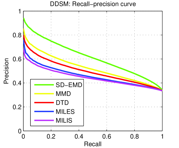
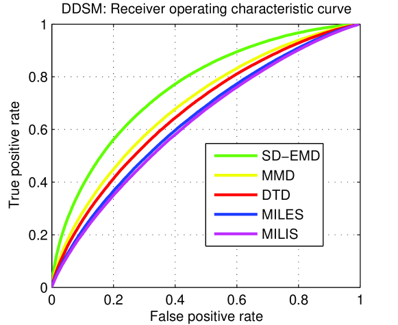
Figure 1: Experimental results over the DDSM data set.

4.5 Results over the SemEval-2010 Task 8 data set

The recall-precision curve and the receiver operating characteristic curve of the experiments over the SemEval-2010 Task 8 data set are shown in 2. Again, we observed that the proposed method, SD-EMD, outperforms all the compared methods over the SemEval-2010 Task 8 data set. This means that the proposed EMD based dictionary learning method not only works well over the medical image data, but also has good performances over the natural language processing problems.

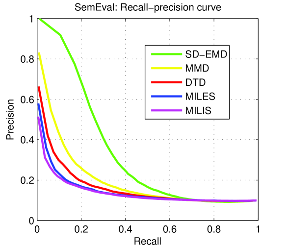
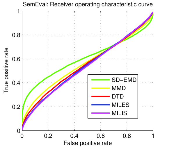
Figure 2: Experimental results over the SemEval-2010 Task 8 data set.

5 Conclusions

In this paper, we discuss the problem of representing multi-instance data sample by using the dictionary. The bags of instances are represented as histograms and the EMD is used to compare histograms. In this paper, for the first time, we proposed to learn EMD-optimal dictionary. We proposed a novel learning framework to train the dictionary by using the stochastic optimization method. The proposed method shows its advantage over the existing dictionary learning methods.

6 Future works

In this paper, we use the large margin as the loss function to model the problem. In the future, we will consider using more complex loss functions of multivariate performance measures liang2016optimizing ; lin2016multi ; wang2015multiple ; fan2010enhanced . Moreover, we will also consider using Bayesian network to represent the histograms and learn the parameters of Bayesian network for EMD based comparison fan2014tightening ; fan2014finding ; fan2015improved . In the future, we will also applied the proposed method to various applications, including multimedia technology wang2014effective ; wang2015supervised ; liu2015supervised ; liang2016novel , information security xu2013cross ; xu2014adaptive ; xu2014evasion ; xu2012push , computer vision wang2015deeply ; wang2013can ; wang2013gender ; wang2014leveraging , medical imaging li2015outlier ; li2015burn ; mo2015importance ; king2015surgical , etc.

References

- (1) Beecks, C., Uysal, M., Seidl, T.: Earth mover’s distance vs. quadratic form distance: An analytical and empirical comparison. In: Proceedings - 2015 IEEE International Symposium on Multimedia, ISM 2015, pp. 233–236 (2016)
- (2) Chen, T.C., Chen, Y.Y., Ma, T.C., Chen, L.G.: Design and implementation of cubic spline interpolation for spike sorting microsystems. In: 2011 IEEE International Conference on Acoustics, Speech and Signal Processing (ICASSP), pp. 1641–1644. IEEE (2011)
- (3) Chen, T.C., Ma, T.C., Chen, Y.Y., Chen, L.G.: Low power and high accuracy spike sorting microprocessor with on-line interpolation and re-alignment in 90nm cmos process. In: 2012 Annual International Conference of the IEEE Engineering in Medicine and Biology Society, pp. 4485–4488. IEEE (2012)
- (4) Chen, T.T., Liu, C., Ding, X.M., Zou, H., Shen, Q., Liu, Y.: A multi-instance multi-label learning algorithm based on feature selection. In: Proceedings - 2015 10th International Conference on Broadband and Wireless Computing, Communication and Applications, BWCCA 2015, pp. 587–590 (2016)
- (5) Chen, Y., Bi, J., Wang, J.Z.: Miles: Multiple-instance learning via embedded instance selection. Pattern Analysis and Machine Intelligence, IEEE Transactions on 28(12), 1931–1947 (2006)
- (6) Chen, Y.H., Chen, T.C., Ma, T.C., Lee, T.H., Chen, L.G., et al.: Sub-microwatt knn classifier for implantable closed-loop epileptic neuromodulation system. In: Proceedings of the 2009 International Symposium on Bioelectronics and Bioinformatics, p. 13. RMIT University, School of Electrical and Computer Engineering (2009)
- (7) Clarkson, E., Cushing, J.: Shannon information and receiver operating characteristic analysis for multiclass classification in imaging. Journal of the Optical Society of America A: Optics and Image Science, and Vision 33(5), 930–937 (2016)
- (8) Fan, X., Malone, B., Yuan, C.: Finding optimal bayesian network structures with constraints learned from data. In: Proceedings of the 30th annual conference on uncertainty in artificial intelligence (UAI-14), pp. 200–209 (2014)
- (9) Fan, X., Tang, K.: Enhanced maximum auc linear classifier. In: Fuzzy Systems and Knowledge Discovery (FSKD), 2010 Seventh International Conference on, vol. 4, pp. 1540–1544. IEEE (2010)
- (10) Fan, X., Yuan, C.: An improved lower bound for bayesian network structure learning. In: AAAI, pp. 3526–3532 (2015)
- (11) Fan, X., Yuan, C., Malone, B.M.: Tightening bounds for bayesian network structure learning. In: AAAI, pp. 2439–2445. Citeseer (2014)
- (12) Fu, Z., Robles-Kelly, A., Zhou, J.: Milis: Multiple instance learning with instance selection. Pattern Analysis and Machine Intelligence, IEEE Transactions on 33(5), 958–977 (2011)
- (13) Goadrich, M., Oliphant, L., Shavlik, J.: Gleaner: Creating ensembles of first-order clauses to improve recall-precision curves. Machine Learning 64(1-3), 231–261 (2006)
- (14) Hendrickx, I., Kim, S.N., Kozareva, Z., Nakov, P., Ó Séaghdha, D., Padó, S., Pennacchiotti, M., Romano, L., Szpakowicz, S.: Semeval-2010 task 8: Multi-way classification of semantic relations between pairs of nominals. In: Proceedings of the Workshop on Semantic Evaluations: Recent Achievements and Future Directions, pp. 94–99. Association for Computational Linguistics (2009)
- (15) Huo, J., Gao, Y., Yang, W., Yin, H.: Abnormal event detection via multi-instance dictionary learning. Lecture Notes in Computer Science (including subseries Lecture Notes in Artificial Intelligence and Lecture Notes in Bioinformatics) 7435 LNCS, 76–83 (2012)
- (16) Huo, J., Gao, Y., Yang, W., Yin, H.: Multi-instance dictionary learning for detecting abnormal events in surveillance videos. International Journal of Neural Systems 24(3), 1430,010 (2014)
- (17) Ju, C.C., Liu, T.M., Chen, Y.H., Lee, K.B., Cheng, C.Y., Chao, H.T., Wang, C.M., Wu, T.H., Lin, T.A., Chou, H.L., et al.: A 1.94 mm 2, 38.17 mw dual vp8/h. 264 full-hd encoder/decoder lsi for social network services (sns) over smart-phones. In: Solid State Circuits Conference (A-SSCC), 2012 IEEE Asian, pp. 13–16. IEEE (2012)
- (18) Kim, M., Han, D., Ko, H.: Joint patch clustering-based dictionary learning for multimodal image fusion. Information Fusion 27, 198–214 (2016)
- (19) King, D.R., Li, W., Squiers, J.J., Mohan, R., Sellke, E., Mo, W., Zhang, X., Fan, W., DiMaio, J.M., Thatcher, J.E.: Surgical wound debridement sequentially characterized in a porcine burn model with multispectral imaging. Burns 41(7), 1478–1487 (2015)
- (20) Li, J.Y., Li, J.H., Shui-Cheng, Y.: Multi-instance learning using information entropy theory for image retrieval. In: Proceedings - 17th IEEE International Conference on Computational Science and Engineering, CSE 2014, Jointly with 13th IEEE International Conference on Ubiquitous Computing and Communications, IUCC 2014, 13th International Symposium on Pervasive Systems, Algorithms, and Networks, I-SPAN 2014 and 8th International Conference on Frontier of Computer Science and Technology, FCST 2014, pp. 1727–1733 (2015)
- (21) Li, W., Mo, W., Zhang, X., Lu, Y., Squiers, J.J., Sellke, E.W., Fan, W., DiMaio, J.M., Thatcher, J.E.: Burn injury diagnostic imaging device’s accuracy improved by outlier detection and removal. In: SPIE Defense+ Security, pp. 947,206–947,206. International Society for Optics and Photonics (2015)
- (22) Li, W., Mo, W., Zhang, X., Squiers, J.J., Lu, Y., Sellke, E.W., Fan, W., DiMaio, J.M., Thatcher, J.E.: Outlier detection and removal improves accuracy of machine learning approach to multispectral burn diagnostic imaging. Journal of biomedical optics 20(12), 121,305–121,305 (2015)
- (23) Liang, R.Z., Shi, L., Wang, H., Meng, J., Wang, J.J.Y., Sun, Q., Gu, Y.: Optimizing Top Precision Performance Measure of Content-Based Image Retrieval by Learning Similarity Function. In: Pattern Recognition (ICPR), 2016 23st International Conference on. IEEE (2016)
- (24) Liang, R.Z., Xie, W., Li, W., Wang, H., Wang, J.J.Y., Taylor, L.: A novel transfer learning method based on common space mapping and weighted domain matching. In: Tools with Artificial Intelligence (ICTAI), 2016 IEEE 28th International Conference on. IEEE (2016)
- (25) Lin, F., Wang, J., Zhang, N., Xiahou, J., McDonald, N.: Multi-kernel learning for multivariate performance measures optimization. Neural Computing and Applications pp. 1–13 (2016)
- (26) Liu, X., Wang, J., Yin, M., Edwards, B., Xu, P.: Supervised learning of sparse context reconstruction coefficients for data representation and classification. Neural Computing and Applications pp. 1–9 (2015)
- (27) Lobel, H., Vidal, R., Soto, A.: Learning shared, discriminative, and compact representations for visual recognition. IEEE Transactions on Pattern Analysis and Machine Intelligence 37(11), 2218–2231 (2015)
- (28) Ma, T.C., Chen, T.C., Chen, L.G.: Design and implementation of a low power spike detection processor for 128-channel spike sorting microsystem. In: 2014 IEEE International Conference on Acoustics, Speech and Signal Processing (ICASSP), pp. 3889–3892. IEEE (2014)
- (29) Mo, W., Mohan, R., Li, W., Zhang, X., Sellke, E.W., Fan, W., DiMaio, J.M., Thatcher, J.E.: The importance of illumination in a non-contact photoplethysmography imaging system for burn wound assessment. In: SPIE BiOS, pp. 93,030M–93,030M. International Society for Optics and Photonics (2015)
- (30) Nabavi, S., Beck, A.: Earth mover’s distance for differential analysis of heterogeneous genomics data. In: 2015 IEEE Global Conference on Signal and Information Processing, GlobalSIP 2015, pp. 963–966 (2016)
- (31) Rose, C., Turi, D., Williams, A., Wolstencroft, K., Taylor, C.: Web services for the ddsm and digital mammography research. Lecture Notes in Computer Science (including subseries Lecture Notes in Artificial Intelligence and Lecture Notes in Bioinformatics) 4046 LNCS, 376–383 (2006)
- (32) Shao, Z., Er, M.: Efficient leave-one-out cross-validation-based regularized extreme learning machine. Neurocomputing 194, 260–270 (2016)
- (33) Tong, J., Schreier, P., Guo, Q., Tong, S., Xi, J., Yu, Y.: Shrinkage of covariance matrices for linear signal estimation using cross-validation. IEEE Transactions on Signal Processing 64(11), 2965–2975 (2016)
- (34) Vanwinckelen, G., Tragante do O, V., Fierens, D., Blockeel, H.: Instance-level accuracy versus bag-level accuracy in multi-instance learning. Data Mining and Knowledge Discovery 30(2), 313–341 (2016)
- (35) Wang, D., Attwood, K., Tian, L.: Receiver operating characteristic analysis under tree orderings of disease classes. Statistics in Medicine 35(11), 1907–1926 (2016)
- (36) Wang, H., Wang, J.: An effective image representation method using kernel classification. In: 2014 IEEE 26th International Conference on Tools with Artificial Intelligence (ICTAI 2014), pp. 853–858 (2014)
- (37) Wang, J., Wang, H., Zhou, Y., McDonald, N.: Multiple kernel multivariate performance learning using cutting plane algorithm. In: Systems, Man, and Cybernetics (SMC), 2015 IEEE International Conference on, pp. 1870–1875. IEEE (2015)
- (38) Wang, J., Zhou, Y., Duan, K., Wang, J.J.Y., Bensmail, H.: Supervised cross-modal factor analysis for multiple modal data classification. In: Systems, Man, and Cybernetics (SMC), 2015 IEEE International Conference on, pp. 1882–1888. IEEE (2015)
- (39) Wang, K., Liu, J., González, D.: Domain transfer multi-instance dictionary learning. Neural Computing and Applications pp. 1–10 (2016)
- (40) Wang, X., Guo, R., Kambhamettu, C.: Deeply-learned feature for age estimation. In: 2015 IEEE Winter Conference on Applications of Computer Vision, pp. 534–541. IEEE (2015)
- (41) Wang, X., Kambhamettu, C.: Gender classification of depth images based on shape and texture analysis. In: Global Conference on Signal and Information Processing (GlobalSIP), 2013 IEEE, pp. 1077–1080. IEEE (2013)
- (42) Wang, X., Kambhamettu, C.: Leveraging appearance and geometry for kinship verification. In: 2014 IEEE International Conference on Image Processing (ICIP), pp. 5017–5021. IEEE (2014)
- (43) Wang, X., Ly, V., Lu, G., Kambhamettu, C.: Can we minimize the influence due to gender and race in age estimation? In: Machine Learning and Applications (ICMLA), 2013 12th International Conference on, vol. 2, pp. 309–314. IEEE (2013)
- (44) Wang, X., Wang, B., Bai, X., Liu, W., Tu, Z.: Max-margin multiple-instance dictionary learning. In: Proceedings of the 30th International Conference on Machine Learning, pp. 846–854 (2013)
- (45) Wu, J.H., Tang, L.B., Zhao, B.J., Deng, C.W., Li, J.T.: Visual dictionary and online multi-instance learning based object tracking. Xi Tong Gong Cheng Yu Dian Zi Ji Shu/Systems Engineering and Electronics 37(2), 428–435 (2015)
- (46) Xia, H., Hoi, S., Jin, R., Zhao, P.: Online multiple kernel similarity learning for visual search. IEEE Transactions on Pattern Analysis and Machine Intelligence 36(3), 536–549 (2014)
- (47) Xu, L., Zhan, Z., Xu, S., Ye, K.: Cross-layer detection of malicious websites. In: Proceedings of the third ACM conference on Data and application security and privacy, pp. 141–152. ACM (2013)
- (48) Xu, L., Zhan, Z., Xu, S., Ye, K.: An evasion and counter-evasion study in malicious websites detection. In: Communications and Network Security (CNS), 2014 IEEE Conference on, pp. 265–273. IEEE (2014)
- (49) Xu, M., Dong, H., Chen, C., Li, L.: Unsupervised dictionary learning with fisher discriminant for clustering. Neurocomputing 194, 65–73 (2016)
- (50) Xu, S., Lu, W., Xu, L.: Push-and pull-based epidemic spreading in networks: Thresholds and deeper insights. ACM Transactions on Autonomous and Adaptive Systems (TAAS) 7(3), 32 (2012)
- (51) Xu, S., Lu, W., Xu, L., Zhan, Z.: Adaptive epidemic dynamics in networks: Thresholds and control. ACM Transactions on Autonomous and Adaptive Systems (TAAS) 8(4), 19 (2014)
- (52) Yan, Z., Zhan, Y., Peng, Z., Liao, S., Shinagawa, Y., Zhang, S., Metaxas, D., Zhou, X.: Multi-instance deep learning: Discover discriminative local anatomies for bodypart recognition. IEEE Transactions on Medical Imaging 35(5), 1332–1343 (2016)
- (53) Ying, P., Liu, J., Lu, H.: Dictionary learning based superpixels clustering for weakly-supervised semantic segmentation. In: Proceedings - International Conference on Image Processing, ICIP, vol. 2015-December, pp. 4258–4262 (2015)
- (54) Zhang, M., Peng, J., Liu, X.: Sparse coding with earth mover’s distance for multi-instance histogram representation. Neural Computing and Applications pp. 1–12 (2016)
- (55) Zhang, P., Su, W.: Statistical inference on recall, precision and average precision under random selection. In: Proceedings - 2012 9th International Conference on Fuzzy Systems and Knowledge Discovery, FSKD 2012, pp. 1348–1352 (2012)