Information Content of Greedy
MaxCut  Algorithms

Greedy MaxCut  Algorithms
and their Information Content

Abstract

MaxCut defines a classical NP-hard problem for graph partitioning and it serves as a typical case of the symmetric non-monotone Unconstrained Submodular Maximization (USM) problem. Applications of MaxCut are abundant in machine learning, computer vision and statistical physics. Greedy algorithms to approximately solve MaxCut rely on greedy vertex labelling or on an edge contraction strategy. These algorithms have been studied by measuring their approximation ratios in the worst case setting but very little is known to characterize their robustness to noise contaminations of the input data in the average case. Adapting the framework of Approximation Set Coding, we present a method to exactly measure the cardinality of the algorithmic approximation sets of five greedy MaxCut algorithms. Their information contents are explored for graph instances generated by two different noise models: the edge reversal model and Gaussian edge weights model. The results provide insights into the robustness of different greedy heuristics and techniques for MaxCut, which can be used for algorithm design of general USM problems.

I Introduction

Algorithms are mostly analyzed by measuring their runtime and memory consumption for the worst possible input instance. In many application scenarios, algorithms are also selected according to their “robustness” to noise perturbations of the input instance and their insensitivity to randomization during algorithm execution. How should this “robustness” property be measured? Machine learning requires that algorithms with random variables as input generalize over these fluctuations. The algorithmic answer has to be stable w.r.t. this uncertainty in the input instance. Approximation Set Coding (ASC) quantifies the impact of input randomness on the solution space of an algorithm by measuring the attainable resolution for the algorithm’s output. We employ this framework in an exemplary way by estimating the robustness of MaxCut algorithms to specific input instances. Thereby, we effectively perform an average case analysis of the generalization properties of MaxCut algorithms.

I-A MaxCut  and Unconstrained Submodular Maximization

Given an undirected graph $G=(V,E)$ with vertex set $V=\{v_{1},v_{2},\cdots,v_{n}\}$ and edge set $E$ with nonnegative weights $w_{ij},\forall(i,j)\in E$, the MaxCut  problem aims to find a partition of vertices into two disjoint subsets $S_{1}$ and $S_{2}$, such that the cut value $cut(S_{1},S_{2}):=\sum_{i\in S_{1}}\sum_{j\in S_{2}}w_{ij}$ is maximized. MaxCut is emlpoyed in various applications, such as in semisupervised learning ([1]), in social network ([2]), in statistical physics and in circuit layout design ([3]). MaxCut is considered to be a typical case of the USM problem because its objective can be formulated as a set function: $f(S):=cut(S,V\backslash S),S\subseteq V$, which is submodular, nonmonotone, and symmetric ($f(S)=f(V\backslash S)$). Beside MaxCut, USM captures many practical problems such as MaxDiCut ([4]), variants of MaxSat and the maximum facility location problem ([5, 6]).

I-B Greedy Heuristics and Techniques

The five algorithms investigated here (as summarized in Table I) belong to two greedy heuristics: double greedy and backward greedy. The double greedy algorithms exploit the symmetric property of USM, and conducts classical forward greedy and backward greedy simultaneously: it works on two solutions initialized as $\emptyset$ and the ground set $V$, respectively, then processes the elements (vertices for MaxCut problem) one at a time, for which it determines whether it should be added to the first solution or removed from the second solution. The backward greedy algorithm removes the smallest weighted edge in each step. The difference of the four double greedy algorithms lies in the greedy techniques they use: sorting, randomization and the way to initialize the first two vertices.

I-C Approximation Set Coding for Algorithm Analysis

In analogy to Shannon’s theory of communication, the ASC framework ([7], [8], [9]) determines distinguishable sets of solutions and, thereby, provides a general principle to conduct model validation ([10], [11]). As an algorithmic variant of the ASC framework, [12, 13] defines the algorithmic $t$-approximation set of an algorithm $\mathscr{A}$ at step $t$ as the set of feasible solutions after $t$ steps, $C_{t}^{\mathscr{A}}(G):=A_{t}(G)$, where $A_{t}(G)$ is the solution set which are still considered as viable by $\mathscr{A}$ after $t$ computational steps.

ASC utilizes the two instance-scenario to investigate the information content of greedy MaxCut algorithms. Since we investigate the average case behavior of algorithms, we have to specify the probability distribution of the input instances. We generate graph instances in a two step process. First, generate a “master graph” $G$, e.g., a complete graph with Gaussian distributed weights. In a second step, we generate two input graphs $G^{\prime},\;G^{\prime\prime}$ by independently applying a noise process to edge weights of the master graph $G$.

The algorithmic analogy of information content ([7]), i.e. algorithmic information content $I^{\mathscr{A}}$, is computed as the maximum stepwise information $I_{t}^{\mathscr{A}}$:

$$I^{\mathscr{A}}:=\max_{t}I_{t}^{\mathscr{A}}=\max_{t}\mathbb{E}\Bigl{[}\log\Bigl{(}\frac{|{\cal C}|\;\Delta_{t}^{\mathscr{A}}(G^{\prime},G^{\prime\prime})}{|C_{t}^{\mathscr{A}}(G^{\prime})||C_{t}^{\mathscr{A}}(G^{\prime\prime})|}\Bigr{)}\Bigr{]}$$ (1)

The expectation is taken w.r.t. ($G^{\prime}$, $G^{\prime\prime}$); $\Delta_{t}^{\mathscr{A}}(G^{\prime},G^{\prime\prime}):=|C_{t}^{\mathscr{A}}(G^{\prime})\cap C_{t}^{\mathscr{A}}(G^{\prime\prime})|$ denotes the intersection of approximation sets, and ${\cal C}$ is the solution space, i.e., all possible cuts. The information content $I^{\mathscr{A}}_{t}$ measures how much information is extracted by algorithm ${\mathscr{A}}$ at iteration $t$ from the input distribution that is relevant to the output distribution.

TABLE I: Summary of Greedy MaxCut  Algorithms

Name	Greedy	Techniques
	Heuristic	Sort.	Rand.	Init. Vertices
D2Greedy	Double
RDGreedy			$\checkmark$
SG				$\checkmark$
SG3		$\checkmark$		$\checkmark$
EC	Backward	$\checkmark$

II Greedy MaxCut  Algorithms

We investigate five greedy algorithms (Table I) for MaxCut. According to the type of greedy heuristic, they can be divided into two categories: I) Double Greedy: SG, SG3, D2Greedy, RDGreedy; II) Backward Greedy: Edge Contraction. Besides the type of greedy heuristic, the difference between the algorithms are mainly in three techniques: sorting the candidate elements, randomization and the way initializing the first two vertices. In the following, we briefly introduce one typical algorithm in each category and we present the others by showing the difference (details are in the Supplement VI-A because of space limit).

II-A Double Greedy Algorithms

D2Greedy (Alg. 1) is the Deterministic double greedy, RDGreedy is the Randomized double greedy, they were proposed by [14] to solve the general USM problem with ${1/3}$ and ${1/2}$ worst-case approximation guarantee, respectively. They use the same double greedy heuristic as SG ([15]) and SG3 (variant of SG), which are classical greedy MaxCut algorithms. We prove in Supplement VI-B that, for MaxCut, SG and D2Greedy use equivalent labelling criteria except for initializing the first two vertices.

Input: Complete graph $G=(V,E)$ with nonnegative edges

Output: A disjoint cut and the cut value

1 $S^{0}:=\emptyset$, $T^{0}:=V$;

2 for $i=1$ to $n$ do

3       $a^{i}:=f(S^{i-1}\cup\{v_{i}\})-f(S^{i-1})$;

4       $b^{i}:=f(T^{i-1}\backslash\{v_{i}\})-f(T^{i-1})$;

5       if $a^{i}\geq b^{i}$ then

            $S^{i}:=S^{i-1}\cup\{v_{i}\}$, $T^{i}:=T^{i-1}$ ;

              // expand $S$

6            

7      else

            $S^{i}:=S^{i-1}$, $T^{i}:=T^{i-1}\backslash\{v_{i}\}$ ;

              // shrink $T$

8            

9      

return $S^{n}$, $V\backslash S^{n}$, and $cut(S^{n},V\backslash S^{n})$

Algorithm 1 D2Greedy ([14])

As shown in Alg. 1, D2Greedy maintains two solution sets: $S$ initialized as $\emptyset$, $T$ initialized as the ground set $V$. It labels all the vertices one by one: for vertex $v_{i}$, it computes the objective gain of adding $v_{i}$ to $S$ and the gain of removing $v_{i}$ from $T$, then labels $v_{i}$ to have higher objective gain.

SG and D2Greedy differ in the initialization of the first two vertices: SG picks first of all the maximum weighted edge and distributes its two vertices to the two active subsets. Compared to D2Greedy, the RDGreedy uses randomization technique when labelling each vertex: it labels each vertex with probability proportional to the objective gain. Compared to SG, SG3 sorts the unlabelled vertices according to a certain score function (which is proportional to the possible objective gains), and selects the vertex with the maximum score to be the next one to be labelled.

II-B Edge Contraction (EC)

EC ([16], Alg. 2) contracts the smallest edge in each step. The two vertices of this contracted edge become one “super” vertex, and the weight of an edge connecting this super vertex to any other vertex is assigned as the sum of weights of the original two edges. EC belongs to the backward greedy in the sense that it tries to remove the least expensive edge from the cut set in each step. We can easily derive a heuristic for the Max-k-Cut problem by using $n-k$ steps instead of $n-2$ steps.

Input: Complete graph $G=(V,E)$ with nonnegative edge

Output: A disjoint cut $S_{1},S_{2}$ and cut value $cut(S_{1},S_{2})$

1 for $i=1:n$ do

2      $ContractionList(i):=\{i\}$;

3for $i=1:n-2$ do

4       Find a minimum weight edge $(x,y)$ in $G$;

       $v:=contract(x,y)$, $V:=V\cup\{v\}\backslash\{x,y\}$ ;

        // contract

5       for $j\in V\backslash\{v\}$ do

6            $w_{vj}:=w_{xj}+w_{yj}$;

7      $ContractionList(v):=ContractionList(x)\cup ContractionList(y)$;

8      

9Denote by $x$ and $y$ the only 2 vertices in $V$;

return $S_{1}:=ContractionList(x)$, $S_{2}:=ContractionList(y)$, $cut(S_{1},S_{2}):=w_{xy}$

Algorithm 2 Edge Contraction (EC) ([16])

III Counting Solutions in Approximation Sets

To compute the information content according to Eq. 1, we need to exactly compute the cardinalities of four different solution sets. For MaxCut problem, the solution space has the cardinality $|{\cal C}|=2^{n-1}-1$. In the following we will present guaranteed methods for exact counting $|C_{t}^{\mathscr{A}}(G^{\prime})|,|C_{t}^{\mathscr{A}}(G^{\prime\prime})|$ and $\Delta_{t}^{\mathscr{A}}(G^{\prime},G^{\prime\prime})$ (sub-/superscripts omitted for notational clarity).

III-A Counting Methods for Double Greedy Algorithms

The counting methods for the double greedy algorithms are similar, so we only discuss the method for SG3 here; details about other methods and the corresponding proofs are in the Supplement VI-C and VI-D, respectively.

For the SG3 (Alg. 6, see Supplement), after step $t$ ($t=1,\cdots,n-1$) there are $k=n-t-1$ unlabelled vertices, and it is clear that $|C(G^{\prime})|=|C(G^{\prime\prime})|=2^{k}$.

To count the intersection set $\Delta(G^{\prime},G^{\prime\prime})$, assume the solution set pair of $G^{\prime}$ is $(S_{1}^{\prime},S_{2}^{\prime})$, the solution set pair of $G^{\prime\prime}$ is $(S_{1}^{\prime\prime},S_{2}^{\prime\prime})$, so the unlabelled vertex sets are $T^{\prime}=V\backslash\{S_{1}^{\prime}\cup S_{2}^{\prime}\}$, $T^{\prime\prime}=V\backslash\{S_{1}^{\prime\prime}\cup S_{2}^{\prime\prime}\}$, respectively. Denote $L:=T^{\prime}\cap T^{\prime\prime}$ be the common vertices of the two unlabelled vertex sets, so $l=|L|$ ($0\leq l\leq k$) is the number of common vertices in the unlabelled $k$ vertices. Denote $M^{\prime}:=T^{\prime}\backslash L$, $M^{\prime\prime}:=T^{\prime\prime}\backslash L$ be the sets of different vertex sets between the two unlabelled vertex sets. Then,

$$\Delta(G^{\prime},G^{\prime\prime})=\left\{\begin{array}[]{ll}\hbox{\multirowsetup$2^{l}$}&\textrm{if $(S_{1}^{\prime\prime}\backslash M^{\prime},S_{2}^{\prime\prime}\backslash M^{\prime})$ is matched by}\\ &\textrm{$(S_{1}^{\prime}\backslash M^{\prime\prime},S_{2}^{\prime}\backslash M^{\prime\prime})$ or $(S_{2}^{\prime}\backslash M^{\prime\prime},S_{1}^{\prime}\backslash M^{\prime\prime})$}\\ 0&\textrm{otherwise}\\ \end{array}\right.$$

III-B Counting Method for Edge Contraction Algorithm

For EC (Alg. 2), after step $t$ ($t=1,\cdots,n-2$) there are $k=n-t$ “super” vertices (i.e. contracted ones). It is straightforward to see that $|C(G^{\prime})|=|C(G^{\prime\prime})|=2^{k-1}-1$.

To count the intersection $\Delta(G^{\prime},G^{\prime\prime})$, suppose there are $l$ ($0\leq l\leq k$) common super vertices in the unlabelled $k$ vertices. Remove the $l$ common super vertices from each set, then there are $h=k-l$ distinct super vertices in each set, denote them by $P:=\{\mathbf{p}_{1},\mathbf{p}_{2},\cdots,\mathbf{p}_{h}\}$, $Q:=\{\mathbf{q}_{1},\mathbf{q}_{2},\cdots,\mathbf{q}_{h}\}$, respectively. Notice that $\mathbf{p}_{1}\cup\mathbf{p}_{2}\cup\cdots\cup\mathbf{p}_{h}=\mathbf{q}_{1}\cup\mathbf{q}_{2}\cup\cdots\cup\mathbf{q}_{h}$, so after some contractions in both $P$ and $Q$, there must be some common super vertices between $P$ and $Q$. Assume the maximum number of common super vertices after all possible contractions is $c^{*}$, then it holds

$$\Delta(G^{\prime},G^{\prime\prime})=2^{c^{*}+l-1}-1\;.$$ (2)

To compute $c^{*}$, we propose a polynomial time algorithm (Alg. 3) with a theoretical guarantee in Theorem 1 (for the proof see Supplement VI-E). The algorithm finds the maximal number of common super vertices after all possible contractions, that is used to count $\Delta(G^{\prime},G^{\prime\prime})$ for EC.

Theorem 1.

Given two distinct super vertex sets $P:=\{\mathbf{p}_{1},\mathbf{p}_{2},\cdots,\mathbf{p}_{h}\}$, $Q:=\{\mathbf{q}_{1},\mathbf{q}_{2},\cdots,\mathbf{q}_{h}\}$ (any 2 super vertices inside $P$ or $Q$ do not intersect, and there is no common super vertex between $P$ and $Q$), such that $\mathbf{p}_{1}\cup\mathbf{p}_{2}\cup\cdots\cup\mathbf{p}_{h}=\mathbf{q}_{1}\cup\mathbf{q}_{2}\cup\cdots\cup\mathbf{q}_{h}$, Alg. 3 returns the maximum number of common super vertices between $P$ and $Q$ after all possible contractions.

Input: Two distinct super vertex sets $P$, $Q$

Output: Maximum number of common super vertices after all possible contractions

1 $c:=0$;

2 while $P\neq\emptyset$ do

3       Randomly pick $\mathbf{p}_{i}\in P$;

4       Find $\mathbf{q}_{j}\in Q$ s.t. $\mathbf{p}_{i}\cap\mathbf{q}_{j}\neq\emptyset$;

5       if $\mathbf{q}_{j}\backslash\mathbf{p}_{i}\neq\emptyset$ then

6             For $\mathbf{p}_{i}$, find $\mathbf{p}_{i^{\prime}}\in P\backslash\{\mathbf{p}_{i}\}$ s.t. $\mathbf{p}_{i^{\prime}}\cap(\mathbf{q}_{j}\backslash\mathbf{p}_{i})\neq\emptyset$;

7             $\mathbf{p_{ii^{\prime}}}:=\mathbf{p}_{i}\cup\mathbf{p}_{i^{\prime}}$, $P:=P\cup\{\mathbf{p_{ii^{\prime}}}\}\backslash\{\mathbf{p}_{i},\mathbf{p}_{i^{\prime}}\}$ ;

8            

9      if $\mathbf{p}_{i}\backslash\mathbf{q}_{j}\neq\emptyset$ then

10             For $\mathbf{q}_{j}$, find $\mathbf{q}_{j^{\prime}}\in Q\backslash\{\mathbf{q}_{j}\}$ s.t. $\mathbf{q}_{j^{\prime}}\cap(\mathbf{p}_{i}\backslash\mathbf{q}_{j})\neq\emptyset$;

11             $\mathbf{q_{jj^{\prime}}}:=\mathbf{q}_{j}\cup\mathbf{q}_{j^{\prime}}$, $Q:=Q\cup\{\mathbf{q_{jj^{\prime}}}\}\backslash\{\mathbf{q}_{j},\mathbf{q}_{j^{\prime}}\}$ ;

12            

13      if $\mathbf{p_{ii^{\prime}}}==\mathbf{q_{jj^{\prime}}}$ then

14             Remove $\mathbf{p_{ii^{\prime}}}$, $\mathbf{q_{jj^{\prime}}}$ from $P$, $Q$, respectively;

15             $c:=c+1$;

16            

17      

return $c$

Algorithm 3 Common Super Vertex Counting

IV Experiments

We conducted experiments on two exemplary models: the edge reversal model and the Gaussian edge weights model. Each model involves the master graph $G$ and a noise type used to generate the two noisy instances $G^{\prime}$ and $G^{\prime\prime}$. The width of the instance distribution is controlled by the strength of the noise model. These models provide the setting to investigate the algorithmic behavior.

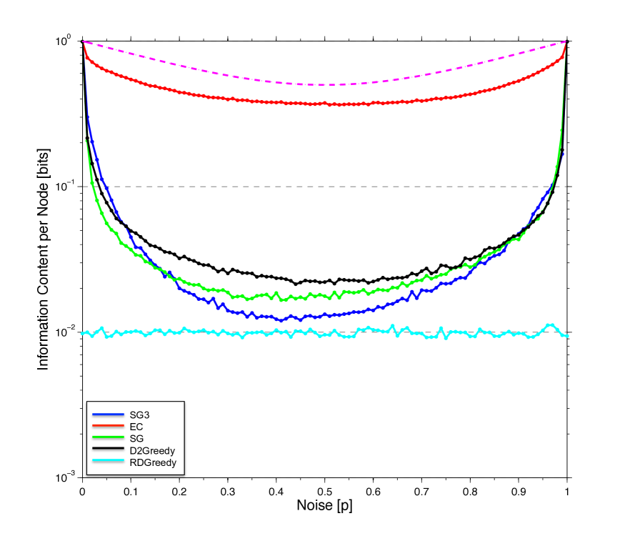
(a) Edge Reversal Model, $n$: 100

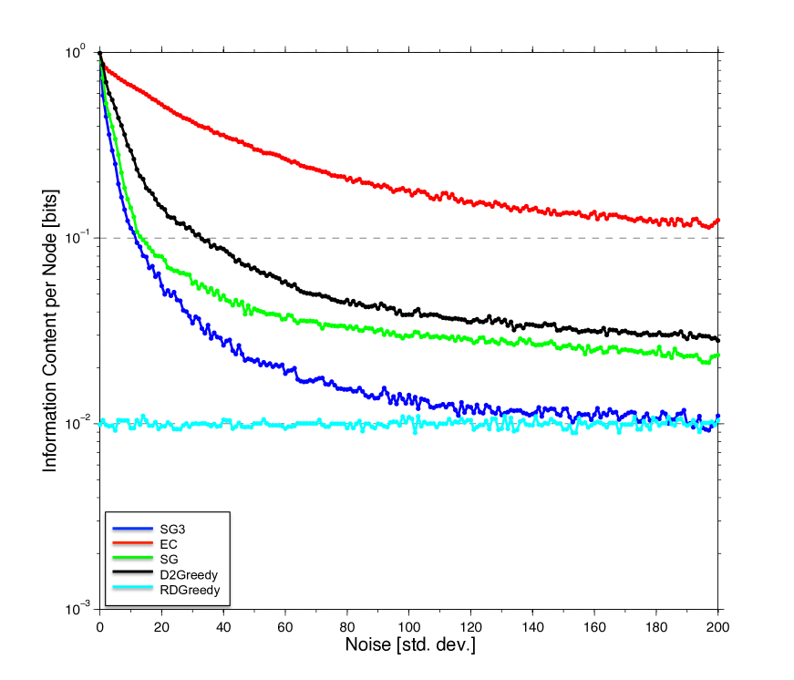
(b) Gaussian Edge Weights Model, $n$: 100

Figure 1: Information Content per Node

IV-A Experimental Setting

Edge Reversal Model: To obtain the master graph, we generate a balanced bipartite graph $G_{b}$ with disjoint vertex sets $S_{1}$, $S_{2}$. Then we assign uniformly distributed weights in $[0,\frac{8}{n^{2}}]$ to all edges inside $S_{1}$ or $S_{2}$ and we assign uniformly distributed weights in $[1-\frac{8}{n^{2}},1]$ to all edges between $S_{1}$ and $S_{2}$, thus generating graph $G^{\prime}_{b}$. Then randomly flip edges in $G^{\prime}_{b}$ to generate the master graph $G$. Here, flip edge $e_{ij}$ means changing its weight $w_{ij}$ to $1-w_{ij}$ with probability $p_{m}$, and $(flip\;e_{ij})\sim Ber(p_{m})$; $p_{m}=0.2$ is used to generate the master graph $G$. Noisy graphs $G^{\prime}$, $G^{\prime\prime}$ are generated by flipping the edges in $G$ with probability $p$, ($(flip\;e_{ij})\sim Ber(p)$).

Gaussian Edge Weights Model: The master graph $G$ is generated with Gaussian distributed edge weights $w_{ij}\sim N(\mu,\sigma_{m}^{2})$, $\mu=600,\sigma_{m}=50$, negative edges are set to be $\mu$. Noisy graphs $G^{\prime}$, $G^{\prime\prime}$ are obtained by adding Gaussian distributed noise $n_{ij}\sim N(0,\sigma^{2})$, negative noisy edges are set to be 0.

For both noise models, we conducted 1000 experiments on i.i.d. generated noisy graphs $G^{\prime}$ and $G^{\prime\prime}$, and then we aggregate the results to estimate the expectation in Eq. 1.

IV-B Results

We plot the information content and stepwise information per node in Fig.  1 and  2, respectively. For the edge reversal model, we also investigate the number of equal edge pairs between $G^{\prime}$ and $G^{\prime\prime}$: $d=0,\cdots,m$ ($m$ is the total edge number), $d$ measures the consistency of the two noisy instances. The expected fraction of equal edge pairs is $\mathbb{E}d=p^{2}+(1-p)^{2}$, and it is plotted as the dashed magenta line in Fig.  1(a).

IV-C Analysis

Before discussing these results, let us revisit the stepwise information and information content. From the counting methods in Section III, we derive the analytical form of $|{\cal C}|$, $|C_{t}^{\mathscr{A}}(G^{\prime})|$ and $|C_{t}^{\mathscr{A}}(G^{\prime\prime})|$ (e.g., $\mathscr{A}=SG3$), an we insert these values into the definition of stepwise information,

$$I_{t}^{\mathscr{A}}=\mathbb{E}\log\Bigl{(}|{\cal C}|\frac{\Delta_{t}^{\mathscr{A}}(G^{\prime},G^{\prime\prime})}{|C_{t}^{\mathscr{A}}(G^{\prime})||C_{t}^{\mathscr{A}}(G^{\prime\prime})|}\Bigr{)}$$ (3)

$$=\mathbb{E}(\log(|{\cal C}|\Delta_{t}^{\mathscr{A}}(G^{\prime},G^{\prime\prime}))-\log(|C_{t}^{\mathscr{A}}(G^{\prime})||C_{t}^{\mathscr{A}}(G^{\prime\prime})|))$$

$$=\mathbb{E}\log\Delta_{t}^{\mathscr{A}}(G^{\prime},G^{\prime\prime})+2t+\log(2^{n-1}-1)-2(n-1)$$

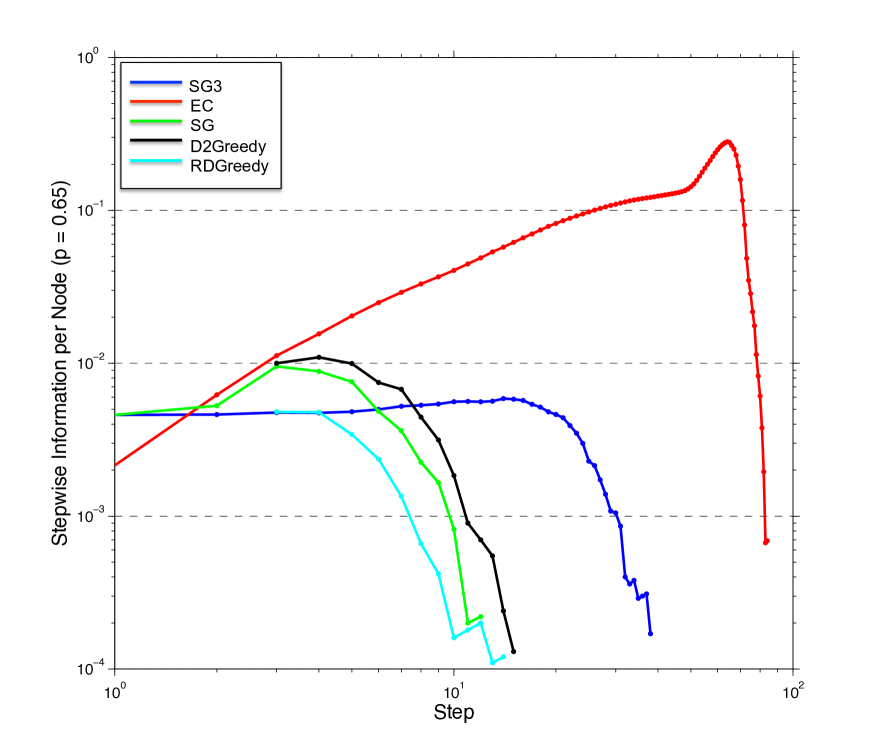
(a) Edge Reversal Model, $n$: 100, $p=0.65$

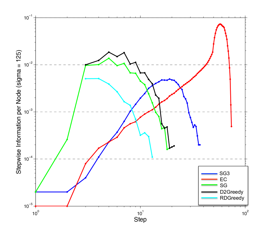
(b) Gaussian Edge Weights Model, $n$: 100, $\sigma=125$

Figure 2: Stepwise Information per Node

The information content is computed as the maximum stepwise information $I^{\mathscr{A}}:=\max_{t}I_{t}^{\mathscr{A}}$. Notice that $\log\Delta_{t}^{\mathscr{A}}(G^{\prime},G^{\prime\prime})$ measures the ability of $\mathscr{A}$ to find common solutions for the two noisy instances $G^{\prime},G^{\prime\prime}$, given the underlying input graph $G$.

Our results support the following observations and analysis:

$\bullet$ All investigated algorithms reach the maximum information content in the noise free limit ($G^{\prime}=G^{\prime\prime}$), i.e., for $p=0,1$ in the edge reversal model and for $\sigma=0$ in the Gaussian edge weights model. In this circumstance, $\mathbb{E}\log\Delta_{t}^{\mathscr{A}}(G^{\prime},G^{\prime\prime})=\log|C_{t}^{\mathscr{A}}(G^{\prime})|=n-t-1$, so $I_{t}^{\mathscr{A}}=t+\log(2^{n-1}-1)-(n-1)$, and the information content reaches its maximum $\log(2^{n-1}-1)$ at the final step $t=n-1$.

$\bullet$ Fig. 1(a) demonstrates that the information content qualitatively agrees with the consistency between two noisy instances (the dashed magenta line), which reflects that $\log\Delta_{t}^{\mathscr{A}}(G^{\prime},G^{\prime\prime})$ is affected by the noisy instances.

$\bullet$ Stepwise information (Fig.  2) of the algorithms increase initially, but after reaching the optimal step $t^{*}$ (the step with highest information), it decreases and finally vanishes.

$\bullet$ For the greedy heuristics, backward greedy is more informative than double greedy under both models. EC (backward greedy) achieves the highest information content. We explain this behavior by delayed decision making of the backward greedy edge contraction. With high probability it preserves consistent solutions by contracting low weight edges that have a low probability to be included in the cut. The same phenomena arises for the reverse-delete algorithm to calculate the minimum spanning tree of a graph (see [13]).

$\bullet$ The information content of the four double greedy algorithms achieve different rank orders for the two models. SG3 is inferior to other double greedy algorithms under Gaussian edge weights model, but this only happens when $p\in[0.2,0.87]$ for the edge reversal model. This results from that information content of one specific algorithm is affected by both the input master graph $G$ and the noisy instances $G^{\prime},G^{\prime\prime}$, which are completely different under the two models.

$\bullet$ Different greedy techniques cast different influences on the information content. The four double greedy algorithms differ by the techniques they use (Table  I). (1) The randomization technique makes RDGreedy very fragile w.r.t. information content, though it improves the worst-case approximation guarantee for the general USM problem ([14]). RDGreedy labels each vertex with a probability proportional to the objective gain, this randomization makes the consistency between $|C_{t}^{\mathscr{A}}(G^{\prime})|$ and $|C_{t}^{\mathscr{A}}(G^{\prime\prime})|$ very weak, resulting in small approximation set intersection $\log\Delta_{t}^{\mathscr{A}}(G^{\prime},G^{\prime\prime})$. (2) The initializing strategy for the first 2 vertices as used in SG decreases the information content (SG is outperformed by D2Greedy under both models) due to early decision making. (3) The situation is similar for the sorting techniquey used in SG3 under Gaussian edge weights model, it is outperformed by both SG and D2Greedy. But for the edge reversal model, this observation only holds when $p\in[0.2,0.87]$.

$\bullet$ SG and D2Greedy behave very similar under both models, which is caused by an equivalent processing sequence apart from initializing of the first two vertices (proved in Supplement VI-B).

V Discussion and Conclusion

This work advocates an information theoretically guided average case analysis of the generalization ability of greedy MaxCut algorithms. We have contributed to the foundation of approximation set coding by presenting provably correct methods to exactly compute the cardinality of approximation sets. The counting algorithms for approximate solutions enable us to explore the information content of greedy MaxCut algorithms. Based on the observations and analysis, we propose the following conjecture:

$\bullet$ Different greedy heuristics (backward, double) and different processing techniques (sorting, randomization, intilization) sensitively influence the information content. The backward greedy with its delayed decision making consistently outperforms the double greedy strategies for different noise models and noise levels.

Since EC demonstrated to achieve the highest robustness, it is valuable to develop the corresponding algorithm for the general USM.

In this work ASC has been employed as a descriptive tool to compare algorithms. We could also use the method for algorithm design. A meta-algorithm modifies the algorithmic steps of a MaxCut procedure and measures the resulting change in information content. Beneficial changes are accepted and detrimental changes are rejected. It is also imaginable that design principles like delayed decision making are systematically identified and then combined to improve the informativeness of novel algorithms.

VI Supplementary Material

VI-A Details of Double Greedy Algorithms

Input: A complete graph $G=(V,E)$ with nonnegative edge weights $w_{ij},\forall i,j\in V,i\neq j$

Output: A disjoint cut and the cut value

1 Pick the maximum weighted edge $(x,y)$;

2 $S_{1}:=\{x\}$,$S_{2}:=\{y\}$, $cut(S_{1},S_{2}):=w_{xy}$;

3 for $i=1:n-2$ do

       If $w(i,S_{1})>w(i,S_{2})$, then add $i$ to $S_{2}$, else add it to $S_{1}$;

        // $w(i,S_{k}):=\sum_{j\in S_{k}}w_{ij},k=1,2$

4       $cut(S_{1},S_{2}):=cut(S_{1},S_{2})+\max\{w(i,S_{1}),w(i,S_{2})\}$;

5      

return $S_{1}$, $S_{2}$, and $cut(S_{1},S_{2})$

Algorithm 4 SG ([15])

Input: A complete graph $G=(V,E)$ with nonnegative edge weights $w_{ij},\forall i,j\in V,i\neq j$

Output: A disjoint cut and the cut value

1 $S^{0}:=\emptyset$, $T^{0}:=V$;

2 for $i=1$ to $n$ do

3       $a_{i}:=f(S^{i-1}\cup\{v_{i}\})-f(S^{i-1})$;

4       $b_{i}:=f(T^{i-1}\backslash\{v_{i}\})-f(T^{i-1})$;

5       $a_{i}^{\prime}:=\max\{a_{i},0\}$, $b_{i}^{\prime}:=\max\{b_{i},0\}$;

       With probability $\frac{a_{i}^{\prime}}{a_{i}^{\prime}+b_{i}^{\prime}}$ do: $S^{i}:=S^{i-1}\cup\{v_{i}\}$, $T^{i}:=T^{i-1}$ // If $a_{i}^{\prime}=b_{i}^{\prime}=0$, assume $\frac{a_{i}^{\prime}}{a_{i}^{\prime}+b_{i}^{\prime}}=1$

6       Else (with the compliment probability $\frac{b_{i}^{\prime}}{a_{i}^{\prime}+b_{i}^{\prime}}$) do: $S^{i}:=S^{i-1}$, $T^{i}:=T^{i-1}\backslash\{v_{i}\}$;

7      

return 2 subsets: $S^{n}$, $V\backslash S^{n}$, and $cut(S^{n},V\backslash S^{n})$

Algorithm 5 RDGreedy ([14])

Input: A complete graph $G=(V,E)$ with nonnegative edge weights $w_{ij},\forall i,j\in V,i\neq j$

Output: A disjoint cut $S_{1},S_{2}$ and the cut value $cut(S_{1},S_{2})$

1 Pick the maximum weighted edge $(x,y)$;

2 $S_{1}:=\{x\}$,$S_{2}:=\{y\}$,$V:=V\backslash\{x,y\}$, $cut(S_{1},S_{2}):=w_{xy}$;

3 for $i=1:n-2$ do

4       for $j\in V$ do

             $score(j):=|w(j,S_{1})-w(j,S_{2})|$ ;

              // $w(j,S_{k}):=\sum_{j^{\prime}\in S_{k}}w_{jj^{\prime}},k=1,2$

5            

6      Choose the vertex $j^{*}$ with the maximum score;

7       If $w(j^{*},S_{1})>w(j^{*},S_{2})$, then add $j^{*}$ to $S_{2}$, else add it to $S_{1}$;

8       $V:=V\backslash\{j^{*}\}$;

9       $cut(S_{1},S_{2}):=cut(S_{1},S_{2})+\max\{w(j^{*},S_{1}),w(j^{*},S_{2})\}$;

10      

return $S_{1}$, $S_{2}$, and $cut(S_{1},S_{2})$

Algorithm 6 SG3

VI-B Equivalence Between Labelling Criterions of SG and D2Greedy

Claim:  Except for processing the first 2 vertices, D2Greedy and SG conduct the same labelling strategy for each vertices.

Proof.

To verify this, assume in the beginning of a certain step $i$, the solution set pair of SG is $(S_{1},S_{2})$, of D2Greedy is $(S,T)$ (for simplicity omit the step index here).

Note that the relationship between solution sets of SG and D2Greedy is: $S_{1}\leftrightarrow S$ and $S_{2}\leftrightarrow(V\backslash T)$.

For SG, the labelling criterion for vertex $i$ is:

$$w(i,S_{2})-w(i,S_{1})=\sum_{i,j\in S_{2}}w_{ij}-\sum_{i,j\in S_{1}}w_{ij}$$ (4)

For D2Greedy, the labelling criterion for vertex $i$ is:

$$a_{i}-b_{i} =[f(S\cup\{v_{i}\})-f(S)]-[f(T\backslash\{v_{i}\})-f(T)]$$

$$=\left(\sum_{i\in S\cup\{v_{i}\},j\in V\backslash S\backslash\{v_{i}\}}w_{ij}-\sum_{i\in S,j\in V\backslash S}w_{ij}\right)-$$

$${\phantom{=}}\left(\sum_{i\in T\backslash\{v_{i}\},j\in V\backslash T\cup\{v_{i}\}}w_{ij}-\sum_{i\in T,j\in V\backslash T}w_{ij}\right)$$ (5)

$$=\left(\sum_{i,j\in V\backslash S\backslash\{v_{i}\}}w_{ij}-\sum_{i\in S,j=i}w_{ij}\right)-$$

$${\phantom{=}}\left(\sum_{i\in T\backslash\{v_{i}\},j=i}w_{ij}-\sum_{i,j\in V\backslash T}w_{ij}\right)$$ (6)

$$=\left(\sum_{i,j\in(V\backslash T)\cup(T\backslash S\backslash\{v_{i}\})}w_{ij}-\sum_{i,j\in S}w_{ij}\right)-$$

$${\phantom{=}}\left(\sum_{i,j\in(S)\cup(T\backslash S\backslash\{v_{i}\})}w_{ij}-\sum_{i,j\in V\backslash T}w_{ij}\right)$$ (7)

$$=2\left(\sum_{i,j\in V\backslash T}w_{ij}-\sum_{i,j\in S}w_{ij}\right)$$

$$=2\left(\sum_{i,j\in S_{2}}w_{ij}-\sum_{i,j\in S_{1}}w_{ij}\right)$$ (8)

$$=2[w(i,S_{2})-w(i,S_{1})]$$

where Eq. 8 comes from the relationship between solution sets of SG and D2Greedy.

So the labelling criterion for SG and D2Greedy is equivalent with each other. ∎

VI-C Counting Methods for Double Greedy Algorithms

D2Greedy: summarized in Alg. 1, we have proved that it has the same labelling criterion with SG, the relationship between solution sets of SG and D2Greedy is: $S_{1}\leftrightarrow S$ and $S_{2}\leftrightarrow(V\backslash T)$, we will use $S_{1}$ and $S_{2}$ in the description of its counting methods.

In step $t$ ($t=1,\cdots,n$) there are $k=n-t$ unlabelled vertices, it is not difficult to know that the number of possible solutions for each instance is

$$|C(G^{\prime})|=|C(G^{\prime\prime})|=\left\{\begin{array}[]{ll}2^{k}&\textrm{if $S_{1}\neq\emptyset$ and $S_{2}\neq\emptyset$}\\ 2^{k}-1&\textrm{otherwise}\\ \end{array}\right.$$

To count the intersection set (i.e. $|C(G^{\prime})\cap C(G^{\prime\prime})|$), assume the solution sets of $G^{\prime}$ is $(S_{1}^{\prime},S_{2}^{\prime})$, the solution sets of $G^{\prime\prime}$ is $(S_{1}^{\prime\prime},S_{2}^{\prime\prime})$, so the unlabelled vertex sets are $T^{\prime}=V\backslash S_{1}^{\prime}\backslash S_{2}^{\prime}$, $T^{\prime\prime}=V\backslash S_{1}^{\prime\prime}\backslash S_{2}^{\prime\prime}$, respectively. Denote $L:=T^{\prime}\cap T^{\prime\prime}$ be the common vertices of the two unlabelled vertex sets, so $l=|L|$ ($0\leq l\leq k$) is the number of common vertices in the unlabelled $k$ vertices. Denote $M^{\prime}:=T^{\prime}\backslash L$, $M^{\prime\prime}:=T^{\prime\prime}\backslash L$ be the sets of different vertex sets between the two unlabelled vertex sets. Then,

1. if $(S_{1}^{\prime}\backslash M^{\prime\prime},S_{2}^{\prime}\backslash M^{\prime\prime})$ or $(S_{2}^{\prime}\backslash M^{\prime\prime},S_{1}^{\prime}\backslash M^{\prime\prime})$ matches $(S_{1}^{\prime\prime}\backslash M^{\prime},S_{2}^{\prime\prime}\backslash M^{\prime})$.

   Assume w.l.o.g. that $(S_{1}^{\prime}\backslash M^{\prime\prime},S_{2}^{\prime}\backslash M^{\prime\prime})$ matches $(S_{1}^{\prime\prime}\backslash M^{\prime},S_{2}^{\prime\prime}\backslash M^{\prime})$:

   $$\begin{split}&|C(G^{{}^{\prime}})\cap C(G^{{}^{\prime\prime}})|=\\ &\left\{\begin{array}[]{ll}2^{l}&\textrm{if $S_{1}^{\prime}\cup S_{1}^{\prime\prime}\neq\emptyset$ and $S_{2}^{\prime}\cup S_{2}^{\prime\prime}\neq\emptyset$}\\ 2^{l}-1&\textrm{otherwise}\\ \end{array}\right.\end{split}$$

2. otherwise, $|C(G^{{}^{\prime}})\cap C(G^{{}^{\prime\prime}})|$ = 0

SG3: presented in Section III-A.

SG: summarized in Alg. 4, the methods to count its approximation sets is the same as that of SG3.

RDGreedy: summarized in Alg. 5, the methods to count its approximation sets is the same as that of D2Greedy.

VI-D Proof of the Correctness of Method to Count $|C(G^{\prime})\cap C(G^{\prime\prime})|$ of SG3

Proof.

First of all, notice that $M^{\prime}$ must be included in $S_{1}^{\prime\prime}\cup S_{2}^{\prime\prime}$ and $M^{\prime\prime}$ must be included in $S_{1}^{\prime}\cup S_{2}^{\prime}$, because $M^{\prime}$ has no intersection with $M^{\prime\prime}$, and we know that $S_{1}^{\prime\prime}\cup S_{2}^{\prime\prime}\cup M^{\prime\prime}=S_{1}^{\prime}\cup S_{2}^{\prime}\cup M^{\prime}$. After removing $M^{\prime}$ from $S_{1}^{\prime\prime}\cup S_{2}^{\prime\prime}$, and $M^{\prime\prime}$ from $S_{1}^{\prime}\cup S_{2}^{\prime}$, the vertices in the pairs, $(S_{1}^{\prime}\backslash M^{\prime\prime},S_{2}^{\prime}\backslash M^{\prime\prime})$ and $(S_{1}^{\prime\prime}\backslash M^{\prime},S_{2}^{\prime\prime}\backslash M^{\prime})$, can not be changed by distributing any other unlabelled vertices , so if they can not match with each other, there will be no common solutions.

If they can match, in the following, there is only one way to distribute $M^{\prime}$ and $M^{\prime\prime}$ to have common solutions. And the vertices in the common set $L=T^{\prime}\cap T^{\prime\prime}$ can be distributed consistently in the two instances, so in this situation $|C(G^{\prime})\cap C(G^{\prime\prime})|=2^{l}$. ∎

VI-E Proof of Theorem 1

Proof.

First of all, We will prove the following claim, then use the claim to prove Theorem 1.

Claim:  In each step $t$ ($t=0,\cdots,n-2$), the following conditions hold:

1. The remained super vertices in $P,Q$ are distinct with each other, that means any 2 super vertices inside $P$ or $Q$ do not have intersection, and there are no common super vertex between $P$ and $Q$.

2. The common super vertex removed from $P,Q$, i.e., $\mathbf{p_{ii^{\prime}}}=\mathbf{q_{jj^{\prime}}}$, is the smallest common super vertex containing $\mathbf{p}_{i}$ or $\mathbf{p}_{i^{\prime}}$ (respectively, $\mathbf{q}_{j}$ or $\mathbf{q}_{j^{\prime}}$)

3. The common super vertex removed from $P,Q$, i.e., $\mathbf{p_{ii^{\prime}}}=\mathbf{q_{jj^{\prime}}}$, are “unique” (i.e., there does not exist $\mathbf{p_{ii^{\prime\prime}}}=\mathbf{q_{jj^{\prime\prime}}}$, such that $\mathbf{p_{ii^{\prime\prime}}}\neq\mathbf{p_{ii^{\prime}}}$). That means, there is only one possible way to construct the removed common super vertex.

We will use inductive assumption to prove the claim. First of all, in the beginning (step 0), the conditions hold. Assume the conditions hold in step $t$. In step $t+1$, there are 2 possible situations:

• There are no common super vertex removed.

  Condition 1 holds because the contracted super vertices pair do not equal. Condition 2, 3 hold as well because there are no contracted super vertices removed.

• There are common super vertex removed.

  Condition 1 holds because the only common super vertices pair have been removed from $P,Q$, respectively.
  

  To prove condition 2, notice that the smaller vertices for $\mathbf{p_{ii^{\prime}}}$ are $\mathbf{p_{ii^{\prime}}}\backslash\mathbf{p_{i}}=\mathbf{p_{i^{\prime}}}$ and $\mathbf{p_{ii^{\prime}}}\backslash\mathbf{p_{i}^{\prime}}=\mathbf{p_{i}}$, respectively, for $\mathbf{q_{jj^{\prime}}}$ are $\mathbf{q_{jj^{\prime}}}\backslash\mathbf{q_{j}}=\mathbf{q_{j^{\prime}}}$ and $\mathbf{q_{jj^{\prime}}}\backslash\mathbf{q_{j}^{\prime}}=\mathbf{q_{j}}$, according to Condition 1, they can not be common super vertices, so there are no smaller common super vertices.
  

  To prove condition 3, assume there exists $\mathbf{p_{ii^{\prime\prime}}}=\mathbf{q_{jj^{\prime\prime}}}$, such that $\mathbf{p_{ii^{\prime\prime}}}\neq\mathbf{p_{ii^{\prime}}}$ (respectively, $\mathbf{q_{jj^{\prime\prime}}}\neq\mathbf{q_{jj^{\prime}}}$), so $\mathbf{p_{i^{\prime\prime}}}\neq\mathbf{p_{i^{\prime}}}$ ($\mathbf{p_{j^{\prime\prime}}}\neq\mathbf{p_{j^{\prime}}}$). From Alg. 3 we know that $\mathbf{p_{i}}\cup\mathbf{p_{i^{\prime\prime}}}=\mathbf{p_{ii^{\prime\prime}}}\supseteq\mathbf{q_{j}}\backslash\mathbf{p_{i}}$ and $\mathbf{p_{i}}\cup\mathbf{p_{i^{\prime}}}=\mathbf{p_{ii^{\prime}}}\supseteq\mathbf{q_{j}}\backslash\mathbf{p_{i}}$ (respectively, $\mathbf{q_{j}}\cup\mathbf{q_{j^{\prime\prime}}}=\mathbf{q_{jj^{\prime\prime}}}\supseteq\mathbf{p_{i}}\backslash\mathbf{q_{j}}$ and $\mathbf{q_{j}}\cup\mathbf{q_{j^{\prime}}}=\mathbf{q_{jj^{\prime}}}\supseteq\mathbf{p_{i}}\backslash\mathbf{q_{j}}$), so that $\mathbf{p_{i^{\prime\prime}}}\supseteq\mathbf{q_{j}}\backslash\mathbf{p_{i}}$ and $\mathbf{p_{i^{\prime}}}\supseteq\mathbf{q_{j}}\backslash\mathbf{p_{i}}$ (respectively, $\mathbf{q_{j^{\prime\prime}}}\supseteq\mathbf{p_{i}}\backslash\mathbf{q_{j}}$ and $\mathbf{q_{j^{\prime}}}\supseteq\mathbf{p_{i}}\backslash\mathbf{q_{j}}$), that contradicts the known truth that $\mathbf{p_{i^{\prime}}}$ and $\mathbf{p_{i^{\prime\prime}}}$ (respectively, $\mathbf{q_{j^{\prime}}}$ and $\mathbf{q_{j^{\prime\prime}}}$) must be totally different with each other (from Condition 1).

Then we use the Claim to prove that the $c$ returned by Alg. 3 is exactly the maximum number of common super vertices after all possible contractions. Because the 3 conditions hold for each step, we know that finally all the common super vertices are removed out from $P$ and $Q$. From Condition 2 we know that all the removed common super vertices are the smallest ones, from Condition 3 we get that there is not a second way to construct the common super vertices, so the resulted $c$ is the maximum number of common super vertices after all possible contractions.

∎

References

• [1] J. Wang, T. Jebara, and S.-F. Chang, “Semi-supervised learning using greedy max-cut,” JMLR, vol. 14, no. 1, pp. 771–800, Mar. 2013.
• [2] R. Agrawal, S. Rajagopalan, R. Srikant, and Y. Xu, “Mining newsgroups using networks arising from social behavior,” in WWW.   ACM, 2003, pp. 529–535.
• [3] F. Barahona, M. Grötschel, M. Jünger, and G. Reinelt, “An application of combinatorial optimization to statistical physics and circuit layout design,” Operations Research, vol. 36, no. 3, pp. 493–513, 1988.
• [4] E. Halperin and U. Zwick, “Combinatorial approximation algorithms for the maximum directed cut problem,” in ACM-SIAM symposium on Discrete algorithms, 2001, pp. 1–7.
• [5] A. A. Ageev and M. Sviridenko, “An 0.828-approximation algorithm for the uncapacitated facility location problem,” Discrete Applied Mathematics, vol. 93, no. 2, pp. 149–156, 1999.
• [6] G. Cornuejols, M. Fisher, and G. L. Nemhauser, “On the uncapacitated location problem,” Annals Discr. Math., vol. 1, pp. 163–177, 1977.
• [7] J. M. Buhmann, “Information theoretic model validation for clustering.” in ISIT, 2010, pp. 1398–1402.
• [8] J. Buhmann, “Context sensitive information: Model validation by information theory,” in Pattern Recognition, ser. LNCS 6718.   Springer Berlin / Heidelberg, 2011, pp. 12–21.
• [9] J. M. Buhmann, “Simbad: Emergence of pattern similarity,” in Similarity-Based Pattern Analysis and Recognition.   Springer, 2013, pp. 45–64.
• [10] M. H. Chehreghani, A. G. Busetto, and J. M. Buhmann, “Information theoretic model validation for spectral clustering.” in AISTATS, 2012, pp. 495–503.
• [11] G. Zhou, S. Geman, and J. M. Buhmann, “Sparse feature selection by information theory,” in ISIT.   IEEE, 2014, pp. 926–930.
• [12] L. M. Busse, M. H. Chehreghani, and J. M. Buhmann, “The information content in sorting algorithms,” in ISIT.   IEEE, 2012, pp. 2746–2750.
• [13] A. Gronskiy and J. M. Buhmann, “How informative are minimum spanning tree algorithms?” in ISIT.   IEEE, 2014, pp. 2277 – 2281.
• [14] N. Buchbinder, M. Feldman, J. Naor, and R. Schwartz, “A tight linear time (1/2)-approximation for unconstrained submodular maximization,” in FOCS.   IEEE, 2012, pp. 649–658.
• [15] S. Sahni and T. Gonzalez, “P-complete approximation problems,” Journal of the ACM (JACM), vol. 23, no. 3, pp. 555–565, 1976.
• [16] S. Kahruman, E. Kolotoglu, S. Butenko, and I. V. Hicks, “On greedy construction heuristics for the max-cut problem,” Int. J. Comput. Science and Engineering, vol. 3, no. 3, pp. 211–218, 2007.