Waves on accelerating dodecahedral universes

Abstract.

We investigate the wave propagation on a compact $3$-manifold of constant positive curvature with a non trivial topology, the Poincaré dodecahedral space, if the scale factor is exponentially increasing. We prove the existence of a limit state as $t\rightarrow+\infty$ and we get its analytic expression. The deep sky is described by this asymptotic profile thanks to the Sachs-Wolfe formula. We transform the Cauchy problem into a mixed problem posed on a fundamental domain determined by the quaternionic calculus. We perform an accurate scheme of computation: we employ a variational method using a space of second order finite elements that is invariant under the action of the binary icosahedral group.

I. Introduction

The topology and the geometry of our universe is a fundamental open problem. There are a lot of articles about these topics (for example [23, 24, 35]). Recently the data by WMAP (Wilkinson Microwave Anisotropy Probe) mission have provided strong evidence suggesting that the observable universe is nearly flat, with the ratio of its total matter-energy density to the critical value very close to one [7], but without fixing the sign of its curvature. So the study of the wave propagation in universes involving the Poincaré dodecahedral space continues to be relevant in particular for the search of the circles-in-the-sky signature [1], [2], [27]. This model has received a lot of interest and generated numerous works (see e.g. [1, 5, 8, 20, 25, 30, 36]). These spacetimes are Lorentzian manifolds $({\mathbb{R}}_{t}\times\mathbf{K},g)$ that are globally hyperbolic and multi-connected. Here $\mathbf{K}$ is the Poincaré dodecahedral space that is a three dimensional $C^{\infty}$ compact manifold, without boundary, defined as the quotient of the 3-sphere $\mathcal{S}^{3}$ under the action of the binary icosahedral group $\mathcal{I}^{*}$ ([14, 31, 34, 37]). In [5] we have investigated the propagation of the scalar waves in the case of the stationary universe for which $ds^{2}=dt^{2}-ds^{2}_{\mathbf{K}}$ where $ds^{2}_{\mathbf{K}}$ is the Euclidean metric induced by the three-sphere $\mathcal{S}^{3}$ on $\mathbf{K}$. In this paper we study the wave propagation on dynamical universes $(\mathcal{U},g)$ of Robertson-Walker type

(I.1) $$\mathcal{U}={\mathbb{R}}_{t}\times\mathbf{K},\;\;ds_{\mathcal{U}}^{2}=g_{\mu\nu}dx^{\mu}dx^{\nu}=dt^{2}-a^{2}(t)ds^{2}_{\mathbf{K}},$$

where the scale factor $a(t)$ is a smooth positive function. We are mainly interested in considering the accelerating spacetimes for which the scale factor is an increasing function with an exponential behaviour, $a(t)\sim e^{\alpha t}$ as $t\rightarrow\infty$. In the study of the asymptotics of the fields at the infinity, and for the numerical experiments, we treat two important cases. In the first one, we choose $a(t)=H^{-1}\cosh(Ht)$ where $H>0$ is the Hubble constant. Then $g$ is solution of the vacuum Einstein equations with cosmological constant $\Lambda=3H^{2}$ and $\mathcal{U}$ is locally isometric to the de Sitter spacetime $d\mathcal{S}_{4}$ and differs globally from $d\mathcal{S}_{4}$ by its topology that is not trivial. We denote this universe $d\mathcal{S}_{4}\left(\mathbf{K}\right)$. In particular, while $d\mathcal{S}_{4}$ is spatially homogeneous and globally isotropic, $d\mathcal{S}_{4}(\mathbf{K})$ is homogeneous but not globally isotropic [26]. In the second model we choose $a(t)=e^{t}$. Then $g$ is no longer a solution of the vacuum Einstein equations but it is a toy model for a universe with an inflation generated by a scalar field or a solution in $f(T)$ theory (see e.g. [16]).

In this paper we investigate the scalar waves on $(\mathcal{U},g)$ that are the solutions of the D’Alembert equation

$${\Box}_{g}\Psi:=\frac{1}{\sqrt{|g|}}\partial_{\mu}\left(g^{\mu\nu}\sqrt{|g|}\partial_{\nu}\Psi\right)=0.$$

For the spacetime (I.1), this equation has the form

(I.2) $$\left[\partial_{t}^{2}+3\frac{a^{\prime}(t)}{a(t)}\partial_{t}-\frac{1}{a^{2}(t)}\Delta_{\mathbf{K}}\right]\Psi=0,$$

where $\Delta_{\mathbf{K}}$ is the Laplace-Beltrami operator on $\mathbf{K}$. This equation plays a fundamental role in the theory of cosmological perturbations (see e.g. [28]). It arises in the linearized Einstein equations in the vacuum, written in harmonic coordinates, and in this case $\Psi$ is the fluctuation around the ground metric, i.e. $\Psi$ describes the gravitational waves. On the other hand the Sachs-Wolfe theorem assures that in the Friedmann-Robertson-Walker universe with an ultrarelativistic gas, the scalar perturbations obey to this acoustic equation. This result was proved originally for the spatially flat metric, and has been extended to arbitrary space curvature [12], [15]. In this context, considered in [1], [2], we write the ground metric (I.1) as

$$ds^{2}_{\mathcal{U}}=A(\eta)\left[d\eta^{2}-ds_{\mathbf{K}}^{2}\right],\;\;ds^{2}_{\mathbf{K}}=d\chi^{2}+\sin^{2}\chi\left(d\theta^{2}+\sin^{2}\theta d\varphi^{2}\right),$$

where $\eta=\int a^{-1}(t)dt$ is the conformal time, and $A(\eta)=a(t)$ is the cosmic scale factor. Then, the metric with the scalar perturbation $\Psi$ takes the form in conformal Newtonian gauge:

(I.3) $$ds^{2}=A(\eta)\left[(1+2\Psi)d\eta^{2}-(1-2\Psi)ds_{\mathbf{K}}^{2}\right].$$

The knowledge of $\Psi$ allows to adress a fundamental issue of the cosmology: the study of the temperature fluctuations $\delta T(\theta,\varphi)$ of the temperature $T(\theta,\varphi)$ of the cosmic microwave background radiation, observed in the direction $(\theta,\varphi)\in S^{2}$. The integrated Sachs-Wolfe formula (see i.e. [1]) gives a link between $\delta T/T$ observed at the conformal time $\eta_{0}$ of our present epoch, and $\Psi$ between $\eta_{0}$ and $\eta_{ls}$, the conformal time at recombination ([1], formula (31)). Therefore we must know the time evolution of $\Psi$ to be able to use it. An approximated formula for low spherical harmonics is also given by the ordinary Sachs-Wolfe formula,

(I.4) $$\frac{\delta T(\theta,\varphi)}{T}\simeq\frac{1}{3}\Psi(\eta_{ls},\chi=\eta_{0}-\eta_{ls},\theta,\varphi).$$

If $\eta_{0}-\eta_{ls}>\arccos\left(\frac{\sigma^{2}}{2\sqrt{2}}\right)$ where $\sigma$ is the golden ratio, the horizon radius of the observer is larger than the injectivity radius, hence repeating images of the sphere horizon intersect each other. Since the self-intersections of the sphere of last scattering are circles, the fluctuations of a realistic $\Psi(\eta_{ls},\chi=\eta_{0}-\eta_{ls},.)$, for instance if the primordial fluctuation amplitude $\Psi(0,.)$ is a Gaussian random variable, would be correlated around circles: the observer can see circles-in-the-sky [11].

Besides, we remark that, as regards the propagation of the electromagnetic fields in the curved space-times, the D’Alembert operator ${\Box}_{g}=\nabla^{\alpha}\partial_{\alpha}$ is also the principal part of the Maxwell equation for the vector potential $\nabla^{\alpha}\nabla_{\alpha}A^{\beta}-R^{\beta}_{\lambda}A^{\lambda}=J^{\beta}$. In concluding, there are numerous motivations to study this equation, represent and compute the solutions, investigate their properties.

The explicit form of the solutions is known for the classic F-R-W space-time with the ${\mathbb{R}}\times S^{3}$ topology [19]. The case of the dodecahedral space is much more complicated. In this work we solve the Cauchy problem, we represent the solutions in terms of expansions involving the eigenmodes of the Laplacian on $\mathbf{K}$, then we investigate the asymptotic behaviour of $\Psi$ at the time infinity, and finally we develop a numerical scheme of accurate computation. A crucial result is the exponentially fast convergence of $\Psi(t,X)$ to a final asymptotic state $\Psi_{\infty}(X)$ when $t$ tends to the infinity. The link between $\Psi_{\infty}$ and the initial data of $\Psi$ is given by a pseudodifferential operator. In particular for $d\mathcal{S}_{4}\left(\mathbf{K}\right)$, we have

(I.5) $$\Psi_{\infty}=\left(-\Delta_{\mathbf{K}}+1\right)^{-\frac{1}{2}}\sin\left(\frac{\pi}{2}\sqrt{-\Delta_{\mathbf{K}}+1}\right)\Psi(0,.)+\frac{\sqrt{15}}{4}\int_{\mathbf{K}}\partial_{t}\Psi(0,.)\omega_{\mathbf{K}},$$

where $\omega_{\mathbf{K}}$ is the volume form on $\mathbf{K}$. To compute $\Psi_{\infty}$ with this formula we should use the eigenfunctions of the Laplacian. Despite significant progress for the determination of these modes (see in particular [6], [20]), the implementation of this strategy seems to be challenging. Instead, we solve numerically the initial value problem, and taking advantage of the fast convergence, we simply find the asymptotic profile as

$$\Psi_{\infty}(X)=\lim_{t\rightarrow+\infty}\Psi(t,X)\sim\Psi(T,X),\;\;T>>1.$$

From the point of view of the theory of cosmological perturbations, this result has a great interest if $\Psi$ is the scalar perturbation in the metric (I.3). If the conformal time of recombination is large enough, we have $\Psi(\eta_{ls},.)\simeq\Psi_{\infty}$. Then the approximated Sachs-Wolfe formula becomes

(I.6) $$\frac{\delta T(\theta,\varphi)}{T}\simeq\frac{1}{3}\Psi_{\infty}(\chi=\eta_{0}-\eta_{ls},\theta,\varphi),$$

and the circles-in-the-sky have simply to be found in $\Psi_{\infty}$.

We briefly describe the following sections. In part 2 we solve the global Cauchy problem for (I.2) in the functional framework associated to the energy

(I.7) $$E(\Psi,t):=\|\partial_{t}\Psi(t)\|^{2}_{L^{2}(\mathbf{K})}+\frac{1}{a^{2}(t)}\|\nabla_{\mathbf{K}}\Psi(t)\|^{2}_{L^{2}(\mathbf{K})}.$$

We represent the Poincaré dodecahedral space by its fundamental domain $\mathcal{F}$ that is the geodesic convex hull of twenty vertices on $\mathcal{S}^{3}$ that are included in $\{x_{0}=\frac{\sigma^{2}}{2\sqrt{2}}\}\times{\mathbb{R}}^{3}$ where $\sigma$ is the golden ratio. We introduce the domain of vizualisation $\mathcal{F}_{v}\subset{\mathbb{R}}^{3}$ that is the projection $(x_{0},x_{1},x_{2},x_{3})\in\mathcal{S}^{3}\mapsto(x_{1},x_{2},x_{3})\in{\mathbb{R}}^{3}$ of the fundamental domain. $\mathcal{F}_{v}$ is a dodecahedron with pentagonal curved faces included in ellipsoids (figure(1)). Defining $u(t,x_{1},x_{2},x_{3}):=\Psi(t,x_{0},x_{1},x_{2},x_{3})$ the wave equation (I.2) is equivalent to

(I.8) $$\left[\partial_{t}^{2}+3\frac{a^{\prime}(t)}{a(t)}\partial_{t}-\frac{1}{a^{2}(t)}\Delta_{\mathcal{F}_{v}}\right]u=0,\;\;t\in{\mathbb{R}},\;\;x\in\mathcal{F}_{v},$$

together with the boundaries conditions

(I.9) $$\forall\tau\in\mathcal{I}^{*},\;(x^{\prime}_{0},x^{\prime}_{1},x^{\prime}_{2},x^{\prime}_{3})=\tau(x_{0},x_{1},x_{2},x_{3})\Rightarrow u(t,x^{\prime}_{1},x^{\prime}_{2},x^{\prime}_{3})=u(t,x_{1},x_{2},x_{3}).$$

We solve the initial value problem associated to (I.8) and (I.9) and we state an equivalent variational problem. We discuss the existence of a future horizon and we compute the radius of the horizon sphere.

In the third section we investigate the asymptotic behaviour of $\Psi(t,.)$ as $t\rightarrow+\infty$. We prove the existence of an asymptotic profile $\Psi_{\infty}:=\lim_{t\rightarrow\infty}\Psi(t)$ if the scale factor is exponentially increasing, and we compute an analytic expression of $\Psi_{\infty}$ in the cases $a(t)=H^{-1}\cosh(Ht)$ and $a(t)=e^{t}$. These results extend those of [3] regarding the steady state universe (see also [33]). We estimate the norms of $\Psi_{\infty}$ by the energy of $\Psi$.

In the fourth part we numerically investigate the mixed problem (I.8, I.9). We are mainly interested in computing the waves for a long time, hence the exponential behaviour of the coefficients in the equation leads to a hard numerical challenge. To overcome this difficulty we have to perform very precise computations. To reach this goal we adopt the variational method associated to (I.8) with suitable finite elements satisfying constraint (I.9). In the case of the stationary universes we used in [5] finite elements of ${\mathbb{P}}_{1}$ type. To be able to treat the accelerating universes, we need more precision and we use elements of second order. Our numerical results are in excellent agreement with the theoretical results on the radius of the future horizon and on the asymptotic behaviours of the waves.

II. Waves on dynamical universes

In this section we solve the global Cauchy problem for the D’Alembert equation on the dynamical universes (I.1). We assume the scale factor $a$ is a $C^{\infty}$ function that is strictly positive. As a direct consequence of the theorem of Choquet-Bruhat, Cotsakis (Theorem 11.10 of [9]), we can see that $(\mathcal{U},g)$ is a globally hyperbolic manifold. Therefore according to Leray [22], the global Cauchy problem is well posed in $C^{\infty}$. Now it is natural to look for the solutions in the scale of the Hilbert spaces associated to the energy (I.7). Given $m\in{\mathbb{N}}$, we introduce the Sobolev space

$$H^{m}(\mathbf{K}):=\left\{\Psi\in L^{2}(\mathbf{K}),\;\nabla_{\mathbf{K}}^{\alpha}\Psi\in L^{2}(\mathbf{K}),\;\mid\alpha\mid\leq m\right\}$$

endowed with the norm

$$\|\Psi\|_{H^{m}(\mathbf{K})}^{2}:=\sum_{\mid\alpha\mid\leq m}\|\nabla_{\mathbf{K}}^{\alpha}\Psi\|^{2}_{L^{2}(\mathbf{K})}.$$

Here $\nabla_{\mathbf{K}}$ are the covariant derivatives and $L^{2}(\mathbf{K})$ is the usual $L^{2}$-space of Lebesgue associated to the volume form on $\mathbf{K}$. We can also interpret this space as the set of the distributions $\Psi$ that belong to the usual Sobolev space $H^{m}(\mathcal{S}^{3})$ such that $\Psi\circ\tau=\Psi$ for any $\tau\in\mathcal{I}^{*}$. We use also the space $H^{-1}(\mathbf{K})$ that is the dual space of $H^{1}(\mathbf{K})$. $C^{\infty}$ is dense in all these spaces and we have for $\Phi,\Psi\in C^{\infty}$

$$<\Psi,\Phi>_{H^{-1}(\mathbf{K}),H^{1}(\mathbf{K})}=<\Psi,\Phi^{*}>_{L^{2}(\mathbf{K})}.$$

We also know that $-\Delta_{\mathbf{K}}+1$ is an isometry from $H^{1}(\mathbf{K})$ onto $H^{-1}(\mathbf{K})$. We shall use an orthonormal basis in $L^{2}(\mathbf{K})$, formed of eigenfunctions $\left(\Psi_{q}\right)_{q}\subset H^{1}(\mathbf{K})$ of the densely defined self-adjoint operator $-\Delta_{\mathbf{K}}$ associated to the eigenvalues $q^{2}$, i.e. $-\Delta_{\mathbf{K}}\Psi_{q}=q^{2}\Psi_{q}.$ If $\Psi(X)=\sum_{q}A_{q}\Psi_{q}(X)$, we have

$$\|\Psi\|_{H^{m}(\mathbf{K})}^{2}=\sum_{q}(q^{2}+1)^{m}\mid A_{q}\mid^{2}.$$

A “finite energy solution” is a solution $\Psi$ of (I.2) that belongs to $C^{0}\left({\mathbb{R}}_{t};H^{1}(\mathbf{K})\right)\cap C^{1}\left({\mathbb{R}}_{t};L^{2}(\mathbf{K})\right)$. We remark that such a solution belongs to $C^{2}\left({\mathbb{R}}_{t};H^{-1}(\mathbf{K})\right)$.

Theorem II.1.

Given $m\in{\mathbb{N}}$, $\Psi_{0}\in H^{m+1}(\mathbf{K})$, $\Psi_{1}\in H^{m}(\mathbf{K})$, $t^{*}\in{\mathbb{R}}$, there exists a unique solution $\Psi$ of the wave equation (I.2) satisfying

(II.1) $$\Psi\in C^{0}\left({\mathbb{R}}_{t};H^{m+1}(\mathbf{K})\right)\cap C^{1}\left({\mathbb{R}}_{t};H^{m}(\mathbf{K})\right),$$

(II.2) $$\Psi(t^{*},.)=\Psi_{0}(.),\;\;\partial_{t}\Psi(t^{*},.)=\Psi_{1}(.).$$

For $m=0$, $\Psi$ is the unique solution satisfying together (II.1), (II.2), and for all $\Phi\in H^{1}(\mathbf{K})$

(II.3) $$\frac{d^{2}}{dt^{2}}<\Psi(t),\Phi>_{L^{2}(\mathbf{K})}+3\frac{a^{\prime}(t)}{a(t)}\frac{d}{dt}<\Psi(t),\Phi>_{L^{2}(\mathbf{K})}+\frac{1}{a^{2}(t)}<\nabla_{\mathbf{K}}\Psi(t),\nabla_{\mathbf{K}}\Phi>_{L^{2}(\mathbf{K})}=0.$$

If the scale factor $a(t)$ is increasing on $(t^{*},\infty)$, then the energy defined by (I.7) is decreasing on this interval, and if $a(t)$ also tends to the infinity as $t\rightarrow\infty$, then the energy tends to zero.

Remarks If $m=0$, $<\Psi(t),\Phi>_{H^{-1}(\mathbf{K}),H^{1}(\mathbf{K})}=<\Psi(t),\Phi^{*}>_{L^{2}(\mathbf{K})}\in C^{2}({\mathbb{R}}_{t})$ and the first term in (II.3) is well defined. If $\Psi_{0},\Psi_{1}\in C^{\infty}(\mathbf{K})$, then $\Psi\in C^{\infty}({\mathbb{R}}_{t}\times{\mathbf{K}})$ by the Sobolev embedding theorem $\bigcap_{m}H^{m}(\mathbf{K})=C^{\infty}(\mathbf{K})$, and we say that $\Psi$ is a “smooth solution”. If the energy tends to zero, we know that $\|\partial_{t}\Psi(t)\|_{L^{2}(\mathbf{K})}$ tends to zero, but we have no control on $\|\Psi(t)\|_{L^{2}(\mathbf{K})}$. We shall prove in the next section that $\Psi(t)$ tends to an asymptotic state $\Psi_{\infty}$ and the norms $\|\Psi_{\infty}\|_{L^{2}(\mathbf{K})}$ and $\|\nabla_{\mathbf{K}}\Psi_{\infty}\|_{L^{2}(\mathbf{K})}$ can be estimated by the norms of the initial data.

Proof. There are a lot of ways to obtain the theorem from well known results. To construct the solutions we could invoke the existence of the smooth solutions by the theorem of Leray [22], then we extend by density of $C^{\infty}$ in $H^{m}(\mathbf{K})$ by using the energy estimate satisfied by the regular solutions:

(II.4) $$\frac{d}{dt}E(\Psi,t)=-6\frac{a^{\prime}(t)}{a(t)}\|\partial_{t}\Psi(t)\|^{2}_{L^{2}(\mathbf{k})}-2\frac{a^{\prime}(t)}{a^{3}(t)}\|\nabla_{\mathbf{K}}\Psi(t)\|^{2}_{L^{2}(\mathbf{k})}.$$

Then by the Grönwall lemma we can control the energy at any time, hence we get the global solutions for $m=0$ (see also Theorem 2.29 in Appendix III of [9]). Finally commuting the covariant derivatives and the D’Alembert operator, we deduce the existence of solutions for any $m\in{\mathbb{N}}$. Another way consists in employing the spectral method of Kato (see e.g. [32]). In fact the more convenient approach to directly obtain the existence, the uniqueness and the equivalence with the variational problem is the variational method by Lions.There are obtained by a direct application of the results of chapter XVIII of [13]. Finally if $a^{\prime}$ is positive, equation (II.4) implies that for all $t\geq t^{*}$

$$\frac{d}{dt}E(\Psi,t)\leq-\frac{a^{\prime}(t)}{a(t)}E(\Psi,t),$$

hence the energy is decreasing and $\frac{d}{dt}\left(a(t)E(\Psi,t)\right)\leq 0$. We deduce that

$$E(\Psi,t)\leq\frac{a(t^{*})}{a(t)}E(\Psi,t^{*}).$$

We conclude that the energy tends to zero if $a(t)\rightarrow\infty$.

$\square$

To perform a computational method to solve the Cauchy problem, it is convenient to represent the Poincaré dodecahedron $\mathbf{K}$ by a solid $\mathcal{F}_{v}$ in ${\mathbb{R}}^{3}$. We recall that $\mathbf{K}$ is the quotient of the 3-sphere $\mathcal{S}^{3}$ under the action of the discrete fixed-point free subgroup $\mathcal{I}^{*}$ of isometries of $\mathcal{S}^{3}$, with $\mathcal{I}^{*}$ acting by left multiplication (see [1, 5, 8, 20, 25, 30]). The subgroup $\mathcal{I}^{*}$ of $SO(4)$ is the binary icosahedral group ([14, 31, 34, 37]). It is a two sheeted covering of the icosahedral group $\mathcal{I}\subset SO(3)$ consisting of all orientation-preserving symmetries of a regular icosahedron. To visualize $\mathcal{S}^{3}$ we use the parametrisation:

(II.5) $$\begin{array}[]{ll}x_{0}=&\cos\chi\\ x_{1}=&\sin\chi\sin\theta\sin\varphi\\ x_{2}=&\sin\chi\sin\theta\cos\varphi\\ x_{3}=&\sin\chi\cos\theta.\end{array}$$

Hence $\mathcal{S}^{3}$ can be seen as two unit balls, $\mathcal{B}^{\prime}$, $\mathcal{B}^{\prime\prime}$ in ${\mathbb{R}}^{3}$ glued together by their boundary $\mathcal{S}^{2}$.

(II.6) $$\mathcal{S}^{3}=\left(\mathcal{B}^{\prime}\cup\mathcal{B}^{\prime\prime}\right)/\mathcal{S}^{2}.$$

The radial coordinate in these balls is given by $r=\sin\chi$. The $\theta$ and $\varphi$ coordinates are the standard ones for $\mathcal{S}^{2}$. For the first ball $\chi$ runs from $0$ at the center through $\frac{\pi}{2}$ at the surface. For the second ball $\chi$ runs from $\frac{\pi}{2}$ at the surface through $\pi$ at the center.

To construct $\mathcal{F}_{v}$, we represent $\mathcal{S}^{3}/\mathcal{I}^{*}$ by a fundamental domain $\mathcal{F}\subset\mathcal{S}^{3}$ and an equivalence relation $\backsim$ such that

(II.7) $$\mathcal{S}^{3}/\mathcal{I}^{*}=\mathcal{F}/\backsim.$$

The construction is based on the quaternionic calculus. It is detailled in [5]. Here we just present the main features. $\mathcal{F}$ is such that:

(II.8) $$\mathcal{\displaystyle}{{\mathcal{S}}^{3}=\bigcup_{\tau\in\mathcal{I}^{*}}\tau(\mathcal{F})},\qquad{\mbox{a}nd}\qquad\forall\tau\in\mathcal{I}^{*},\,\forall\tau^{\prime}\in\mathcal{I}^{*},\;\tau\neq\tau^{\prime}\Rightarrow\tau\left(\stackrel{{\scriptstyle\circ}}{{\mathcal{F}}}\right)\cap\tau^{\prime}\left(\stackrel{{\scriptstyle\circ}}{{\mathcal{F}}}\right)=\emptyset.$$

$\mathcal{F}$ is a regular spherical dodecahedron (dual of a regular icosahedron). One hundred twenty such spherical dodecahedra tile the $3$-sphere in the pattern of a regular $120$-cell. More specifically we choose the fundamental domain such that $(1,0,0,0)\in\mathcal{F}$, then $\mathcal{F}$ is the geodesic convex hull in $\mathcal{S}^{3}$ of these $20$ vertices: $\frac{1}{2\sqrt{2}}(\sigma^{2},\pm\frac{1}{\sigma^{2}},0,\pm 1)$, $\frac{1}{2\sqrt{2}}(\sigma^{2},0,\pm 1,\pm\frac{1}{\sigma^{2}})$, $\frac{1}{2\sqrt{2}}(\sigma^{2},\pm\frac{1}{\sigma},\pm\frac{1}{\sigma},\pm\frac{1}{\sigma})$ and $\frac{1}{2\sqrt{2}}(\sigma^{2},\pm 1,\pm\frac{1}{\sigma^{2}},0)$, where $\sigma=(1+\sqrt{5})/2$ is the golden number. Each of the $12$ faces of $\mathcal{F}$ is a regular pentagon in $\mathcal{S}^{3}$ (see [5], for details).

The equivalence relation $\backsim$ is defined by specifying the equivalence class $\dot{q}$ of $q\in\mathcal{F}$. It is built from twelve Cliffort translations $g_{i}$ that have been used for the construction of $\mathcal{F}$ (see the Appendix and [5]):

$$\dot{q}=\left\{\frac{}{}g_{i}(q),\;i\in\{1,...,12\}\right\}\cap{\mathcal{F}}.$$

It follows that: (1) if $q$ belongs to $\stackrel{{\scriptstyle\circ}}{{\mathcal{F}}}$, then $\dot{q}$ has only one element, (2) if $q$ is a vertex of $\mathcal{F}$, then $\dot{q}$ has four elements, (3) if $q$ belongs to an edge of a face, without being a vertex, then $\dot{q}$ has three elements, (4) if $q$ belongs to a face and does not belong to an edge, then $\dot{q}$ has two elements.

Finally to define $\mathcal{F}_{v}$ we use the projection

(II.9) $$p:\;(x_{0},x_{1},x_{2},x_{3})\in\mathcal{S}^{3}\longmapsto(x_{1},x_{2},x_{3})\in{\mathbb{R}}^{3},$$

and we choose

(II.10) $$\mathcal{F}_{v}:=p\left(\mathcal{F}\right).$$

With our choice of fundamental domain $p$ is one-to-one on $\mathcal{F}$ and we have

(II.11) $$(x,y,z)\in\mathcal{F}_{v}\Longleftrightarrow(\sqrt{1-x^{2}-y^{2}-z^{2}},x,y,z)\in\mathcal{F}.$$

In figure 1, $\mathcal{F}_{v}$ is depicted in dark blue, as a part of ${\mathcal{B}}^{\prime}$. The vertices of $\mathcal{F}_{v}$ are those of a centered regular dodecahedron in ${\mathbb{R}}^{3}$ and they are given by $\frac{1}{2\sqrt{2}}(\pm\frac{1}{\sigma^{2}},0,\pm 1)$, $\frac{1}{2\sqrt{2}}(0,\pm 1,\pm\frac{1}{\sigma^{2}})$, $\frac{1}{2\sqrt{2}}(\pm\frac{1}{\sigma},\pm\frac{1}{\sigma},\pm\frac{1}{\sigma})$ and $\frac{1}{2\sqrt{2}}(\pm 1,\pm\frac{1}{\sigma^{2}},0)$. Each face of $\mathcal{F}_{v}$ is included in an ellipsoid [5]. The equivalence relation $\backsim$ on $\mathcal{F}$ induces canonically an equivalence relation $\sim$ on $\mathcal{F}_{v}$:

(II.12) $$\forall X,X^{\prime}\in\mathcal{F},\;X\backsim X^{\prime}\Leftrightarrow p(X)\sim p(X^{\prime}).$$

$\sim$ leaves invariant the interior of $\mathcal{F}_{v}$ and identifies any pentagonal face of $\mathcal{F}_{v}$ with its opposite face, after rotating by $\frac{\pi}{5}$ clockwise around the outgoing normal at the center of this last face.

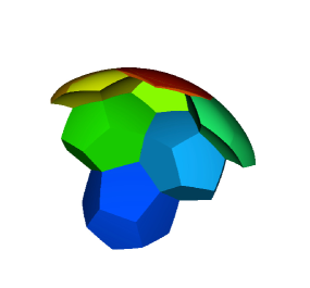
Figure 1. The Fundamental Domain (dark blue). We display $\mathcal{F}_{v}$ (in dark blue) and the projection $p$ in ${\mathbb{R}}^{3}$ of the images of $\mathcal{F}$ by six elements of $\mathcal{I}^{*}$. It is the representation of a part, included in ${\mathcal{B}}^{\prime}$, of the tiling of $\mathcal{S}^{3}$.

Obviously $\Psi$ is entirely determined on ${\mathbb{R}}_{t}\times\mathbf{K}$ by its restriction to ${\mathbb{R}}_{t}\times\mathcal{F}$, hence we are going to work on ${\mathbb{R}}_{t}\times\mathcal{F}_{v}$. We introduce the map $f:\;(x,y,z)\in\mathcal{F}_{v}\mapsto f(x,y,z)=\left(\sqrt{1-x^{2}-y^{2}-z^{2}},x,y,z\right)\in\mathcal{S}^{3}.$ $f$ is one-to-one from $\mathcal{F}_{v}\subset{\mathbb{R}}^{3}$ onto $\mathcal{F}\subset\mathcal{S}^{3}$ and we put

(II.13) $$u(t,x,y,z):=\Psi(t,f(x,y,z)).$$

It is clear that $\Phi\in H^{1}(\mathbf{K})$ iff $v:=\Phi\circ f$ belongs to the usual Sobolev space $H^{1}$ on $\mathcal{F}_{v}$ for the euclidean metric of ${\mathbb{R}}^{3}$, $H^{1}(\mathcal{F}_{v})=\{v\in L^{2}(\mathcal{F}_{v}),\;\;\nabla_{x,y,z}v\in L^{2}(\mathcal{F}_{v})\},$ and satisfies the boundary condition

$$\forall X,X^{\prime}\in\partial\mathcal{F}_{v},\;\;X\sim X^{\prime}\Rightarrow v(X)=v(X^{\prime}).$$

We deduce that $\Psi\in C^{0}\left({\mathbb{R}}_{t};H^{1}(\mathbf{K})\right)\cap C^{1}\left({\mathbb{R}}_{t};L^{2}(\mathbf{K})\right)$ is solution of (I.2) iff $u$ belongs to $C^{0}\left({\mathbb{R}}_{t};H^{1}(\mathcal{F}_{v})\right)\cap C^{1}\left({\mathbb{R}}_{t};L^{2}(\mathcal{F}_{v})\right)$ and satisfies the equation (I.8) where

(II.14) $$\Delta_{\mathcal{F}_{v}}=(1-x^{2})\,\partial_{11}^{2}+(1-y^{2})\,\partial_{22}^{2}+(1-z^{2})\,\partial_{33}^{2}-2xy\,\partial_{12}^{2}-2xz\,\partial_{13}^{2}-2yz\,\partial_{23}^{2}-3x\,\partial_{1}-3y\,\partial_{2}-3z\,\partial_{3},$$

and the boundary conditions

(II.15) $$\forall(t,X,X^{\prime})\in{\mathbb{R}}\times\partial\mathcal{F}_{v}\times\partial\mathcal{F}_{v},\;\;X\sim X^{\prime}\Rightarrow u(t,X)=u(t,X^{\prime}).$$

To handle the boundary when applying the finite element method, it is very convenient to take into account the boundary condition (II.15) by a suitable choice of the functional space. In the sequel we denote $X:=(x,y,z)$, $\mid X\mid^{2}:=x^{2}+y^{2}+z^{2}$ and $dX:=dx\,dy\,dz$. For $m=-1,0,1,$ we introduce the spaces $W^{m}(\mathcal{F}_{v})$ that are isometric to the spaces $H^{m}(\mathbf{K})$ :

(II.16) $$W^{m}(\mathcal{F}_{v}):=\left\{u=\Phi\circ f,\;\Phi\in H^{m}(\mathbf{K})\right\},\;\;\|u\|_{W^{m}}:=\|\Phi\|_{H^{m}}.$$

We have

(II.17) $$W^{0}(\mathcal{F}_{v}):=L^{2}(\mathcal{F}_{v},(1-\mid X\mid^{2})^{-\frac{1}{2}}dX),$$

(II.18) $$W^{1}(\mathcal{F}_{v}):=\left\{u\in H^{1}(\mathcal{F}_{v}),\;\;X\sim X^{\prime}\Rightarrow u(X)=u(X^{\prime})\right\},\;\|u\|_{W^{1}}^{2}=\sum_{\mid\alpha\mid\leq 1}\|\partial^{\alpha}u\|^{2}_{W^{0}(\mathcal{F}_{v})}.$$

Moreover $u\in C^{k}\left({\mathbb{R}}_{t},W^{m}(\mathcal{F}_{v})\right)$ iff $\Psi\in C^{k}\left({\mathbb{R}}_{t};H^{m}(\mathbf{K})\right)$ and Theorem II.1 can be expressed in terms of $u$ as the following

Theorem II.2.

Given $u_{0}\in W^{1}(\mathcal{F}_{v})$, $u_{1}\in W^{0}(\mathcal{F}_{v})$, $t^{*}\in{\mathbb{R}}$, there exists a unique $u$ solution of the equation (I.8) and satisfying

(II.19) $$u\in C^{0}\left({\mathbb{R}}_{t}^{+};W^{1}(\mathcal{F}_{v})\right)\cap C^{1}\left({\mathbb{R}}_{t}^{+};W^{0}(\mathcal{F}_{v})\right)\cap C^{2}\left({\mathbb{R}}_{t}^{+};W^{-1}(\mathcal{F}_{v})\right),$$

(II.20) $$u(t^{*},.)=u_{0}(.),\;\;\partial_{t}u(t^{*},.)=u_{1}(.).$$

$u$ is the unique function satisfying (II.19), (II.20) and such that for any $\phi\in W^{1}(\mathcal{F}_{v})$, we have:

$$0=\frac{d^{2}}{dt^{2}}\int_{\mathcal{F}_{v}} (1-\mid X\mid^{2})^{-\frac{1}{2}}u(t,X)\phi(X)\,dX+3\frac{a^{\prime}(t)}{a(t)}\frac{d}{dt}\int_{\mathcal{F}_{v}}(1-\mid X\mid^{2})^{-\frac{1}{2}}u(t,X)\phi(X)\,dX$$

(II.21) $$+\frac{1}{a^{2}(t)}\int_{{\mathcal{F}}_{v}} (1-\mid X\mid^{2})^{-\frac{1}{2}}$$

$$\left[\nabla_{X}u(t,X)\cdot\nabla_{X}\phi(X)-\left(X\cdot\nabla_{X}u(t,X)\right)\left(X\cdot\nabla_{X}\phi(X)\right)\right]dX$$

where $\nabla_{X}u=\left(\partial_{x}u,\partial_{y}u,\partial_{z}u\right)$, $dX=dxdydz$.

We end this part by discussing the possible horizons in the dynamical universe (I.1). We recall that the comoving spatial distance $d$ between any two points $x$ and $y$ on $\mathcal{S}^{3}$ is given by: $d(x,y)=\arccos[\delta_{ij}x^{i}y^{j}]$. $\mathcal{F}_{v}$ is endowed with the distance induced by $d$. Moreover the largest distance $d_{max}$ between the origin and the boundary of $\mathcal{F}_{v}$ is reached at any of its vertices. So we have $d_{max}=\arccos\left(\frac{\sigma^{2}}{2\sqrt{2}}\right)\simeq 0.388$. The metric on ${\mathbb{R}}_{t}\times\mathcal{F}_{v}$ can be expressed in spherical coordinates $\rho=\mid X\mid$, $\omega=\rho^{-1}X$, by $ds^{2}=dt^{2}-a^{2}(t)\left(\frac{1}{1-\rho^{2}}d\rho^{2}+\rho^{2}d\omega^{2}\right)$ where $\omega\in\mathcal{S}^{2}$, $0\leq\rho\leq\rho_{max}(\omega)$. We have

(II.22) $$R_{max}:=\sup_{\omega\in\mathcal{S}^{2}}\rho_{max}(\omega)=\sin(d_{max})=\sqrt{1-\frac{\sigma^{4}}{8}}\simeq 0.378.$$

Given $t^{*}\in{\mathbb{R}}$, $0\leq R<R_{max}$ we investigate the future causal domain $\mathcal{O}^{+}(t^{*},R)$ of $\{t^{*}\}\times(\mathcal{F}_{v}\cap([0\leq\rho\leq R]\times{\mathcal{S}}^{2}))$. Solving

(II.23) $$\frac{\rho^{\prime}(t)}{\sqrt{1-\rho^{2}(t)}}=\frac{1}{a(t)},$$

we get that

$$\mathcal{O}^{+}(t^{*},R)=\bigcup_{t\geq t^{*}}\{t\}\times(\mathcal{F}_{v}\cap([0\leq\rho\leq R(t)]\times{\mathcal{S}}^{2}))$$

where

(II.24) $$R(t)=\sin\left(\arcsin(R)+\int_{t^{*}}^{t}\frac{1}{a(s)}ds\right)$$

provided that $\arcsin(R)+\int_{t^{*}}^{t}\frac{1}{a(s)}ds\leq\pi/2$. Therefore an interesting phenomenon appears if

(II.25) $$\arcsin(R)+\int_{t^{*}}^{\infty}\frac{1}{a(s)}ds<\arcsin(R_{max})=d_{max}.$$

In this case, a future horizon exists:

(II.26) $$\mathcal{O}^{+}(t^{*},R)\subset[t^{*},\infty)\times[0,R_{h}]\times\mathcal{S}^{2},$$

where the radius of this future horizon is

(II.27) $$R_{h}:=\sin\left(\arcsin(R)+\int_{t^{*}}^{\infty}\frac{1}{a(s)}ds\right).$$

Returning to the scalar waves, we conclude that if $u_{0}$ and $u_{1}$ are supported in $\rho\leq R$, then for any $t\geq t^{*}$, $u(t)$ is supported in $\rho\leq R_{h}$.

Similarly, if $t_{ls}$ is the time of recombination, there exists a past horizon, called horizon sphere or last scattering surface, for an observer located at $t_{obs}>t_{ls}$. In the universal covering ${\mathcal{S}}^{3}$ of $\mathbf{K}$ described in spherical coodinates $(\xi,\theta,\varphi)$, it is the submanifold $\{\chi=\eta_{obs}-\eta_{ls}\}\times S^{2}_{\theta,\varphi}$ where $\eta$ is the conformal time,

(II.28) $$\eta_{obs}-\eta_{ls}=\int_{t_{ls}}^{t_{obs}}\frac{1}{a(s)}ds<d_{max}.$$

Then, the horizon sphere on which this observer can see the primordial plasma in the sky $S^{2}_{\theta,\varphi}$ has the radius

(II.29) $$R_{t_{ls},t_{obs}}:=\sin\left(\int_{t_{ls}}^{t_{obs}}\frac{1}{a(s)}ds\right).$$

If $\eta_{obs}-\eta_{ls}<d_{max}$ we have

(II.30) $$R_{t_{ls},t_{obs}}<R_{max}=\sqrt{1-\frac{\sigma^{4}}{8}}$$

hence the observable universe of radius $R_{t_{ls},t_{obs}}$ is strictly included in the whole universe ${\mathbf{K}}$. In this case, there is no multiple copies of images. In contrast, if

(II.31) $$R_{t_{ls},t_{obs}}>R_{max}=\sqrt{1-\frac{\sigma^{4}}{8}},$$

the horizon radius is larger that the injectivity radius. Then the horizon sphere wraps all the way around the universe and intersects itself. The case (II.31) has a great interest in cosmology: the observer could detect multiple images of radiating sources, some circles-in-the-sky appear, leading evidence of a non-trivial topology of the Universe [2], [27], [30], [36]. We present a numerical experiment of this situation in part 4.2.

Finally we give the expression of these quantities for the two accelerating universes that we consider, $d\mathcal{S}_{4}(\mathbf{K})$ and the inflationary spacetime. For $a(t)=H^{-1}\cosh(Ht)$, we have

$$R(t)=\sin\left(\arcsin R-2\arctan(e^{Ht^{\star}})+2\arctan(e^{Ht})\right),$$

(II.32) $$R_{t_{ls},t_{obs}}=\sin\left(2\arctan\left(e^{Ht_{obs}}\right)-2\arctan\left(e^{Ht^{\star}}\right)\right),$$

and if $a(t)=e^{t}$ we have

(II.33) $$R(t)=\sin\left(\arcsin R+e^{-t^{\star}}-e^{-t}\right),\;\;R_{t_{ls},t_{obs}}=\sin\left(e^{-t_{ls}}-e^{-t_{obs}}\right).$$

III. Asymptotic behaviours of smooth solutions

In this part, we investigate the asymptotic behaviour of the fields as $t\rightarrow+\infty$. We prove that the asymptotic profile $\Psi_{\infty}(.):=\lim_{t\rightarrow\infty}\Psi(t,.)$ exists if the scale factor is exponentially increasing. In the case of the de Sitter type universe $d\mathcal{S}_{4}(\mathbf{K})$, and in the case of the exponentially inflating model for which $a(t)=e^{t}$ we are able to compute its expression, and the first terms of the asymptotic expansion, in terms of the Cauchy data. Similar results have been obtained in [3] for the steady state universe $\left({\mathbb{R}}_{t}\times{\mathbb{R}}_{\mathrm{x}}^{3},\;ds^{2}=dt^{2}-e^{2t}d\mathrm{x}^{2}\right)$ (see also [33]).

III.1. Asymptotic profile.

We prove the existence of $\Psi_{\infty}$ if the scale factor is at least exponentially increasing, i.e. satisfies an assumption of the type:

(III.1) $$\exists\gamma>0,\;\;\exists t^{*}\in{\mathbb{R}},\;\;\forall t\geq t^{*}\;\;\gamma\leq\frac{a^{\prime}(t)}{a(t)}.$$

Theorem III.1.

We assume (III.1) is satisfied. Then for any finite energy solution $\Psi$ of (I.2), the energy (I.7) is exponentially decreasing

(III.2) $$\forall t\geq t^{*},\;\;E(\Psi,t)\leq e^{-2\gamma(t-t^{*})}E(\Psi,t^{*}),$$

and there exists $\Psi_{\infty}\in L^{2}(\mathbf{K})$ such that

(III.3) $$\forall t\geq t^{*},\;\;\|\Psi(t)-\Psi_{\infty}\|_{L^{2}(\mathbf{K})}\lesssim e^{-\gamma t}E^{\frac{1}{2}}(\Psi,t^{*}).$$

Proof. (II.4) and (III.1) imply that $dE(\Psi,t)/dt\leq-2\gamma E(\Psi,t)$, hence (III.2) is proved. To establish the existence of the profile $\Psi_{\infty}$, our method relies on the spectral expansion of $\Psi(t,.)$ and the energy estimate (or an explicit resolution) for the ODE. More precisely, since the Laplace-Beltrami operator $\Delta_{\mathbf{K}}$ on $\mathbf{K}$ is a non positive, self-adjoint elliptic operator on a compact manifold, its spectrum is a discrete set of eigenvalues $-q^{2}\leq 0$. Moreover, by the Hilbert-Schmidt theorem there exists an orthonormal basis in $L^{2}(\mathbf{K})$, formed of eigenfunctions $\left(\Psi_{q}\right)_{q}\subset H^{1}(\mathbf{K})$ associated to $q^{2}$, i.e.

(III.4) $$-\Delta_{\mathbf{K}}\Psi_{q}=q^{2}\Psi_{q}.$$

Moreover the eigenvalues are explicitly known (see [1, 17, 20, 21]). One has:

(III.5) $$0\leq q,\;\;q^{2}=\beta^{2}-1,$$

(III.6) $$\mbox{with }\beta\in\{1,13,21,25,31,33,37,41,43,45,49,51,53,55,57\}\cup\{2n+1,\,n\geq 30\}.$$

In particular, since the volume of $\mathbf{K}$ is $\pi^{2}/60$ (see e.g. [14] p. 5160), we have:

(III.7) $$\Psi_{0}(X)=\frac{2\sqrt{15}}{\pi}.$$

Any finite energy solution $\Psi(t,X)$ of equation (I.2) has an expansion of the form

(III.8) $$\Psi(t,X)=\sum_{q}u_{q}(t)\Psi_{q}(X),\;\;t\in{\mathbb{R}},\;\;X\in\mathbf{K},$$

where $u_{q}$ is solution of the ordinary differential equation

(III.9) $$u_{q}^{\prime\prime}+3\frac{a^{\prime}(t)}{a(t)}u^{\prime}+\frac{q^{2}}{a^{2}(t)}u_{q}=0.$$

For the finite energy solution we have

(III.10) $$E(\Psi,t)=\sum_{q}\left|u^{\prime}_{q}(t)\right|^{2}+\frac{q^{2}}{a^{2}(t)}\left|u_{q}(t)\right|^{2},\;\;\sum_{q}\left|u^{\prime}_{q}(t)\right|^{2}+q^{2}\left|u_{q}(t)\right|^{2}<\infty,$$

and if $\Psi$ is a smooth solution we have

$$\forall k,p\in{\mathbb{N}},\;\;\sum_{q}q^{p}\left|\frac{d^{k}}{dt^{k}}u_{q}(t)\right|<\infty.$$

These series converge locally uniformly with respect to $t$. Now, multiplying (III.9) by $u^{\prime}_{q}$, we get an energy type equality:

$$\mid u^{\prime}_{q}(t)\mid^{2}+\frac{q^{2}}{a^{2}(t)}\mid u_{q}(t)\mid^{2}=-2\frac{a^{\prime}(t)}{a(t)}\left(3\mid u^{\prime}_{q}(t)\mid^{2}+\frac{q^{2}}{a^{2}(t)}\mid u_{q}(t)\mid^{2}\right).$$

We get from hypothese (III.1) that

$$\frac{d}{dt}\left(\mid u^{\prime}_{q}(t)\mid^{2}+\frac{q^{2}}{a^{2}(t)}\mid u_{q}(t)\mid^{2}\right)\leq-2\gamma\left(\mid u^{\prime}_{q}(t)\mid^{2}+\frac{q^{2}}{a^{2}(t)}\mid u_{q}(t)\mid^{2}\right),$$

hence

$$\mid u^{\prime}_{q}(t)\mid^{2}+\frac{q^{2}}{a^{2}(t)}\mid u_{q}(t)\mid^{2}\leq e^{-2\gamma(t-t^{*})}\left(\mid u^{\prime}_{q}(t^{*})\mid^{2}+\frac{q^{2}}{a^{2}(t^{*})}\mid u_{q}(t^{*})\mid^{2}\right),$$

and we deduce that for any $t\geq t^{*}$ we have:

(III.11) $$\mid u^{\prime}_{q}(t)\mid\leq e^{-\gamma t}\left(\mid u^{\prime}_{q}(t^{*})\mid^{2}+\frac{q^{2}}{a^{2}(t^{*})}\mid u_{q}(t^{*})\mid^{2}\right)^{\frac{1}{2}}.$$

Therefore we can introduce

$$u_{q}(\infty):=u_{q}(t^{*})+\int_{t^{*}}^{\infty}u^{\prime}_{q}(t)dt,\;\;\Psi_{\infty}:=\sum_{q}u_{q}(\infty)\Psi_{q}.$$

Now (III.3) follows from (III.10) and (III.11).

$\square$

We compute $\Psi_{\infty}$ in the next sections. We remark that the profile $\Psi_{\infty}(.)$ is more regular than the field $\Psi(t,.)$. In short, the Theorems III.39 and III.58 show that $\Psi_{\infty}\in H^{m+1}$ if $\Psi(0,.)\in H^{m}$, $\partial_{t}\Psi(0,.)\in H^{m-1}$. This phenomenon has been noticed in the case of the steady-state universe [3].

III.2. $d\mathcal{S}_{4}(\mathbf{K})$ universe.

We consider the $d\mathcal{S}_{4}(\mathbf{K})$ universe for which $a(t)=H^{-1}\cosh(Ht)$. We calculate an explicit expression of the asymptotic profile and we prove that $\Delta_{\mathbf{K}}\Psi(t)-\frac{1}{2H}\left(1-\tanh Ht\right)^{-1}\partial_{t}\Psi(t)$ tends to zero.

Theorem III.2.

Given a smooth solution $\Psi$ of (I.2), there exist constants $A^{+}_{q}$ and $A^{-}_{q}$ depending only on the initial data such that

(III.12) $$\begin{split}\Psi(t,X)=&\left[-\sqrt{\frac{2}{\pi}}A^{+}_{0}+\left(\cosh Ht\right)^{-\frac{3}{2}}A^{-}_{0}\mathrm{P}^{-\frac{3}{2}}_{\frac{1}{2}}(\tanh Ht)\right]\Psi_{0}(X)\\ &+\left(\cosh Ht\right)^{-\frac{3}{2}}\sum_{q\neq 0}\left[A^{+}_{q}\mathrm{P}^{\frac{3}{2}}_{\beta-\frac{1}{2}}(\tanh Ht)+A^{-}_{q}\mathrm{Q}^{\frac{3}{2}}_{\beta-\frac{1}{2}}(\tanh Ht)\right]\Psi_{q}(X),\end{split}$$

(III.13) $$\Psi_{\infty}(X)=-\sqrt{\frac{2}{\pi}}\sum_{q}A^{+}_{q}\Psi_{q}(X),$$

(III.14) $$\Psi(t,X)-\Psi_{\infty}(X)=-\sqrt{\frac{2}{\pi}}\sum_{q\neq 0}q^{2}A^{+}_{q}\Psi_{q}(X)\left(1-\tanh Ht\right)+0\left(\left(1-\tanh Ht\right)^{\frac{3}{2}}\right),$$

(III.15) $$\begin{split}\Delta_{\mathbf{K}}\Psi(t,X)-&\frac{1}{2H}\left(1-\tanh Ht\right)^{-1}\partial_{t}\Psi(t,X)=\frac{2}{\sqrt{\pi}}A^{-}_{0}\left(1-\tanh Ht\right)^{\frac{1}{2}}\\ &\qquad+\sqrt{\frac{2}{\pi}}\left[\sum_{q\neq 0}q^{2}(q^{2}+\frac{3}{4})A^{+}_{q}\Psi_{q}(X)\right]\left(1-\tanh Ht\right)+0\left(1-\tanh Ht\right)^{\frac{3}{2}}\end{split}$$

where $q$ and $\beta$ are given by equation (III.5), equation (III.6). The coefficients $A_{q}^{\pm}$ are given by

(III.16) $$A^{+}_{0}=-\sqrt{\frac{\pi}{2}}\left(u_{0}(0)+\frac{\pi}{4}u^{\prime}(0)\right),\;\;A^{+}_{q}=-\sqrt{\frac{\pi}{2}}\,\frac{\sin\left(\frac{\pi}{2}\sqrt{q^{2}+1}\right)}{\sqrt{q^{2}+1}}u_{q}(0),\;q\neq 0,$$

(III.17) $$A_{0}^{-}=-\sqrt{\frac{\pi}{2}}u_{0}^{\prime}(0),\;\;A^{-}_{q}=-\sqrt{\frac{2}{\pi}}\,\frac{\sin\left(\frac{\pi}{2}\sqrt{q^{2}+1}\right)}{q^{2}}u^{\prime}_{q}(0),\;q\neq 0,$$

where $u_{q}(t):=<\Psi(t,.),\Psi_{q}>_{L^{2}(\mathbf{K})}$.

Proof. The differential equation (III.9) has the form:

(III.18) $$u^{\prime\prime}_{q}(t)+3H\tanh(Ht)\,u^{\prime}_{q}(t)+\frac{q^{2}H^{2}}{\cosh^{2}(Ht)}u_{q}(t)=0.$$

For each $q$ we introduce a new function $w_{q}$ defined by

$$u_{q}(t):=(\cosh Ht)^{-\frac{3}{2}}\,w_{q}(t).$$

Then $u_{q}$ satisfies equation (III.18) iff $w_{q}$ is solution of

(III.19) $$H^{-2}w_{q}^{\prime\prime}(t)+\left((q^{2}+\frac{3}{4})\cosh^{-2}(Ht)-\frac{9}{4}\right)w_{q}(t)=0.\;$$

Now we put $w_{q}(t)=\tilde{w}_{q}(\tanh Ht)$. Thanks to the relation $q^{2}+\frac{3}{4}=(\beta-\frac{1}{2})(\beta+\frac{1}{2})$ we deduce that $w_{q}$ satisfies equation (III.19) iff $\tilde{w}_{q}$ is solution of the associated Legendre equation

(III.20) $$(1-x^{2})\tilde{w}^{\prime\prime}_{q}(x)-2x\tilde{w}^{\prime}_{q}(x)+\left(\nu(\nu+1)-\frac{\mu^{2}}{1-x^{2}}\right)\tilde{w}_{q}(x)=0,$$

where $\nu=\beta-\frac{1}{2}$, $\mu=\pm\frac{3}{2}$ and $x\in]-1,+1[$. In the sequel, we use several formulae, all from [29]. The first eigenvalue $q=0$ is a particular case where $\nu=\frac{1}{2}$. Thanks to formula 14.2.7 the Wronskian of $\mathrm{P}^{-\frac{3}{2}}_{\frac{1}{2}}(x)$ and $\mathrm{P}^{\frac{3}{2}}_{\frac{1}{2}}(x)$ is not zero. For the other eigenvalues, $\beta$ is greater than $13$ and is an odd integer. So $\mathrm{Q}^{\frac{3}{2}}_{\beta-\frac{1}{2}}$ is defined and, thanks to formula 14.2.4, the Wronskian of $\mathrm{P}^{\frac{3}{2}}_{\beta-\frac{1}{2}}(x)$ and $\mathrm{Q}^{\frac{3}{2}}_{\beta-\frac{1}{2}}(x)$ is not zero. So there exist constants $A^{+}_{q}$ and $A^{-}_{q}$ depending on initial data such that

$$\tilde{w}_{0}(x)=A^{+}_{0}\mathrm{P}^{\frac{3}{2}}_{\frac{1}{2}}(x)+A^{-}_{0}\mathrm{P}^{-\frac{3}{2}}_{\frac{1}{2}}(x),\;\mbox{and }\;\tilde{w}_{q}(x)=A^{+}_{q}\mathrm{P}^{\frac{3}{2}}_{\beta-\frac{1}{2}}(x)+A^{-}_{q}\mathrm{Q}^{\frac{3}{2}}_{\beta-\frac{1}{2}}(x)\;\mbox{for }q\neq 0.$$

Then

(III.21) $$u_{0}(t)=\left(\cosh Ht\right)^{-\frac{3}{2}}\left[A^{+}_{0}\mathrm{P}^{\frac{3}{2}}_{\frac{1}{2}}(\tanh Ht)+A^{-}_{0}\mathrm{P}^{-\frac{3}{2}}_{\frac{1}{2}}(\tanh Ht)\right],$$

(III.22) $$u_{q}(t)=\left(\cosh Ht\right)^{-\frac{3}{2}}\left[A^{+}_{q}\mathrm{P}^{\frac{3}{2}}_{\beta-\frac{1}{2}}(\tanh Ht)+A^{-}_{q}\mathrm{Q}^{\frac{3}{2}}_{\beta-\frac{1}{2}}(\tanh Ht)\right]\;\mbox{for }q\neq 0.$$

To obtain asymptotic profiles we use hypergeometric representation of the Ferrers functions (see formulae 14.3.i). We recall that for $x\in]-1,+1[$

$$\mathrm{P}^{\mu}_{\nu}(x) =\left(\frac{1+x}{1-x}\right)^{\frac{\mu}{2}}\mathbf{F}(\nu+1,-\nu;1-\mu;\frac{1}{2}-\frac{1}{2}x)$$

$$=\left(\frac{1+x}{1-x}\right)^{\frac{\mu}{2}}\sum_{s=0}^{+\infty}\frac{(\nu+1)_{s}(-\nu)_{s}}{\Gamma(1-\mu+s)}\frac{1}{s!}\left(\frac{1}{2}\right)^{s}(1-x)^{s},$$

where $(\alpha)_{n}$ is the Pochhammer’s symbol: $\alpha(\alpha+1)(\alpha+2)\textperiodcentered\textperiodcentered\textperiodcentered(\alpha+n-1)$ if $n=1,2,3,...$, and $1$ if $n=0$. First we consider the case $q\neq 0$, that is $\nu=\beta-\frac{1}{2}\neq\frac{1}{2}$. For $t$ in the neighbourhood of $+\infty$, the regularity of the previous series at $0$ leads to

$$\mathrm{P}^{\frac{3}{2}}_{\nu}(\tanh Ht)= \left(\frac{1+\tanh Ht}{1-\tanh Ht}\right)^{\frac{3}{4}}\,\left[\frac{1}{\Gamma(-\frac{1}{2})}+\frac{(\nu+1)(-\nu)}{2\Gamma(\frac{1}{2})}\left(1-\tanh Ht\right)\right.$$

$$\left.+\frac{(\nu+1)(\nu+2)(-\nu)(-\nu+1)}{8\Gamma(\frac{3}{2})}\left(1-\tanh Ht\right)^{2}+0\left(\left(1-\tanh Ht\right)^{3}\right)\right].$$

So

(III.23) $$\left(\cosh Ht\right)^{-\frac{3}{2}}\mathrm{P}^{\frac{3}{2}}_{\beta-\frac{1}{2}}(\tanh Ht) =\left(1+\tanh Ht\right)^{\frac{3}{2}}\,\left[\frac{1}{\Gamma(-\frac{1}{2})}-(\beta^{2}-\frac{1}{4})\frac{1}{2\Gamma(\frac{1}{2})}\left(1-\tanh Ht\right)\right.$$

$$\left.+\frac{(\beta^{2}-\frac{1}{4})(\beta^{2}-\frac{9}{4})}{8\Gamma(\frac{3}{2})}\left(1-\tanh Ht\right)^{2}+0\left(\left(1-\tanh Ht\right)^{3}\right)\right].$$

Likewise for $x\in]-1,+1[$

$$\mathrm{Q}^{\frac{3}{2}}_{\beta-\frac{1}{2}}(x) =\frac{\pi}{2\sin(\frac{3}{2}\pi)}\left(\cos(\frac{3}{2}\pi)\left(\frac{1+x}{1-x}\right)^{\frac{3}{4}}\mathbf{F}(\nu+1,-\nu;-\frac{1}{2};\frac{1}{2}-\frac{1}{2}x)\right.$$

$$\qquad\qquad\qquad\left.-\frac{\Gamma(\nu+\frac{5}{2})}{\Gamma(\nu-\frac{1}{2})}\left(\frac{1-x}{1+x}\right)^{\frac{3}{4}}\mathbf{F}(\nu+1,-\nu;\frac{5}{2};\frac{1}{2}-\frac{1}{2}x)\right)$$

$$=\frac{\pi}{2}\frac{\Gamma(\nu+\frac{5}{2})}{\Gamma(\nu-\frac{1}{2})}\left(\frac{1-x}{1+x}\right)^{\frac{3}{4}}\sum_{s=0}^{+\infty}\frac{(\nu+1)_{s}(-\nu)_{s}}{\Gamma(\frac{5}{2}+s)}\frac{1}{s!}\left(\frac{1}{2}\right)^{s}(1-x)^{s}.$$

Then, for $t$ in the neighbourhood of $+\infty$ we have

$$\begin{split}\mathrm{Q}^{\frac{3}{2}}_{\beta-\frac{1}{2}}(\tanh Ht)&=\frac{\pi}{2}\frac{\Gamma(\beta+2)}{\Gamma(\beta-1)}\\ &\left(\frac{1-\tanh Ht}{1+\tanh Ht}\right)^{\frac{3}{4}}\left[\frac{1}{\Gamma(\frac{5}{2})}-(\beta^{2}-\frac{1}{4})\frac{1}{2\Gamma(\frac{7}{2})}\left(1-\tanh Ht\right)+0\left(\left(1-\tanh Ht\right)^{2}\right)\right],\end{split}$$

and so

(III.24) $$\left(\cosh Ht\right)^{-\frac{3}{2}}\mathrm{Q}^{\frac{3}{2}}_{\beta-\frac{1}{2}}(\tanh Ht)=\frac{\pi}{2}\frac{1}{\Gamma(\frac{5}{2})}\frac{\Gamma(\beta+2)}{\Gamma(\beta-1)}\left(1-\tanh Ht\right)^{\frac{3}{2}}+0\left(\left(1-\tanh Ht\right)^{\frac{5}{2}}\right).$$

From equation (III.22), equation (III.23) and equation (III.24) we deduce for $t\rightarrow+\infty$ and $q\neq 0$

$$u_{q}(t)=-A^{+}_{q}\frac{1}{2\sqrt{\pi}}\left(1+\tanh Ht\right)^{\frac{3}{2}}-A^{+}_{q}\frac{\sqrt{\pi}}{2}(\beta^{2}-\frac{1}{4})\left(1+\tanh Ht\right)^{\frac{3}{2}}\left(1-\tanh Ht\right)$$

$$\;+0\left(\left(1-\tanh Ht\right)^{\frac{5}{2}}\right).$$

Hence we have got for $q\neq 0$

(III.25) $$u_{q}(t)\sim-A^{+}_{q}\sqrt{\frac{2}{\pi}},{\mbox{ and }}\;u_{q}(t)+A^{+}_{q}\sqrt{\frac{2}{\pi}}=-q^{2}A^{+}_{q}\sqrt{\frac{2}{\pi}}\left(1-\tanh Ht\right)+0\left(\left(1-\tanh Ht\right)^{\frac{3}{2}}\right).$$

Using formula 14.10.4 we deduce derivatives of $u_{q}$ from equation (III.22). For $q\neq 0$ we have

(III.26) $$u^{\prime}_{q}(t) =H\left(\cosh Ht\right)^{-\frac{3}{2}}\left(\tanh Ht\right)(\beta-1)\left[A^{+}_{q}\mathrm{P}^{\frac{3}{2}}_{\beta-\frac{1}{2}}(\tanh Ht)+A^{-}_{q}\mathrm{Q}^{\frac{3}{2}}_{\beta-\frac{1}{2}}(\tanh Ht)\right]$$

$$\qquad-H\left(\cosh Ht\right)^{-\frac{3}{2}}(\beta-1)\left[A^{+}_{q}\mathrm{P}^{\frac{3}{2}}_{\beta+\frac{1}{2}}(\tanh Ht)+A^{-}_{q}\mathrm{Q}^{\frac{3}{2}}_{\beta+\frac{1}{2}}(\tanh Ht)\right]$$

$$=H\left(\cosh Ht\right)^{-\frac{3}{2}}(\beta-1)A^{+}_{q}\left[\left(\tanh Ht\right)\mathrm{P}^{\frac{3}{2}}_{\beta-\frac{1}{2}}(\tanh Ht)-\mathrm{P}^{\frac{3}{2}}_{\beta+\frac{1}{2}}(\tanh Ht)\right]$$

$$\qquad+H\left(\cosh Ht\right)^{-\frac{3}{2}}(\beta-1)A^{-}_{q}\left[\left(\tanh Ht\right)\mathrm{Q}^{\frac{3}{2}}_{\beta-\frac{1}{2}}(\tanh Ht)-\mathrm{Q}^{\frac{3}{2}}_{\beta+\frac{1}{2}}(\tanh Ht)\right].$$

And from equation (III.26), equation (III.23) and equation (III.24) we deduce for $\nu=\beta-\frac{1}{2}\neq\frac{1}{2}$ and $t\rightarrow+\infty$

$$\begin{split}&u^{\prime}_{q}(t)=H(\beta-1)A^{+}_{q}\left(1+\tanh Ht\right)^{\frac{3}{2}}\\ &\quad\left[\frac{1}{\Gamma(-\frac{1}{2})}\left(-1+\tanh Ht\right)+\left(-(\beta^{2}-\frac{1}{4})\tanh Ht+(\beta+\frac{3}{2})(\beta+\frac{1}{2})\right)\frac{1}{2\Gamma(\frac{1}{2})}\left(1-\tanh Ht\right)\right.\\ &\qquad\qquad\left.+\left((\beta^{2}-\frac{1}{4})(\beta^{2}-\frac{9}{4})\tanh Ht-(\beta+\frac{3}{2})(\beta+\frac{5}{2})(\beta^{2}-\frac{1}{4})\right)\frac{1}{8\Gamma(\frac{3}{2})}\left(1-\tanh Ht\right)^{2}\right]\\ &\qquad\qquad+0\left(\left(1-\tanh Ht\right)^{\frac{5}{2}}\right).\end{split}$$

That is for $q\neq 0$

$$\begin{split}u^{\prime}_{q}(t)&=A^{+}_{q}\frac{H}{\sqrt{\pi}}(\beta^{2}-1)\left(1+\tanh Ht\right)^{\frac{3}{2}}\\ &\qquad\left[\left(1-\tanh Ht\right)-(\beta^{2}-\frac{1}{4})\left(1-\tanh Ht\right)^{2}+0\left(1-\tanh Ht\right)^{\frac{5}{2}}\right],\end{split}$$

and then

$$\begin{split}-2Hq^{2}u_{q}(t)-&\left(1-\tanh Ht\right)^{-1}u^{\prime}_{q}(t)=\\ &q^{2}(q^{2}+\frac{3}{4})A^{+}_{q}\frac{H}{\sqrt{\pi}}\left(1+\tanh Ht\right)^{\frac{3}{2}}\left(1-\tanh Ht\right)+0\left(1-\tanh Ht\right)^{\frac{3}{2}}.\end{split}$$

It only remains to consider the case $q=0$. Actually $u_{0}$ can be written more simply by explaining $\mathrm{P}^{\frac{3}{2}}_{\frac{1}{2}}$. We use formula 14.10.4 : $(1-x^{2})\left(\mathrm{P}^{\frac{3}{2}}_{\frac{1}{2}}\right)^{\prime}(x)=(\frac{3}{2}-\frac{1}{2}-1)\mathrm{P}^{\frac{3}{2}}_{\frac{3}{2}}(x)+\frac{3}{2}x\mathrm{P}^{\frac{3}{2}}_{\frac{1}{2}}(x)=\frac{3}{2}x\mathrm{P}^{\frac{3}{2}}_{\frac{1}{2}}(x)$. So $\mathrm{P}^{\frac{3}{2}}_{\frac{1}{2}}$ has the form $C\left(1-x^{2}\right)^{-\frac{3}{4}}$ where $C$ is a constant. Since $\mathrm{P}^{\frac{3}{2}}_{\frac{1}{2}}(0)=\mathbf{F}(\frac{3}{2},-\frac{1}{2};-\frac{1}{2};\frac{1}{2})=-\sqrt{\frac{2}{\pi}}$ we can write $\mathrm{P}^{\frac{3}{2}}_{\frac{1}{2}}(x)=-\sqrt{\frac{2}{\pi}}\left(1-x^{2}\right)^{-\frac{3}{4}}$. So with equation (III.22) we obtain a new expression of $u_{0}$:

$$u_{0}(t)=-\sqrt{\frac{2}{\pi}}A^{+}_{0}+\left(\cosh Ht\right)^{-\frac{3}{2}}A^{-}_{0}\mathrm{P}^{-\frac{3}{2}}_{\frac{1}{2}}(\tanh Ht).$$

Moreover the hypergeometric representation of $\mathrm{P}^{-\frac{3}{2}}_{\frac{1}{2}}$ gives us for $t$ at $+\infty$

$$\begin{split}\left(\cosh Ht\right.&\left.\right)^{-\frac{3}{2}}\mathrm{P}^{-\frac{3}{2}}_{\frac{1}{2}}(\tanh Ht)=\\ \left(1-\tanh Ht\right)^{\frac{3}{2}}\left[\frac{1}{\Gamma(\frac{5}{2})}-\frac{3}{8}\frac{1}{\Gamma(\frac{7}{2})}\left(1-\tanh Ht\right)-\frac{15}{128}\frac{1}{\Gamma(\frac{9}{2})}\left(1-\tanh Ht\right)^{2}+0\left(\left(1-\tanh Ht\right)^{3}\right)\right],\end{split}$$

so

(III.27) $$u_{0}(t)=-\sqrt{\frac{2}{\pi}}A^{+}_{0}+A^{-}_{0}\frac{1}{\Gamma(\frac{5}{2})}\left(1-\tanh Ht\right)^{\frac{3}{2}}+0\left(\left(1-\tanh Ht\right)^{\frac{5}{2}}\right).$$

Then equation (III.25) and equation (III.27) prove equation (III.14). On the other hand we can simplify $u^{\prime}_{0}$ since $\mathrm{P}^{-\frac{3}{2}}_{\frac{3}{2}}$ has a simple writting (see formula 14.5.18 with $\theta\in]0,\pi[$ such that $\cos\theta=\tanh Ht$). We have:

$$\begin{split}u^{\prime}_{0}(t)&=-3H\left(\cosh Ht\right)^{-\frac{3}{2}}A^{-}_{0}\mathrm{P}^{-\frac{3}{2}}_{\frac{3}{2}}(\tanh Ht)\\ &=-3H\left(\cosh Ht\right)^{-\frac{3}{2}}\frac{1}{2^{\frac{3}{2}}}\frac{1}{\Gamma(\frac{3}{2}+1)}A^{-}_{0}\left(\sin\theta\right)^{\frac{3}{2}}=H\sqrt{\frac{2}{\pi}}\left(\cosh Ht\right)^{-3}A^{-}_{0}\\ &=-H\sqrt{\frac{2}{\pi}}A^{-}_{0}\left(1+\tanh Ht\right)^{\frac{3}{2}}\left(1-\tanh Ht\right)^{\frac{3}{2}},\end{split}$$

so

$$-\frac{1}{2H}\left(1-\tanh Ht\right)^{-1}u^{\prime}_{0}(t)=\frac{1}{\sqrt{2\pi}}A^{-}_{0}\left(1+\tanh Ht\right)^{\frac{3}{2}}\left(1-\tanh Ht\right)^{\frac{1}{2}}.$$

Finally to compute $A_{q}^{\pm}$ we remark that since $\beta=\sqrt{q^{2}+1}$ is an odd integer number, we have

(III.28) $$\mathrm{P}^{-\frac{3}{2}}_{\frac{1}{2}}(0)=\frac{1}{2}\sqrt{\frac{\pi}{2}},\;\left(\mathrm{P}^{-\frac{3}{2}}_{\frac{1}{2}}\right)^{\prime}(0)=-\sqrt{\frac{2}{\pi}},$$

(III.29) $$\mathrm{P}^{\frac{3}{2}}_{\beta-\frac{1}{2}}(0)=-\sqrt{\frac{2}{\pi}}\beta\sin\left(\beta\frac{\pi}{2}\right),\;\left(\mathrm{P}^{\frac{3}{2}}_{\beta-\frac{1}{2}}\right)^{\prime}(0)=0,$$

(III.30) $$\mathrm{Q}^{\frac{3}{2}}_{\beta-\frac{1}{2}}(0)=0,\;\left(\mathrm{Q}^{\frac{3}{2}}_{\beta-\frac{1}{2}}\right)^{\prime}(0)=-\sqrt{\frac{\pi}{2}}q^{2}\sin\left(\beta\frac{\pi}{2}\right).$$

The expressions of the coefficients follows from (III.12) by elementary computations. The proof is complete.

$\square$

We deduce from this theorem that any smooth solution $\Psi$ can be expressed as

$$\Psi(t,X)=\Psi^{+}(t,X)+\Psi^{-}(t,X),$$

where $\Psi^{+}$ and $\Psi^{-}$ are smooth solutions satisfying

(III.31) $$\Psi^{+}(t,X)=\Psi_{\infty}(X)+O\left(e^{-Ht}\right),$$

(III.32) $$\Psi^{-}(t,X)=O\left(e^{-\frac{3}{2}Ht}\right).$$

It is sufficient to define

(III.33) $$\Psi^{+}(t,X):=-\sqrt{\frac{2}{\pi}}A^{+}_{0}\Psi_{0}(X)+\left(\cosh Ht\right)^{-\frac{3}{2}}\sum_{q\neq 0}A^{+}_{q}\mathrm{P}^{\frac{3}{2}}_{\beta-\frac{1}{2}}(\tanh Ht)\Psi_{q}(X),$$

(III.34) $$\Psi^{-}(t,X):=\left(\cosh Ht\right)^{-\frac{3}{2}}\left[A^{-}_{0}\mathrm{P}^{-\frac{3}{2}}_{\frac{1}{2}}(\tanh Ht)\Psi_{0}(X)+\sum_{q\neq 0}A^{-}_{q}\mathrm{Q}^{\frac{3}{2}}_{\beta-\frac{1}{2}}(\tanh Ht)\Psi_{q}(X)\right].$$

We express the initial data for $\Psi^{\pm}$ in terms of those of $\Psi$, and we estimate the norms of $\Psi_{\infty}$.

Theorem III.3.

The smooth solutions $\Psi$, $\Psi^{\pm}$ and the asymptotic profile $\Psi_{\infty}$ satisfy :

(III.35) $$\Psi^{+}(0,X)=\Psi(0,X)+\frac{\pi}{4}<\partial_{t}\Psi(0,.),\Psi_{0}>_{L^{2}(\mathbf{K})}\Psi_{0}(X),\;\partial_{t}\Psi^{+}(0,X)=0,$$

(III.36) $$\Psi^{-}(0,X)=-\frac{\pi}{4}<\partial_{t}\Psi(0,.),\Psi_{0}>_{L^{2}(\mathbf{K})}\Psi_{0}(X),\;\;\partial_{t}\Psi^{-}(0,X)=\partial_{t}\Psi(0,X),$$

(III.37) $$\Psi_{\infty}=\left(-\Delta_{\mathbf{K}}+1\right)^{-\frac{1}{2}}\sin\left(\frac{\pi}{2}\sqrt{-\Delta_{\mathbf{K}}+1}\right)\Psi^{+}(0,.),$$

(III.38) $$\|\Psi_{\infty}\|_{L^{2}(\mathbf{K})}=\|\Psi^{+}(0,.)\|_{H^{-1}(\mathbf{K})},$$

(III.39) $$\|\nabla_{\mathbf{K}}\Psi_{\infty}\|_{H^{m}(\mathbf{K})}=\|\nabla_{\mathbf{K}}\Psi^{+}(0,.)\|_{H^{m-1}(\mathbf{K})}=\|\nabla_{\mathbf{K}}\Psi(0,.)\|_{H^{m-1}(\mathbf{K})},\;m=0,1.$$

In (III.37), the pseudodifferential operator $f\left(\Delta_{\mathbf{K}}\right)$ is defined by the usual functional calculus of the spectral theory: $f\left(\Delta_{\mathbf{K}}\right)\Phi$ is defined by $<f\left(\Delta_{\mathbf{K}}\right)\Phi,\Psi_{q}>_{L^{2}(\mathbf{K})}=f(-q^{2})<\Phi,\Psi_{q}>_{L^{2}(\mathbf{K})}$. We note that (III.5) assures that $\sin\left(\frac{\pi}{2}\sqrt{q^{2}+1}\right)\in\{+1,\,-1\}$.

Proof. We obtain (III.35) and (III.36) from (III.28), (III.29) and (III.30). We get (III.37) by (III.35) and the equalities

$$\Psi^{+}(0,X)=-\sqrt{\frac{2}{\pi}}\sum_{q}\beta\sin\left(\beta\frac{\pi}{2}\right)A^{+}_{q}\Psi_{q}=\sqrt{-\Delta_{\mathbf{K}}+1}\sin\left(\frac{\pi}{2}\sqrt{-\Delta_{\mathbf{K}}+1}\right)\Psi_{\infty}.$$

Finally since $\sin\left(\beta\frac{\pi}{2}\right)=\pm 1$, (III.38) and (III.39) follow from (III.35) and (III.37).

$\square$

We remark that $\Psi^{-}=0$ iff $\partial_{t}\Psi(0,.)=0$, and the asymptotic profile $\Psi_{\infty}$ depends only on $\Psi^{+}(0,.)$, therefore it is determined by $\Psi(0,.)$ and $\int_{\mathbf{K}}\partial_{t}\Psi(0,.)$. Moreover the map

$$S:\;\Psi^{+}(0,.)\longmapsto\Psi_{\infty}$$

is an isomorphism from $H^{-1}(\mathbf{K})$ onto $L^{2}(\mathbf{K})$ and from $L^{2}(\mathbf{K})$ onto $H^{1}(\mathbf{K})$. Since $S$ is a pseudodifferential operator given by $\left(-\Delta_{\mathbf{K}}+1\right)^{-\frac{1}{2}}\sin\left(\frac{\pi}{2}\sqrt{-\Delta_{\mathbf{K}}+1}\right)$, the computation of the asymptotic profile using this formula is a very hard task. In contrast, the numerical method for the computation of the time dependent field $\Psi(t,.)$ presented in the next part, allows to find $\Psi_{\infty}(X)=\lim_{t\rightarrow+\infty}\Psi(t,X)$ with a good accuracy.

III.3. Inflating universe.

We consider the toy model of an exponentially inflating universe with $a(t)=e^{t}$. We calculate the asymptotic profile of a wave $\Psi$ and we show that $\Delta_{\mathbf{K}}\Psi(t)-e^{2t}\partial_{t}\Psi(t)$ tends to zero.

Theorem III.4.

Given a smooth solution $\Psi$ of equation (I.2), there exist constants $A^{+}_{q}$ and $A^{-}_{q}$ depending only on initial data such that

(III.40) $$\Psi(t,X)=\left[A^{-}_{0}e^{-3t}+A^{+}_{0}\right]\Psi_{0}(X)+e^{-\frac{3}{2}t}\sum_{q\neq 0}\left[A^{-}_{q}J_{\frac{3}{2}}(qe^{-t})+A^{+}_{q}Y_{\frac{3}{2}}(qe^{-t})\right]\Psi_{q}(X),$$

(III.41) $$\begin{split}&\Psi_{\infty}(X)=A^{+}_{0}\Psi_{0}(X)-\sqrt{\frac{2}{\pi}}\sum_{q\neq 0}q^{-\frac{3}{2}}A^{+}_{q}\Psi_{q}(X),\\ &\Psi(t,X)-\Psi_{\infty}(X)=-e^{-2t}\left(\frac{1}{2}\sqrt{\frac{2}{\pi}}\sum_{q\neq 0}q^{\frac{1}{2}}A^{+}_{q}\Psi_{q}(X)\right)+0\left(e^{-3t}\right),\end{split}$$

(III.42) $$\begin{split}\Delta_{\mathbf{K}}\Psi(t,X)-e^{2t}\partial_{t}\Psi(t,X)=e^{-t}\left(3A^{-}_{0}\Psi_{0}(X)+\sqrt{\frac{2}{\pi}}\sum_{q\neq 0}q^{\frac{3}{2}}A^{-}_{q}\Psi_{q}(X)\right)+0\left(e^{-2t}\right)\end{split}$$

where the set of $q$ is given by equation (III.5), equation (III.6). The coefficients $A_{q}^{\pm}$ are given by:

(III.43) $$A_{0}^{+}=\frac{1}{4}\left(3u_{0}(0)+u^{\prime}_{0}(0)\right),\;\;A^{+}_{q}=-\sqrt{\frac{\pi}{2}}\left(\left(q^{\frac{1}{2}}\sin q\right)u_{q}(0)+\frac{\sin q-q\cos q}{q^{\frac{3}{2}}}u^{\prime}_{q}(0)\right),$$

(III.44) $$A_{0}^{-}=\frac{1}{4}\left(u_{0}(0)-u^{\prime}_{0}(0)\right),\;\;A^{-}_{q}=-\sqrt{\frac{\pi}{2}}\left(\left(q^{\frac{1}{2}}\cos q\right)u_{q}(0)+\frac{\cos q+q\sin q}{q^{\frac{3}{2}}}u^{\prime}_{q}(0)\right),$$

where $u_{q}(t):=<\Psi(t,.),\Psi_{q}>_{L^{2}(\mathbf{K})}$.

Proof. If $a(t)=e^{t}$, equation (III.9) is just

(III.45) $$u_{q}^{\prime\prime}(t)+3\,u_{q}^{\prime}(t)+q^{2}e^{-2t}u_{q}=0.$$

For each $q$ we introduce a new function $w_{q}$ defined by

$$u_{q}(t):=e^{-\frac{3}{2}t}w_{q}(t).$$

Then $u_{q}$ satisfies equation (III.45) iff $w_{q}$ is solution of

(III.46) $$w_{q}^{\prime\prime}(t)+\left(q^{2}e^{-2t}-\frac{9}{4}\right)w_{q}=0.$$

$q=0$ is a particular case. $w_{0}$ can be written $w_{0}(t)=A^{-}_{0}e^{-\frac{3}{2}t}+A^{+}_{0}e^{+\frac{3}{2}t}$ where $A^{+}_{0}$ and $A^{-}_{0}$ are constants depending on initial data. So

(III.47) $$u_{0}(t)=A^{-}_{0}e^{-3t}+A^{+}_{0}.$$

Then we consider $q\neq 0$ and we put $w_{q}(t)=\tilde{w}_{q}(qe^{-t})$. $w_{q}$ satisfies equation (III.46) iff $\tilde{w}_{q}$ is solution of the Bessel equation

(III.48) $$x^{2}\tilde{w}_{q}^{\prime\prime}(x)+x\tilde{w}_{q}^{\prime}(x)+\left(x^{2}-\left(\frac{3}{2}\right)^{2}\right)\tilde{w}_{q}(x)=0.$$

For $x$ belonging to $]0,+\infty[$, $\tilde{w}_{q}$ can be written $\tilde{w}_{q}(x)=A^{+}_{q}Y_{\frac{3}{2}}(x)+A^{-}_{q}J_{\frac{3}{2}}(x)$ where $A^{-}_{q}$ and $A^{+}_{q}$ are constants depending on initial data (see 10.2 of [29]). So we have

$$u_{q}(t)=e^{-\frac{3}{2}t}A^{-}_{q}J_{\frac{3}{2}}(qe^{-t})+e^{-\frac{3}{2}t}A^{+}_{q}Y_{\frac{3}{2}}(qe^{-t}).$$

According to 10.6.2 ([29]) the derivatives of $J_{\frac{3}{2}}$ and $Y_{\frac{3}{2}}$ satisfy ${\mathcal{C}}^{\prime}_{\frac{3}{2}}(x)={\mathcal{C}}_{\frac{1}{2}}(x)-\frac{3}{2x}{\mathcal{C}}_{\frac{3}{2}}(x)$. We obtain

$$u^{\prime}_{q}(t) =-e^{-\frac{3}{2}t}\left[\frac{3}{2}A^{-}_{q}J_{\frac{3}{2}}(qe^{-t})+qe^{-t}A^{-}_{q}J^{\prime}_{\frac{3}{2}}(qe^{-t})+\frac{3}{2}A^{+}_{q}Y_{\frac{3}{2}}(qe^{-t})+qe^{-t}A^{+}_{q}Y^{\prime}_{\frac{3}{2}}(qe^{-t})\right]$$

$$=-e^{-\frac{5}{2}t}q\,A^{-}_{q}J_{\frac{1}{2}}(qe^{-t})-e^{-\frac{5}{2}t}q\,A^{+}_{q}Y_{\frac{1}{2}}(qe^{-t}).$$

In fact, by the use of some formulae in 10.47ii and 10.49i, these Bessel functions have simple expressions:

$$J_{\frac{1}{2}}(x)= \sqrt{\frac{2x}{\pi}}j_{0}(x)=\sqrt{\frac{2}{\pi x}}\sin x,\quad Y_{\frac{1}{2}}(x)=\sqrt{\frac{2x}{\pi}}\;y_{0}(x)=-\sqrt{\frac{2}{\pi x}}\cos x,$$

$$J_{\frac{3}{2}}(x)= \sqrt{\frac{2x}{\pi}}j_{1}(x)=\sqrt{\frac{2x}{\pi}}\left[\frac{\sin x}{x^{2}}-\frac{\cos x}{x}\right],\quad Y_{\frac{3}{2}}(x)=\sqrt{\frac{2x}{\pi}}y_{1}(x)=\sqrt{\frac{2x}{\pi}}\left[-\frac{\cos x}{x^{2}}-\frac{\sin x}{x}\right]$$

and we deduce (III.43), (III.44) by elementary calculations. To investigate the behaviour of $u_{q}$ at $+\infty$ we use the following asymptotics at $0$ of $Y_{\frac{3}{2}}$, $J_{\frac{3}{2}}$, $Y_{\frac{1}{2}}$ and $J_{\frac{1}{2}}$.

$$J_{\frac{1}{2}}(x)=\sqrt{\frac{2}{\pi}}\;\left[x^{\frac{1}{2}}-\frac{1}{6}x^{\frac{5}{2}}+\frac{1}{120}x^{\frac{9}{2}}+O(x^{\frac{13}{2}})\right],\;$$

$$Y_{\frac{1}{2}}(x)=\sqrt{\frac{2}{\pi}}\;\left[-x^{-\frac{1}{2}}+\frac{1}{2}x^{\frac{3}{2}}-\frac{1}{24}x^{\frac{7}{2}}+\frac{1}{720}x^{\frac{11}{2}}+O(x^{\frac{15}{2}})\right],$$

$$J_{\frac{3}{2}}(x)=\sqrt{\frac{2}{\pi}}\;\left[\frac{1}{3}x^{\frac{3}{2}}-\frac{1}{30}x^{\frac{7}{2}}+\frac{1}{840}x^{\frac{11}{2}}+O(x^{\frac{15}{2}})\right],\;$$

$$Y_{\frac{3}{2}}(x)=\sqrt{\frac{2}{\pi}}\;\left[-x^{-\frac{3}{2}}-\frac{1}{2}x^{\frac{1}{2}}+\frac{1}{8}x^{\frac{5}{2}}-\frac{1}{144}x^{\frac{9}{2}}+O(x^{\frac{13}{2}})\right].$$

All these relations show that for any $q\neq 0$ we have at $+\infty$

$$\begin{split}u_{q}(t)&=\sqrt{\frac{2}{\pi}}e^{-\frac{3}{2}t}A^{-}_{q}\;\left[\frac{1}{3}\left(qe^{-t}\right)^{\frac{3}{2}}\right]+\\ &\qquad\sqrt{\frac{2}{\pi}}e^{-\frac{3}{2}t}A^{+}_{q}\;\left[-\left(qe^{-t}\right)^{-\frac{3}{2}}-\frac{1}{2}\left(qe^{-t}\right)^{\frac{1}{2}}+\frac{1}{8}\left(qe^{-t}\right)^{\frac{5}{2}}\right]+0\left(e^{-4t}\right)\\ &=\sqrt{\frac{2}{\pi}}\left[-q^{-\frac{3}{2}}A^{+}_{q}-\frac{1}{2}q^{\frac{1}{2}}A^{+}_{q}e^{-2t}+\frac{1}{3}q^{\frac{3}{2}}A^{-}_{q}e^{-3t}\right]+0\left(e^{-4t}\right),\end{split}$$

and

(III.49) $$u^{\prime}_{q}(t) =-e^{-\frac{5}{2}t}q\sqrt{\frac{2}{\pi}}\,A^{-}_{q}\left(qe^{-t}\right)^{\frac{1}{2}}+e^{-\frac{5}{2}t}q\sqrt{\frac{2}{\pi}}\,A^{+}_{q}\left(qe^{-t}\right)^{-\frac{1}{2}}+0\left(e^{-4t}\right)$$

(III.50) $$=\sqrt{\frac{2}{\pi}}\left[q^{\frac{1}{2}}A^{+}_{q}e^{-2t}-q^{\frac{3}{2}}A^{-}_{q}e^{-3t}\right]+0\left(e^{-4t}\right).$$

equation (III.41) is proved thanks to equation (III.47) and equation (III.3). Moreover for all $q\neq 0$ equation (III.50) gives

$$-q^{2}u_{q}(t)-e^{2t}u^{\prime}_{q}(t) =\sqrt{\frac{2}{\pi}}q^{\frac{1}{2}}A^{+}_{q}-\sqrt{\frac{2}{\pi}}\left[q^{\frac{1}{2}}A^{+}_{q}-q^{\frac{3}{2}}A^{-}_{q}e^{-t}\right]+0\left(e^{-2t}\right)$$

$$=\sqrt{\frac{2}{\pi}}q^{\frac{3}{2}}A^{-}_{q}e^{-t}+0\left(e^{-2t}\right).$$

Then, thanks to equation (III.47), we deduce

$$\Delta_{\mathbf{K}}\Psi(t,X)-e^{2t}\partial_{t}\Psi(t,X) =-e^{2t}u^{\prime}_{0}(t)\Psi_{0}(X)+\sum_{q\neq 0}\left(-q^{2}u_{q}(t)-e^{2t}u^{\prime}_{q}(t)\right)\Psi_{q}(X)$$

$$=\left(3A^{-}_{0}\Psi_{0}(X)\right)e^{-t}+\left(\sqrt{\frac{2}{\pi}}\sum_{q\neq 0}q^{\frac{3}{2}}A^{-}_{q}\Psi_{q}(X)\right)e^{-t}+0\left(e^{-2t}\right).$$

This achieves the proof.

$\square$

This theorem shows that the situation for the inflating universe is similar to those of the de Sitter space. We can write again

$$\Psi(t,X)=\Psi^{+}(t,X)+\Psi^{-}(t,X),$$

where $\Psi^{+}$ and $\Psi^{-}$ are smooth solutions satisfying

(III.51) $$\Psi^{+}(t,X)=\Psi_{\infty}(X)+O\left(e^{-2t}\right),$$

(III.52) $$\Psi^{-}(t,X)=O\left(e^{-3t}\right).$$

It is sufficient to introduce

(III.53) $$\Psi^{+}(t,X):=A^{+}_{0}\Psi_{0}(X)+e^{-\frac{3}{2}t}\sum_{q\neq 0}A^{+}_{q}Y_{\frac{3}{2}}\left(qe^{-t}\right)\Psi_{q}(X),$$

(III.54) $$\Psi^{-}(t,X):=A_{0}^{-}e^{-3t}\Psi_{0}(X)+e^{-\frac{3}{2}t}\sum_{q\neq 0}A^{-}_{q}J_{\frac{3}{2}}\left(qe^{-t}\right)\Psi_{q}(X).$$

The coefficients $A^{\pm}_{q}$ are calculated from the initial data of $\Psi$ at $t=0$, but we can also deduce them from $(\Psi^{+}(0,.),\partial_{t}\Psi^{+}(0,.))$. $\Psi^{+}(0,.)$ characterizes $A_{0}^{+}$ and the family $A^{+}_{q}Y_{\frac{3}{2}}(q)$. $\partial_{t}\Psi^{+}(0,.)$ characterizes the sequence $A^{+}_{q}\left(\frac{3}{2}Y_{\frac{3}{2}}(q)+qY^{\prime}_{\frac{3}{2}}(q)\right)$. Since $\mid Y_{\frac{3}{2}}(q)\mid+\mid Y^{\prime}_{\frac{3}{2}}(q)\mid\neq 0$, the whole family $A^{+}_{q}$ is determined. To estimate the norms of the asymptotic profile $\Psi_{\infty}$, we introduce generalized energies at time zero of the solutions $\Psi$ of (I.2) by putting

(III.55) $$E_{m}(\Psi,0):=\|\nabla_{\mathbf{K}}\Psi(0,.)\|_{H^{m}(\mathbf{K})}^{2}+\|\partial_{t}\Psi(0,.)\|^{2}_{H^{m}(\mathbf{K})},\;\;m\in{\mathbb{Z}}.$$

Theorem III.5.

There exists $C,C^{\prime}>0$ such that for any smooth solutions we have

(III.56) $$\|\Psi^{+}(0,.)\|_{L^{2}(\mathbf{K})}^{2}+C^{-1}E_{-2}(\Psi^{+},0)\leq\|\Psi_{\infty}\|_{L^{2}(\mathbf{K})}^{2}\leq\|\Psi^{+}(0,.)\|_{L^{2}(\mathbf{K})}^{2}+CE_{-2}(\Psi^{+},0),$$

(III.57) $$C^{-1}E_{-1}(\Psi^{+},0)\leq\|\nabla_{\mathbf{K}}\Psi_{\infty}\|_{L^{2}(\mathbf{K})}^{2}\leq CE_{-1}(\Psi^{+},0),$$

(III.58) $$C^{-1}E_{0}(\Psi^{+},0)\leq\|\Delta_{\mathbf{K}}\Psi_{\infty}\|_{L^{2}(\mathbf{K})}^{2}\leq CE_{0}(\Psi^{+},0)\leq C^{\prime}E_{0}(\Psi,0).$$

Proof. We expand the norms in terms of series:

$$\|\Psi_{\infty}\|_{L^{2}(\mathbf{K})}^{2}=\mid A^{+}_{0}\mid^{2}+\frac{2}{\pi}\sum_{q\neq 0}q^{-3}\mid A^{+}_{q}\mid^{2},\;\|\nabla_{\mathbf{K}}\Psi_{\infty}\|_{L^{2}(\mathbf{K})}^{2}=\frac{2}{\pi}\sum_{q\neq 0}q^{-1}\mid A^{+}_{q}\mid^{2},$$

$$\|\Delta_{\mathbf{K}}\Psi_{\infty}\|_{L^{2}(\mathbf{K})}^{2}=\frac{2}{\pi}\sum_{q\neq 0}q\mid A^{+}_{q}\mid^{2},$$

$$\|\Psi^{+}(0,.)\|^{2}_{H^{m}(\mathbf{K})}=\mid A_{0}^{+}\mid^{2}+\frac{2}{\pi}\sum_{q\neq 0}(q^{2}+1)^{m}q^{-3}\mid\cos q-q\sin q\mid^{2}\mid A_{q}^{+}\mid^{2},$$

$$E_{m}(\Psi^{+},0)=\frac{2}{\pi}\sum_{q\neq 0}(q^{2}+1)^{m}\left(q-\sin(2q)+\frac{\cos q}{q}\right)\mid A_{q}^{+}\mid^{2},$$

and we use the inequalities $c^{-1}q\leq q-\sin(2q)+\frac{\cos q}{q}\leq cq$ for some $c>0$, and $\mid A^{+}_{q}\mid^{2}\lesssim q\mid u_{q}(0)\mid^{2}+q^{-1}\mid u^{\prime}_{q}(0)\mid^{2}$.

$\square$

IV. Numerical resolution

We develop in this part an accurate scheme of computation of the wave propagating on $\mathbf{K}$ in both cases $a(t)=H^{-1}\cosh(Ht)$ and $a(t)=e^{t}$. The computations are performed on $\mathcal{F}_{v}$. The precise computation during a long time is a hard task because of the exponential behaviour of the scale factor. To overcome this difficulty we use finite elements of second order. We carefully check that the numerical diffusion is very weak by computing waves with a future horizon, and we compare the numerical localization of this horizon with its theoretical value given by (II.27). The validity of our approach is established by comparison with explicit solutions, and by numerically testing the asymptotic results of the previous section. In particular the asymptotics (III.15) and (III.42) show that

(IV.1) $$\Delta_{\mathbf{K}}\Psi(t,.)-A(t)\partial_{t}\Psi(t,.)=O\left(e^{-at}\right),\;\;t\rightarrow+\infty,$$

for some $a>0$ where $A$ is an exponentially increasing function. Since $\partial_{t}\Psi(t,.)$ tends exponentially to zero, the numerical checking of this property is challenging: it is an excellent test of the robusteness and the accuracy of the scheme.

We solve the variational problem equation (II.21) using the usual way (see e.g. [10]). We take a family $V_{h}$, $0<h\leq h_{0}$, of finite dimensional vector subspaces of $W^{1}(\mathcal{F}_{v})$. We assume that

$$\overline{\cup_{0<h\leq h_{0}}V_{h}}=W^{1}(\mathcal{F}_{v}).$$

We choose sequences $u_{0,h},\;u_{1,h}\in V_{h}$ such that

$$u_{0,h}\rightarrow u_{0}\;\;in\;\;W^{1}(\mathcal{F}_{v}),\;u_{1,h}\rightarrow u_{1}\;\;in\;\;L^{2}(\mathcal{F}_{v}).$$

We consider the solution $u_{h}\in C^{\infty}({\mathbb{R}}_{t};V_{h})$ of

$$\begin{split}\forall\phi_{h}\in V_{h},\qquad 0=&\frac{d^{2}}{dt^{2}}\int_{{\mathcal{F}}_{v}}(1-|X|^{2})^{-\frac{1}{2}}u_{h}(t,X)\phi_{h}(X)dX\\ &+3\frac{a^{\prime}(t)}{a(t)}\frac{d}{dt}\int_{{\mathcal{F}}_{v}}(1-|X|^{2})^{-\frac{1}{2}}u_{h}(t,X)\phi_{h}(X)dX\\ &+\frac{1}{a^{2}(t)}\int_{{\mathcal{F}}_{v}}(1-|X|^{2})^{-\frac{1}{2}}\nabla u_{h}(t,X)\cdot\nabla\phi_{h}(t,X)\,dX\\ &-\frac{1}{a^{2}(t)}\int_{\mathcal{F}_{v}}(1-|X|^{2})^{-\frac{1}{2}}\left(X\cdot\nabla u_{h}(t,X)\right)\left(X\cdot\nabla\phi_{h}(t,X)\right)\,dX,\\ \end{split}$$

satisfying $u_{h}(t^{\star},.)=u_{0,h}(.)$, $\partial_{t}u_{h}(t^{\star},.)=u_{1,h}(.)$. We shall put an initial data at $t=t^{\star}$ with $t^{*}$ large enough, rather than at $t=0$, in order to achieve faster limit states. We consider a basis $\left(e_{j}^{h}\right)_{1\leq j\leq N_{h}}$ of $V_{h}$ and we expand $u_{h}$ on this basis:

$$u_{h}(t)=\sum_{j=1}^{N_{h}}u_{j}^{h}(t)e_{j}^{h}.$$

We introduce

$$U(t):=\;^{t}\!\left(u_{1}^{h},u_{2}^{h},\cdots,u_{N_{h}}^{h}\right),\;\;{\mathbb{M}}=\left(M_{ij}\right)_{1\leq i,j\leq N_{h}},\;\;{\mathbb{D}}=\left(D_{ij}\right)_{1\leq i,j\leq N_{h}},\;\;{\mathbb{K}}=\left(K_{ij}\right)_{1\leq i,j\leq N_{h}}$$

where

$$\begin{split}&M_{ij}:=\int_{{\mathcal{F}}_{v}}\frac{1}{\sqrt{1-|X|^{2}}}e_{i}^{h}(X)e_{j}^{h}(X)\,dX,\\ &K_{ij}:=\int_{{\mathcal{F}}_{v}}\frac{1}{\sqrt{1-|X|^{2}}}\left(\partial_{x}e_{i}^{h}(X)\partial_{x}e_{j}^{h}(X)+\partial_{y}e_{i}^{h}(X)\partial_{y}e_{j}^{h}(X)+\partial_{z}e_{i}^{h}(X)\partial_{y}e_{j}^{h}(X)\right)\,dX,\\ &D_{ij}:=-\int_{{\mathcal{F}}_{v}}\frac{1}{\sqrt{1-|X|^{2}}}\left(x\partial_{x}e_{i}^{h}(X)+y\partial_{y}e_{i}^{h}(X)+z\partial_{z}e_{i}^{h}(X)\right)\left(x\partial_{x}e_{j}^{h}(X)+y\partial_{y}e_{j}^{h}(X)+z\partial_{z}e_{j}^{h}(X)\right)\,dX.\end{split}$$

Then the variational formulation is equivalent to

(IV.2) $${\mathbb{M}}\left(U^{\prime\prime}+3\frac{a^{\prime}(t)}{a(t)}U^{\prime}\right)+\frac{1}{a^{2}(t)}\left({\mathbb{K}}+{\mathbb{D}}\right)U=0.$$

Like in [5] we can prove that the solution $u_{h}$ obtained by solving (IV.2) tends to the solution $u$ of equation (II.21) as $h\rightarrow 0$. This differential system is solved very simply by iteration by solving

$$0=\;{\mathbb{M}}\left(U^{n+1}-2U^{n}+U^{n-1}\right) +3\frac{a^{\prime}(t^{\star}+n\Delta T)}{a(t^{\star}+n\Delta T)}\Delta T\;{\mathbb{M}}\left(\frac{U^{n+1}-U^{n-1}}{2}\right)$$

$$+(\Delta T)^{2}\frac{1}{a^{2}(t^{\star}+n\Delta T)}\left({\mathbb{K}}+{\mathbb{D}}\right)U^{n}$$

with an initial data at $t^{\star}$. The Lax-Richtmyer theorem assures that the approximate solution given by this scheme tends to $u_{h}$ when the time step $\Delta T\rightarrow 0$. Moreover we compute $E_{d}(t^{\star}+n\Delta T)$, an approximation at time $t^{\star}+n\Delta T$ of the energy $E(t^{\star}+n\Delta T)$:

(IV.3) $$E_{d}(t^{\star}+n\Delta T):=\left<{\mathbb{M}}\;\frac{U^{n}-U^{n-1}}{\Delta t}\;,\;\frac{U^{n}-U^{n-1}}{\Delta t}\right>\;+\;\frac{1}{a^{2}(t^{\star}+n\Delta T)}\left<({\mathbb{K}}+{\mathbb{D}})\;U^{n-1}\;,\;U^{n}\right>.$$

We use the same mesh as in our previous article [5]. But we construct the finite element spaces $V_{h}$ of ${\mathbb{P}}_{2}$ type instead of ${\mathbb{P}}_{1}$ type. We perform this choice to gain a better accuracy that is necessary to overcome the difficulty linked to the exponential behaviour of $a(t)$. We take into account the boundary condition (II.15) in the definition of the finite elements, so that $V_{h}\subset W^{1}(\mathcal{F}_{v})$. We note $\mathcal{T}_{h}$ the set of all tetrahedra of the mesh, $\mathcal{F}_{v,h}$ the set $\displaystyle{\cup_{T\in\mathcal{T}_{h}}T}$, and ${\mathbb{P}}_{2}(T)$ the set of second degree polynomial functions on $T$. We choose $P_{2}$ Lagrange finite elements, so our nodes are among vertices and middle of edges of $T\in\mathcal{T}_{h}$. In our construction of the mesh we took care that vertices belonging to $\partial(\mathcal{F}_{v,h})$ belong to $\partial(\mathcal{F}_{v})$ and that for any vertex $S$ of $T\in\mathcal{T}_{h}$, $S^{\prime}$ is also a vertex of a tetrahedron of $\mathcal{T}_{h}$ if $S^{\prime}\sim S$ (see [5]). It is therefore easy to take into account the boundary condition for vertices of $T\in\mathcal{T}_{h}$. Moreover middle of edges of peripheral tetrahedra are not on the border of $\mathcal{F}_{v}$ thanks to the convexity of edges and faces of $\mathcal{F}_{v}$; so they are only equivalent to themselves. Then we introduce:

$$V_{h}:=\left\{v:\mathcal{F}_{v,h}\rightarrow{\mathbb{R}},\,v\in\mathcal{C}^{0}(\mathcal{F}_{v,h}),\forall T\in\mathcal{T}_{h},\,v_{|T}\in{\mathbb{P}}_{2}(T),\,M\sim M^{\prime}\Rightarrow v(M)=v(M^{\prime})\right\}.$$

$dim\,V_{h}$ is equal to the number of equivalence classes of vertices plus middle of edges of tetrahedra of $\mathcal{T}_{h}$. If $j$ is the number of a node associated to a vertex $M_{j}$ or to the middle $A_{j}$ of an edge, we construct a basis $\left(e_{j}^{h}\right)_{1\leq j\leq N_{h}}$ of $V_{h}$ by:

1. If $j$ is associated to a node $M_{j}$ that does not belong to $\partial\mathcal{F}_{v}$ : $e_{j}^{h}(M_{i})=\delta_{ij}$, $e_{j}^{h}(A_{i})=0$.
   There are $n_{\mathrm{vi}}$ functions of this kind.

2. If $j$ is associated to a node $M_{j}$ that is a vertex of $\mathcal{F}_{v}$:
   $e_{j}^{h}(M_{i})=\left\{\begin{array}[]{ll}1&if\ M_{i}\sim M_{j},\\ 0&otherwise\end{array}\right.$, $e_{j}^{h}(A_{i})=0$.
   There are five functions of this kind.

3. If $j$ is associated to a node $M_{j}$ that belongs to a face of $\partial\mathcal{F}_{v}$ and not to an edge:
   $e_{j}^{h}(M_{i})=\left\{\begin{array}[]{ll}1&if\ M_{i}=P_{i},\\ 0&otherwise\end{array}\right.$, $e_{j}^{h}(A_{i})=0$.
   There are $6\times n_{\mathrm{vf}}$ functions of this kind.

4. If $j$ is associated to a node $M_{j}$ that belongs to an edge of a face of $\partial\mathcal{F}_{v}$ and is not a vertex of $\mathcal{F}_{v}$: $e_{j}^{h}(M_{i})=\left\{\begin{array}[]{ll}1&if\ M_{i}=P_{i},\\ 0&otherwise\end{array}\right.$, $e_{j}^{h}(A_{i})=0$.
   There are $10\times n_{\mathrm{ve}}$ functions of this last kind.

5. If $j$ is associated to a node $A_{j}$ that is a middle of an edge: $e_{j}^{h}(A_{i})=\delta_{ij}$, $e_{j}^{h}(M_{i})=0$.
   There are as many functions of this kind as different edges in the mesh.

with $n_{\mathrm{ve}}$ the number of mesh vertices on an edge of a face that are not a vertex of $\mathcal{F}_{v}$, $n_{\mathrm{vf}}$ the number of mesh vertices on a face that are not on an edge and $n_{\mathrm{vi}}$ the number of mesh vertices in $\stackrel{{\scriptstyle\circ}}{{\mathcal{F}_{v}}}$. For a given mesh, the number of nodes is important. For example if we have a mesh with $89$ vertices on each edge of $\partial\mathcal{F}_{v}$, we have $730\,309$ nodes for ${\mathbb{P}}_{1}$ type finite elements method, and $6\,377\,052$ nodes for ${\mathbb{P}}_{2}$ type method. Matrices are created with a 31 points tetrahedral quadrature formula which is of degree 7 ([18]).

With our choice of finite elements, the Laplacian is constant in a tetrahedron $T$; in the following it will be noted $\Delta_{\mathcal{F}_{v}}{u_{h}}_{|T}(t,G_{T})$ where $G_{T}$ is the gravity center of tetrahedron $T$. To test equation (IV.1), given by equation (III.15) and equation (III.42), we have chosen to calculate $Norm$ defined respectively by:

$$Norm:=\left[\sum_{T\in\mathcal{T}_{h}}\int_{T}\frac{1}{\sqrt{1-|X|^{2}}}\left(\Delta_{\mathcal{F}_{v}}{u_{h}}_{|T}(t,G_{T})-\frac{1}{2H}\left(1-\tanh Ht\right)^{-1}\partial_{t}u_{h}(t,G_{T})\right)^{2}\;dX\right]^{\frac{1}{2}}$$

and

$$Norm:=\left[\sum_{T\in\mathcal{T}_{h}}\int_{T}\frac{1}{\sqrt{1-|X|^{2}}}\left(\Delta_{\mathcal{F}_{v}}{u_{h}}_{|T}(t,G_{T})-e^{2t}\partial_{t}u_{h}(t,G_{T})\right)^{2}\;dX\right]^{\frac{1}{2}}.$$

IV.1. Numerical results for the exponentially inflating universe.

For this model the scale factor is $a(t)=e^{t}$. First we check the efficiency of our code by the computation of the trivial solution $\Psi(t,X)=2e^{-3t}$. The figure (2) shows that the result obtained by using our code matches with the exact solution $e^{-3t}$ depicted with MAPLE. The results agree at $\pm 10^{-5}$.

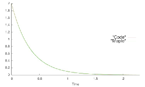
Figure 2. Computation of $\Psi(t,X)=2e^{-3t}$.

We now test the accuracy of our code by the numerical localization of a future horizon and its robustness by checking the asymptotic behaviour (IV.1). We choose different initial data and a small time step: $0.00015$. We present our results for two initial data at time $t^{\star}$ denoted $Init_{1}$ and $Init_{2}$, of the form:

(IV.4) $$u_{0}(X)=100e^{\frac{d^{2}(X,0)}{d^{2}(X,0)-R_{0}^{2}}},\;\;\mbox{for}\;d(X,0)<R_{0},\;\mbox{and}\;u_{0}(X)=0,\;\;\mbox{for}\;d(X,0)\geq R_{0}.$$

For $Init_{1}$ we have $R_{0}=0.1$ and for $Init_{2}$, $R_{0}=0.05$. In order to simplify we choose $\partial_{t}u(t^{\star},.)=u_{1}(.)=0$. Figure (3) and figure (4) present the initial data and the limit state on the slice $z=0$ of $\mathcal{F}_{v}$ observed at time $t_{obs}>t^{*}$ that we choose large enough in order to that the asymptotic state is reached. Figure (5) shows the time evolution of the solution associated to $Init_{1}$ for some points $P$ of $\mathcal{F}_{v}$ pointed out in figure (3), and figure (6) shows the time evolution of the solution associated to $Init_{2}$ for some point $PP$ of $\mathcal{F}_{v}$ pointed out in figure (4). In the following, $M0$ denotes a node of the mesh that is the closest to the center $0$ of $\mathcal{F}_{v}$.

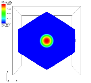
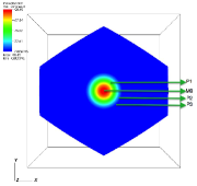
Figure 3. Solution for $Init_{1}$, on the left at $t^{\star}=3.5$, on the right at $t_{obs}=28.7$.

There is a future horizon and $R_{h}=\sin\left(\arcsin 0.1+e^{-3.5}\right)\simeq 0.13$.

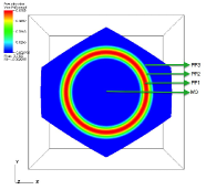
Figure 4. Solution for $Init_{2}$, on the left at $t^{\star}=1.5$, on the right at $t_{obs}=19.7$.

In this case we do have $R_{h}=\sin\left(\arcsin 0.05+e^{-1.5}\right)\simeq 0.27$.

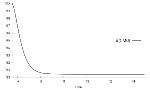
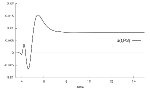
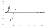
Figure 5. The solution $u(t,X)$ at M0, P1, P2, P3 with $Init_{1}$ and $t^{\star}=3.5$.

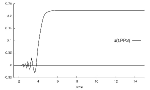
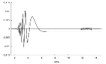
Figure 6. The solution $u(t,X)$ at M0, PP1, PP2, PP3 with $Init_{2}$ and $t^{\star}=1.5$.

Point	$d(0_{{\mathbb{R}}^{3}},M)$	$u(15,M)$
M0	$\quad 0.00008\quad$	90.45
P1	$\quad 0.064<R\quad$	37.47
P2	$\quad 0.126\leq R_{h}\quad$	0.008
P3	$\quad 0.131\simeq R_{h}\quad$	0.0016

Table 1. $Init_{1}$ and $t^{\star}=3.5$, $R_{h}\simeq 0.1299$

Point	$d(0_{{\mathbb{R}}^{3}},M)$	$u(15,M)$
$M0$	$0.00008<R$	0.0032
$PP1$	$R<0.218<R_{h}$	0.51
$PP2$	$R<0.245<R_{h}$	0.22
$PP3$	$R<0.270\simeq R_{h}$	-0.0017

Table 2. $Init_{2}$ and $t^{\star}=1.5$, $R_{h}\simeq 0.2697$

It clearly appears that a limit state is reached very quickly, as soon as $t=8$ in both cases. We also note the existence of a future horizon. In table (2) and table (2) we can read the distance between previous points $M(x_{M},y_{M},z_{M})$ of $\mathcal{F}_{v}$ and its center. The agreement between the value of $R_{h}$ given by equation (II.33), equation (II.32) is quite good, but it is difficult to have a precise numerical estimation of this horizon; for example P2 and P3 belong to a same tetrahedron, so the theoretical horizon passes throught this tetrahedron. For $Init_{1}$ and $t^{\star}=3.5$ it is found that outside the ball of radius $0.129$ the solution is always less than $0.01$, and outside the ball of radius $0.142$ the solution is always less than $0.001$. Knowing that the limit state reaches $90$ we conclude that the numerical estimation of $R_{h}$ is satisfactory.

For large time, the time derivative becomes smaller and smaller, so the energy continues decreasing and there is no longer evolution even to $t=30$. $E_{d}$ defined by equation (IV.3) is decreasing. For example for $Init_{2}$ and $t^{\star}=1.5$ we have obtained:

$$\begin{array}[]{|c|c||c|c||c|c||c|c||c|c|}\hline\cr\mbox{Time }t&E_{d}(t)&\mbox{Time }t&E_{d}(t)&\mbox{Time }t&E_{d}(t)&\mbox{Time }t&E_{d}(t)&\mbox{Time }t&E_{d}(t)\\ \hline\cr t^{\star}=1.5&217.16&3&0.56&4.8&1.\;10^{-3}&11&2.5\;10^{-9}&19.5&10^{-16}\\ \hline\cr\end{array}$$

The test of the asymptotic behaviour equation (III.42) is presented in figure (7) where we note that $Norm$ is rapidly decreasing until $t=10$.

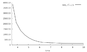
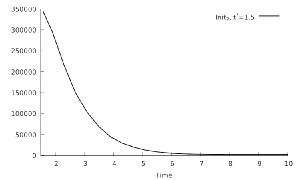
Figure 7. Validation of asymptotic behaviour equation (IV.1): $Norm$ with respect to time

We emphasize that the exponential growth of the coefficients makes the computations very difficult, and this test shows the robustness of our numerical method.

IV.2. Numerical results for $d\mathcal{S}_{4}(\mathbf{K})$.

We assume the Hubble constant is equal to $1$ hence the scale factor is $a(t)=\cosh(t)$. First we test the accuracy of our scheme in the trivial case of the constant solution $\Psi(t,X)=2$. Taking $\Psi(0,X)=2$, $\Psi(\Delta t,X)=2$ with $\Delta t=1.5\;10^{-4}$, our scheme gives a constant solution $\Psi(t,X)=2\pm 10^{-12}$ for $t\in[0,3.5]$ and the energy is around $10^{-15}$.

On the other hand we test our scheme by comparing it with two other numerical methods for computing the solution

(IV.5) $$\Psi(t,X)=A_{0}^{-}\left(\cosh t\right)^{-\frac{3}{2}}\mathrm{P}_{\frac{1}{2}}^{-\frac{3}{2}}\left(\tanh t\right).$$

In figure (8) we present the results computed by:

(i) our finite elements scheme with initial data

(IV.6) $$\Psi(0,X)=\frac{1}{2}\sqrt{\frac{\pi}{2}},\;\Psi(\Delta t,X)=\Psi(0,X)-\sqrt{\frac{2}{\pi}}\Delta t,\;\;\Delta t=1.5\;10^{-4}.$$

(ii) a Runge-Kunta scheme for the ordinary differential equation (III.18) with the same data (IV.6).

(iii) a symbolic calculation of $\left(\cosh t\right)^{-\frac{3}{2}}\mathrm{P}_{\frac{1}{2}}^{-\frac{3}{2}}\left(\tanh t\right)$ by using MAPLE.

The three curves perfectly matche and we can see only a unique graph. In fact the numerical values are the same at $\pm 5\;10^{-6}$.

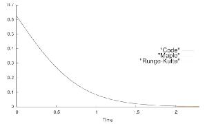
Figure 8. The black curve is the superposition of the three colored curves.

In the sequel we take initial data $Init_{2}$ and $\partial_{t}u(t^{\star},.)=0$, for various $t^{*}$. This is the initial data presented in the first picture of figure (4). First we check the accuracy of the numerical localization of a future horizon. We choose $t^{\star}=3.5$. Then $R_{h}\simeq 0.11$. Results are presented in figure (9) and figure (10). Figure (9) shows the initial data at time $t^{*}=3.5$ and at time $t_{obs}=20.08$ for which the asympotic state is reached. The pictures are on the slice $z=0$ of the dodecahedron. There is a future horizon and the support of the field is strictly included in ${\mathbf{K}}$. Figure (10) presents the time evolution of the solution at some points $MM$ of $\mathcal{F}_{v}$ depicted in figure (9). In table (4) and table (4) we can read the distance between previous points $M(x_{M},y_{M},z_{M})$ of $\mathcal{F}_{v}$ and its center, and all these numerical results are in good agreement with the theoretical results on the future horizon (II.27) and the asymptotic profile.

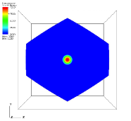
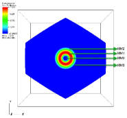
Figure 9. Solution for $Init_{2}(R_{0}=0.05)$, on the left at $t^{\star}=3.5$, on the right at $t_{obs}=20.08$.

There is a horizon and $R_{h}=\sin\left(\arcsin 0.05-2\arctan(e^{3.5})+\pi\right)\simeq 0.11$.

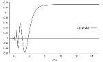
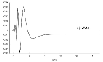
Figure 10.

Solution $u(t,X)$ with initial data $Init_{2}$ at $t^{\star}=3.5$.

As for $a(t)=e^{t}$ we see that the limit state is quickly reached: as soon as $t=9$ in both cases. $E_{d}$ defined by equation (IV.3) is decreasing as we can see for example for $Init_{2}$ and $t^{\star}=1.5$:

$$\begin{array}[]{|c|c||c|c||c|c||c|c||c|c|}\hline\cr\mbox{Time }t&E_{d}(t)&\mbox{Time }t&E_{d}(t)&\mbox{Time }t&E_{d}(t)&\mbox{Time }t&E_{d}(t)&\mbox{Time }t&E_{d}(t)\\ \hline\cr t^{\star}=1.5&4361&3.4&0.49&5&1.2\;10^{-3}&11.5&10^{-9}&19.6&9.\;10^{-17}\\ \hline\cr\end{array}$$

Point	$d(0_{{\mathbb{R}}^{3}},M)$	$u(15,M)$
M0	$\quad 0.00008\quad$	-0.0005
M1	$\quad 0.270\quad$	0.415
M2	$\quad 0.182\quad$	0.004
M3	$\quad 0.354\quad$	0.013

Table 3. $Init_{2}$ and $t^{\star}=1.5$, no horizon.

Point	$d(0_{{\mathbb{R}}^{3}},M)$	$u(15,M)$
$M0$	0.00008	-0.016
$MM1$	0.0544	7.41
$MM2$	0.1004	0.131
$MM3$	0.1055	-0.008

Table 4. $Init_{2}$ and $t^{\star}=3.5$, $R_{h}\simeq 0.11$

Finally we test the robustness of our code by the hard computation of equation (IV.1). We consider the solution with initial data given at $t^{*}=1.5$ and $t^{*}=3.5$. In all cases the quantity $Norm$ that tests equation (III.15) quickly tends to zero. On figure (11) we remark that for $t^{\star}=1.5$ $Norm$ is decreasing except when the support of the solution reaches the border of $\mathcal{F}_{v}$ at $t\simeq 2.3$ (we detail the peculiar properties of this solution below). We conclude that as for $a(t)=e^{t}$, the tests of equation (III.15) by the computation of $Norm$ prove that our numerical scheme is accurate and robust.

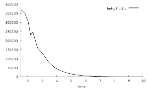
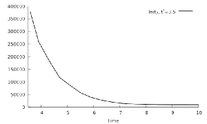
Figure 11. Validation of equation (IV.1) : $Norm$ with respect to time

We end this part by the most interesting case: we present two solutions with “the circles-in-the-sky”. Firstly we consider the previous solution with data $\Psi(t^{*},.)$ described by $Init_{2}$ and $\partial_{t}\Psi(t^{\star},.)=0$ given at $t^{\star}=1.5$. Then $R_{h}$ is equal to $\sin\left(\arcsin 0.05-2\arctan(e^{1.5})+\pi\right)\sim 0.469$ which is greater than $\sin(d_{max})\simeq 0.378$. Therefore the support of the solution is the whole $\mathcal{F}_{v}$ for $t$ large enough and the constraint (II.31) is fulfilled: we shall be able to see multiple copies of the asymptotic profile.

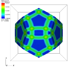
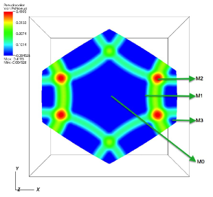
Figure 12. Solution observed at $t_{obs}=15.06$ for $Init_{2}$ and $t^{\star}=1.5$. Left: on the boundary of the dodecahedron. Right: on the slice at $z=0$.

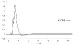
Figure 13.

Solution $u(t,X)$ with initial data $Init_{2}$ at $t^{\star}=1.5$.

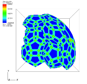
Figure 14.

Pull-back of the solution at $t_{obs}=15.06$ in a part of the universal covering $\mathcal{S}^{3}$ of $\mathbf{K}$.

Figure (12) shows the solution at time $t_{obs}=15.06$ on the boundary of the dodecahedron, $\partial\mathcal{F}_{v}$, and in its interior, on the slice $z=0$. In fact, at this time the asymptotic state is reached. We can see this fast convergence on figure (13) that shows the time evolution of the solution at some points $M$ of $\mathcal{F}_{v}$ depicted in figure (12). Since the whole universe is included inside the horizon sphere, it is interesting to present the pull-back of the solution in the universal covering ${\mathcal{S}}^{3}$ of $\mathbf{K}$. Figure (14) shows the solution on a partial tiling of the unit ball $\mathcal{B}^{\prime}$ (see figure (1) and the explanations after formula equation (II.5).

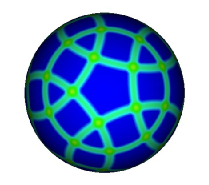
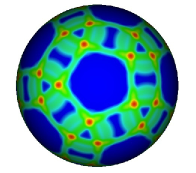
Figure 15.

Deep skies: on the left $\chi=\arcsin(0.5)\simeq 0.523$, on the right $\chi=\arcsin(0.6)\simeq 0.643$.

We now show the application of our numerical method to the determination of the temperature fluctuation in the deep sky. We consider an observer located at time $t_{0}$ at the centre of the Poincaré dodecahedron, $x=y=z=0$, that corresponds to the north pole of $\mathcal{S}^{3}$, defined by $(x^{0},x^{1},x^{2},x^{3})=(1,0,0,0)$, or in spherical coordinates, $\chi=0$. We assume the initial pertubation of the metric is given by $Init_{2}$ at $t^{*}=1.5$ and $t_{0}$ is large enough for the asymptotic state to be reached. Then according to the Sachs-Wolfe formula equation (I.4), the temperature fluctuation seen by this observer in the direction $(\theta,\varphi)\in\mathcal{S}^{2}$ is given by

$$\frac{\delta T(\theta,\varphi)}{T}\simeq\frac{1}{3}\Psi_{\infty}(\chi,\theta,\varphi),$$

where the angle $\chi$ is determined by $\chi=\eta_{0}-\eta_{ls}$ that is the conformal time between the time of recombination $t_{ls}$ and $t_{0}$ ($t^{*}<t_{ls}<t_{0}$). Its value is given by equation (II.32),

$$\chi=2\arctan\left(e^{t_{0}}\right)-2\arctan\left(e^{t_{ls}}\right),$$

and the sky seen by the observer corresponds to the horizon sphere centered at the origin, included in $\mathcal{B}^{\prime}$, with the radius $R_{t_{ls},t_{0}}=\sin\chi$. Figure (15) shows the deep sky for $R_{t_{ls},t_{0}}=0.5$ and $R_{t_{ls},t_{0}}=0.6$ (we recall that by equation (II.22) the radius of the smallest ball containing $\mathbf{K}$ is $R_{max}\simeq 0.378$). We remark that the initial perturbation of the metric leads to a temperature fluctuation that shows spherical correlations along six pairs of antipodal matched circles (the famous circles-in-the-sky) that are a signature of a complex topology with a positive curvature. In contrast, a complex topology and a negative curvature lead to chaotic temperature fluctuations [4].

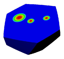
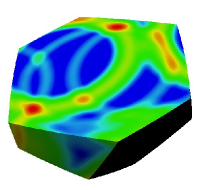
Figure 16.

Solution for $Init_{3}$ on the cut $10x+5y-15z=0$: on the left at $t^{*}=2$, on the right, the asymptotic profile.

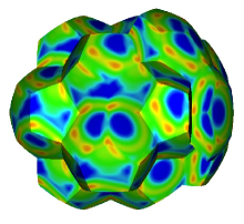
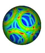
Figure 17.

On the left the asymptotic state in a part of the universal covering $\mathcal{S}^{3}$ of $\mathbf{K}$ around $(1,0,0,0)$. On the right the deep sky for $\chi=\arcsin(0.55)\simeq 0.582$.

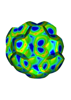
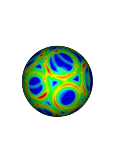
Figure 18.

On the left the asymptotic state in a part of the universal covering $\mathcal{S}^{3}$ of $\mathbf{K}$. On the right the deep sky for $\chi=\pi-\arcsin(0.6)\simeq 2.498$.

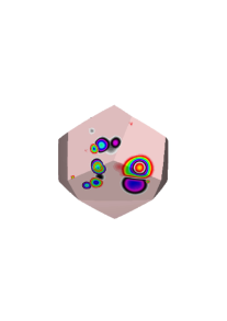
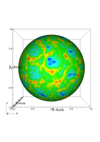
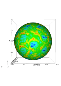
Figure 19.

An initial random fluctuation and two antipodal views of the deep sky for $\chi=\pi/2$.

We now present a more complex solution associated to an initial data $u(t^{*},.)=Init_{3}$, $\partial_{t}u(t^{*},.)=0$ given at time $t^{*}=2$. $Init_{3}$ is composed of $Init_{2}$ to which we have added two another fields of the same type (see (IV.4)): one with $X_{0}=(0.1,0.1,0.1)$ and $R_{0}=0.1$, the other with $X_{0}=(-0.15,0,-0.1)$ and $R_{0}=0.05$. We take $A_{0}=100$ again. Figure 16 shows $Init_{3}$ and the asymptotic profile on the two-plane $10x+5y-15z=0$. The left figure 17 shows the pull-back of $\Psi_{\infty}$ on a part of the universal covering $\mathcal{S}^{3}$ of $\mathbf{K}$, included in $\mathcal{B}^{\prime}$ (see (II.6)), composed by $\mathcal{F}_{v}$, $p\left(g_{i}(\mathcal{F})\right)$ with $i=1,...,12$, $p\left(g_{i}\circ g_{6}(\mathcal{F})\right)$ with $i=1,...,5$, $p\left(g_{i}\circ g_{3}(\mathcal{F})\right)$ with $i=1,2,4,5,6$ (see (II.9) and the Appendix). On the right the deep sky for $\chi\simeq 0.582$ is depicted. Similarly Figure 18 presents the case of a large conformal time. On the left, the part of the universal covering of $\mathbf{K}$ is included in the second unit ball $\mathcal{B}^{\prime\prime}$ associated to $\chi\in[\frac{\pi}{2},\pi]$. This set is composed by $p(-\mathbf{1}\mathcal{F})$, $p\left(g_{i}(-\mathbf{1}\mathcal{F})\right)$ with $i=1,...,12$, $p\left(g_{i}\circ g_{6}(-\mathbf{1}\mathcal{F})\right)$ with $i=1,...,5$, $p\left(g_{i}\circ g_{3}(-\mathbf{1}\mathcal{F})\right)$ with $i=1,2,4,5,6$. On the right the deep sky for $\chi\simeq 2,498$. We note the correlations along six pairs of circles again.

We achieve this part with the more realistic case of a random initial fluctuation ${\it Init_{4}}$ composed with 100 localized fluctuations of type (IV.4). The radius $R_{0}$, the centers $X_{0}$, and the amplitudes $A_{0}$ are randomly choosen such that $-100\leq A_{0}\leq 100$, $R_{0}\leq 0.1$. The left figure 19 shows ${\it Init_{4}}$ on a cut of the dodecahedron along three planes. We compute the solution for $u(t^{*},.)={\it Init_{4}}$, $\partial_{t}u(t^{*},.)=0$ given at time $t^{*}=2$. The right figure 19 presents two antipodal views of the deep sky for $\chi=\pi/2$. We can guess the correlations of the fluctuations along six pairs of matched antipodal circles.

V. Conclusion

In this paper we have considered models of dynamical spacetimes for which the spatial section is the Poincaré dodecahedron. We have solved the Cauchy problem for the D’Alembertian and expressed the initial value problem in terms of variational formulation put on the fundamental domain. We have established the existence of an asymptotic state $\Psi_{\infty}$ at the time infinity for the finite energy waves:

$$\Psi_{\infty}:=\lim_{t\rightarrow\infty}\Psi(t).$$

If $\Psi$ is the perturbation of the metric, this state describes the temperature fluctuations in the deep sky thanks to the (ordinary) Sachs-Wolfe formula

$$\frac{\delta T}{T}\simeq\frac{1}{3}\Psi_{\infty}.$$

We have obtained the analytic expression of this limit state for two important cases of accelerating universes associated to the scale factors $H^{-1}\cosh(Ht)$ and $e^{t}$. It turns out that $\Psi_{\infty}$ is given by a pseudodifferential operator acting on the inital data of the perturbation, $(\Psi(0),\partial_{t}\Psi(0))$ that is not convenient for the computation. Therefore we have performed a numerical method for solving the time evolution problem. We also emphasize that this step is necessary if we want to use the integrated Sachs-Wolfe formula involving $\Psi(t)$ for any time $t$ since the last time of recombination. We employ the ${\mathbb{P}}_{2}$ type finite elements for the sake of accuracy. The numerical experiments show a good agreement with the theoretical results on the asymptotic behaviours. That proves the robustness and the accuracy of our method as well as its efficiency to compute the deep sky. Its drawback is the lenght of the computation, usually we need one week to go from $t$ to $t+1.2$ and this time of calculation would explode for a very refined mesh. We can hope to be able to use a parallel computing together with a domain decomposition on a significantly refined mesh. Then we shall be able to treat the heavy computations associated to random initial data and the integrated Sachs-Wolfe formula.

Appendix

This appendix is devoted to a brief description of $\mathcal{F}$ and $\mathcal{F}_{v}$. For more details on the construction of these domains we refer to [5].

First of all we recall that the binary icosahedral group $\mathcal{I}^{*}$ is generated by two isometries $s$ and $\gamma$. Denoting by $\sigma=(1+\sqrt{5})/2$ the golden number we have:

$$\mathcal{I}^{*} =\left<s,\gamma\;|\;(s\gamma)^{2}=s^{3}=\gamma^{5}\right>$$

$$=\left\{\pm\mathbf{1},\pm\mathbf{i},\pm\mathbf{j},\pm\mathbf{k},\frac{1}{2}(\pm\mathbf{1}\pm\mathbf{i}\pm\mathbf{j}\pm\mathbf{k}),\frac{1}{2}(0\mathbf{1}\pm\mathbf{i}\pm\frac{1}{\sigma}\mathbf{j}\pm\sigma\mathbf{k})\;(with\;even\;permutations)\right\}.$$

where $\{\mathbf{1},\mathbf{i},\mathbf{j},\mathbf{k\}}$ are the four basic quaternions of the set ${\mathbb{H}}$ of all quaternions. Twelve Cliffort translations $g_{i}$ belonging to $\mathcal{I}^{*}$ are involved in the construction of $\mathcal{F}$:

$$\ g_{1}:=\frac{1}{2}\sigma\mathbf{1}+\frac{1}{2}\frac{1}{\sigma}\mathbf{i}+\frac{1}{2}\mathbf{j},\quad \;g_{2}:=\frac{1}{2}\sigma\mathbf{1}+\frac{1}{2}\mathbf{i}-\frac{1}{2}\frac{1}{\sigma}\mathbf{k},\quad \;g_{3}:=\frac{1}{2}\sigma\mathbf{1}+\frac{1}{2}\frac{1}{\sigma}\mathbf{j}-\frac{1}{2}\mathbf{k},$$

$$\ g_{4}:=\frac{1}{2}\sigma\mathbf{1}-\frac{1}{2}\frac{1}{\sigma}\mathbf{i}+\frac{1}{2}\mathbf{j},\quad \;g_{5}:=\frac{1}{2}\sigma\mathbf{1}+\frac{1}{2}\frac{1}{\sigma}\mathbf{j}+\frac{1}{2}\mathbf{k},\quad \;g_{6}:=\frac{1}{2}\sigma\mathbf{1}+\frac{1}{2}\mathbf{i}+\frac{1}{2}\frac{1}{\sigma}\mathbf{k}.$$

They are such that: $\quad\forall i\in\{1,...,6\},\;g_{i}(F_{i})=F_{i+6}$ ($F_{i}$ denote faces of $\mathcal{F}$). The inverses of these six first translations are the six other translations:

$$\ g_{7}:=(g_{1})^{-1}=\frac{1}{2}\sigma\mathbf{1}-\frac{1}{2}\frac{1}{\sigma}\mathbf{i}-\frac{1}{2}\mathbf{j}, \;g_{8}:=(g_{2})^{-1}=\frac{1}{2}\sigma\mathbf{1}-\frac{1}{2}\mathbf{i}+\frac{1}{2}\frac{1}{\sigma}\mathbf{k},$$

$$\ g_{9}:=(g_{3})^{-1}=\frac{1}{2}\sigma\mathbf{1}-\frac{1}{2}\frac{1}{\sigma}\mathbf{j}+\frac{1}{2}\mathbf{k}, \;g_{10}:=(g_{4})^{-1}=\frac{1}{2}\sigma\mathbf{1}+\frac{1}{2}\frac{1}{\sigma}\mathbf{i}-\frac{1}{2}\mathbf{j},$$

$$\ g_{11}:=(g_{5})^{-1}=\frac{1}{2}\sigma\mathbf{1}-\frac{1}{2}\frac{1}{\sigma}\mathbf{j}-\frac{1}{2}\mathbf{k}, \;g_{12}:=(g_{6})^{-1}=\frac{1}{2}\sigma\mathbf{1}-\frac{1}{2}\mathbf{i}-\frac{1}{2}\frac{1}{\sigma}\mathbf{k}.$$

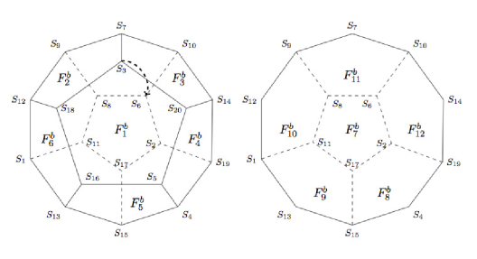
Figure 20. Diagram of vertices $S_{i}$, edges and faces of $\mathcal{F}_{v}$.

We warn that Figure (20) is not a faithful representation of $\mathcal{F}_{v}$ as, for convenience, we have replaced the true curved faces of $\mathcal{F}_{v}$ by the plane faces $F^{b}_{i}$ that are the projection on ${\mathbb{R}}^{3}$ of the sets of all barycenters in ${\mathbb{R}}^{4}$ of the vertices $S_{i}^{1},...,S_{i}^{5}$ of the faces $F_{i}$ of $\mathcal{F}$.

1. Coordinates of the vertices $S_{i}$ of $\mathcal{F}$:

   $$\begin{array}[]{ll}S_{1}=\frac{1}{2\sqrt{2}}\left(\sigma^{2},-\frac{1}{\sigma},\frac{1}{\sigma},-\frac{1}{\sigma}\right),&S_{2}=\frac{1}{2\sqrt{2}}\left(\sigma^{2},1,\frac{1}{\sigma^{2}},0\right),\\ S_{3}=\frac{1}{2\sqrt{2}}\left(\sigma^{2},-\frac{1}{\sigma},-\frac{1}{\sigma},\frac{1}{\sigma}\right),&S_{4}=\frac{1}{2\sqrt{2}}\left(\sigma^{2},\frac{1}{\sigma},-\frac{1}{\sigma},-\frac{1}{\sigma}\right),\\ S_{5}=\frac{1}{2\sqrt{2}}\left(\sigma^{2},0,-1,-\frac{1}{\sigma^{2}}\right),&S_{6}=\frac{1}{2\sqrt{2}}\left(\sigma^{2},\frac{1}{\sigma},\frac{1}{\sigma},\frac{1}{\sigma}\right),\\ S_{7}=\frac{1}{2\sqrt{2}}\left(\sigma^{2},-\frac{1}{\sigma^{2}},0,1\right),&S_{8}=\frac{1}{2\sqrt{2}}\left(\sigma^{2},0,1,\frac{1}{\sigma^{2}}\right),\\ S_{9}=\frac{1}{2\sqrt{2}}\left(\sigma^{2},-\frac{1}{\sigma},\frac{1}{\sigma},\frac{1}{\sigma}\right),&S_{10}=\frac{1}{2\sqrt{2}}\left(\sigma^{2},\frac{1}{\sigma^{2}},0,1\right),\\ S_{11}=\frac{1}{2\sqrt{2}}\left(\sigma^{2},0,1,-\frac{1}{\sigma^{2}}\right),&S_{12}=\frac{1}{2\sqrt{2}}\left(\sigma^{2},-1,\frac{1}{\sigma^{2}},0\right),\\ S_{13}=\frac{1}{2\sqrt{2}}\left(\sigma^{2},-\frac{1}{\sigma^{2}},0,-1\right),&S_{14}=\frac{1}{2\sqrt{2}}\left(\sigma^{2},\frac{1}{\sigma},-\frac{1}{\sigma},\frac{1}{\sigma}\right),\\ S_{15}=\frac{1}{2\sqrt{2}}\left(\sigma^{2},\frac{1}{\sigma^{2}},0,-1\right),&S_{16}=\frac{1}{2\sqrt{2}}\left(\sigma^{2},-\frac{1}{\sigma},-\frac{1}{\sigma},-\frac{1}{\sigma}\right),\\ S_{17}=\frac{1}{2\sqrt{2}}\left(\sigma^{2},\frac{1}{\sigma},\frac{1}{\sigma},-\frac{1}{\sigma}\right),&S_{18}=\frac{1}{2\sqrt{2}}\left(\sigma^{2},-1,-\frac{1}{\sigma^{2}},0\right),\\ S_{19}=\frac{1}{2\sqrt{2}}\left(\sigma^{2},1,-\frac{1}{\sigma^{2}},0\right),&S_{20}=\frac{1}{2\sqrt{2}}\left(\sigma^{2},0,-1,\frac{1}{\sigma^{2}}\right).\end{array}$$

2. Images by the Clifford translation $g_{i}$ of the face $F_{i}$ of $\mathcal{F}$ and of its edges.
   $g_{1}$ maps $F_{1}$ to $F_{7}$, and we have for the vertices and the edges:
   $g_{1}(S_{3})=S_{6},\quad g_{1}(S_{18})=S_{8},\quad g_{1}(S_{16})=S_{11},\quad g_{1}(S_{5})=S_{17},\quad g_{1}(S_{20})=S_{2}$,

   $g_{1}(\wideparen{S_{3}S_{18}})=\wideparen{S_{6}S_{8}},\;g_{1}(\wideparen{S_{18}S_{16}})=\wideparen{S_{8}S_{11}},\;g_{1}(\wideparen{S_{16}S_{5}})=\wideparen{S_{11}S_{17}},\;g_{1}(\wideparen{S_{5}S_{20}})=\wideparen{S_{17}S_{2}},$

   $g_{1}(\wideparen{S_{20}S_{3}})=\wideparen{S_{2}S_{6}}$.
   

   $g_{2}$ maps $F_{2}$ to $F_{8}$, and we have for the vertices and the edges:
   $g_{2}(S_{18})=S_{15},\quad g_{2}(S_{12})=S_{17},\quad g_{2}(S_{9})=S_{2},\quad g_{2}(S_{7})=S_{19},\quad g_{2}(S_{3})=S_{4}$,

   $g_{2}(\wideparen{S_{18}S_{12}})=\wideparen{S_{15}S_{17}},\;g_{2}(\wideparen{S_{17}S_{2}})=\wideparen{S_{8}S_{11}},\;g_{2}(\wideparen{S_{9}S_{7}})=\wideparen{S_{2}S_{19}},\;g_{2}(\wideparen{S_{7}S_{3}})=\wideparen{S_{19}S_{4}},$

   $g_{2}(\wideparen{S_{3}S_{18}})=\wideparen{S_{4}S_{15}}$.
   

   $g_{3}$ maps $F_{3}$ to $F_{9}$, and we have for the vertices and the edges:
   $g_{3}(S_{3})=S_{1},\quad g_{3}(S_{7})=S_{11},\quad g_{3}(S_{10})=S_{17},\quad g_{3}(S_{14})=S_{15},\quad g_{3}(S_{20})=S_{13}$,

   $g_{3}(\wideparen{S_{3}S_{7}})=\wideparen{S_{1}S_{11}},\;g_{3}(\wideparen{S_{7}S_{10}})=\wideparen{S_{11}S_{17}},\;g_{3}(\wideparen{S_{10}S_{14}})=\wideparen{S_{17}S_{15}},$
   $g_{3}(\wideparen{S_{14}S_{20}})=\wideparen{S_{15}S_{13}},\;g_{3}(\wideparen{S_{20}S_{3}})=\wideparen{S_{13}S_{1}}$.
   

   $g_{4}$ maps $F_{4}$ to $F_{10}$, and we have for the vertices and the edges:
   $g_{4}(S_{20})=S_{9},\quad g_{4}(S_{14})=S_{8},\quad g_{4}(S_{19})=S_{11},\quad g_{4}(S_{4})=S_{1},\quad g_{4}(S_{5})=S_{12}$,

   $g_{4}(\wideparen{S_{20}S_{14}})=\wideparen{S_{9}S_{8}},\;g_{4}(\wideparen{S_{14}S_{19}})=\wideparen{S_{8}S_{11}},\;g_{4}(\wideparen{S_{19}S_{4}})=\wideparen{S_{11}S_{1}},\;g_{4}(\wideparen{S_{4}S_{5}})=\wideparen{S_{1}S_{12}},$

   $g_{4}(\wideparen{S_{5}S_{20}})=\wideparen{S_{12}S_{9}}$.
   

   $g_{5}$ maps $F_{5}$ to $F_{11}$, and we have for the vertices and the edges:
   $g_{5}(S_{5})=S_{10},\quad g_{5}(S_{4})=S_{6},\quad g_{5}(S_{15})=S_{8},\quad g_{5}(S_{13})=S_{9},\quad g_{5}(S_{16})=S_{7}$,

   $g_{5}(\wideparen{S_{5}S_{4}})=\wideparen{S_{10}S_{6}},\;g_{5}(\wideparen{S_{4}S_{15}})=\wideparen{S_{6}S_{8}},\;g_{5}(\wideparen{S_{15}S_{13}})=\wideparen{S_{8}S_{9}},\;g_{5}(\wideparen{S_{13}S_{16}})=\wideparen{S_{9}S_{7}},$

   $g_{5}(\wideparen{S_{16}S_{5}})=\wideparen{S_{7}S_{10}}.$
   

   $g_{6}$ maps $F_{6}$ to $F_{12}$, and we have for the vertices and the edges:
   $g_{6}(S_{16})=S_{19},\quad g_{6}(S_{13})=S_{2},\quad g_{6}(S_{1})=S_{6},\quad g_{6}(S_{12})=S_{10},\quad g_{6}(S_{18})=S_{14}$,

   $g_{6}(\wideparen{S_{16}S_{13}})=\wideparen{S_{19}S_{2}},\;g_{6}(\wideparen{S_{13}S_{1}})=\wideparen{S_{2}S_{6}},\;g_{6}(\wideparen{S_{1}S_{12}})=\wideparen{S_{6}S_{10}},$
   $g_{6}(\wideparen{S_{12}S_{18}})=\wideparen{S_{10}S_{14}},\;g_{6}(\wideparen{S_{18}S_{16}})=\wideparen{S_{14}S_{19}}$.

Then we define the equivalence classes on $\mathcal{F}$ by:

$$\begin{array}[]{l}q\in\stackrel{{\scriptstyle\circ}}{{\mathcal{F}}}\quad\Rightarrow\dot{q}=\{q\},\\ \exists(i,j,k),\;q\in F_{i}\cap F_{j}\cap F_{k}\quad\Rightarrow\dot{q}=\{q,g_{i}(q),g_{j}(q),g_{k}(q)\},\\ (\exists(i,j),\;q\in F_{i}\cap F_{j})\quad and\quad(\forall k\neq i,\;j,\;\;q\notin F_{k})\quad\Rightarrow\dot{q}=\{q,g_{i}(q),g_{j}(q)\},\\ (\exists i,\;q\in F_{i})\quad and\quad(\forall j\neq i,\;q\notin F_{j})\quad\Rightarrow\dot{q}=\{q,g_{i}(q)\}.\end{array}$$

Here the integers $i,j,k$ belong to $\{1,...,12\}$, and $F_{i}$ denotes a face of $\mathcal{F}$.

References

- [1] R. Aurich, S. Lustig, F. Steiner. CMB anisotropy of the Poincaré dodecahedron. Class. Quantum Grav., 22: 2061–2083, 2005 (arXiv:astro-ph/0412569).
- [2] R. Aurich, S. Lustig, F. Steiner. The circles-in-the-sky signature for three spherical universes. Mon. Not. Roy. Astron. Soc., 369: 240–248, 2006 (arXiv:astro-ph/0510847).
- [3] Al. Bachelot. On the Klein-Gordon equation near a De Sitter brane in an Anti-de Sitter bulk. J. Math. Pures Appl., 105, 165–197, 2016 (arXiv:1402.1071).
- [4] Ag. Bachelot-Motet. Wave computation on the hyperbolic double doughnut. J. Comp. Math., 28-6: 790–806, 2010 (arXiv:0902.1249).
- [5] Ag. Bachelot-Motet. Wave computation on the Poincaré dodecahedral space. Class. Quantum Grav., 30-23:235010, 2013 (arXiv:math-ph/1302.6537v2).
- [6] M. Bellon. Elements of dodecahedral topology. Class. Quantum Grav., 23: 7029–7043, 2006 (arXiv:astro-ph/0602076).
- [7] C. L. Bennett, D. Larson, J. L. Weiland, N. Jarosik, G. Hinshaw, N. Odegard, K. M. Smith, R. S. Hill, B. Gold, M. Halpern, E. Komatsu, M. R. Nolta, L. Page, D. N. Spergel, E. Wollack, J. Dunkley, A. Kogut, M. Limon, S. S. Meyer, G. S. Tucker, E. L. Wright. Nine-Year Wilkinson Microwave Anisotropy Probe (WMAP) Observations: Final Maps and Results. Astrophys. J. Suppl. , 208-2, 2013 (arXiv:astro-ph/1212.5225v3).
- [8] S. Caillerie, M. Lachièze-Rey, J.-P. Luminet, R. Lehoucq, A. Riazuelo, J. Weeks. A new analysis of the Poincaré dodecahedral space model. Astron. Astrophys., 476-2: 691–696, 2007 (arXiv:astro-ph/0705.0217v2).
- [9] Y. Choquet-Bruhat. General Relativity and the Einstein Equations. Oxford University Press, 2009.
- [10] S. H. Christiansen. Foundations of finite element methods for wave equation of Maxwell type. Springer, Applied Wave Mathematics, 335, 2009.
- [11] N. Cornish , D. Spergel, G. Starkman. Circles in the sky: finding topology with the microwave background radiation. Class. Quantum Grav., 15: 2657–2670, 1998 (arXiv:astro-ph/9801212).
- [12] W. Czaja, Z. A. Golda, A. Woszczyna. The acoustic wave equation in the expanding Universe: Sachs-Wolfe Theorem. Mathematica J., 13: 8pp., 2011 (arXiv:0902.0239).
- [13] R. Dautray, J.-P. Lions, Mathematical Analysis and Numerical Methods for Science and Technology, Volume 5 Evolution Problems I. Springer-Verlag, 2000.
- [14] E. Gaussmann, R. Lehoucq, J.-P. Luminet, J.-Ph. Uzan, J. Weeks. Topological lensing in spherical spaces. Class. Quantum Grav., 18: 5155–5186, 2001 (arXiv:gr-qc/0106033v1).
- [15] Z. A. Golda, A. Woszczyna. A field theory approach to cosmological density perturbations. Phys. Lett., A 310: 357–362, 2003 (arXiv:gr-qc/0302091).
- [16] W. El. Hanafy, G. L. Nashed. Reconstruction of -gravity in the absence of matter. DOI=”10.1007/s10509-016-2786-0”, Astrophys. Space Sci., 2016 (arXiv:hep-th/1410.2467v3).
- [17] A. Ikeda. On the spectrum of homogeneous spherical space forms. Kodai Math. J., 18: 57, 1995.
- [18] P. Keast. url: http://nines.cs.kuleuven.be/research/ecf/mtables.htmlnines.cs.kuleuven.be Moderate-degree tetrahedral quadrature formulae. Comput. Methods Appl. Mech. Engrg., 55, 339–348, 1986.
- [19] S. Klainerman, P. Sarnak. Explicit solutions of on the Friedmann-Robertson-Walker space-times. Ann. Inst. Henri Poincaré, A 35: 253–257, 1981.
- [20] M. Lachièze-Rey. Eigenmodes of dodecahedral space. Class. Quantum Grav., 21:2455–2464, 2004.
- [21] R. Lehoucq, J. Weeks, J.-Ph. Uzan, E. Gaussmann,J.-P. Luminet. Eigenmodes of three-dimensional spherical spaces and their application to cosmology. Class. Quantum Grav., 19:4683–4708, 2002 (arXiv:gr-qc/0205009v1).
- [22] J. Leray. Hyperbolic differential equations, Princeton University Press, 1953.
- [23] J.-P. Luminet, B. F. Roukema. Topology of the Universe: Theory and Observation, Theoretical and Observational Cosmology, 541, 117–156, 1999 (arXiv:astro-ph/9901364v3).
- [24] J.-P. Luminet. The shape and topology of the universe, 2008, (arXiv:astro-ph/0802.2236).
- [25] J.-P. Luminet, J. Weeks, A. Riazuelo, R. Lehoucq, J.-Ph. Uzan. Dodecahedral space topology as an explanation for weak wide-angle temperature correlations in the cosmic microwave background. Letters to nature, 425, 593:595, 2003 (arXiv:astro-ph/0310253v1).
- [26] B. McInnes. APS Instability and the Topology of the Brane-World. Phys. Lett. B 593:10-16, 2004 (arXiv: hep-th/0401035v4).
- [27] B. Mota, M. J. Rebouças, R. Tavakol. Circles-in-the-sky searches and observable cosmic topology in the inflationary limit. Phys. Rev. D, 78: 083521, 2008 (arXiv:0808.1572).
- [28] V. F. Mukhanov, H. A. Feldman, R. H. Brandenberger. Theory of cosmological perturbations. Phys. Rep., 215: 203–333, 1992.
- [29] F. W. J. Olver, D. W. Lozier, R. F. Boisvert, and C. W. Clark. url: http://dlmf.nist.gov/NIST Digital Library of Mathematical Functions Print version: Cambridge University Press, New York, NY, 2010.
- [30] B. F. Roukema, T. A. Kazimierczak. The size of the Universe according to the Poincaré dodecahedral space hypothesis. Astronomy and Astrophysics 533, A11, 2011 (arXiv:astro-ph/1106.0727v2).
- [31] P. Scott. The geometries of 3-manifolds. Bull. London. Math. Soc., 15:401-487, 1983.
- [32] H. Tanabe. Equations of Evolution. Monographs and Studies in Mathematics, 6, 1979.
- [33] A.Vasy. The wave equation on asymptotically de Sitter-like spaces. Adv. Math. 223, 49–97, 2010 (arXiv:math-ph/0706.3669v1).
- [34] C. Weber, H. Seifert. Die beiden Dodekaederräume. Math. Z., 37:237-253, 1933.
- [35] J. Weeks. Reconstructing the global topology of the universe from the cosmic microwave background. Class. Quantum Grav., 15: 2599-2604, 1998 (arXiv:astro-ph/9802012v1).
- [36] J. Weeks. The Poincaré dodecahedral space and the mystery of the missing fluctuations. Notices of the AMS, 51-6: 610-619, 2004.
- [37] J. A. Wolf. Spaces of Constant Curvature. 5th edn (Boston, MA: Publish or Perish), 1967.