Randomized Prediction Games for
Adversarial Machine Learning

Abstract

In spam and malware detection, attackers exploit randomization to obfuscate malicious data and increase their chances of evading detection at test time; e.g., malware code is typically obfuscated using random strings or byte sequences to hide known exploits. Interestingly, randomization has also been proposed to improve security of learning algorithms against evasion attacks, as it results in hiding information about the classifier to the attacker. Recent work has proposed game-theoretical formulations to learn secure classifiers, by simulating different evasion attacks and modifying the classification function accordingly. However, both the classification function and the simulated data manipulations have been modeled in a deterministic manner, without accounting for any form of randomization. In this work, we overcome this limitation by proposing a randomized prediction game, namely, a non-cooperative game-theoretic formulation in which the classifier and the attacker make randomized strategy selections according to some probability distribution defined over the respective strategy set. We show that our approach allows one to improve the trade-off between attack detection and false alarms with respect to state-of-the-art secure classifiers, even against attacks that are different from those hypothesized during design, on application examples including handwritten digit recognition, spam and malware detection.

I Introduction

Machine-learning algorithms have been increasingly adopted in adversarial settings like spam, malware and intrusion detection. However, such algorithms are not designed to operate against intelligent and adaptive attackers, thus making them inherently vulnerable to carefully-crafted attacks. Evaluating security of machine learning against such attacks and devising suitable countermeasures, are two among the main open issues under investigation in the field of adversarial machine learning [1, 2, 3, 4, 5, 6, 7, 8, 9, 10, 11]. In this work we focus on the issue of designing secure classification algorithms against evasion attacks, i.e., attacks in which malicious samples are manipulated at test time to evade detection. This is a typical setting, e.g., in spam filtering, where spammers manipulate the content of spam emails to get them past the anti-spam filters [12, 2, 1, 13, 14], or in malware detection, where hackers obfuscate malicious software (malware, for short) to evade detection of either known or zero-day exploits [15, 16, 8, 9]. Although out of the scope of this work, it is worth mentioning here another pertinent attack scenario, referred to as classifier poisoning. Under this setting, the attacker can manipulate the training data to mislead classifier learning and cause a denial of service; e.g., by increasing the number of misclassified samples [17, 18, 6, 7, 19, 20].

To date, several authors have addressed the problem of designing secure learning algorithms to mitigate the impact of evasion attacks [1, 21, 22, 23, 6, 10, 24, 11, 25, 26, 27] (see Sect. VII for further details). The underlying rationale of such approaches is to learn a classification function that accounts for potential malicious data manipulations at test time. To this end, the interactions between the classifier and the attacker are modeled as a game in which the attacker manipulates data to evade detection, while the classification function is modified to classify them correctly. This essentially amounts to incorporating knowledge of the attack strategy into the learning algorithm. However, both the classification function and the simulated data manipulations have been modeled in a deterministic manner, without accounting for any form of randomization.

Randomization is often used by attackers to increase their chances of evading detection, e.g., malware code is typically obfuscated using random strings or byte sequences to hide known exploits, and spam often contains bogus text randomly taken from English dictionaries to reduce the “spamminess” of the overall message. Surprisingly, randomization has also been proposed to improve classifier security against evasion attacks [28, 3, 6]. In particular, it has been shown that randomizing the learning algorithm may effectively hide information about the classification function to the attacker, requiring her to select a less effective attack (manipulation) strategy. In practice, the fact that the adversary may not know the classification function exactly (i.e., in a deterministic sense) decreases her (expected) payoff on each attack sample. This means that, to achieve the same expected evasion rate attained in the deterministic case, the attacker has to increase the number of modifications made to the attack samples [28].

Motivated by the aforementioned facts, in this work we generalize static prediction games, i.e., the game-theoretical formulation proposed by Brückner et al. [10, 11], to account for randomized classifiers and data manipulation strategies. For this reason, we refer to our game as a randomized prediction game. A randomize prediction game is a non-cooperative game between a randomized learner and a randomized attacker (also called data generator), where the player’s strategies are replaced with probability distributions defined over the respective strategy sets. Our goal is twofold. We do not only aim to assess whether randomization helps achieving a better trade-off in terms of false alarms and attack detection (with respect to state-of-the-art secure classifiers), but also whether our approach remains more secure against attacks that are different from those hypothesized during design. In fact, given that our game considers randomized players, it is reasonable to expect that it may be more robust to potential deviations from its original hypotheses about the players’ strategies.

The paper is structured as follows. Randomized prediction games are presented in Sect. II, where sufficient conditions for the existence and uniqueness of a Nash equilibrium in these games are also given. In Sect. III we focus on a specific game instance involving a linear Support Vector Machine (SVM) learner, for which we provide an effective method to find an equilibrium by overcoming some computational problems. We discuss how to enable the use of nonlinear (kernelized) SVMs in Sect. IV. In Sect. V we report a simple example to intuitively explain how the proposed methods enforce security in adversarial settings. Related work is discussed in Sect. VII. In Sect. VI we empirically validate the soundness of the proposed approach on an handwritten digit recognition task, and on realistic adversarial application examples involving spam filtering and malware detection in PDF files. Notably, to evaluate robustness of our approach and state-of-the-art secure classification algorithms, we also consider attacks that deviate from the models hypothesized during classifier design. Finally, in Sect. VIII, we summarize our contributions and sketch potential directions for future work.

II Randomized Prediction Games

Consider an adversarial learning setting involving two actors: a data generator and a learner. The data generator produces at training time a set $\hat{\mathcal{D}}=\{\hat{\boldsymbol{x}_{i}},y_{i}\}_{i=1}^{\mathsf{n}}\subseteq\mathcal{X}\times\mathcal{Y}$ of $\mathsf{n}$ training samples, sampled from an unknown probability distribution. Sets $\mathcal{X}$ and $\mathcal{Y}$ denote respectively the input and output spaces of the learning task. At test time, the data generator modifies the samples in $\hat{\mathcal{D}}$ to form a new dataset ${\mathcal{D}}\subseteq\mathcal{X}\times\mathcal{Y}$, reflecting a test distribution, which differs in general from the training distribution and it is not available at training time. We assume binary learners, i.e. $\mathcal{Y}=\{-1,+1\}$, and we assume also that the data transformation process leaves the labels of the samples in $\hat{\mathcal{D}}$ unchanged, i.e., ${\mathcal{D}}=\{({\boldsymbol{x}_{i}},y_{i})\}_{i=1}^{\mathsf{n}}$. Hence, a perturbed dataset will simply be represented in terms of a tuple ${\mathtt{X}}=({\boldsymbol{x}}_{1},\dots,{\boldsymbol{x}}_{\mathsf{n}})\in\mathcal{X}^{\mathsf{n}}$, each element being the perturbation of the original input sample $\hat{\boldsymbol{x}_{i}}$, while we implicitly assume the label to remain $y_{i}$. The role of the learner is to classify samples $\boldsymbol{x}\in\mathcal{X}$ according to the prediction function $h(\boldsymbol{x})=\text{sign}[f(\boldsymbol{x};\boldsymbol{w})]$, which is expressed in terms of a linear generalized decision function $f(\boldsymbol{x};\boldsymbol{w})=\boldsymbol{w}^{\top}\phi(\boldsymbol{x})$, where $\boldsymbol{w}\in\mathbb{R}^{\mathsf{m}}$, $\boldsymbol{x}\in\mathcal{X}$ and $\phi:\mathcal{X}\rightarrow\mathbb{R}^{\mathsf{m}}$ is a feature map.

Static prediction games have been introduced in [11] by modeling the learner and the data generator as players of a non-cooperative game that we identify as $l$-player and $d$-player, respectively. The strategies of $l$-player correspond to the parametrizations $\boldsymbol{w}$ of the prediction function $f$. The strategies of the data generator, instead, are assumed to live directly in the feature space, by regarding $\dot{\mathtt{X}}=(\dot{\boldsymbol{x}}_{1}^{\top},\dots,\dot{\boldsymbol{x}}_{\mathsf{n}}^{\top})^{\top}\in\mathbb{R}^{\mathsf{m}\mathsf{n}}$ as a data generator strategy, where $\dot{\boldsymbol{x}}_{i}=\phi(\boldsymbol{x}_{i})$. By doing so, the decision function $f$ becomes linear in either players’ strategies. Each player is characterized also by a cost function that depends on the strategies played by either players. The cost function of $d$-player and $l$-player are denoted by $c_{d}$ and $c_{l}$, respectively, and are given by

$$c_{l}(\boldsymbol{w},\dot{\mathtt{X}})=\rho_{l}\Omega_{l}(\boldsymbol{w})+\sum_{i=1}^{\mathsf{n}}\ell_{l}(\boldsymbol{w}^{\top}\dot{\boldsymbol{x}}_{i},y_{i})\,,\\$$ (1)

$$c_{d}(\boldsymbol{w},\dot{\mathtt{X}})=\rho_{d}\Omega_{d}(\dot{\mathtt{X}})+\sum_{i=1}^{\mathsf{n}}\ell_{d}(\boldsymbol{w}^{\top}\dot{\boldsymbol{x}}_{i},y_{i})\,,$$ (2)

where $\boldsymbol{w}\in\mathbb{R}^{\mathsf{m}}$ is the strategy of $l$-player, $\dot{\mathtt{X}}\in\mathbb{R}^{\mathsf{m}\mathsf{n}}$ is the strategy of the $d$-player, and $y_{i}$ denotes the label of $\dot{\boldsymbol{x}}_{i}$ as per $\hat{\mathcal{D}}$. Moreover, $\rho_{d/l}>0$ is a trade-off parameter, $\ell_{d/l}(\boldsymbol{w}^{\top}\dot{\boldsymbol{x}}_{i},y)$ measures the loss incurred by the $l$/$d$-player when the decision function yields $\boldsymbol{w}^{\top}\dot{\boldsymbol{x}_{i}}$ for the $i$th training sample while the true label is $y$, and $\Omega_{d/l}$ can be regarded as a penalization for playing a specific strategy. For the $d$-player, this term quantifies the cost of perturbing $\hat{\mathcal{D}}$ in feature space.

The goal of our work is to introduce a randomization component in the model of [11], particularly to what concerns the players’ behavior. To this end, we take one abstraction step with respect to the aforementioned prediction game, where we let the learner and the data generator sample their playing strategy in the prediction game from a parametrized distribution, under the assumption that they are expected cost-minimizing (a.k.a. expected utility-maximizing). By doing so, we introduce a new non-cooperative game that we call randomized prediction game between the $l$-player and the $d$-player with strategies being mapped to the possible parametrizations of the players’ respective distributions, and cost functions being expected costs under the same distributions.

II-A Definition of randomized prediction game

Consider a prediction game as described before. We inject randomness in the game by assigning each player a parametrized probability distribution, i.e., $p_{l}(\boldsymbol{w};\boldsymbol{\theta}_{l})$ for the learner and $p_{d}(\dot{\mathtt{X}};\boldsymbol{\theta}_{d})$ for the data generator, that governs the players’ strategy selection. Players are allowed to select the parametrization $\boldsymbol{\theta}_{l}$ and $\boldsymbol{\theta}_{d}$ for the respective distributions. For any choice of $\boldsymbol{\theta}_{l}$, the $l$-player plays a strategy $\boldsymbol{w}$ sampled from $p_{l}(\cdot;\boldsymbol{\theta}_{l})$. Similarly, for any choice of $\boldsymbol{\theta}_{d}$, the $d$-player plays a strategy $\dot{\mathtt{X}}$ sampled from $p_{d}(\cdot;\boldsymbol{\theta}_{d})$. If the players adhere to the new rules, we obtain a randomized prediction game.

A randomized prediction game is a non-cooperative game between a learner ($l$-player) and data generator ($d$-player) that has the following components:

1. an underlying prediction game with cost functions $c_{l/d}(\boldsymbol{w},\dot{\mathtt{X}})$ as defined in (1) and (2),

2. two parametrized probability distributions $p_{l/d}(\cdot;\boldsymbol{\theta}_{l/d})$ with parameters in $\Theta_{l/d}$,

3. $\Theta_{l/d}$ are non-empty, compact and convex subsets of a finite-dimensional metric space $\mathbb{R}^{\mathsf{s}_{l/d}}$.

The sets of parameters $\Theta_{l/d}$ are the pure strategy sets (a.k.a. action spaces) for the $l$-player and $d$-player, respectively. The costs functions of the two players, which quantify the cost that each player incurs when a strategy profile $(\boldsymbol{\theta}_{l},\boldsymbol{\theta}_{d})\in\Theta_{l}\times\Theta_{d}$ is played, coincide with the expected costs, denoted by $\overline{c}_{l/d}(\boldsymbol{\theta}_{l},\boldsymbol{\theta}_{d})$, that the two players have in the underlying prediction game if strategies are sampled from $p_{l}(\cdot;\boldsymbol{\theta}_{l})$ and $p_{d}(\cdot;\boldsymbol{\theta}_{d})$, according to the expected cost-minimizing hypothesis:

$$\overline{c}_{l}(\boldsymbol{\theta}_{l},\boldsymbol{\theta}_{d}) =\mathbb{E}_{\begin{subarray}{c}\boldsymbol{w}\sim p_{l}(\cdot;\boldsymbol{\theta}_{l})\\ \dot{\mathtt{X}}\sim p_{d}(\cdot;\boldsymbol{\theta}_{d})\end{subarray}}[c_{l}(\boldsymbol{w},\dot{\mathtt{X}})]\,,$$ (3)

$$\overline{c}_{d}(\boldsymbol{\theta}_{l},\boldsymbol{\theta}_{d}) =\mathbb{E}_{\begin{subarray}{c}\boldsymbol{w}\sim p_{l}(\cdot;\boldsymbol{\theta}_{l})\\ \dot{\mathtt{X}}\sim p_{d}(\cdot;\boldsymbol{\theta}_{d})\end{subarray}}[c_{d}(\boldsymbol{w},\dot{\mathtt{X}})]\,,$$ (4)

where $\mathbb{E}[\cdot]$ denotes the expectation operator. We assume $\overline{c}_{l/d}$ to be well-defined functions, i.e. the expectations to be finite for any $(\boldsymbol{\theta}_{l},\boldsymbol{\theta}_{d})\in\Theta_{l}\times\Theta_{d}$. To avoid confusion between $c_{l/d}$ and $\overline{c}_{l/d}$, in the remainder of this paper we will refer them respectively as cost functions, and expected cost functions.

By adhering to a non-cooperative setting, the two players involved in the prediction game are not allowed to communicate and they play their strategies simultaneously. Each player has complete information of the game setting by knowing the expected cost function and strategy set of either players. Under rationality assumption, each player’s interest is to achieve the greatest personal advantage, i.e., to incur the lowest possible cost. Accordingly, the players are prone to play a Nash equilibrium, which in the context of our randomized prediction game is a strategy profile $(\boldsymbol{\theta}^{\star}_{l},\boldsymbol{\theta}^{\star}_{d})\in\Theta_{l}\times\Theta_{d}$ such that no player is interested in changing his/her own playing strategy. In formal terms, this yields:

$$\boldsymbol{\theta}^{\star}_{l}\in\operatornamewithlimits{\arg\,\min}_{\boldsymbol{\theta}_{l}\in\Theta_{l}}\overline{c}_{l}(\boldsymbol{\theta}_{l},\boldsymbol{\theta}^{\star}_{d})\,,\quad\boldsymbol{\theta}^{\star}_{d}\in\operatornamewithlimits{\arg\,\min}_{\boldsymbol{\theta}_{d}\in\Theta_{d}}\overline{c}_{d}(\boldsymbol{\theta}^{\star}_{l},\boldsymbol{\theta}_{d})\,.$$ (5)

II-B Existence of a Nash equilibrium

The existence of a Nash equilibrium of a randomized prediction game is not granted in general. A sufficient condition for the existence of a Nash equilibrium is thus given below.

Theorem 1 (Existence).

A randomized prediction game admits at least one Nash equilibrium if

1. $\overline{c}_{l/d}$ are continuous in $\Theta_{l}\times\Theta_{d}$,

2. $\overline{c}_{l}(\cdot,\boldsymbol{\theta}_{d})$ is quasi-convex in $\Theta_{l}$ for any $\boldsymbol{\theta}_{d}\in\Theta_{d}$,

3. $\overline{c}_{d}(\boldsymbol{\theta}_{l},\cdot)$ is quasi-convex in $\Theta_{d}$ for any $\boldsymbol{\theta}_{l}\in\Theta_{l}$.

Proof:

The result follows directly from the Debreu-Glicksberg-Fan Theorem [29]. ∎

II-C Uniqueness of a Nash equilibrium

In addition to the existence of a Nash equilibrium, it is of interest to investigate if the equilibrium is unique. However, determining tight conditions that guarantee the uniqueness of the Nash equilibrium for any randomized prediction game is challenging; in particular, due to the additional dependence on a probability distribution for the learner and the data generator.

We will make use of a classical result due to Rosen [30] to formulate sufficient conditions for the uniqueness of the Nash equilibrium of randomized prediction games in terms of the so-called pseudo-gradient of the game, defined as

$$\overline{g}_{\boldsymbol{r}}=\begin{bmatrix}r_{l}\nabla_{\boldsymbol{\theta}_{l}}\bar{c}_{l}\\ r_{d}\nabla_{\boldsymbol{\theta}_{d}}\bar{c}_{d}\end{bmatrix}\enspace,$$ (6)

with any fixed vector $\boldsymbol{r}=[r_{l},r_{d}]^{\top}\geq\boldsymbol{0}$. Specifically, a randomized prediction game admits a unique Nash equilibrium if the following assumption is verified

Assumption 1.

1. $\overline{c}_{l/d}$ are twice differentiable in $\Theta_{l}\times\Theta_{d}$,

2. $\overline{c}_{l}(\cdot,\boldsymbol{\theta}_{d})$ is convex in $\Theta_{l}$ for any $\boldsymbol{\theta}_{d}\in\Theta_{d}$,

3. $\overline{c}_{d}(\boldsymbol{\theta}_{l},\cdot)$ is convex in $\Theta_{d}$ for any $\boldsymbol{\theta}_{l}\in\Theta_{l}$,

and $\overline{g}_{\boldsymbol{r}}$ is strictly monotone for some fixed $\boldsymbol{r}>\boldsymbol{0}$, i.e.,

$$[\overline{g}_{\boldsymbol{r}}(\boldsymbol{\theta}_{l},\boldsymbol{\theta}_{d})-\overline{g}_{\boldsymbol{r}}(\boldsymbol{\theta}^{\prime}_{l},\boldsymbol{\theta}^{\prime}_{d})]^{\top}\begin{bmatrix}\boldsymbol{\theta}_{l}-\boldsymbol{\theta}^{\prime}_{l}\\ \boldsymbol{\theta}_{d}-\boldsymbol{\theta}^{\prime}_{d}\end{bmatrix}>0\,,$$

for any distinct strategy profiles $(\boldsymbol{\theta}_{l},\boldsymbol{\theta}_{d}),(\boldsymbol{\theta}^{\prime}_{l},\boldsymbol{\theta}^{\prime}_{d})\in\Theta_{l}\times\Theta_{d}$.

In his paper, Rosen provides also a useful sufficient condition that guarantees a strictly monotone pseudo-gradient. This requires the Jacobian of the pseudo-gradient, a.k.a. pseudo-Jacobian, given by

$$\overline{J}_{\boldsymbol{r}}=\begin{bmatrix}r_{l}\nabla^{2}_{\boldsymbol{\theta}_{l}\boldsymbol{\theta}_{l}}\overline{c}_{l}&r_{l}\nabla^{2}_{\boldsymbol{\theta}_{l}\boldsymbol{\theta}_{d}}\overline{c}_{l}\\ r_{d}\nabla^{2}_{\boldsymbol{\theta}_{d}\boldsymbol{\theta}_{l}}\overline{c}_{d}&r_{d}\nabla^{2}_{\boldsymbol{\theta}_{d}\boldsymbol{\theta}_{d}}\overline{c}_{d}\end{bmatrix}\,,$$ (7)

to be positive definite.

Theorem 2.

A randomized prediction game admits a unique Nash equilibrium if Assumption 1 holds, and the pseudo-Jacobian $\overline{J}_{\boldsymbol{r}}(\boldsymbol{\theta}_{l},\boldsymbol{\theta}_{d})$ is positive definite for all $(\boldsymbol{\theta}_{l},\boldsymbol{\theta}_{d})\in\Theta_{l}\times\Theta_{d}$ and some fixed $\boldsymbol{r}>\boldsymbol{0}$.

Proof:

Under Assumption 1, the positive definiteness of $\overline{J}_{\boldsymbol{r}}$ for all strategy profiles and some fixed vector $\boldsymbol{r}>\boldsymbol{0}$ implies the strict monotonicity of $\overline{g}_{\boldsymbol{r}}$, which in turn implies the uniqueness of the Nash equilibrium [30, Thm. 6]. ∎

In the rest of the section, we provide sufficient conditions that ensure the positive definiteness of the pseudo-Jacobian and thus the uniqueness of the Nash equilibrium via Thm. 2. To this end we decompose $\bar{c}_{l/d}(\boldsymbol{\theta}_{l},\boldsymbol{\theta}_{d})$ as follows

$$\bar{c}_{l}(\boldsymbol{\theta}_{l},\boldsymbol{\theta}_{d}) =\rho_{l}\overline{\Omega}_{l}(\boldsymbol{\theta}_{l})+\bar{L}_{l}(\boldsymbol{\theta}_{l},\boldsymbol{\theta}_{d})\,,$$ (8)

$$\bar{c}_{d}(\boldsymbol{\theta}_{l},\boldsymbol{\theta}_{d}) =\rho_{d}\overline{\Omega}_{d}(\boldsymbol{\theta}_{d})+\bar{L}_{d}(\boldsymbol{\theta}_{l},\boldsymbol{\theta}_{d})\,,$$

where $\overline{\Omega}_{l/d}$ and $\bar{L}_{l/d}$ are the expected regularization and loss terms given by

$$\overline{\Omega}_{l}(\boldsymbol{\theta}_{l}) =\mathbb{E}_{\boldsymbol{w}\sim p_{l}(\cdot,\boldsymbol{\theta}_{l})}[\Omega_{l}(\boldsymbol{w})]\,,$$

$$\overline{\Omega}_{d}(\boldsymbol{\theta}_{d}) =\mathbb{E}_{\dot{\mathtt{X}}\sim p_{d}(\cdot,\boldsymbol{\theta}_{d})}[\Omega_{d}(\dot{\mathtt{X}})]\,,$$

$$\bar{L}_{l}(\boldsymbol{\theta}_{l},\boldsymbol{\theta}_{d}) =\mathbb{E}_{\begin{subarray}{c}\boldsymbol{w}\sim p_{l}(\cdot;\boldsymbol{\theta}_{l})\\ \dot{\mathtt{X}}\sim p_{d}(\cdot;\boldsymbol{\theta}_{d})\end{subarray}}\left[\sum_{i=1}^{\mathsf{n}}\ell_{l}(\boldsymbol{w}^{\top}\boldsymbol{x}_{i},y_{i})\right]\,,$$

$$\bar{L}_{d}(\boldsymbol{\theta}_{l},\boldsymbol{\theta}_{d}) =\mathbb{E}_{\begin{subarray}{c}\boldsymbol{w}\sim p_{l}(\cdot;\boldsymbol{\theta}_{l})\\ \dot{\mathtt{X}}\sim p_{d}(\cdot;\boldsymbol{\theta}_{d})\end{subarray}}\left[\sum_{i=1}^{\mathsf{n}}\ell_{d}(\boldsymbol{w}^{\top}\boldsymbol{x}_{i},y_{i})\right]\,.$$

Moreover, we require the following convexity and differentiability conditions on $\overline{\Omega}_{l/s}$ and $\bar{L}_{l/d}$:

Assumption 2.

1. $\overline{\Omega}_{l/d}$ is strongly convex and twice continuously differentiable in $\Theta_{l/d}$,

2. $\bar{L}_{l}(\cdot,\boldsymbol{\theta}_{d})$ is convex and twice continuously differentiable in $\Theta_{l}$ for all $\boldsymbol{\theta}_{d}\in\Theta_{d}$, and

3. $\bar{L}_{d}(\boldsymbol{\theta}_{l},\cdot)$ is convex and twice continuously differentiable in $\Theta_{d}$ for all $\boldsymbol{\theta}_{l}\in\Theta_{l}$.

Finally, we introduce some quantities that are used in the subsequent lemma, which gives sufficient conditions for the positive-definiteness of the pseudo-Jacobian:

$$\lambda^{\Omega}_{l} =\inf_{\boldsymbol{\theta}_{l}\in\Theta_{l}}\lambda_{\text{min}}\left[\nabla^{2}_{\boldsymbol{\theta}_{l}\boldsymbol{\theta}_{l}}\overline{\Omega}_{l}(\boldsymbol{\theta}_{l})\right]\,,$$

$$\lambda^{\Omega}_{d} =\inf_{\boldsymbol{\theta}_{d}\in\Theta_{d}}\lambda_{\text{min}}\left[\nabla^{2}_{\boldsymbol{\theta}_{d}\boldsymbol{\theta}_{d}}\overline{\Omega}_{d}(\boldsymbol{\theta}_{d})\right]\,,$$

$$\lambda^{L}_{l} =\inf_{(\boldsymbol{\theta}_{l},\boldsymbol{\theta}_{d})\in\Theta_{l}\times\Theta_{d}}\lambda_{\text{min}}\left[\nabla^{2}_{\boldsymbol{\theta}_{l}\boldsymbol{\theta}_{l}}\overline{L}_{l}(\boldsymbol{\theta}_{l},\boldsymbol{\theta}_{d})\right]\,,$$

$$\lambda^{L}_{d} =\inf_{(\boldsymbol{\theta}_{l},\boldsymbol{\theta}_{d})\in\Theta_{l}\times\Theta_{d}}\lambda_{\text{min}}\left[\nabla^{2}_{\boldsymbol{\theta}_{d}\boldsymbol{\theta}_{d}}\overline{L}_{d}(\boldsymbol{\theta}_{l},\boldsymbol{\theta}_{d})\right]\,,$$

$$\tau =\sup_{(\boldsymbol{\theta}_{l},\boldsymbol{\theta}_{d})\in\Theta_{l}\times\Theta_{d}}\lambda_{\text{max}}\left[R(\boldsymbol{\theta}_{l},\boldsymbol{\theta}_{d})R(\boldsymbol{\theta}_{l},\boldsymbol{\theta}_{d})^{\top}\right]\,,$$

where $R(\boldsymbol{\theta}_{l},\boldsymbol{\theta}_{d})=\frac{1}{2}\left[\nabla^{2}_{\boldsymbol{\theta}_{l}\boldsymbol{\theta}_{d}}\bar{L}_{l}(\boldsymbol{\theta}_{l},\boldsymbol{\theta}_{d})^{\top}+\nabla^{2}_{\boldsymbol{\theta}_{d}\boldsymbol{\theta}_{l}}\bar{L}_{d}(\boldsymbol{\theta}_{l},\boldsymbol{\theta}_{d})\right]$ and $\lambda_{\text{max/min}}$ give the maximum/minimum eigenvalue of the matrix in input. Note that the quantities listed above are finite and positive if Assumption 2 holds, given the compactness of $\Theta_{l/d}$.

Lemma 1.

If Assumption 2 holds and

$$(\rho_{l}\lambda^{\Omega}_{l}+\lambda^{L}_{l})(\rho_{d}\lambda^{\Omega}_{d}+\lambda^{L}_{d})>\tau$$

then the pseudo-Jacobian $\overline{J}_{r}(\boldsymbol{\theta}_{l},\boldsymbol{\theta}_{d})$ is positive definite for all $(\boldsymbol{\theta}_{l},\boldsymbol{\theta}_{d})\in\Theta_{l}\times\Theta_{d}$ by taking $\boldsymbol{r}=(1,1)^{\top}$.

Proof:

The pseudo-Jacobian in (7) can be written as follows given the decomposition of $\bar{c}_{l/d}$ in (8):

$$\mathtt{J}_{r}=\begin{bmatrix}\rho_{l}\nabla_{\boldsymbol{\theta}_{l}\boldsymbol{\theta}_{l}}^{2}\overline{\Omega}_{l}+\nabla_{\boldsymbol{\theta}_{l}\boldsymbol{\theta}_{l}}^{2}\bar{L}_{l}&\nabla_{\boldsymbol{\theta}_{l}\boldsymbol{\theta}_{d}}^{2}\bar{L}_{l}\\ \nabla_{\boldsymbol{\theta}_{d}\boldsymbol{\theta}_{l}}^{2}\bar{L}_{d}&\rho_{d}\nabla_{\boldsymbol{\theta}_{d}\boldsymbol{\theta}_{d}}^{2}\overline{\Omega}_{d}+\nabla_{\boldsymbol{\theta}_{d}\boldsymbol{\theta}_{d}}^{2}\bar{L}_{d}\end{bmatrix}\,,$$

where we omitted the arguments of $\overline{\Omega}_{l/d}$ and $\bar{L}_{l/d}$ for notational convenience. Let us denote by $\mathtt{J}_{r}^{ll}$, $\mathtt{J}_{r}^{ld}$, $\mathtt{J}_{r}^{dl}$, and $\mathtt{J}_{r}^{dd}$ the four matrices composing $\mathtt{J}_{r}$ (in top-down, left-right order).

Consider the following matrix:

$$\mathtt{H}=\begin{bmatrix}\mathtt{H}^{ll}&\mathtt{H}^{ld}\\ \mathtt{H}^{dl}&\mathtt{H}^{dd}\end{bmatrix}=\begin{bmatrix}\rho_{l}\lambda_{l}^{\Omega}+\lambda_{l}^{L}&R(\boldsymbol{\theta}_{l},\boldsymbol{\theta}_{d})^{\top}\\ R(\boldsymbol{\theta}_{l},\boldsymbol{\theta}_{d})&\rho_{d}\lambda_{d}^{\Omega}+\lambda_{d}^{L}\end{bmatrix}.$$

Then we have for all $\boldsymbol{t}=(\boldsymbol{t}_{l}^{\top},\boldsymbol{t}_{d}^{\top})\neq\boldsymbol{0}$

$$\boldsymbol{t}^{\top}\mathtt{J}_{r}\boldsymbol{t}=\boldsymbol{t}\frac{\mathtt{J}_{r}+\mathtt{J}_{r}^{\top}}{2}\boldsymbol{t}^{\top}\\ =\underbrace{\boldsymbol{t}_{l}\mathtt{J}_{r}^{ll}\boldsymbol{t}_{l}}_{\geq\boldsymbol{t}_{l}\mathtt{H}^{ll}\boldsymbol{t}_{l}}+\underbrace{\boldsymbol{t}_{d}\mathtt{J}_{r}^{dd}\boldsymbol{t}_{d}}_{\geq\boldsymbol{t}_{d}^{\top}\mathtt{H}^{dd}\boldsymbol{t}_{d}}+\boldsymbol{t}_{l}^{\top}\underbrace{\frac{\mathtt{J}_{r}^{ld}+\mathtt{J}_{r}^{dl\top}}{2}}_{\mathtt{H}^{ld}+\mathtt{H}^{dl\top}}\boldsymbol{t}_{d}\geq\boldsymbol{t}^{\top}\mathtt{H}\boldsymbol{t}\,,$$

where the under-braced relations follow from the definitions of $\lambda_{l/d}^{\Omega}$, $\lambda_{l/d}^{L}$ and $R$. Accordingly, the positive-definiteness of $\mathtt{J}_{r}$ can be derived from the positive-definiteness of matrix $\mathtt{H}$. To prove the latter, we will show that all roots of the characteristic polynomial $\text{det}(\mathtt{H}-\lambda\mathtt{I})$ of $\mathtt{H}$ are positive. By properties of the determinant we have

$$\det(\mathtt{H}-\lambda\mathtt{I})=\det((\rho_{l}\lambda^{\Omega}_{l}+\lambda^{L}_{l}-\lambda)\mathtt{I})\\ \cdot\det\left((\rho_{d}\lambda^{\Omega}_{d}+\lambda^{L}_{d}-\lambda)\mathtt{I}-\frac{\mathtt{S}}{\rho_{l}\lambda^{\Omega}_{l}+\lambda^{L}_{l}-\lambda}\right)\,,$$

where $\mathtt{S}$ is a diagonal matrix with the eigenvalues of $R(\boldsymbol{\theta}_{l},\boldsymbol{\theta}_{d})R(\boldsymbol{\theta}_{l},\boldsymbol{\theta}_{d})^{\top}$. The roots of the first determinant term are all equal to $\rho_{l}\lambda^{\Omega}_{l}+\lambda^{L}_{l}$, which is positive because $\rho_{l}>0$ by construction and $\lambda^{\Omega}_{l}>0$ follows from the strong-convexity of $\overline{\Omega}_{l}$ in Assumption 2-i. As for the second determinant term, take the $i$th diagonal element $\mathtt{S}_{ii}$ of $\mathtt{S}$. Then two roots are the solution of the following quadratic equation

$$\lambda^{2}-\lambda(a+b)+ab-\mathtt{S}_{ii}=0\,,$$

which are given by

$$\lambda^{(i)}_{1,2}=a+b\pm\sqrt{(a-b)^{2}+4\mathtt{S}_{ii}}\,.$$

where $a=\rho_{l}\lambda^{\Omega}_{l}+\lambda^{L}_{l}$ and $b=\rho_{d}\lambda^{\Omega}_{d}+\lambda^{L}_{d}$. Among the two, $\lambda^{(i)}_{2}$ (the one with the minus) is the smallest one, which is strictly positive if

$$ab=(\rho_{l}\lambda^{\Omega}_{l}+\lambda^{L}_{l})(\rho_{d}\lambda^{\Omega}_{d}+\lambda^{L}_{d})>\mathtt{S}_{ii}\,.$$

Since the condition has to hold for any choice of the eigenvalue $\mathtt{S}_{ii}$ in the right-hand-side of the inequality, we take the maximum one $\max_{i}\mathtt{S}_{ii}$, which coincides with $\lambda_{\text{max}}(R(\boldsymbol{\theta}_{l},\boldsymbol{\theta}_{d})R(\boldsymbol{\theta}_{l},\boldsymbol{\theta}_{d})^{\top})$. We further maximize the latter quantity with respect to $(\boldsymbol{\theta}_{l},\boldsymbol{\theta}_{d})\in\Theta_{l}\times\Theta_{d}$, because we want the result to hold for any parametrization. Therefrom we recover the variable $\tau$ and the condition $(\rho_{l}\lambda^{\Omega}_{l}+\lambda^{L}_{l})(\rho_{d}\lambda^{\Omega}_{d}+\lambda^{L}_{d})>\tau$, which guarantees that all roots of the characteristic polynomial of $\mathtt{H}$ are strictly positive for any choice of $(\boldsymbol{\theta}_{l},\boldsymbol{\theta}_{d})\in\Theta_{l}\times\Theta_{d}$ and, hence, $\overline{J}_{r}$ is positive definite over $\Theta_{l}\times\Theta_{d}$. ∎

In addition to Lem. 1, we provide in the supplementary material alternative (stronger) sufficient conditions, which generalize the ones given in [11].

II-D Finding a Nash equilibrium

Algorithm 1 Extragradient descent (adapted from [11])

1:Cost functions $\bar{c}_{l/d}$; parameter spaces $\Theta_{l},\Theta_{d}$; a small positive constant $\epsilon$.

2:The optimal parameters $\boldsymbol{\theta}_{l},\boldsymbol{\theta}_{d}$.

3:Randomly select $\boldsymbol{\theta}^{(0)}=(\boldsymbol{\theta}^{(0)}_{l},\boldsymbol{\theta}^{(0)}_{d})\in\Theta_{l}\times\Theta_{d}$.

4:Set iteration count $k=0$, and select $\sigma,\beta\in(0,1)$.

5:Set $\boldsymbol{r}=(r_{l},r_{d})^{{}^{\top}}=(1,\rho_{l}/\rho_{d})^{{}^{\top}}$.

6:repeat

7:     Set $\boldsymbol{d}^{(k)}=\Pi_{\Theta_{l}\times\Theta_{d}}\left(\boldsymbol{\theta}^{(k)}-\overline{\boldsymbol{g}}_{\boldsymbol{r}}\left(\boldsymbol{\theta}^{(k)}_{l},\boldsymbol{\theta}^{(k)}_{d}\right)\right)-\boldsymbol{\theta}^{(k)}$.

8:     Find maximum step size $t^{(k)}\in\{\beta^{p}|p\in\mathbb{N}\}$ s.t.

$$-\overline{\boldsymbol{g}}_{\boldsymbol{r}}\left(\bar{\boldsymbol{\theta}}^{(k)}_{l},\bar{\boldsymbol{\theta}}^{(k)}_{d}\right)^{{}^{\top}}\boldsymbol{d}^{(k)}\geq\sigma\left(\left\|\boldsymbol{d}^{(k)}\right\|^{2}_{2}\right),$$

where $\bar{\boldsymbol{\theta}}^{(k)}=\boldsymbol{\theta}^{(k)}+t^{(k)}\boldsymbol{d}^{(k)}$.

9:     Set $\eta^{(k)}=-\frac{t^{(k)}}{\left\|\overline{\boldsymbol{g}}_{\boldsymbol{r}}\left(\bar{\boldsymbol{\theta}}^{(k)}_{l},\bar{\boldsymbol{\theta}}^{(k)}_{d}\right)\right\|^{2}_{2}}\overline{\boldsymbol{g}}_{\boldsymbol{r}}\left(\bar{\boldsymbol{\theta}}^{(k)}_{l},\bar{\boldsymbol{\theta}}^{(k)}_{d}\right)^{{}^{\top}}\boldsymbol{d}^{(k)}$.

10:     Set ${\boldsymbol{\theta}}^{(k+1)}=\Pi_{\Theta_{l}\times\Theta_{d}}\left(\boldsymbol{\theta}^{(k)}-\eta^{(k)}\overline{\boldsymbol{g}}_{\boldsymbol{r}}\left(\bar{\boldsymbol{\theta}}^{(k)}_{l},\bar{\boldsymbol{\theta}}^{(k)}_{d}\right)\right)$.

11:     Set $k=k+1$.

12:until  $\left\|{\boldsymbol{\theta}}^{(k)}-{\boldsymbol{\theta}}^{(k-1)}\right\|^{2}_{2}\leq\epsilon$

13:return ${\boldsymbol{\theta}}_{l}={\boldsymbol{\theta}}^{(k)}_{l}$, ${\boldsymbol{\theta}}_{d}={\boldsymbol{\theta}}^{(k)}_{d}$

From the computational perspective, we can find a Nash equilibrium in our game by exploiting algorithms similar to the ones adopted for static prediction games [11]. In particular, we consider a modified extragradient descent algorithm [11, 31, 32] that finds a solution to the following variational inequality problem, provided that $\overline{g}_{\boldsymbol{r}}$ is continuous and monotone:

$$\overline{g}_{\boldsymbol{r}}(\boldsymbol{\theta}^{\star}_{l},\boldsymbol{\theta}^{\star}_{d})^{{}^{\top}}\left(\boldsymbol{\theta}-\boldsymbol{\theta}^{\star}\right)\geq 0\enspace,\forall(\boldsymbol{\theta}_{l},\boldsymbol{\theta}_{d})\in\Theta_{l}\times\Theta_{d}\,,$$ (9)

where $\boldsymbol{\theta}=[\boldsymbol{\theta}_{l}^{\top},\boldsymbol{\theta}_{d}^{\top}]^{\top}$ and similarly for $\boldsymbol{\theta}^{\star}$. Any solution $\boldsymbol{\theta}^{\star}$ to this problem can be shown to correspond bijectively to a Nash equilibrium of a game having $\overline{g}_{\boldsymbol{r}}$ as pseudo-gradient [32, 11].

If Theorem 1 holds, the pseudo-Jacobian $\bar{J}_{\boldsymbol{r}}$ can be shown to be positive semidefinite, and $\overline{g}_{\boldsymbol{r}}$ is thus continuous and monotone. Hence, the variational inequality can be solved by the modified extragradient descent algorithm given as Algorithm 1, which is guaranteed to converge to a Nash equilibrium point [31, 33]. The algorithm generates a sequence of feasible points whose distance from the equilibrium solution is monotonically decreased. It exploits a projection operator $\Pi_{\Theta_{l}\times\Theta_{d}}(\boldsymbol{\theta})$ to map the input vector $\boldsymbol{\theta}$ onto the closest admissible point in $\Theta_{l}\times\Theta_{d}$, and a simple line-search algorithm to find the maximum step $t$ on the descent direction $\boldsymbol{d}$.

In the next section, we apply our randomized prediction game to the case of linear SVM learners, and compute the corresponding pseudo-gradient, as required by Algorithm 1.

III Randomized Prediction Games for Support Vector Machines

In this section, we consider a randomized prediction game involving a linear SVM learner [34], and Gaussian distributions as the underlying probabilities $p_{l/d}$.

The learner. The decision function of the learner is of the type $f(\boldsymbol{x};\boldsymbol{w})=\boldsymbol{w}^{\top}\phi(\boldsymbol{x})$ where the feature map is given by $\phi(\boldsymbol{x})=\begin{bmatrix}\boldsymbol{x}^{\top}&1\end{bmatrix}^{\top}$. For convenience, we consider a decomposition of $\boldsymbol{w}$ into $\begin{bmatrix}\tilde{\boldsymbol{w}}^{\top}&b\end{bmatrix}^{\top}$, where $\tilde{\boldsymbol{w}}\in\mathbb{R}^{\mathsf{m}-1}$ and $b\in\mathbb{R}$. Hence, the decision function can also be written as $f(\boldsymbol{x};\boldsymbol{w})=\tilde{\boldsymbol{w}}^{\top}\boldsymbol{x}+b$. Accordingly, the input space $\mathcal{X}$ is a $({\mathsf{m}-1})$-dimensional vector space, i.e. $\mathcal{X}\subseteq\mathbb{R}^{\mathsf{m}-1}$. The distribution $p_{l}$ for the learner is assumed to be Gaussian. In order to guarantee the theoretical existence of the Nash equilibrium through Thm. 1, we assume the parameters of the Gaussian distribution to be bounded. For the sake of clarity, we use in this section axis-aligned Gaussians (i.e. with diagonal covariance matrices) for our analysis, even though general covariances could be adopted as well. Under these assumptions, we define the strategy set for the learner as $\Theta_{l}=\left\{(\boldsymbol{\mu}_{\boldsymbol{w}},\boldsymbol{\sigma}_{\boldsymbol{w}})\in\mathbb{R}^{\mathsf{m}}\times\mathbb{R}_{+}^{\mathsf{m}}\right\}\cap\mathcal{B}_{l}$, where $\mathcal{B}_{l}\subset\mathbb{R}^{\mathsf{m}}\times\mathbb{R}_{+}^{\mathsf{m}}$ is an application-dependent non-empty, convex, bounded set, restricting the set of feasible parameters. The parameter vectors $\boldsymbol{\mu}_{\boldsymbol{w}}$ and $\boldsymbol{\sigma}_{\boldsymbol{w}}$ encode the mean and standard deviation of the axis-aligned Gaussian distributions. The loss function $\ell_{l}$ of the learner corresponds to the hinge loss of the SVM, i.e., $\ell_{l}(z,y)=[1-zy]_{+}$ with $[z]_{+}=\max(0,z)$, while the strategy penalization term $\Omega_{l}(\boldsymbol{w})$ is the squared Euclidean norm of $\tilde{\boldsymbol{w}}$. As a result, the cost function $c_{l}$ corresponds to the C-SVM objective function, and it is convex in $\boldsymbol{w}$:

$$c_{l}(\boldsymbol{w},{\mathtt{X}})=\frac{\rho_{l}}{2}\|\tilde{\boldsymbol{w}}\|^{2}+\sum_{i=1}^{\mathsf{n}}[1-y_{i}(\tilde{\boldsymbol{w}}^{\top}{\boldsymbol{x}}_{i}+b)]_{+}\,.$$ (10)

The data generator. For convenience, we consider $\mathtt{X}$ rather than $\dot{\mathtt{X}}$ as the quantity undergoing the randomization. This comes without loss of generality, because there is a one-to-one correspondence between $\dot{\boldsymbol{x}_{i}}$ and $\boldsymbol{x}_{i}$ if we consider the linear feature map $\dot{\boldsymbol{x}_{i}}=\phi(\boldsymbol{x}_{i})=[\boldsymbol{x}_{i}^{\top},1]^{\top}$. Moreover, we assume that samples $\boldsymbol{x}_{i}$ can be perturbed independently. Accordingly, the distribution $p_{d}$ for the data generator factorizes as $p_{d}({\mathtt{X}};\boldsymbol{\theta}_{d})=\prod_{i=1}^{\mathsf{n}}p_{d}\left({\boldsymbol{x}_{i}};\boldsymbol{\theta}^{(i)}_{d}\right)$, where $\boldsymbol{\theta}_{d}=(\boldsymbol{\theta}^{(1)}_{d},\dots,\boldsymbol{\theta}^{(\mathsf{n})}_{d})$. We consider $p_{d}\left({\boldsymbol{x}_{i}};\boldsymbol{\theta}^{(i)}_{d}\right)$ to be a $\mathsf{k}$-variate axis-aligned Gaussian distribution with bounded mean and standard deviation given by $\boldsymbol{\theta}^{(i)}_{d}=(\boldsymbol{\mu}_{\boldsymbol{x}_{i}},\boldsymbol{\sigma}_{\boldsymbol{x}_{i}})$. In summary, the strategy set adopted for the data generator is given by $\Theta_{d}=\prod_{i=1}^{\mathsf{n}}\Theta_{d}^{(i)}$, where $\Theta_{d}^{(i)}=\left\{(\boldsymbol{\mu}_{\boldsymbol{x}_{i}},\boldsymbol{\sigma}_{\boldsymbol{x}_{i}})\in\mathbb{R}^{\mathsf{k}}\times\mathbb{R}^{\mathsf{k}}_{+}\right\}\cap\mathcal{B}_{d}$. Here, $\mathcal{B}_{d}\subset\mathbb{R}^{\mathsf{k}}\times\mathbb{R}^{\mathsf{k}}_{+}$ is a non-empty, convex, bounded set. The loss function $\ell_{d}$ of the data generator is the hinge loss under wrong labelling, i.e., $\ell_{d}(z,y)=[1+zy]_{+}$. In this way the data generator is penalized if the learner correctly classifies a sample point. Finally, the strategy penalization function $\Omega_{d}$ is the squared Euclidean distance of the perturbed samples in ${\mathtt{X}}$ from the ones in the original training set $\hat{\mathcal{D}}$, i.e. $\Omega_{d}({\mathtt{X}})=\sum_{i=1}^{\mathsf{n}}\|\boldsymbol{x}_{i}-\hat{\boldsymbol{x}_{i}}\|^{2}$. The resulting cost function $c_{d}$ is convex in ${\mathtt{X}}$:

$$c_{d}(\boldsymbol{w},{\mathtt{X}})=\frac{\rho_{d}}{2}\sum_{i=1}^{\mathsf{n}}\|\boldsymbol{x}_{i}-\hat{\boldsymbol{x}_{i}}\|^{2}\\ +\sum_{i=1}^{\mathsf{n}}[1+y_{i}(\tilde{\boldsymbol{w}}^{\top}{\boldsymbol{x}}_{i}+b)]_{+}\,.$$ (11)

Existence of a Nash equilibrium. The proposed randomized prediction game for the SVM learner admits at least one Nash equilibrium. This can be proven by means of Thm. 1. Indeed, the required continuity of $\bar{c}_{l/d}$ hold and, as for the quasi-convexity conditions, we can rewrite (3) as follows by exploiting the fact that $p_{l}$ is a Gaussian distribution with mean $\boldsymbol{\mu}_{\boldsymbol{w}}$ and standard deviation $\boldsymbol{\sigma}_{\boldsymbol{w}}$:

$$\overline{c}_{l}(\boldsymbol{\theta}_{l},\boldsymbol{\theta}_{d})=\mathbb{E}_{\begin{subarray}{c}\boldsymbol{z}\sim\mathcal{N}(\boldsymbol{0},I)\\ {\mathtt{X}}\sim p_{d}(\cdot;\boldsymbol{\theta}_{d})\end{subarray}}[c_{l}(\boldsymbol{\mu}_{\boldsymbol{w}}+D(\boldsymbol{\sigma}_{\boldsymbol{w}})\boldsymbol{z},{\mathtt{X}})]\,,$$ (12)

where $\mathcal{N}(\boldsymbol{0},I)$ is a $\mathsf{m}$-dimensional standard normal distribution and $D(\boldsymbol{\sigma}_{\boldsymbol{w}})$ is a diagonal matrix having $\boldsymbol{\sigma}_{\boldsymbol{w}}$ on the diagonal. Since $c_{l}$ is convex in its first argument and convexity is preserved under addition of convex functions, positive rescaling, and composition with linear functions, we have that $\overline{c}_{l}$ is convex (and thus quasi-convex) in $\boldsymbol{\theta}_{l}=(\boldsymbol{\mu}_{\boldsymbol{w}},\boldsymbol{\sigma}_{\boldsymbol{w}})$. As for the quasi-convexity condition of the data generator’s cost, we can exploit the separability of $c_{d}$ to rewrite (4) as follows:

$$\overline{c}_{d}(\boldsymbol{\theta}_{l},\boldsymbol{\theta}_{d})=\sum_{i=1}^{\mathsf{n}}\mathbb{E}_{\begin{subarray}{c}\boldsymbol{w}\sim p_{l}(\cdot;\boldsymbol{\theta}_{l})\\ \boldsymbol{z}\sim\mathcal{N}(\boldsymbol{0},I)\end{subarray}}[c_{d}^{(i)}(\boldsymbol{w},\boldsymbol{\mu}_{\boldsymbol{x}_{i}}+D(\boldsymbol{\sigma}_{\boldsymbol{x}_{i}})\boldsymbol{z})]\,,$$

where

$$c_{d}^{(i)}(\boldsymbol{w},{\boldsymbol{x}})=\frac{\rho_{d}}{2}\|{\boldsymbol{x}}-\hat{\boldsymbol{x}_{i}}\|^{2}+[1+y_{i}({\boldsymbol{w}}^{\top}\tilde{\boldsymbol{x}}_{i}+b)]_{+}\,.$$

Since $c_{d}^{(i)}$ is convex in its second argument, by following the same reasoning used to show the quasi-convexity of the learner’s expected cost, we have that each expectation in $\overline{c}_{d}$ is convex in $\boldsymbol{\theta}^{(i)}_{d}=(\boldsymbol{\mu}_{\boldsymbol{x}_{i}},\boldsymbol{\sigma}_{\boldsymbol{x}_{i}})$, $1\leq i\leq\mathsf{n}$. As a consequence, $\overline{c}_{d}$ is convex and, hence, quasi-convex in $\boldsymbol{\theta}_{d}$, being the sum of convex functions.

Uniqueness of a Nash equilibrium. In the previous section we have shown that $\bar{c}_{l}(\cdot,\boldsymbol{\theta}_{d})$ and $\bar{c}_{d}(\boldsymbol{\theta}_{l},\cdot)$ are convex as required by Assumption 1-(ii-iii). In particular we have that the single expected regularization terms $\overline{\Omega}_{l/d}(\cdot)$ and loss terms $\bar{L}_{l}(\cdot,\boldsymbol{\theta}_{d})$, $\bar{L}_{d}(\boldsymbol{\theta}_{l},\cdot)$ are convex as well. Moreover, they are twice-continuously differentiable by having Gaussian distributions for $p_{l/d}$. It is then sufficient to have $\overline{\Omega}_{l/d}$ are strongly convex to prove the uniqueness of the Nash equilibrium via Lem. 1. While it is easy to see that $\overline{\Omega}_{d}$ is strongly convex, we have that $\overline{\Omega}_{l}$ is not strongly convex with respect to $b$ due to the presence of an unregularized bias term $b$ in the learner. The problem derives from the fact that the SVM itself may not have a unique solution when the bias term is present and non-regularized (see [35, 36] for a characterization of the degenerate cases). As a result, the proposed game is not guaranteed to have a unique Nash equilibrium in its actual form. On the other hand, a unique Nash equilibrium may be obtained by either considering an unbiased SVM, i.e., by setting $b=0$ as in [11], or a regularized bias term, e.g., by adding $\frac{\varepsilon}{2}b^{2}$ to the learner’s objective function with $\varepsilon>0$. In both cases, all conditions that ensure the uniqueness of the Nash equilibrium via Thm. 2 and Lem. 1 would be satisfied, under proper choices of $\rho_{l/d}$.

It is worth noting however that the necessary and sufficient conditions under which a biased (non-regularized) SVM has no unique solution are quite restricted [35, 36]. For this reason, we believe that uniqueness of the Nash equilibrium could be proven also for the biased SVM under mild assumptions. However, this requires considerable effort in trying to relax the sufficiency conditions of Rosen [30], which is beyond the scope of our work. We thus leave this challenge to future investigations. Moreover, we believe that enforcing a unique Nash equilibrium in our game by making the original SVM formulation strictly convex may lead to worse results, similarly to exploiting convex approximations to solve originally non-convex problems in machine learning [37, 38]. For the above reasons, in this paper, we choose to retain the original SVM formulation for the learner, by sacrificing the uniqueness of the Nash Equilibrium. We nevertheless provide in Sect. V a discussion of why having a unique Nash Equilibrium is not so important in practice for our game, and we empirically show in Sect. VI that our approach can anyway achieve competitive performances with respect to other state-of-the-art approaches.

The rest of this section is devoted to showing how to compute the pseudo-gradient (6) by providing explicit formulae for $\nabla_{\boldsymbol{\theta}_{l}}\bar{c}_{l}$ and $\nabla_{\boldsymbol{\theta}_{d}}\bar{c}_{d}$.

III-A Gradient of the learner’s cost

In this section, we focus on computing the gradient $\nabla_{\boldsymbol{\theta}_{l}}\bar{c}_{l}(\boldsymbol{\theta}_{l},\boldsymbol{\theta}_{d})$, where $\bar{c}_{l}$ is defined as in (10). By properties of expectation and since $\boldsymbol{w}$ follows an axis-aligned Gaussian distribution with mean $\boldsymbol{\mu}_{\boldsymbol{w}}$ and standard deviation $\boldsymbol{\sigma}_{\boldsymbol{w}}$, we can reduce the cost of the learner to:

$$\bar{c}_{l}(\boldsymbol{\theta}_{l},\boldsymbol{\theta}_{d})=\frac{\rho_{l}}{2}\left(\|\boldsymbol{\mu}_{\tilde{\boldsymbol{w}}}\|^{2}+\|\boldsymbol{\sigma}_{\tilde{\boldsymbol{w}}}\|^{2}\right)\\ +\sum_{i=1}^{\mathsf{n}}\mathbb{E}_{\begin{subarray}{c}\boldsymbol{w}\sim p_{l}(\cdot;\boldsymbol{\theta}_{l})\\ {\boldsymbol{x}_{i}}\sim p_{d}(\cdot;\boldsymbol{\theta}^{(i)}_{d})\end{subarray}}\left[[1-y_{i}(\tilde{\boldsymbol{w}}^{\top}{\boldsymbol{x}}_{i}+b)]_{+}\right]\,,$$ (13)

where we are assuming the following decompositions for the mean $\boldsymbol{\mu}_{\boldsymbol{w}}=\begin{bmatrix}\boldsymbol{\mu}_{\tilde{\boldsymbol{w}}}^{\top}&\mu_{b}\end{bmatrix}^{\top}$ and standard deviation $\boldsymbol{\sigma}_{\boldsymbol{w}}=\begin{bmatrix}\boldsymbol{\sigma}_{\tilde{\boldsymbol{w}}}^{\top}&\sigma_{b}\end{bmatrix}^{\top}$. The hard part for the minimization is the term in the expectation, which can not be expressed to our knowledge in a closed-form function of the Gaussian’s parameters. We thus resort to a Central-Limit-Theorem-like approximation, by regarding $s_{i}=1-y_{i}(\tilde{\boldsymbol{w}}^{\top}{\boldsymbol{x}}_{i}+b)$ as a Gaussian-distributed variable with mean $\mu_{s_{i}}$ and standard deviation $\sigma_{s_{i}}$, i.e. $s_{i}\sim\mathcal{N}(\mu_{s_{i}},\sigma_{s_{i}})$. In general, $s_{i}$ does not follow a Gaussian distribution, since the product of two normal deviates is not normally distributed. However, if the number of features $\mathsf{k}$ is large, the approximation becomes reasonable. Under this assumption, we can rewrite the expectation as follows:

$$\mathbb{E}_{\begin{subarray}{c}\boldsymbol{w}\sim p_{l}(\cdot;\boldsymbol{\theta}_{l})\\ {\boldsymbol{x}_{i}}\sim p_{d}(\cdot;\boldsymbol{\theta}^{(i)}_{d})\end{subarray}}\left[[1-y_{i}(\tilde{\boldsymbol{w}}^{\top}{\boldsymbol{x}}_{i}+b)]_{+}\right]$$

$$=\mathbb{E}_{s_{i}\sim\mathcal{N}(\mu_{s_{i}},\sigma_{s_{i}})}[[s_{i}]_{+}]\,.$$ (14)

The mean and variance of the Gaussian distribution in the right-hand-side of Eq. (14) are respectively given by

$$\mu_{s_{i}} =\mathbb{E}_{\begin{subarray}{c}\boldsymbol{w}\sim p_{l}(\cdot;\boldsymbol{\theta}_{l})\\ {\boldsymbol{x}_{i}}\sim p_{d}(\cdot;\boldsymbol{\theta}^{(i)}_{d})\end{subarray}}\left[1-y_{i}(\tilde{\boldsymbol{w}}^{\top}{\boldsymbol{x}}_{i}+b)\right]$$

$$=1-y_{i}(\boldsymbol{\mu}_{\tilde{\boldsymbol{w}}}^{\top}\boldsymbol{\mu}_{\boldsymbol{x}_{i}}+\mu_{b})\,,$$ (15)

$$\sigma^{2}_{s_{i}} ={\mathbb{V}}_{\begin{subarray}{c}\boldsymbol{w}\sim p_{l}(\cdot;\boldsymbol{\theta}_{l})\\ {\boldsymbol{x}_{i}}\sim p_{d}(\cdot;\boldsymbol{\theta}^{(i)}_{d})\end{subarray}}\left[1-y_{i}(\tilde{\boldsymbol{w}}^{\top}{\boldsymbol{x}}_{i}+b)\right]$$

$$={\boldsymbol{\sigma}_{\tilde{\boldsymbol{w}}}^{2}}^{\top}(\boldsymbol{\sigma}_{{\boldsymbol{x}_{i}}}^{2}+\boldsymbol{\mu}_{{\boldsymbol{x}_{i}}}^{2})+{\boldsymbol{\mu}_{\tilde{\boldsymbol{w}}}^{2}}^{\top}{\boldsymbol{\sigma}_{{\boldsymbol{x}_{i}}}^{2}}+\sigma_{b}^{2}\,,$$ (16)

where $\mathbb{V}$ is the variance operator, and we assume that squaring a vector corresponds to squaring each single component.

The expectation in Eq. (14) can be transformed after simple manipulations into the following function involving the Gauss error function (integral function of the standard normal distribution) denoted as $\text{erf}()$:

$$h(\mu_{s_{i}},\sigma_{s_{i}})=\frac{\sigma_{s_{i}}}{\sqrt{2\pi}}\exp\left(-\frac{\mu^{2}_{s_{i}}}{2\sigma^{2}_{s_{i}}}\right)\\ +\frac{\mu_{s_{i}}}{2}\left[1-\text{erf}\left(-\frac{\mu_{s_{i}}}{\sqrt{2}\sigma_{s_{i}}}\right)\right]\,.$$ (17)

The learner’s cost in Eq. (13) can thus be approximated as:

$$\bar{c}_{l}(\boldsymbol{\theta}_{l},\boldsymbol{\theta}_{d})\approx L_{l}(\boldsymbol{\mu}_{{\boldsymbol{w}}},\boldsymbol{\sigma}_{{\boldsymbol{w}}})=\frac{\rho_{l}}{2}\left(\|\boldsymbol{\mu}_{\tilde{\boldsymbol{w}}}\|^{2}+\|\boldsymbol{\sigma}_{\tilde{\boldsymbol{w}}}\|^{2}\right)\\ +\sum_{i=1}^{\mathsf{n}}h(\mu_{s_{i}}(\theta_{l}),\sigma_{s_{i}}(\theta_{l}))\,.$$ (18)

We can now approximate the gradient $\nabla_{\boldsymbol{\theta}_{l}}\overline{c}_{l}$ in terms of $\nabla_{\boldsymbol{\theta}_{l}}L_{l}$. In the following, we denote the Hadamard (a.k.a. entry-wise) product between any two vectors $\boldsymbol{a}$ and $\boldsymbol{b}$ as $\boldsymbol{a}\circ\boldsymbol{b}$, and we assume any scalar-by-vector derivative to be a column vector. The gradients of interest are given as:

$$\frac{\partial L_{l}}{\partial\boldsymbol{\mu}_{\boldsymbol{w}}} =\rho_{l}\begin{bmatrix}\boldsymbol{\mu}_{\tilde{\boldsymbol{w}}}\\ 0\end{bmatrix}+\sum_{i=1}^{\mathsf{n}}\left(\frac{\partial h}{\partial\mu_{s_{i}}}\frac{\partial\mu_{s_{i}}}{\partial\boldsymbol{\mu}_{\boldsymbol{w}}}+\frac{\partial h}{\partial\sigma^{2}_{s_{i}}}\frac{\partial\sigma^{2}_{s_{i}}}{\partial\boldsymbol{\mu}_{\boldsymbol{w}}}\right)\,,$$ (19)

$$\frac{\partial L_{l}}{\partial\boldsymbol{\sigma}_{\boldsymbol{w}}} =\rho_{l}\begin{bmatrix}\boldsymbol{\sigma}_{\tilde{\boldsymbol{w}}}\\ 0\end{bmatrix}+\sum_{i=1}^{\mathsf{n}}\left(\frac{\partial h}{\partial\mu_{s_{i}}}\frac{\partial\mu_{s_{i}}}{\partial\boldsymbol{\sigma}_{\boldsymbol{w}}}+\frac{\partial h}{\partial\sigma^{2}_{s_{i}}}\frac{\partial\sigma^{2}_{s_{i}}}{\partial\boldsymbol{\sigma}_{\boldsymbol{w}}}\right)\,,$$ (20)

where it is not difficult to show that

$$\frac{\partial h}{\partial\mu_{s_{i}}} = \frac{1}{2}\left[1-{\rm erf}\left(-\frac{1}{\sqrt{2}}\frac{\mu_{s_{i}}}{\sigma_{s_{i}}}\right)\right]\,,$$ (21)

$$\frac{\partial h}{\partial\sigma_{s_{i}}^{2}} = \frac{1}{2}\frac{1}{\sqrt{2\pi}\sigma_{s_{i}}}\exp{\left(-\frac{1}{2}\frac{\mu_{s_{i}}^{2}}{\sigma_{s_{i}}^{2}}\right)}\,,$$ (22)

and that

$$\frac{\partial\mu_{s_{i}}}{\partial\boldsymbol{\mu}_{\boldsymbol{w}}} =-y_{i}\begin{bmatrix}\boldsymbol{\mu}_{{\boldsymbol{x}_{i}}}\\ 1\end{bmatrix}, \frac{\partial\mu_{s_{i}}}{\partial\boldsymbol{\sigma}_{\boldsymbol{w}}}=\boldsymbol{0}\,,$$ (23)

$$\frac{\partial\sigma_{s_{i}}^{2}}{\partial\boldsymbol{\mu}_{\boldsymbol{w}}} =\begin{bmatrix}2\boldsymbol{\sigma}^{2}_{{\boldsymbol{x}_{i}}}\circ\boldsymbol{\mu}_{\boldsymbol{\tilde{w}}}\\ 0\end{bmatrix}, \frac{\partial\sigma_{s_{i}}^{2}}{\partial\boldsymbol{\sigma}_{\boldsymbol{w}}}=2\boldsymbol{\sigma}_{\boldsymbol{w}}\circ\begin{bmatrix}\boldsymbol{\sigma}_{{\boldsymbol{x}_{i}}}^{2}+\boldsymbol{\mu}_{{\boldsymbol{x}_{i}}}^{2}\\ 1\end{bmatrix}.$$ (24)

III-B Gradient of the data generator’s cost

In this section we turn to the data generator and we focus on approximating $\nabla_{\boldsymbol{\theta}_{d}}\overline{c}_{d}$, where $\overline{c}_{d}$ is defined as in Eq. (11). We can separate $\overline{c}_{d}$ into the sum of $\mathsf{n}$ functions acting on each data sample independently, i.e. $\overline{c}_{d}(\boldsymbol{\theta}_{l},\boldsymbol{\theta}_{d})=\sum_{i=1}^{\mathsf{n}}\overline{c}_{d}^{(i)}(\boldsymbol{\theta}_{l},\boldsymbol{\theta}_{d}^{(i)})$, where for each $i\in\{1,\dots,\mathsf{n}\}$:

$$\overline{c}_{d}^{(i)}(\boldsymbol{\theta}_{l},\boldsymbol{\theta}_{d}^{(i)})=\mathbb{E}_{\begin{subarray}{c}\boldsymbol{w}\sim p_{l}(\cdot;\boldsymbol{\theta}_{l})\\ {\boldsymbol{x}_{i}}\sim p_{d}(\cdot;\boldsymbol{\theta}^{(i)}_{d})\end{subarray}}\left[\frac{\rho_{d}}{2}\|{\boldsymbol{x}_{i}}-\hat{\boldsymbol{x}_{i}}\|^{2}\right.\\ \left.+[1+y_{i}(\tilde{\boldsymbol{w}}^{\top}{\boldsymbol{x}}_{i}+b)]_{+}\right]\,.$$ (25)

By exploiting properties of the expectation and since $p_{d}(\cdot;\boldsymbol{\theta}^{(i)}_{d})$ is an axis-aligned Gaussian distribution with mean $\boldsymbol{\mu}_{\boldsymbol{x}_{i}}$ and standard deviation $\boldsymbol{\sigma}_{\boldsymbol{x}_{i}}$, we can simplify Eq. (25) as:

$$\overline{c}_{d}^{(i)}(\boldsymbol{\theta}_{l},\boldsymbol{\theta}_{d}^{(i)})=\frac{\rho_{d}}{2}\left(\|\boldsymbol{\mu}_{\boldsymbol{x}_{i}}-\hat{\boldsymbol{x}_{i}}\|^{2}+\|\boldsymbol{\sigma}_{\boldsymbol{x}_{i}}\|^{2}\right)\\ +\,\mathbb{E}_{\begin{subarray}{c}\boldsymbol{w}\sim p_{l}(\cdot;\boldsymbol{\theta}_{l})\\ {\boldsymbol{x}_{i}}\sim p_{d}(\cdot;\boldsymbol{\theta}^{(i)}_{d})\end{subarray}}\left[[1+y_{i}(\tilde{\boldsymbol{w}}^{\top}{\boldsymbol{x}}_{i}+b)]_{+}\right]\,.$$ (26)

As in the case of the learner, the expectation is a troublesome term having the same form of (14), except for an inverted sign. We adopt the same approximation used in Sect. III-A to obtain a closed-form function. Accordingly, $t_{i}=1+y_{i}(\tilde{\boldsymbol{w}}^{\top}{\boldsymbol{x}}_{i}+b)$ is assumed to be normally distributed with mean $\mu_{t_{i}}$ and $\sigma_{t_{i}}$. Then the expectation in Eq. (26) can be approximated as $h(\mu_{t_{i}},\sigma_{t_{i}})$, where function $h$ is defined as in Eq. (17). The variance $\sigma^{2}_{t_{i}}$ is equal to $\sigma^{2}_{s_{i}}$ (Eq. 16), while $\mu_{t_{i}}$ is given by:

$$\mu_{t_{i}} =\mathbb{E}_{\begin{subarray}{c}\boldsymbol{w}\sim p_{l}(\cdot;\boldsymbol{\theta}_{l})\\ {\boldsymbol{x}_{i}}\sim p_{d}(\cdot;\boldsymbol{\theta}^{(i)}_{d})\end{subarray}}\left[1+y_{i}(\tilde{\boldsymbol{w}}^{\top}{\boldsymbol{x}}_{i}+b)\right]$$

$$=1+y_{i}(\boldsymbol{\mu}_{\tilde{\boldsymbol{w}}}^{\top}\boldsymbol{\mu}_{\boldsymbol{x}_{i}}+\mu_{b})\,.$$

The sample-wise cost of the data generator (Eq. 26) can thus be approximated as

$$\overline{c}_{d}^{(i)}(\boldsymbol{\theta}_{l},\boldsymbol{\theta}_{d}^{(i)})\approx L_{d}(\boldsymbol{\mu}_{\boldsymbol{x}_{i}},\boldsymbol{\sigma}_{\boldsymbol{x}_{i}})=\frac{\rho_{d}}{2}\left(\|\boldsymbol{\mu}_{\boldsymbol{x}_{i}}-\hat{\boldsymbol{x}_{i}}\|^{2}+\|\boldsymbol{\sigma}_{\boldsymbol{x}_{i}}\|^{2}\right)\\ +\,h(\mu_{t_{i}}(\theta^{(i)}_{d}),\sigma_{t_{i}}(\theta^{(i)}_{d}))\,.$$ (27)

The corresponding gradient is given by

$$\frac{\partial L_{d}}{\partial\boldsymbol{\mu}_{\boldsymbol{x}_{i}}} =(\boldsymbol{\mu}_{\boldsymbol{x}_{i}}-\hat{\boldsymbol{x}_{i}})+\rho_{d}\left(\frac{\partial h}{\partial\mu_{t_{i}}}\frac{\partial\mu_{t_{i}}}{\partial\boldsymbol{\mu}_{\boldsymbol{x}_{i}}}+\frac{\partial h}{\partial\sigma^{2}_{t_{i}}}\frac{\partial\sigma^{2}_{t_{i}}}{\partial\boldsymbol{\mu}_{\boldsymbol{x}_{i}}}\right)\,,$$ (28)

$$\frac{\partial L_{d}}{\partial\boldsymbol{\sigma}_{\boldsymbol{x}_{i}}} =\boldsymbol{\sigma}_{\boldsymbol{x}_{i}}+\rho_{d}\left(\frac{\partial h}{\partial\mu_{t_{i}}}\frac{\partial\mu_{t_{i}}}{\partial\boldsymbol{\sigma}_{\boldsymbol{x}_{i}}}+\frac{\partial h}{\partial\sigma^{2}_{t_{i}}}\frac{\partial\sigma^{2}_{t_{i}}}{\partial\boldsymbol{\sigma}_{\boldsymbol{x}_{i}}}\right)\,,$$ (29)

where $\frac{\partial h}{\partial\mu_{t_{i}}}$ and $\frac{\partial h}{\partial\sigma_{t_{i}}^{2}}$ are given as in Eqs. (21)-(22), and

$$\frac{\partial\mu_{t_{i}}}{\partial\boldsymbol{\mu}_{\boldsymbol{x}_{i}}} =y_{i}\boldsymbol{\mu}_{\tilde{\boldsymbol{w}}}\,, \frac{\partial\mu_{t_{i}}}{\partial\boldsymbol{\sigma}_{\boldsymbol{x}_{i}}}=\boldsymbol{0}\,,$$ (30)

$$\frac{\partial\sigma_{t_{i}}^{2}}{\partial\boldsymbol{\mu}_{\boldsymbol{x}_{i}}} =2\boldsymbol{\sigma}^{2}_{\tilde{\boldsymbol{w}}}\circ\boldsymbol{\mu}_{\boldsymbol{x}_{i}}\,, \frac{\partial\sigma_{t_{i}}^{2}}{\partial\boldsymbol{\sigma}_{\boldsymbol{x}_{i}}}=2\boldsymbol{\sigma}_{\boldsymbol{x}_{i}}\circ\left(\boldsymbol{\sigma}_{\tilde{\boldsymbol{w}}}^{2}+\boldsymbol{\mu}_{\tilde{\boldsymbol{w}}}^{2}\right)\,.$$ (31)

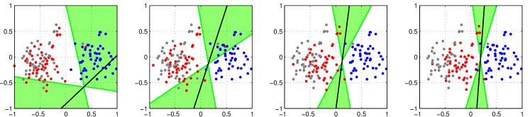
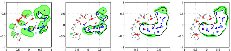
Figure 1: Two-dimensional examples of randomized prediction games, for SVMs with linear (top) and RBF kernels (bottom). Each row shows how the algorithm gradually converges to a Nash equilibrium. Blue (gray) points represent the legitimate (malicious) class. The mean of each manipulated attack sample is shown as a red point (for clarity, its variance is not shown). The black solid line represents the expected decision boundary, and the green shaded area highlights its variability within one standard deviation. Note how the linear SVM’s decision boundary tends to shift towards the legitimate class, while the nonlinear boundary provides a better enclosing of the same class. This intuitively allows for a higher robustness to different kinds of attack, as it requires the adversary to make a higher number of modifications to the attack samples to evade detection, at the expense of a higher number of misclassified legitimate samples.

IV Kernelization

Our game, as in Bruckner et al. [11], assumes explicit knowledge of the feature space $\phi$, where the data generator is assumed to randomize the samples $\dot{\boldsymbol{x}}=\phi(\boldsymbol{x})$. However, in many applications, the feature mapping is only implicitly given in terms of a positive semidefinite kernel function $k:\mathcal{X}\times\mathcal{X}\to\mathbb{R}$ that measures the similarity between samples as a scalar product in the corresponding kernel Hilbert space, i.e., there exists $\phi:\mathcal{X}\to\mathbb{R}$ such that $k(\boldsymbol{x},\boldsymbol{x}^{\prime})=\phi(\boldsymbol{x})^{\top}\phi(\boldsymbol{x}^{\prime})$. Note that in this setting the input space $\mathcal{X}$ is not restricted to a vector space like in the previous section (e.g. it might contain graphs or other structured entities).

For the representer theorem to hold [39], we assume that the randomized weight vectors of the learner live in the same subspace of the reproducing kernel Hilbert space, i.e., $\boldsymbol{w}=\sum_{j}\alpha_{j}\phi(\hat{\boldsymbol{x}}_{j})$, where $\boldsymbol{\alpha}\in\mathbb{R}^{\mathsf{n}}$. Analogously, we restrict the randomized samples obtained by the data generator to live in the span of the mapped training instances, i.e., $\dot{\boldsymbol{x}}_{i}=\sum_{j=1}^{\mathsf{n}}\xi_{ij}\phi(\hat{\boldsymbol{x}}_{j})$, where $\boldsymbol{\xi}_{i}=(\xi_{i1},\dots,\xi_{i\mathsf{n}})^{\top}\in\mathbb{R}^{\mathsf{n}}$.

Now, instead of randomizing $\boldsymbol{w}$ and $\dot{\mathtt{X}}$, we let the data generator and the learner randomize $\mathtt{\Xi}=(\boldsymbol{\xi}_{1},\dots,\boldsymbol{\xi}_{\mathsf{n}})$ and $\boldsymbol{\alpha}$, respectively. Moreover, we assume that the expected costs $\bar{c}_{l/d}$ can be rewritten in terms of $\boldsymbol{\alpha}$ and $\mathtt{\Xi}$ in a way that involves only inner products of $\phi(\boldsymbol{x})$, to take advantage of the kernel trick. This is clearly possible for the term $\boldsymbol{w}^{\top}\dot{\boldsymbol{x}}_{i}=\boldsymbol{\alpha}^{\top}\mathtt{K}\boldsymbol{\xi}_{i}$ in (1) and (2), where $\mathtt{K}$ is the kernel matrix. Hence, the applicability of the kernel trick only depends on the choice of the regularizers. It is easy to see that due to the linearity of the variable shift, existence and uniqueness of a Nash equilibrium in our kernelized game hold under the same conditions given for the linear case.

Although the data generator is virtually randomizing strategies in some subspace of the reproducing kernel Hilbert space, in reality manipulations should occur in the original input space. Hence, to construct the real attack samples $\{\boldsymbol{x}_{i}\}_{i=1}^{n}$ corresponding to the data generator’s strategy at the Nash equilibrium, one should solve the so-called pre-image problem, inverting the implicit feature mapping $\phi^{-1}(\mathtt{K}\boldsymbol{\xi}_{i})$ for each sample. This problem is in general neither convex, nor it admits a unique solution. However, reliable solutions can be easily found using well-principled approximations [39, 11]. It is finally worth remarking that solving the pre-image problem is not even required from the learner’s perspective, i.e., to train the corresponding, secure classification function.

V Discussion

In this section, we report a simple case study on a two-dimensional dataset to visually demonstrate the effect of randomized prediction games on SVM-based learners. From a pragmatic perspective, this example suggests also that uniqueness of the Nash Equilibrium should not be taken as a strict requirement in our game.

An instance of the proposed randomized prediction game for a linear SVM and for a non-linear SVM with the RBF kernel is reported in Fig. 1. As one may note from the plots, the main effect of simulating the presence of an attacker that manipulates malicious data to evade detection is to cause the linear decision boundary to gradually shift towards the legitimate class, and the nonlinear boundary to find a better enclosing of the legitimate samples. This should generally improve the learner’s robustness to any kind of evasion attempt, as it requires the attacker to mimic more carefully the feature values of legitimate samples – a task typically harder in several adversarial settings than just obfuscating the content of a malicious sample to make it sufficiently different from the known malicious ones [9, 7].

Based on this observation, any attempt aiming to satisfy the sufficient conditions for uniqueness of the Nash Equilibrium will result in an increase of the regularization strength in either the learner’s or the attacker’s cost function. Indeed, to satisfy the condition in Lem. 1, one could sufficiently increase $\rho_{l}$, $\rho_{d}$, or both. This amounts to increasing the regularization strength of either players, which in turn reduces in some sense their power. Hence, it should be clear that enforcing satisfaction of the sufficient conditions that guarantee the uniqueness of the Nash equilibrium might be counterproductive, by inducing the learner to weakly enclose the legitimate class, either due to a too strong regularization of the learners’ parameters, or by limiting the ability of the attacker to manipulate the malicious samples, thus allowing the leaner to keep a loose boundary. This will in general compromise the quality of the adversarial learning procedure. This argument shares similarities with the idea of addressing non-convex machine learning problems directly, without resorting to convex approximations [37, 38].

Besides improving classifier robustness, finding a better enclosure of the legitimate class may however cause a higher number of legitimate samples to be misclassified as malicious. There is indeed a trade-off between the desired level of robustness and the fraction of misclassified legitimate samples. The benefit of using randomization here is to make the attacker’s strategy less pessimistic than in the case of static prediction games [10, 11], which should allow us to eventually find a better trade-off between robustness and legitimate misclassifications. This aspect is investigated more systematically in the experiments reported in the next section.

VI Experiments

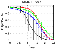
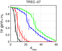
Figure 2: Security evaluation curves, reporting the average TP at FP=1% (along with its standard deviation, shown with error bars) against an increasing amount of manipulations to the attack samples (measured by $d_{\rm max}$), for handwritten digit (first and second plot), spam (third plot), and PDF (fourth plot) data.

In this section we present a set of experiments on handwritten digit recognition, spam filtering, and PDF malware detection. Despite handwritten digit recognition is not a proper adversarial learning task as spam and malware detection, we consider it in our experiments to provide a visual interpretation of how secure learning algorithms are capable of improving robustness to evasion attacks.

We consider only linear classifiers, as they are a typical choice in these settings, and especially in spam filtering [2, 14, 7]. This also allows us to carry out a fair comparison with state-of-the-art secure learning algorithms, as they yield linear classification functions. We compare our secure linear SVM learner (Sect. III) with the standard linear SVM implementation [40], and with the state-of-the-art robust classifiers InvarSVM [21, 22], and NashSVM [11] (see Sect. VII).

The goal of these experiments is to test whether these secure algorithms work well also under attack scenarios that differ from those hypothesized during design – a typical setting in security-related tasks; e.g., what happens if game-based classification techniques like that proposed in this paper and NashSVM are used against attackers that exploit a different attack strategy, i.e., attackers that may not act rationally according to the hypothesized objective function? What happens when the attacker does not play at the expected Nash equilibrium? These are rather important questions to address, as we do not have any guarantee that real-world attackers will play according to the hypothesized objective function.

Security evaluation. To address the above issues, we consider the security evaluation procedure proposed in [7]. It evaluates the performance of the considered classifiers under attack scenarios of increasing strength. We consider the True Positive (TP) rate (i.e., the fraction of detected attacks) evaluated at $1\%$ False Positive (FP) rate (i.e., the fraction of misclassified legitimate samples) as performance measure. We evaluate the performance of each classifier in the absence of attack, as in standard performance evaluation techniques, and then start manipulating the malicious test samples to simulate attacks of different strength. We assume a worst-case adversary, i.e., an adversary that has perfect knowledge of the attacked classifier, since we are interested in understanding the worst-case performance degradation. Note however that other choices are possible, depending on specific assumptions on the adversary’s knowledge and capability [14, 7, 13]. In this setting, we assume that the optimal (worst-case) sample manipulation $\mathbf{x}^{*}$ operated by the attacker is obtained by solving the following optimization problem:

$$\begin{array}[]{rl}\boldsymbol{x}^{*}\in\displaystyle\operatornamewithlimits{\arg\,\min}_{\boldsymbol{x}}&yf(\boldsymbol{x};\boldsymbol{w}),\\ {\rm s.t.}&d(\boldsymbol{x},\hat{\boldsymbol{x}_{i}})\leq d_{\rm max},\end{array}$$ (34)

where $y$ is the malicious class label, $d(\boldsymbol{x},\boldsymbol{x}_{i})$ measures the distance between the perturbed sample $\boldsymbol{x}$ and the $i^{\rm th}$ malicious data sample $\hat{\boldsymbol{x}_{i}}$ (in this case, we use the $\ell_{2}$ norm, as done by the considered classifiers). The maximum amount of modifications is bounded by $d_{\rm max}$, which is a parameter representing the attack strength. It is obvious that the more modifications the adversary is allowed to make on the attack samples, the higher the performance degradation incurred by the classifier is expected to be. Accordingly, the performance of more secure classifiers is expected to degrade more gracefully as the attack strength increases [14, 7].

The solution of the above problem is trivial when we consider linear classifiers, the Euclidean distance, and $\mathbf{x}$ is unconstrained: it amounts to setting $\boldsymbol{x}^{*}=\hat{\boldsymbol{x}_{i}}-yd_{\rm max}\frac{\mathbf{w}}{||\mathbf{w}||}$. If $\mathbf{x}$ lies within some constrained domain, e.g. $[0,1]$, then one may consider a simple gradient descent with box constraints on $\mathbf{x}$ (see, e.g., [9]). If $\mathbf{x}$ takes on binary values, e.g., $\{0,1\}$, then the attack amounts to switching from $0$ to $1$ or vice-versa the value of a maximum of $d_{\max}$ features which have been assigned the highest absolute weight values by the classifier. In particular, if $y\,w_{k}>0$ ($y\,w_{k}<0$) and the $k$-th feature satisfies $\hat{x}_{ik}=1$ ($\hat{x}_{ik}=0$), then $x^{*}_{k}=1$ ($x^{*}_{k}=0$) [14, 7].

Parameter selection. The considered methods require setting different parameters. From the learners’ perspective, we have to tune the regularization parameter $C$ for the standard linear SVM and InvarSVM, while we respectively have $\rho_{-1}$ and $\rho_{l}$ for NashSVM and for our method. In addition, the robust classifiers require setting the parameters of their attacker’s objective. For InvarSVM, we have to set $K$, i.e., the number of modifiable features, while for NashSVM and for our method, we have to set the value of the regularization parameter $\rho_{+1}$ and $\rho_{d}$, respectively. Further, to guarantee existence of a Nash Equilibrium point, we have to enforce some box constraints on the distribution’s parameters. For the attacker, we restrict the mean of the attack points to lie in $[0,1]$ (as the considered datasets are normalized in that interval), and their variance in $[10^{-3},0.5]$. For the learner, the variance of $\boldsymbol{w}$ is allowed to vary in $[10^{-6},10^{-3}]$, while its mean takes values on $[-W,W]$, where $W$ is optimized together with the other parameters. All the above mentioned parameters are set by performing a grid-search on the parameter space $(C$, $\rho_{-1}$, $\rho_{d}\in\{0.01,0.1,1,10,100\}$; $K\in\{8,13,25,30,47,52,63\}$; $\rho_{+1},\rho_{d}\in\{0.01,0.05,0.1,1,10\}$; $W\in\{0.01,0.05,0.1,1\})$, and retaining the parameter values that maximize the area under the security evaluation curve on a validation set. The reason is to find a parameter configuration for each method that attains the best average robustness over all attack intensities (values of $d_{\rm max}$), i.e. the best average TP rate at FP=$1\%$.

VI-A Handwritten Digit Recognition

Similarly to [21], we focus on two two-class sub-problems of discriminating between two distinct digits from the MNIST dataset [41], i.e. 1 vs 3, and 6 vs 7, where the second digit in each pair represents the attacking class ($y=+1$). The digits are originally represented as gray-scale images of $28\times 28$ pixels. They are simply mapped to feature vectors by ordering the pixels in raster scan order. The overall number of features is thus $d=784$. We normalize each feature (pixel value) in $[0,1]$, by dividing its value by $255$. We build a training and a validation set of 1,000 samples each by randomly sampling the original training data available for MNIST. As for the test set, we use the default set provided with this data, which consists of approximately 1,000 samples for each digit (class). The results averaged on $5$ repetitions are shown in the first and second plot of Fig. 2 respectively for 1 vs 3, and 6 vs 7. As one may notice, in the absence of attack (i.e. when $d_{\rm max}=0$), all classifiers achieved comparable performance (the TP rate is almost 100% for all of them), due to a conservative choice of the operating point (FP=$1\%$), that should also guarantee a higher robustness against the attack. In the presence of attack, our approach (RNashSVM) exhibits comparable performance to NashSVM on the problem of discriminating 1 vs 3, and to InvarSVM on 6 vs 7. NashSVM outperforms the standard SVM implementation in both cases, but exhibits lower security (robustness) than InvarSVM on 6 vs 7, despite the attacker’s regularizer in InvarSVM is not even based on the $\ell_{2}$ norm.

Figure 3: Examples of obfuscated digits against each classifier when $d_{\rm max}=2.5$ for 1 vs 3 (top row), and when $d_{\rm max}=5$ for 6 vs 7 (bottom row).

Finally, in Fig. 3 we report two attack samples (a digit from class 1 and one from class 6) and show how they are obfuscated by the attack strategy of Eq. (34) to evade detection against each classifier. Notice how the original attacking samples (1 and 6) tend to resemble more the corresponding attacked classes (3 and 7) when natively robust classifiers are used. This visual example confirms the analysis of Sect. V, i.e., that higher robustness is achieved when the adversary is required to mimic the feature values of samples of the legitimate class, instead of slightly modifying the attack samples to differentiate them from the rest of the malicious data.

VI-B Spam Filtering

In these experiments we use the benchmark, publicly available, TREC 2007 email corpus [42], which consists of 75,419 real emails (25,220 legitimate and 50,199 spam messages) collected between April and July 2007. We exploit the bag-of-words feature model, in which each binary feature denotes the absence ($0$) or presence ($1$) of the corresponding word in a given email [13, 14, 7, 11]. Features (words) are extracted from training emails using the tokenization method of the widely-known anti-spam filter SpamAssassin, and then $n=1,000$ distinct features are selected using a supervised feature selection approach based on the information gain criterion [43]. We build a training and a validation set of 1,000 samples each by randomly sampling the first 5,000 emails in chronological order of the original dataset, while a test set of about 2,000 samples is randomly sampled from the subsequent set of 5,000 emails. The results averaged on $5$ repetitions are shown in the third plot of Fig. 2. As in the previous case, in the absence of attack ($d_{\rm max}=0$) all the classifiers exhibit a very high (and similar) performance. However, as the attack intensity ($d_{\rm max}$) increases, their performance degrades more or less gracefully, i.e. their robustness to the attack is different. Surprisingly, one may notice that only InvarSVM and RNashSVM exhibited an improved level of security. The reason is that these two classifiers are able to find a more uniform set of weights than SVM and NashSVM, and, in this case, this essentially requires the adversary to manipulate a higher number of features to significantly decrease the value of the classifier’s discriminant function. Note that a similar result has been heuristically found also in [13, 14].

VI-C PDF Malware Detection

We consider here another relevant application example in computer security, i.e., the detection of malware in PDF files. The main reason behind the diffusion of malware in PDF files is that they exhibit a very flexible structure that allows embedding several kinds of resources, including Flash, JavaScript and even executable code. Resources simply consists of keywords that denote their type, and of data streams that contain the actual object; e.g., an embedded resource in a PDF file may be encoded as follows:

13 0 obj << /Kids [ 1 0 R 11 0 R ]
/Type /Page ... >> end obj

where keywords are highlighted in bold face. Recent work has exploited machine learning techniques to discriminate between malicious and legitimate PDF files, based on the analysis of their structure and, in particular, of the embedded keywords [44, 45, 46, 47, 48]. We exploit here a similar feature representation to that proposed in [45], where each feature denotes the presence of a given keyword in the PDF file. We collected 5993 recent malware samples from the Contagio dataset, and 5951 benign samples from the web. Following the procedure described in [45], we extracted 114 keywords from the first 1,000 samples (in chronological order) to build our feature set. Then, we build training, validation and test sets as in the spam filtering case, and average results over $5$ repetitions. Attacks in this case are simulated by allowing the attacker only to increase the feature values of malicious samples, which corresponds to adding the constraint $\boldsymbol{x}\geq\hat{\boldsymbol{x}}_{i}$ (where the inequality holds for all features) to Problem 34. The reason is that removing objects (and keywords) from malicious PDFs may compromise the intrusive nature of the embedded exploitation code, whereas adding objects can be easily done through the PDF versioning mechanism [46, 9, 48].

Results are shown in the $4$th plot of Fig. 2. The considered methods mostly exhibit the same behavior shown in the spam filtering case, besides the fact that, here, there is a clearer trade-off between the performance in the absence of attack, and robustness under attack. In particular, InvarSVM and RNashSVM are significantly more robust under attack (i.e., when $d_{\rm max}>0$) than SVM and NashSVM, at the expense of a slightly worsened detection rate in the absence of attack (i.e., when $d_{\rm max}=0$).

To summarize, the reported experiments show that, even if the attacker does not play the expected attack strategy at the Nash equilibrium, most of the proposed state-of-the-art secure classifiers are still able to outperform classical techniques, and, in particular, that the proposed RNashSVM classifier may guarantee an even higher level of robustness. Understanding how this property relates to the use of probability distributions over the set of the classifier’s and of the attacker’s strategies remains an interesting future question.

VII Related Work

The problem of devising secure classifiers against different kinds of manipulation of samples at test time has been widely investigated in previous work [1, 21, 22, 23, 6, 10, 24, 11, 25, 26, 27]. Inspired by the seminal work by Dalvi et al. [1], several authors have proposed a variety of modifications to existing learning algorithms to improve their security against different kinds of attack. Globerson et al. [21, 22] have formulated the so-called Invariant SVM (InvarSVM) in terms of a minimax approach (i.e., a zero-sum game) to deal with worst-case feature manipulations at test time, including feature addition, deletion, and rescaling. This work has been further extended in [23] to allow features to have different a-priori importance levels, instead of being manipulated equally likely. Notably, more recent research has also considered the development of secure learning algorithms based on zero-sum games for sensor networks, including distributed secure algorithms [27] and algorithms for detecting adversarially-corrupted sensors [26].

The rationale behind shifting from zero-sum to non-zero-sum games for adversarial learning is that the classifier and the attacker may not necessarily aim at maximizing antagonistic objective functions. This in turn implies that modeling the problem as a zero-sum game may lead one to design overly-pessimistic classifiers, as pointed out in [11]. Even considering a non-zero-sum Stackelberg game may be too pessimistic, since the attacker (follower) is supposed to move after the classifier (leader), while having full knowledge of the chosen classification function (which again is not realistic in practical settings) [24, 11]. For these reasons, Brückner et al. [10, 11] have formalized adversarial learning as a non-zero-sum game, referred to as static prediction game. Assuming that the players act simultaneously (conversely to Stackelberg games [24]), they devised conditions under which a unique Nash equilibrium for this game exists, and developed algorithms for learning the corresponding robust classifiers, including the so-called NashSVM. Our work essentially extends this approach by introducing randomization over the players’ strategies.

For completeness, we also mention here that in [25] Bayesian games for adversarial regression tasks have been recently proposed. In such games, uncertainty on the objective function’s parameters of either player is modeled by considering a probability distribution over their possible values. To the best of our knowledge, this is the first attempt towards modeling the uncertainty of the attacker and the classifier on the opponent’s objective function.

VIII Conclusions and Future Work

In this paper, we have extended the work in [11] by introducing randomized prediction games. To operate this shift, we have considered parametrized, bounded families of probability distributions defined over the set of pure strategies of either players. The underlying idea, borrowed from [28, 3, 6], consists of randomizing the classification function to make the attacker select a less effective attack strategy. Our experiments, conducted on an handwritten digit recognition task and on realistic application examples involving spam and malware detection, show that competitive, secure SVM classifiers can be learnt using our approach, even when the conditions behind uniqueness of the Nash equilibrium may not hold, i.e., when the attacker may not play according to the objective function hypothesized for her by the classifier. This mainly depends on the particular kind of decision function learnt by the learning algorithm under our game setting, which tends to find a better ‘enclosing’ of the legitimate class. This generally requires the attacker to make more modifications to the malicious samples to evade detection, regardless of the attack strategy chosen. We can thus argue that the proposed methods exhibit robustness properties particularly suited to adversarial learning tasks. Moreover, the fact that the proposed methods may perform well also when the Nash equilibrium is not guaranteed to be unique suggests us that the conditions behind its uniqueness may hold under less restrictive assumptions (e.g., when the SVM admits a unique solution [35, 36]). We thus leave a deeper investigation of this aspect to future work.

Another interesting extension of this work may be to apply randomized prediction games in the context of unsupervised learning, and, in particular, clustering algorithms. It has been recently shown that injecting a small percentage of well-crafted poisoning attack samples into the input data may significantly subvert the clustering process, compromising the subsequent data analysis [49, 50]. In this respect, we believe that randomized prediction games may help devising secure countermeasures to mitigate the impact of such attacks; e.g., by explicitly modeling the presence of poisoning samples (generated according to a probability distribution chosen by the attacker) during the clustering process.

It is worth finally mentioning that our work is also slightly related to previous work on security games, in which the goal of the defender is to adopt randomized strategies to protect his or her assets from the attacker, by allocating a limited number of defensive resources; e.g., police officers for airport security, protection mechanisms for network security [51, 52, 53]. Although our game is not directly concerned to the protection of a given set of assets, we believe that investigating how to bridge the proposed approach within this well-grounded field of study may provide promising research directions for future work, e.g., in the context of network security [52, 53], or for suggesting better user attitudes towards security issues [54]. This may also suggest interesting theoretical advancements; e.g., to establish conditions for the equivalence of Nash and Stackelberg games [51], and to address issues related to the uncertainty on the players’ strategies, or on their (sometimes bounded) rationality, e.g., through the use of Bayesian games [25], security strategies and robust optimization [52, 53]. Another suggestion to overcome the aforementioned issues is to exploit higher-level models of the interactions between attackers and defenders in complex, real-world problems; e.g., through the use of replicator equations to model adversarial dynamics in security-related tasks [55]. Exploiting conformal prediction may be also an interesting research direction towards improving current adversarial learning systems [56]. To conclude, we believe these are all relevant research directions for future work.

Samuel Rota Bulò received his PhD in computer science at the University of Venice, Italy, in 2009 and he worked as a postdoctoral researcher at the same institution until 2013. He is currently a researcher of the “Technologies of Vision” laboratory at Fondazione Bruno Kessler in Trento, Italy. His main research interests are in the areas of computer vision and pattern recognition with particular emphasis on discrete and continuous optimisation methods, graph theory and game theory. Additional research interests are in the field of stochastic modelling. He regularly publishes his research in well-recognized conferences and top-level journals mainly in the areas of computer vision and pattern recognition. He held research visiting positions at the following institutions: IST - Technical University of Lisbon, University of Vienna, Graz University of Technology, University of York (UK), Microsoft Research Cambridge (UK) and University of Florence.

Battista Biggio (M’07) received the M.Sc. degree (Hons.) in Electronic Engineering and the Ph.D. degree in Electronic Engineering and Computer Science from the University of Cagliari, Italy, in 2006 and 2010. Since 2007, he has been with the Department of Electrical and Electronic Engineering, University of Cagliari, where he is currently a post-doctoral researcher. In 2011, he visited the University of Tübingen, Germany, and worked on the security of machine learning to training data poisoning. His research interests include secure machine learning, multiple classifier systems, kernel methods, biometrics and computer security. Dr. Biggio serves as a reviewer for several international conferences and journals. He is a member of the IEEE and of the IAPR.

Ignazio Pillai received the M.Sc. degree in Electronic Engineering, with honors, and the Ph.D. degree in Electronic Engineering and Computer Science from the University of Cagliari, Italy, in 2002 and 2007, respectively. Since 2003 he has been working for the Department of Electrical and Electronic Engineering at the University of Cagliari, Italy, where he is a post doc in the research laboratory on pattern recognition and applications. His main research topics are related to multi-label classification, multimedia document categorization and classification with a reject option. He has published about twenty papers in international journals and conferences, and acts as a reviewer for several international conferences and journals.

Marcello Pelillo joined the faculty of the University of Bari, Italy, as an Assistant professor of computer science in 1991. Since 1995, he has been with the University of Venice, Italy, where he is currently a Full Professor of Computer Science. He leads the Computer Vision and Pattern Recognition Group and has served from 2004 to 2010 as the Chair of the board of studies of the Computer Science School. He held visiting research positions at Yale University, the University College London, McGill University, the University of Vienna, York University (UK), and the National ICT Australia (NICTA). He has published more than 130 technical papers in refereed journals, handbooks, and conference proceedings in the areas of computer vision, pattern recognition and neural computation. He serves (or has served) on the editorial board for the journals IEEE Transactions on Pattern Analysis and Machine Intelligence, Pattern Recognition and IET Computer Vision, and is regularly on the program committees of the major international conferences and workshops of his fields. In 1997, he co-established a new series of international conferences devoted to energy minimization methods in computer vision and pattern recognition (EMMCVPR). He is (or has been) scientific coordinator of several research projects, including SIMBAD, an EU-FP7 project devoted to similarity-based pattern analysis and recognition. Prof. Pelillo is a Fellow of the IAPR and Fellow of the IEEE.

Fabio Roli (F’12) received his Ph.D. in Electronic Engineering from the University of Genoa, Italy. He was a research group member of the University of Genoa (88-94). He was adjunct professor at the University of Trento (’93-’94). In 1995, he joined the Department of Electrical and Electronic Engineering of the University of Cagliari, where he is now professor of Computer Engineering and head of the research laboratory on pattern recognition and applications. His research activity is focused on the design of pattern recognition systems and their applications. He was a very active organizer of international conferences and workshops, and established the popular workshop series on multiple classifier systems. Dr. Roli is Fellow of the IEEE and of the IAPR.

References

- [1] N. Dalvi, P. Domingos, Mausam, S. Sanghai, and D. Verma, “Adversarial classification,” in Tenth ACM SIGKDD Int’l Conf. on Knowledge Discovery and Data Mining (KDD), Seattle, 2004, pp. 99–108.
- [2] D. Lowd and C. Meek, “Adversarial learning,” in Proc. 11th ACM SIGKDD International Conference on Knowledge Discovery and Data Mining (KDD). Chicago, IL, USA: ACM Press, 2005, pp. 641–647.
- [3] M. Barreno, B. Nelson, R. Sears, A. D. Joseph, and J. D. Tygar, “Can machine learning be secure?” in Symp. Inform., Comp. and Comm. Sec., ser. ASIACCS ’06. New York, NY, USA: ACM, 2006, pp. 16–25.
- [4] A. A. Cárdenas and J. S. Baras, “Evaluation of classifiers: Practical considerations for security applications,” in AAAI Workshop on Evaluation Methods for Machine Learning, Boston, MA, USA, July, 16-20 2006.
- [5] P. Laskov and M. Kloft, “A framework for quantitative security analysis of machine learning,” in AISec ’09: 2nd ACM Workshop on Sec. and Artificial Intell.. New York, NY, USA: ACM, 2009, pp. 1–4.
- [6] L. Huang, A. D. Joseph, B. Nelson, B. Rubinstein, and J. D. Tygar, “Adversarial machine learning,” in 4th ACM Workshop on Artificial Intell. and Sec. (AISec), Chicago, IL, USA, 2011, pp. 43–57.
- [7] B. Biggio, G. Fumera, and F. Roli, “Security evaluation of pattern classifiers under attack,” IEEE Transactions on Knowledge and Data Engineering, vol. 26, no. 4, pp. 984–996, April 2014.
- [8] B. Biggio, I. Corona, B. Nelson, B. Rubinstein, D. Maiorca, G. Fumera, G. Giacinto, and F. Roli, “Security evaluation of support vector machines in adversarial environments,” in Support Vector Machines Applications, Y. Ma and G. Guo, Eds. Springer Int’l Publishing, 2014, pp. 105–153.
- [9] B. Biggio, I. Corona, D. Maiorca, B. Nelson, N. Šrndić, P. Laskov, G. Giacinto, and F. Roli, “Evasion attacks against machine learning at test time,” in European Conf. Mach. Learn. and Principles and Practice of Knowl. Disc. in Databases (ECML PKDD), Part III, ser. LNCS, H. Blockeel, K. Kersting, S. Nijssen, and F. Železný, Eds., vol. 8190. Springer Berlin Heidelberg, 2013, pp. 387–402.
- [10] M. Brückner and T. Scheffer, “Nash equilibria of static prediction games,” in NIPS 22, Y. Bengio et al., Eds. MIT Press, 2009, pp. 171–179.
- [11] M. Brückner, C. Kanzow, and T. Scheffer, “Static prediction games for adversarial learning problems,” J. Mach. Learn. Res., vol. 13, pp. 2617–2654, September 2012.
- [12] G. L. Wittel and S. F. Wu, “On attacking statistical spam filters,” in 1st Conf. Email and Anti-Spam (CEAS), Mountain View, CA, USA, 2004.
- [13] A. Kolcz and C. H. Teo, “Feature weighting for improved classifier robustness,” in 6th Conf. Email and Anti-Spam (CEAS), Mountain View, CA, USA, 2009.
- [14] B. Biggio, G. Fumera, and F. Roli, “Multiple classifier systems for robust classifier design in adversarial environments,” Int’l J. Mach. Learn. and Cybernetics, vol. 1, no. 1, pp. 27–41, 2010.
- [15] M. Christodorescu, S. Jha, S. Seshia, D. Song, and R. Bryant, “Semantics-aware malware detection,” in IEEE Symp. Security and Privacy, May 2005, pp. 32–46.
- [16] P. Fogla, M. Sharif, R. Perdisci, O. Kolesnikov, and W. Lee, “Polymorphic blending attacks,” in USENIX-SS’06: 15th Conf. USENIX Sec. Symp.. Berkeley, CA, USA: USENIX Association, 2006, pp. 241–256.
- [17] B. Nelson, M. Barreno, F. J. Chi, A. D. Joseph, B. I. P. Rubinstein, U. Saini, C. Sutton, J. D. Tygar, and K. Xia, “Exploiting machine learning to subvert your spam filter,” in LEET’08: 1st USENIX Workshop on Large-Scale Exploits and Emergent Threats. Berkeley, CA, USA: USENIX Association, 2008, pp. 1–9.
- [18] B. I. Rubinstein, B. Nelson, L. Huang, A. D. Joseph, S.-h. Lau, S. Rao, N. Taft, and J. D. Tygar, “Antidote: understanding and defending against poisoning of anomaly detectors,” in 9th ACM Internet Measurement Conf., ser. IMC ’09. New York, NY, USA: ACM, 2009, pp. 1–14.
- [19] B. Biggio, B. Nelson, and P. Laskov, “Poisoning attacks against support vector machines,” in 29th Int’l Conf. Mach. Learn., J. Langford and J. Pineau, Eds. Omnipress, 2012, pp. 1807–1814.
- [20] H. Xiao, B. Biggio, G. Brown, G. Fumera, C. Eckert, and F. Roli, “Is feature selection secure against training data poisoning?” in JMLR W&CP - 32nd Int’l Conf. Mach. Learn., F. Bach and D. Blei, Eds., vol. 37, 2015, pp. 1689–1698.
- [21] A. Globerson and S. T. Roweis, “Nightmare at test time: robust learning by feature deletion,” in 23rd Int’l Conf. Mach. Learn., W. W. Cohen and A. Moore, Eds., vol. 148. ACM, 2006, pp. 353–360.
- [22] C. H. Teo, A. Globerson, S. Roweis, and A. Smola, “Convex learning with invariances,” in NIPS 20, J. Platt, D. Koller, Y. Singer, and S. Roweis, Eds. Cambridge, MA: MIT Press, 2008, pp. 1489–1496.
- [23] O. Dekel, O. Shamir, and L. Xiao, “Learning to classify with missing and corrupted features,” Machine Learning, vol. 81, pp. 149–178, 2010.
- [24] M. Brückner and T. Scheffer, “Stackelberg games for adversarial prediction problems,” in 17th ACM Int’l Conf. Knowl. Disc. and Data Mining, ser. KDD ’11. New York, NY, USA: ACM, 2011, pp. 547–555.
- [25] M. Großhans, C. Sawade, M. Brückner, and T. Scheffer, “Bayesian games for adversarial regression problems,” in JMLR W&CP - 30th Int’l Conf. Mach. Learn., vol. 28, no. 3, 2013, pp. 55–63.
- [26] K. Vamvoudakis, J. Hespanha, B. Sinopoli, and Y. Mo, “Detection in adversarial environments,” IEEE Transactions on Automatic Control, vol. 59, no. 12, pp. 3209–3223, Dec 2014.
- [27] R. Zhang and Q. Zhu, “Secure and resilient distributed machine learning under adversarial environments,” in 18th Int’l Conf. on Information Fusion. IEEE, July 2015, pp. 644–651.
- [28] B. Biggio, G. Fumera, and F. Roli, “Adversarial pattern classification using multiple classifiers and randomisation,” in 12th Joint IAPR Int’l Workshop on Structural and Syntactic Patt. Rec., ser. LNCS, vol. 5342. Orlando, Florida, USA: Springer-Verlag, 2008, pp. 500–509.
- [29] I. L. Glicksberg, “A further generalization of the Kakutani fixed point theorem, with application to Nash equilibrium,” Proceedings of the American Mathematical Society, vol. 3, no. 1, pp. 170–174, 1952.
- [30] J. B. Rosen, “Existence and uniqueness of equilibrium points for concave n-person games,” Econometrica, vol. 33, no. 3, pp. 520–534, 1965.
- [31] D. Zhu and P. Marcotte, “Modified descent methods for solving the monotone variational inequality problem,” Operations Research Letters, vol. 14, no. 2, pp. 111–120, 1993.
- [32] P. T. Harker and J. Pang, “Finite-dimensional variational inequality and nonlinear complementary problems: A survey of theory, algorithms and applications,” Math. Programming, vol. 48, no. 2, pp. 161–220, 1990.
- [33] C. Geiger and C. Kanzow, Theorie und Numerik restringierter Optimimierungsaufgaben. Springer, 1999.
- [34] C. Cortes and V. N. Vapnik, “Support-vector networks,” Machine Learning, vol. 20, 1995.
- [35] S. Abe, “Analysis of support vector machines,” in Proc. 12th IEEE Workshop on Neural Networks for Signal Processing, 2002, pp. 89–98.
- [36] C. J. C. Burges and D. J. Crisp, “Uniqueness of the SVM solution,” in NIPS, S. A. Solla, T. K. Leen, and K.-R. Müller, Eds. The MIT Press, 1999, pp. 223–229.
- [37] R. Collobert, F. Sinz, J. Weston, and L. Bottou, “Trading convexity for scalability,” in 23rd Int’l Conf. Mach. Learn., ser. ICML ’06. New York, NY, USA: ACM, 2006, pp. 201–208.
- [38] Y. Bengio and Y. LeCun, “Scaling learning algorithms towards AI,” in Large Scale Kernel Machines, L. Bottou, O. Chapelle, D. DeCoste, and J. Weston, Eds. MIT Press, 2007.
- [39] B. Schölkopf, S. Mika, C. J. C. Burges, P. Knirsch, K.-R. Muller, G. Rätsch, and A. J. Smola, “Input space versus feature space in kernel-based methods.” IEEE Trans. Neural Networks, vol. 10, no. 5, pp. 1000–1017, 1999.
- [40] C.-C. Chang and C.-J. Lin, “LibSVM: a library for support vector machines,” 2001.
- [41] Y. LeCun, L. Jackel, L. Bottou, A. Brunot, C. Cortes, J. Denker, H. Drucker, I. Guyon, U. Müller, E. Säckinger, P. Simard, and V. Vapnik, “Comparison of learning algorithms for handwritten digit recognition,” in Int’l Conf. on Artificial Neural Networks, 1995, pp. 53–60.
- [42] G. V. Cormack, “Trec 2007 spam track overview,” in TREC, E. M. Voorhees and L. P. Buckland, Eds., vol. Special Publication 500-274. National Institute of Standards and Technology (NIST), 2007.
- [43] G. Brown, A. Pocock, M.-J. Zhao, and M. Luján, “Conditional likelihood maximisation: A unifying framework for information theoretic feature selection,” J. Mach. Learn. Res., vol. 13, pp. 27–66, 2012.
- [44] C. Smutz and A. Stavrou, “Malicious PDF detection using metadata and structural features,” in 28th Annual Computer Security App. Conf., ser. ACSAC ’12. New York, NY, USA: ACM, 2012, pp. 239–248.
- [45] D. Maiorca, G. Giacinto, and I. Corona, “A pattern recognition system for malicious pdf files detection,” in Machine Learning and Data Mining in Patt. Rec., ser. LNCS, P. Perner, Ed., vol. 7376. Springer Berlin Heidelberg, 2012, pp. 510–524.
- [46] D. Maiorca, I. Corona, and G. Giacinto, “Looking at the bag is not enough to find the bomb: an evasion of structural methods for malicious pdf files detection,” in 8th ACM Symp. Inform., Comp. and Comm. Sec., ser. ASIACCS ’13. New York, NY, USA: ACM, 2013, pp. 119–130.
- [47] N. Šrndić and P. Laskov, “Detection of malicious pdf files based on hierarchical document structure,” in 20th Annual Network & Distributed System Security Symposium (NDSS). The Internet Society, 2013.
- [48] N. Šrndic and P. Laskov, “Practical evasion of a learning-based classifier: A case study,” in Proc. 2014 IEEE Symp. Security and Privacy, ser. SP ’14. Washington, DC, USA: IEEE CS, 2014, pp. 197–211.
- [49] B. Biggio, I. Pillai, S. R. Bulò, D. Ariu, M. Pelillo, and F. Roli, “Is data clustering in adversarial settings secure?” in W. on Artificial Intell. and Sec., ser. AISec ’13. New York, NY, USA: ACM, 2013, pp. 87–98.
- [50] B. Biggio, S. R. Bulò, I. Pillai, M. Mura, E. Z. Mequanint, M. Pelillo, and F. Roli, “Poisoning complete-linkage hierarchical clustering,” in Joint IAPR Int’l W. on Structural, Syntactic, and Statistical Patt. Rec., ser. LNCS, P. Franti et al., Eds., vol. 8621. Joensuu, Finland: Springer Berlin Heidelberg, 2014, pp. 42–52.
- [51] D. Korzhyk, Z. Yin, C. Kiekintveld, V. Conitzer, and M. Tambe, “Stackelberg vs. nash in security games: an extended investigation of interchangeability, equivalence, and uniqueness,” J. Artif. Int. Res., vol. 41, no. 2, pp. 297–327, 2011.
- [52] T. Alpcan and T. Başar, Network security: A decision and game-theoretic approach. Cambridge University Press, 2010.
- [53] M. Tambe, Security and game theory: Algorithms, deployed systems, lessons learned. Cambridge University Press, 2011.
- [54] J. Grossklags, N. Christin, and J. Chuang, “Secure or insure?: A game-theoretic analysis of information security games,” in 17th Int’l Conf. on World Wide Web, ser. WWW ’08. New York, NY, USA: ACM, 2008, pp. 209–218.
- [55] G. Cybenko and C. E. Landwehr, “Security analytics and measurements,” IEEE Security & Privacy, vol. 10, no. 3, pp. 5–8, 2012.
- [56] H. Wechsler, “Cyberspace security using adversarial learning and conformal prediction,” Intelligent Information Management, vol. 7, no. 4, pp. 195–222, July 2015.