Stochastic Bouncy Particle Sampler

Abstract

We introduce a stochastic version of the non-reversible, rejection-free Bouncy Particle Sampler (BPS), a Markov process whose sample trajectories are piecewise linear, to efficiently sample Bayesian posteriors in big datasets. We prove that in the BPS no bias is introduced by noisy evaluations of the log-likelihood gradient. On the other hand, we argue that efficiency considerations favor a small, controllable bias, in exchange for faster mixing. We introduce a simple method that controls this trade-off. We illustrate these ideas in several examples which outperform previous approaches.

1 Introduction

The advent of the Big Data era presents special challenges to practitioners of Bayesian modeling because typical sampling-based inference methods have a computational cost per sample linear in the size of the dataset. This computational burden has been addressed in recent years through two major approaches (see (Bardenet et al., 2015) for a recent overview): (i) split the data into batches and combine posterior samples obtained in parallel from each batch, or (ii) use variants of the Markov Chain Monte Carlo (MCMC) algorithm that only query a subset of the data at every iteration. Our interest in the paper is in the latter approach, where many methods are based on modifying both steps of the Metropolis-Hastings (MH) algorithm: in the proposal step, only a mini-batch of the data is used, and the accept-reject step is either ignored or approximated (Korattikara et al., 2013; Bardenet et al., 2014). This strategy has been explored using proposals from Langevin (Welling & Teh, 2011), Riemannian Langevin (Patterson & Teh, 2013), Hamiltonian (Chen et al., 2014) and Riemannian Hamiltonian (Ma et al., 2015) dynamics. Other relevant works include (Ahn et al., 2012; Ding et al., 2014).

Despite the success of the above approach, the partial accept-reject step is a source of bias, the precise size of which is difficult to control, and which tends to be amplified by the noisy evaluation of the gradient. This has motivated the search for unbiased stochastic samplers, such as the Firefly MCMC algorithm (Maclaurin & Adams, 2014), the debiased pseudolikelihood approach of (Quiroz et al., 2016), and the quasi-stationary distribution approach of (Pollock et al., 2016).

The present work is motivated by the idea that the bias could be reduced by starting from a rejection-free MCMC algorithm, avoiding thus the Metropolis-Hastings algorithm altogether. Two similar algorithms of this type have been recently proposed: the Bouncy Particle Sampler (BPS) (Peters & de With, 2012; Bouchard-Côté et al., 2015), and Zig-Zag Monte Carlo (Bierkens & Roberts, 2015; Bierkens et al., 2016). These algorithms sample from the target distribution through non-reversible, piecewise linear Markov processes. Non-reversibility (i.e., the failure to satisfy detailed balance) has been shown in many cases to yield faster mixing rates (Neal, 2004; Vucelja, 2014; Bouchard-Côté et al., 2015).

Our contributions in this paper are twofold. Firstly, we show that the BPS algorithm is particularly well suited to sample from posterior distributions of big datasets, because the target distribution is invariant under zero-mean noisy perturbations of the log-likelihood gradient, such as those introduced by using mini-batches of the full dataset in each iteration.

Stochastic variants of BPS or Zig-Zag that preserve exactly the target distribution have been proposed, such as Local BPS (Bouchard-Côté et al., 2015) or Zig-Zag with subsampling (ZZ-SS) (Bierkens et al., 2016), but they lead to extremely slow mixing because are based on overly conservative bounds (which moreover must be derived on a case-by-case basis, and in many cases may not hold at all). This leads us to our second contribution, the Stochastic Bouncy Particle Sampler (SBPS), a stochastic version of the BPS algorithm which trades a small amount of bias for significantly reduced variance, yielding superior performance (and requiring no parameter tuning or derivation of problem-specific bounds) compared to existing subsampling-based Monte Carlo methods. SBPS inherits the piecewise linear sample paths of BPS, and therefore enjoys faster convergence of empirical means, particularly of rapidly varying test functions, compared to more standard approaches.

We organize this paper as follows. In Section 2 we review the Bouncy Particle Sampler, in Section 3 we study the invariance of the target distribution under noise perturbations to the BPS updates, in Section 4 we introduce SBPS, and in Section 5 a preconditioned variant. In Section 6 we discuss related works and in Section 7 we illustrate the advantages of SBPS in several examples.

2 The Bouncy Particle Sampler

Figure 1: Noisy vs. noiseless gradients in BPS. Above: Contour plot of the 2D density considered and sample BPS trajectories during 50 bounces, with exact and noisy gradients. The noise was sampled in each component from a ${\cal N}(0,5^{2})$ distribution. Below, Left: smoothed histogram of travel times until bouncing, with shorter times for noisy gradients. Middle: QQ-plot of one of the coordinates, showing that the invariant distribution is not changed by the noise. Right: ACFs of one of the coordinates, with slower mixing per iteration in the noisy case. However, note that these ACF plots do not account for computational cost per iteration.

Consider a distribution $p({\bf w})\propto e^{-U({\bf w})}\,,{\bf w}\in\mathbb{R}^{D}$, where the normalization factor may be intractable. The Bouncy Particle Sampler (BPS), proposed in (Peters & de With, 2012; Monmarché, 2014) and formalized and developed in (Bouchard-Côté et al., 2015), introduces a random velocity vector ${\bf v}$ distributed uniformly in the unit sphere $S^{D-1}$, and defines a continuous Markov process in $({\bf w},{\bf v})$. To describe this process we begin in discrete time and then take the continuous-time limit. Denoting time by $t$, consider a discrete-time Markov process that acts on the variables $({\bf w},{\bf v})$ as

$$({\bf w},{\bf v})_{t+\Delta t}=\left\{\!\!\!\!\!\begin{array}[]{rl}({\bf w}\!+\!{\bf v}\Delta t,{\bf v})&\!\!\!\!\!\textrm{w/prob. }1-\Delta t[G]_{+}\\ ({\bf w}\!+\!{\bf v}\Delta t,{\bf v}_{r})&\!\!\!\!\textrm{w/prob. }\Delta t[G]_{+}\end{array}\right.$$ (3)

where

$$[x]_{+}=\max(x,0)\,,$$ (4)

$$G={\bf v}\cdot\nabla U({\bf w})\,,$$ (5)

$$\textstyle{\bf v}_{r}={\bf v}-2\frac{({\bf v}\cdot\nabla U({\bf w}))\nabla U({\bf w})}{||\nabla U({\bf w})||^{2}}\,.$$ (6)

Note that $G$ in (5) is the directional derivative of $U({\bf w})$ in the direction ${\bf v}$, and ${\bf v}_{r}$ is a reflection of ${\bf v}$ with respect to the plane perpendicular to the gradient $\nabla U$, satisfying ${\bf v}_{r}\cdot\nabla U=-{\bf v}\cdot\nabla U$ and $({\bf v}_{r})_{r}={\bf v}$. In other words, the particle ${\bf w}$ moves along a straight line in the direction of ${\bf v}$ and this direction is reflected as (6) with probability $\Delta t[G]_{+}$. This probability is non-zero only if the particle is moving in a direction of lower target probability $p({\bf w})$, or equivalently higher potential $U({\bf w})$.

Applying the transition (3) repeatedly and taking $\Delta t\rightarrow 0$, the random reflection point becomes an event in an inhomogeneous Poisson process with intensity $[G]_{+}$. The resulting sampling procedure generates a piecewise linear Markov process (Davis, 1984; Dufour et al., 2015), and is summarized in Algorithm 1. Note that the algorithm also includes occasional resamplings of ${\bf v}$, to ensure ergodicity (Bouchard-Côté et al., 2015). Remarkably, in the limit $\Delta t\rightarrow 0$, the algorithm leaves the joint factorized distribution $p({\bf w})p({\bf v})$ invariant, as we review in Supp. Material A.1.

The Zig-Zag process (Bierkens & Roberts, 2015; Bierkens et al., 2016) is similar to BPS, but velocity components can take only $\pm 1$ values, and the piecewise linear trajectories change direction only in a single coordinate at each random breakpoint. For a review of these methods, see (Fearnhead et al., 2016; Bierkens et al., 2017).

3 Noise Resilience and Big Data

3.1 Noise Resilience

Let us assume that only a noisy version of the gradient is available to compute the probability of bouncing and the reflected velocity in (6). In the Big Data scenario described below, this is the result of using a random subset of the data at each gradient evaluation, and can be represented as

$$\nabla\tilde{U}({\bf w})=\nabla U({\bf w})+{\bf n}_{{\bf w}}\,,\qquad{\bf n}_{{\bf w}}\sim p({\bf n}_{{\bf w}}|{\bf w})\,,$$ (7)

where ${\bf n}_{{\bf w}}\in{\mathbb{R}}^{D}$ and $p({\bf n}_{{\bf w}}|{\bf w})$ has zero mean.

Theorem 1: The invariance of $p({\bf w},{\bf v})$ under the BPS algorithm is unaffected by the zero-mean noise (7) if ${\bf n}_{{\bf w}_{1}}$ and ${\bf n}_{{\bf w}_{2}}$ are independent for ${\bf w}_{1}\neq{\bf w}_{2}$.

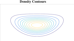
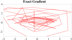
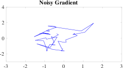
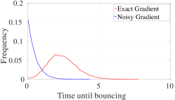
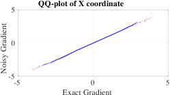
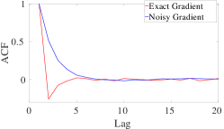
See Supp. Material A.2 for a proof sketch. Defining $\tilde{G}={\bf v}\cdot\nabla\tilde{U}({\bf w})$, the intensity of the inhomogeneous Poisson process $[\tilde{G}]_{+}$, which determines the time of the velocity bounce, now becomes stochastic, and the resulting point process is called a doubly stochastic, or Cox, process (Cox, 1955; Grandell, 1976). The effect of the gradient noise is to increase the average point process intensity, since $E\left[[\tilde{G}]_{+}\right]\geq\left[E[\tilde{G}]\right]_{+}$, from Jensen’s inequality. This leads to more frequent bounces and typically a slower mixing of the Markov process, as illustrated in Figure 1.

Many Cox processes are based on Poisson intensities obeying stochastic differential equations, or assume that the joint distribution at several ${\bf w}$’s has a non-trivial ${\bf w}$-dependent structure. Our case is different because we assume that ${\bf n}_{{\bf w}_{1}}$ and ${\bf n}_{{\bf w}_{2}}$ are independent even when ${\bf w}_{1}$ and ${\bf w}_{2}$ are infinitesimally close.

3.2 Sampling from Big Data posteriors

In a prototypical Bayesian setting, we have a prior $f({\bf w})$, i.i.d. data points $x_{i}$, and the negative log-posterior gradient is

$$\textstyle\nabla U({\bf w})=-\nabla\left[\log f({\bf w})+\underset{i=1}{\overset{N}{\sum}}\log p(x_{i}|{\bf w})\right]\,.$$ (8)

When $N$ is big we consider replacing the above gradient by the noisy approximation

$$\textstyle\nabla\tilde{U}({\bf w})=-\nabla\left[\log f({\bf w})+\frac{N}{n}\underset{i=1}{\overset{n}{\sum}}\log p(x_{r_{i}}|{\bf w})\right]\,,$$ (9)

where $n\ll N$ and the $n$ indices $\{r_{i}\}$ are sampled randomly without replacement. To sample from the posterior using the noisy gradient (9), we want to simulate the first arrival time in a doubly stochastic Poisson process with random intensity $[\tilde{G}(t)]_{+}$, where

$$\tilde{G}(t)={\bf v}\cdot\nabla\tilde{U}({\bf w}+{\bf v}t)\,.$$ (10)

Note that $\tilde{U}$ is a stochastic process, and noise independence for different ${\bf w}$’s implies that different $t$’s require independent mini-batches. Out of several methods to sample from (noisy) Poisson processes, the thinning method (Lewis & Shedler, 1979) is compatible with the noise independence assumption. This is a form of rejection sampling which proposes a first arrival time $t$, sampled from an inhomogeneous Poisson process with intensity $\lambda(t)$ such that $\lambda(t)\geq[\tilde{G}(t)]_{+}$ The particle moves a distance $t{\bf v}$, and accepts the proposal to bounce the velocity with probability $[\tilde{G}(t)]_{+}/\lambda(t)$. Note that this accept-reject step is different from the MH algorithm (Robert & Casella, 2013), since the particle always moves the distance $t{\bf v}$, and a rejection only affects the velocity bouncing. This can greatly improve the efficiency of the sampler. As in the noiseless case, one should in general also resample ${\bf v}$ occasionally, to ensure ergodicity (Bouchard-Côté et al., 2015), although in the examples we considered this was not empirically necessary, since the mini-batch noise serves to randomize the velocity sufficiently, preventing “non-ergodic” trajectories that do not explore the full space.

In some special cases one can derive a bound $\lambda(t)$ that always holds (Bouchard-Côté et al., 2015; Bierkens et al., 2017). But this is atypical, due to the dependence of $\tilde{G}(t)$ in (10) on the changing velocity ${\bf v}$ and the mini-batch noise. Even when such bounds do exist, they tend to be conservatively high, leading to an inefficient sampler with many rejected proposals (wasting many mini-batches of data) before accepting.

Instead, we propose below an adaptive approximate bound which achieves a bias-variance trade-off between the frequency of the bounce proposals and a controllable probability of bound violation.

4 Proposal from Local Regression

Our approach to an adaptive and tractable proposal intensity $\lambda(t)$ relies on a predictive model of $\tilde{G}$ based on previous observations; the key idea is to exploit the correlations between nearby $\tilde{G}$ values. The upper value of the resulting predictive confidence band can then be used as $\lambda(t)$, and this band is adaptively updated as more proposals are generated.

While there are many possibilities for such a predictive model, we found that a simple local linear model was very effective and computationally trivial. Consider then the linear regression of $m$ observed values $\tilde{G}_{i}\equiv\tilde{G}(t_{i})$ since the previous bounce,

$$\tilde{G}_{i}=\beta_{1}t_{i}+\beta_{0}+\varepsilon_{t_{i}}\qquad\varepsilon_{t_{i}}\sim N(0,c^{2}_{t_{i}})\,,$$ (11)

where $i=1,\ldots,m$ and the noise variance can be estimated from the mini-batch in (9) as

$$\textstyle c_{t}^{2}=\frac{N^{2}}{n}(1-\frac{n}{N})\textrm{Var}_{i}\left[{\bf v}\cdot\nabla\log p(x_{r_{i}}|{\bf w})\right]\,.$$ (12)

Here $\textrm{Var}_{i}$ denotes the sample variance of the mini-batch, and we included the finite population correction factor $(1-\frac{n}{N})$ because the indices $\{r_{i}\}$ are sampled without replacement. The Gaussian noise assumption in $\tilde{G}(t)$ in (11) is valid when the mini-batch is sufficiently large that we can appeal to a central limit theorem. (For heavy-tailed noise we could consider more robust estimators, but we do not pursue this direction here.)

Adding a Gaussian prior ${N}(\mu,\sigma^{2})$ to $\beta_{1}$, and defining $\mathbf{x}_{i}\equiv(1,t_{i})$, the log posterior of $\bm{\beta}=(\beta_{0},\beta_{1})^{T}$ is

$$\textstyle 2\log p(\bm{\beta}|\{t_{i},\tilde{G}_{i},c^{2}_{t_{i}}\}) = \textstyle-\underset{i=1}{\overset{m}{\sum}}\frac{(\tilde{G}_{i}-\mathbf{x}_{i}\cdot\bm{\beta})^{2}}{c_{t_{i}}^{2}}$$

$$- \textstyle\frac{(\beta_{1}-\mu)^{2}}{\sigma^{2}}+const.$$

Let $\hat{\bm{\beta}}$ and $\bm{\Sigma}$ be the mean and covariance of this distribution. Using these estimates, we obtain the predictive distribution $\hat{G}(t)$ for $\tilde{G}(t)$ for $t>t_{m}$,

$$\hat{G}(t)=\hat{\beta}_{1}t+\hat{\beta}_{0}+\eta_{t}\qquad\eta_{t}\sim N(0,\rho^{2}(t))$$ (13)

$$\text{where}\quad\rho^{2}(t)=\mathbf{x}\bm{\Sigma}\mathbf{x}^{T}+c^{2}_{t_{m}}$$ (14)

with ${\bf x}=(1,t)$. Note that as usual the noise variance is different in (11) and (13), since in (11) we are fitting observed pairs $\tilde{G}_{i},t_{i}$, while in (13) we are predicting the value of $\tilde{G}(t)$ and we include the uncertainty from the $\hat{\bm{\beta}}$ estimates. Also, for simplicity we extrapolate the observation noise to be the same as in the last mini-batch, $c^{2}_{t_{m}}$.

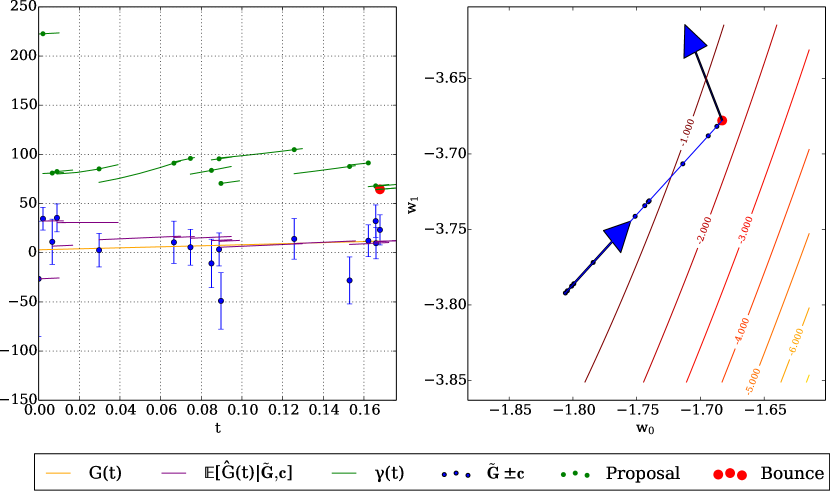
We can now construct a tractable approximate thinning proposal intensity by choosing a confidence band multiple $k$, and defining $\gamma(t)$ as a linear interpolation between selected points along the non-linear curve

$$\hat{\beta}_{1}t+\hat{\beta}_{0}+k\rho(t)\,.$$ (15)

The proposal intensity is now $\lambda(t)=[\gamma(t)]_{+}$, and sampling from an inhomogeneous Poisson process with piecewise linear rate $\lambda(t)$ can be done analytically using the inverse CDF method. When a bounce time is proposed at time $t$, the particle moves a distance $t{\bf v}$, a noisy observation $\tilde{G}(t)$ is made as in (10) and the bounce time is accepted with probability $\min(1,[\tilde{G}(t)]_{+}/\lambda(t))$. If the bounce is accepted, the velocity is reflected as in (6) (using $\tilde{U}$ instead of $U$), and the set of observed values is reinitialized with $(-\tilde{G}(t),c_{t})$, which are the values one would obtain from sampling the same mini-batch after the bounce, since ${\bf v}_{r}\cdot\tilde{U}=-{\bf v}\cdot\tilde{U}=-\tilde{G}(t)$. On the other hand, if the proposal is rejected, the observed $(\tilde{G}(t),c_{t})$ are added to the set of observed values. The hyperparameters $\mu,\sigma^{2}$ of the regression model can be learned by performing, after each bounce, a gradient ascent step on the marginal likelihood, $p(\{\tilde{G}_{i}\}|\mu,\sigma^{2})$; this gradient can be computed analytically and does not significantly impact the computational cost.

Figure 2: Thinning proposal intensity for bounce times from a linear regression predictive confidence interval applied to a two-dimensional logistic regression posterior with $N=1000,n=100$. Left: Starting from $t=0$, the piecewise linear intensity $\gamma(t)$ is used to propose bounce times (green points). As these proposals are rejected additional observations $\tilde{G}_{i}$ are made until a proposal is accepted (red point). The decrease in the slope of $\gamma(t)$ indicates the decreasing uncertainty in the estimated regression parameters as observations increase; note that the linear approximation for the true $G(t)$ is quite accurate here. Note also the reduced observation frequency at lower values of $G(t)$ indicating more efficient sampling than is achievable with the constant and much higher bounds used in (Bouchard-Côté et al., 2015; Bierkens et al., 2016), which were in the range $[10^{4},2*10^{4}]$ for this data. Right: The corresponding SBPS particle trajectory, with arrows indicating the initial velocity and the velocity after the bounce. The contours show the Laplace approximation of the log posterior.

The linear model for $\tilde{G}$ is good when the target distribution can be locally approximated by a Gaussian, since $\tilde{G}(t)$ in (10) is a projection of the derivative of the negative log posterior. When the posterior is highly non-Gaussian, a decaying weight can be used for more-distant observations, leading to a local regression; the scale of this decay can be fit again via stochastic gradient ascent on the predictive likelihood. We have also explored a Gaussian Process regression model, but it did not improve over the linear model in the cases we considered. In Supp. Material E we discuss a potential problem with our approach in the case of multimodal distributions, and propose a solution for such cases.

Finally, note that the directional derivative of $\tilde{U}({\bf w})$ needed in (10) can in many cases be computed at a cheaper cost (by a factor of $d=\dim({\bf w})$) than the full gradient. The latter is only needed when a bounce is accepted. This is in contrast to other gradient based samplers which require the full gradient at every step.

We dub this approach to BPS with noisy gradients Stochastic BPS (SBPS). See Supp. Material C for pseudocode. Figure 2 illustrates the evolution of these dynamic proposal intensities in a simple example. In Section 5, we consider a variant to SBPS, called pSBPS, that learns a diagonal preconditioning factor for the gradient, and leads to a more efficient exploration of the space when the posterior is highly anisotropic and roughly axis-aligned.

4.1 Bias in the Samples

The constant $k$ in (15) controls the tradeoff between bias from possible $[\tilde{G}(t)]_{+}/\lambda(t)>1$ cases and lower computational cost: higher $k$ leads to a more conservative (higher) proposal intensity and therefore a less-biased but more data-inefficient sampler. We present a bound on the Wasserstein distance between the exact and bias distributions in Supp. Material B, and explore this bias-variance tradeoff further in Supp. Material F. A quick bias diagnostic is the rate at which the bound is violated, i.e., cases with $[\tilde{G}(t)]_{+}/\lambda(t)>1$; if this rate is significantly higher than expected under the local linear regression model, then a different approach should be considered.

5 Preconditioned SBPS

Consider now the linear transformation ${\bf w}={\bf A}{\bf z}$ with an arbitrary square matrix ${\bf A}$. A distribution $p({\bf w})$ of interest can be expressed in terms of ${\bf z}$ as

$$p_{z}({\bf z})d{\bf z} = p({\bf w}({\bf z}))d{\bf w}=p({\bf A}{\bf z})|{\bf A}|d{\bf z}\,,$$ (16)

$$= \exp(-U_{z}({\bf z}))d{\bf z}\,.$$ (17)

The SBPS algorithm can be applied to the density $p_{z}({\bf z})$ using the gradients of $U({\bf w})$. For this note that $\nabla_{z}U_{z}({\bf z})={\bf A}\nabla_{w}U({\bf w})$. The Poisson intensity to compute bounces is $[G]_{+}$, with $G={\bf v}\cdot{\bf A}\nabla U({\bf w})$, and the velocity reflection is computed as

$${\bf v}_{r}={\bf v}-2\frac{({\bf v}\cdot{\bf A}\nabla U({\bf w})){\bf A}\nabla U({\bf w})}{||{\bf A}\nabla U({\bf w})||^{2}}\,.$$ (18)

The piecewise linear trajectory ${\bf z}_{t}={\bf z}_{0}+{\bf v}t$ becomes ${\bf w}_{t}={\bf w}_{0}+{\bf A}{\bf v}t$. The matrix ${\bf A}$ is called a preconditioner in the optimization literature, but can also be used in a sampling context to reduce anisotropy of posterior distributions; it is often the case that a good preconditioner is not known in advance but is instead learned adaptively (Duchi et al., 2011).

Figure 3: Effect of diagonal preconditioning on SBPS performance. Sampling is from the logistic regression posterior as described in Section 7.1 , with $d=20,N=1000,k=3,n=100$. The preconditioner parameters are $\beta=.99,\epsilon=10^{-4}$. Left: Contour plots of posterior log likelihood under the Laplace approximation. Center, right: ACF and trajectories in the direction of greatest covariance.

We use a diagonal preconditioner for simplicity. Denoting the $i$th component at the $j$th evaluation of the gradient by $g_{i}^{j}$, we define

$$\textstyle a_{i}^{j} = \textstyle\beta(g_{i}^{j})^{2}+(1-\beta)a_{i}^{j-1},$$ (19)

$$\textstyle\tilde{a}^{j} = \textstyle\frac{1}{d}\sum_{i=1}^{d}\frac{1}{\sqrt{a_{i}^{j}}+\epsilon}\,,$$ (20)

for some $0\leq\beta\leq 1,\epsilon\ll 1$. The preconditioner at iteration $j$ is defined as ${\bf A}^{j}=\textrm{Diag}\left(\frac{\tilde{a}^{j}}{\sqrt{a_{i}^{j}}+\epsilon}\right)$. This is the same preconditioner used in  (Li et al., 2016), up to the $\tilde{a}^{j}$ factor; the latter is needed here in order to prevent scaling of $\tilde{G}$.

As noted in (Li et al., 2016), a time dependent preconditioner requires adding a term proportional to $\frac{\partial{\bf A}^{j}}{\partial{\bf w}}$ to the gradient, yet this term is negligibly small and can be ignored when $\beta\approx 1$, since in this parameter regime the preconditioner changes slowly as a function of $j$ and thus of ${\bf w}$.

We call this preconditioned variant pSBPS. It performs favorably compared to SBPS when the posterior is anisotropic and axis-aligned, since we use a diagonal approximation of the Hessian in the preconditioner. See (Bierkens et al., 2017) for a related approach. As Figure 3 shows, pSBPS converges to the posterior mode faster than SBPS, and mixes faster in the direction of greatest covariance.

6 Related Works

\begin{overpic}[width=433.62pt]{lreg_d=20.pdf} \put(37.5,28.0){\includegraphics[scale={.5}]{comp_times.pdf}} \end{overpic}

Figure 4: Logistic regression posterior sampling, with $d=20,\,N=1000,\,k=3,\,n=100$ (best seen in color). Top Left: Negative Log Likelihood (NLL) per data point of samples from SBPS compared with SGLD (step sizes $0.01,0.1$), mSGNHT (step size $0.1$), lipSBPS and SS-ZZ (see text for definitions and references), all initialized at the same random positions. Also shown are the normalized NLL of the MAP estimator $NLL(\hat{{\bf w}})/N$ and the mean $\pm$ std. dev. of the Laplace approximation NLL (distributed as $\frac{1}{2N}\chi^{2}(d)+NLL(\hat{{\bf w}})/N$). The continuous samplers (SBPS, SS-ZZ, lipSBPS) were run to match the data cost of the discrete (SGLD, mSGNHT), and for their ACFs we discretized the continuous paths uniformly to obtain the same number of samples. Note that SBPS is the fastest to converge. Center/Right: Trajectories and ACFs in the directions of largest and smallest eigenvalues of the Laplace approximation inverse Hessian. The ACFs were calculated after burn-in, while the trajectory plots only show initial convergence. Inset: CPU runtime for 100 epochs, showing a $\times 35$ advantage of $n=100$ SBPS over $n=1$ SS-ZZ and lipSBPS

Biased Samplers: Many stochastic gradient samplers (e.g. (Welling & Teh, 2011)) can be formulated exactly using a Wiener process (Ma et al., 2015), but they are biased because (i) the Gaussian assumption in the noise may not hold for small mini-batches, and (ii) the MH correction to the time discretization is avoided or approximated. Recently, irreversible samplers have been studied in this context (Ma et al., 2016). Choosing the step size in these samplers can be quite challenging, as discussed below: too-large step sizes increase the bias, while too-small step sizes slow the mixing, and in generic high-dimensional examples there is no way to automatically tune the step size (though see (Giles et al., 2016) for recent progress). In contrast, the bias in SBPS, controlled by the constant $k$, does not come from time discretization, but from easy-to-track violations of the thinning bound when $[\tilde{G}(t)]_{+}/\lambda(t)>1$.

Exact non-BPS-like Samplers: Firefly MCMC (Maclaurin & Adams, 2014) augments the target distribution with one binary variable per data point, and yields unbiased samples while only querying a subset of data points at each iteration. But it needs distribution-dependent lower bounds on the likelihood and requires an initial full sweep of the data. Also mixing can be extremely slow (Quiroz et al., 2015; Bardenet et al., 2015), and all the dataset must be available for access all the time.

Two recent novel proposals are (Quiroz et al., 2016), based on debiased pseudolikelihood combined with variance reduction techniques, and (Pollock et al., 2016), based on quasi-stationary distributions. These methods are relatively more complex, and we have not yet systematically compared them against SBPS.

Exact BPS-like Samplers: Two subsampling variants of BPS which preserve the exact distribution are Local BPS (Bouchard-Côté et al., 2015), that needs a pre-processing step of computational cost $O(N\log N)$, and ZZ-SS (Bierkens et al., 2016). In these approaches, the requirement to preserve the distribution exactly leads to extremely conservative thinning bounds, which in turn yield a very slow exploration of the space, as we will see below. Also, the bounds need to be rederived for each new model (if possible at all), unlike SBPS which can be used for any differentiable posterior distribution.

7 Experiments

7.1 Logistic Regression

Although simpler MCMC methods perform well in Bayesian logistic regression (BLR) models (Chopin & Ridgway, 2015), we begin with this well-understood case for comparing SBPS against a few of the existing stochastic MCMC methods discussed in the previous section. To generate the data, we sampled the components of the true ${\bf w}\in\mathbb{R}^{d}$ from $\textrm{Unif}[-5,5]$ and $N$ data points $\{{\bf x}_{i}\}$ from a $d$-dimensional zero-mean Gaussian, with one component of the diagonal covariance set to 6 and all the rest to 1. Labels $\{y_{i}\}$ are drawn from $y_{i}\sim\textrm{Bern}(\sigma({\bf w}\cdot{\bf x}_{i}))$, where $\sigma(x)=1/(1+e^{x})$. In the regime $d\ll N$ the Laplace approximation holds fairly well, providing another good comparison method. Figure 4 shows results for $N=1000,d=20,k=3,n=100$.

We run comparisons against the biased stochastic samplers Stochastic Gradient Langevin Dynamics (SGLD) (Welling & Teh, 2011) and multivariate Stochastic Gradient Nose-Hoover Thermostat (mSGNHT) (Li et al., 2015) with fixed step sizes. As noted above, choosing optimal step sizes for these samplers is challenging. To allow SGLD and mSGNHT to perform best, we performed a scan to find the largest (fastest-mixing) step size that did not lead to overly large bias compared to the Laplace approximation. (Note, importantly, that this scan is expensive and is not possible in high-dimensional examples where the Laplace approximation does not hold - precisely the cases where MCMC methods are most valuable.) See Supp. Material E for details of this scan, which led to an optimal step size of $0.1$ for SGLD. Larger step sizes led to visible biases in the samples (not shown); we also show the results with step size $0.01$ for comparison to note that the results do depend sensitively on this parameter.

We also compare against ZZ-SS. Instead of Local BPS, we ran comparisons against an unbiased method we call lipSBPS (short for Lipshitz BPS), where the velocity bounces occur as first arrival events in a Poisson process with noisy intensity $[{\bf v}\cdot\nabla\tilde{U}({\bf w})]_{+}$ built from a noisy gradient (9) of minimal size $n=1$, and simulated with thinning using an exact upper bound derived in Supp. Material F. One can verify that the resulting stochastic process is identical to that of Local BPS. Our bound is higher than that used in (Bouchard-Côté et al., 2015) by up to a factor of 2, which results in up to twice as many bounce proposals. On the other hand, our bound can be computed in $O(N)$ time, does not require non-negative covariates, and can be used also for $n>1$. Again, we note that this lipSBPS method, like Local BPS and ZZ-SS, are not generally applicable because the derived bounds only apply in special cases.

The results of Figure 4 show that SBPS outperforms the optimally tuned SGLD and mSGNHT, and converges orders of magnitude faster than lipSBPS and ZZ-SS. While the latter two methods are unbiased, our results suggest that the small bias introduced by SBPS is worth the massive reduction in variance.

In Supp. Material F we explore the effects of the hyperparameters: $k$, $n$, and ${\bf v}$ refresh rate $\lambda_{r}$. The conclusion is that in this logistic example no manual hyperparameter tuning was required (in stark contrast to the careful step size tuning required for SGLD): the bias-controlling constant $k$ can be set in the range $k\in[3,5]$ (consistent with the tails of the Gaussian in the linear regression model) and the mini-batch size $n$ should be small, but large enough for the CLT to justify the noise term in (11); $n=100$ worked well, but the results were not sensitively dependent on $n$. For small values of $n$ the mini-batch variability provided sufficient velocity randomness that no additional velocity refreshes were necessary, so we did not have to tune $\lambda_{r}$ either.

The comparison to pSBPS shows an improvement in the rate of convergence to the posterior mode. The MAP estimator $\hat{{\bf w}}$ was calculated using SAG (Roux et al., 2012), and the Hessian was computed exactly.

7.2 Continuous Trajectory Sampling

Figure 5: Estimated mean of $f(w)=\sin((w-\hat{w}/r)$, under continuous and discrete samples, with different ratios $r/b,$ where $b\approx 2\times 10^{-2}$ is the average linear trajectory length. The posterior distribution and settings are as in Figure 4. Assuming the Laplace approximation holds, the expectation of $f$ is $0$. Left: For $r/b=1$ there is little difference between continuous or discrete samples. Center: For $r/b=10^{-2}$ the continuous mean converges faster than the discrete. Right: Expectation of the absolute value of the test function averaged over 5 runs of 1000 epochs, as a function of $r/b$. The advantage of the continuous expectation when this ratio is $r/b\ll 1$ is evident.

Figure 6: Neural network posterior sampling for a single hidden layer network trained on MNIST. $d=192,N=8340,n=500$. For SBPS $k=3$. The posterior is compared to an expensive Metropolis-Hastings run. SBPS shows comparable mixing to an appropriately chosen SGLD without the need for a scan over step sizes. As can be seen, a poor choice of SGLD step size can lead to slow mixing or bias in the narrow directions of the target

A unique feature of BPS-like samplers is that their output is a continuous trajectory. Given ${\bf w}_{0}$ and a set of $R$ velocities and bounce times $\{{\bf v}_{i},t_{i}\}$, the estimated expectation of a test function $f({\bf w})$ is

$$\left\langle f({\bf w})\right\rangle_{BPS}\equiv\frac{1}{T}\underset{i=0}{\overset{R-1}{\sum}}\underset{0}{\overset{t_{i}}{\int}}f({\bf w}_{i}+{\bf v}_{i}t)dt$$ (21)

where ${\bf w}_{i+1}={\bf w}_{i}+{\bf v}_{i}t_{i}$ and $T$ is the total particle travel time. For simple test functions this integral is analytic, while more generally it can be computed numerically with standard efficient one-dimensional quadrature methods. When $f({\bf w})$ varies across a characteristic length $r$ shorter than the average trajectory length $b$ of the linear segments, we intuitively expect the error in the estimate (21) to be smaller than in estimators based on discrete samples. Note that this advantage tends to diminish for higher SBPS noise, since the linear segments become shorter.

Figure 5 explores empirically this idea in a simple setting by comparing the value of the expectation of $f(w)=\sin((w-\hat{w})/r)$ under the posterior distribution of the logistic example considered above. Here $(w,\hat{w})$ are the first coordinates of the vectors $({\bf w},\hat{{\bf w}})$, $\hat{{\bf w}}$ is the MAP value, and $r$ the characteristic length of $f$. As expected, the error in the expectation is lower in the continuous case for $r/b<1$.

7.3 Neural Network Posterior Sampling

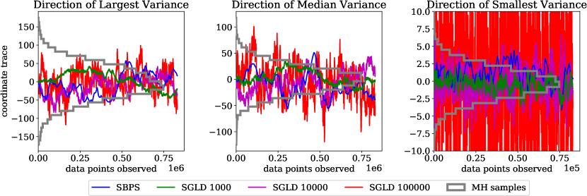
We considered a simple model of one hidden layer followed by a softmax. For Bayesian approaches to neural networks see (Neal, 2012; Gal, 2016). The likelihood was the standard cross entropy with an additional $L_{2}$ regularization term $L=-\underset{i=1}{\overset{N}{\sum}}\log(p_{i})+\frac{c}{2}\underset{j=1}{\overset{d}{\sum}}{\bf w}_{j}^{2}$ where $p_{i}$ is the probability of classifying the $i$th example correctly. $L$ was approximated via subsampling, and $c=0.001$. This architecture was trained on the MNIST dataset. A subset of the training set was preprocessed by downsampling the images to $7\times 7$, removing pixels that are 0 for all training examples and decreasing the number of digits to 4. The resulting training set size was $N=8340$. The resulting dimensionality of the posterior was $d=192$. Mini-batch size was $n=500$ for all methods. All weights were initialized at 0 and all methods were run for $10^{4}$ epochs. SBPS is compared with SGLD at different step sizes, and performance is comparable to SGLD with an appropriate step size without requiring an expensive scan over step sizes. Since the additional regularization term can lead to unbounded gradients of the log posterior $\nabla U({\bf w})$ one can no longer use the bounds derived for the Local BPS and ZZ-SS algorithms and thus they cannot be applied to this problem without further work. This is not the case for SBPS. The posterior is not Gaussian due to the likelihood terms and thus the Laplace approximation is not effective unless the posterior is dominated by the prior.

In order to assess the quality of the sampling, we compare the trajectories to a standard costly Metropolis-Hastings MCMC using a Gaussian with variance $0.2$ as the proposal distribution. This algorithm was run for $4*10^{5}$ epochs and the proposal acceptance rate was 0.43. Figure 6 shows samples in the directions of the largest, median and smallest variance of the empirical covariance matrix of the Metropolis-Hastings samples.

8 Conclusions

This paper introduced a non-reversible sampler that can be applied to big datasets by means of subsampling the data in each iteration. At the price of a small, controllable bias, it provides the benefits of (i) high mixing speed associated with non-reversibility, and (ii) continuous sample trajectories, with (iii) minimal hyperparameter tuning required, leading to state of the art performance and making it a convenient alternative to biased, difficult-to-tune MH-based stochastic samplers.

Stochastic Bouncy Particle Sampler

Supplementary Material

Appendix A Proof Sketch of Invariance under Noisy Gradients

In this section we start with a simple reformulation of the proof in (Bouchard-Côté et al., 2015) that the BPS Markov process leaves invariant the distribution $p({\bf w},{\bf v})=p({\bf w})p({\bf v})$ where

$$p({\bf w}) \propto e^{-U({\bf w})}\,,\qquad{\bf w}\in\mathbb{R}^{D}\,,$$ (A.1)

$$p({\bf v}) = \mathrm{Unif}[S^{D-1}]\,,$$ (A.2)

where $S^{D-1}$ is the $D$-dimensional one-sphere. This will set the stage for the noisy case considered next. For a more formal and detailed treatment of the BPS algorithm, including ergodicity, see (Bouchard-Côté et al., 2015). For simplicity, we do not include here the velocity refreshments, which do not change the proof.

The proof sketches below are presented using a discrete-time approach followed by letting $\Delta t\rightarrow 0$. We have found this approach more accessible for a machine learning audience. After submitting a preliminary version of this work to the arXiv, the preprint (Fearnhead et al., 2016) was submitted to the arXiv, which presents similar proofs of invariance by first deriving a general Fokker-Planck equation and then showing that the equation is satisfied both in noiseless and noisy cases.

A.1 Exact Gradient

To understand why the algorithm is correct, consider first the transition rule

$$({\bf w},{\bf v})_{t+\Delta t}=\left\{\begin{array}[]{ll}({\bf w}+{\bf v}\Delta t,{\bf v})&\textrm{with probability}\,\,1-\Delta t[G]_{+}\\ ({\bf w}+{\bf v}\Delta t,{\bf v}_{r})&\textrm{with probability}\,\,\Delta t[G]_{+}\end{array}\right.$$ (A.5)

where

$$[x]_{+}=\max(x,0)\,,$$ (A.6)

$$G={\bf v}\cdot\nabla U({\bf w})\,,$$ (A.7)

and

$${\bf v}_{r}={\bf v}-2\frac{({\bf v}\cdot\nabla U({\bf w}))\nabla U({\bf w})}{||\nabla U({\bf w})||^{2}}\,.$$ (A.8)

This rule acts on the probability density $p({\bf w},{\bf v})$ as,

$$p_{t+\Delta t}({\bf w},{\bf v}) = [p_{t+\Delta t}({\bf w},{\bf v})]_{d}+[p_{t+\Delta t}({\bf w},{\bf v})]_{r}\,.$$ (A.9)

The two terms in (A.9) correspond to the two ways to reach $({\bf w},{\bf v})$ at time $t+\Delta t$. First, we can start at $({\bf w}-{\bf v}\Delta t,{\bf v})$ at time $t$ and move a distance ${\bf v}\Delta t$ without bouncing. This occurs with probability $1-\Delta t[{\bf v}\cdot\nabla U]_{+}$, so we have

$$[p_{t+\Delta t}({\bf w},{\bf v})]_{d} = (1-\Delta t[{\bf v}\cdot\nabla U]_{+})p_{t}({\bf v})p_{t}({\bf w}-{\bf v}\Delta t)\,,$$ (A.10)

$$= (1-\Delta t[{\bf v}\cdot\nabla U]_{+})p_{t}({\bf v})(p_{t}({\bf w})-\Delta t{\bf v}\cdot\nabla p_{t}({\bf w})+O(\Delta t^{2}))\,,$$ (A.11)

$$= p_{t}({\bf v})p_{t}({\bf w})\left[1+\Delta t{\bf v}\cdot\nabla U-\Delta t[{\bf v}\cdot\nabla U]_{+}\right]+O(\Delta t^{2})\,,$$ (A.12)

where in (A.11) we did a Taylor expansion and in (A.12) we used (A.1).

The second term in (A.9) corresponds to being at $({\bf w}-{\bf v}_{r}\Delta t,{\bf v}_{r})$ at time $t$, moving ${\bf v}_{r}\Delta t$ and bouncing. This occurs with probability $\Delta t[{\bf v}_{r}\cdot\nabla U]_{+}=\Delta t[-{\bf v}\cdot\nabla U]_{+}$, so we have

$$[p_{t+\Delta t}({\bf w},{\bf v})]_{r} = \Delta t[-{\bf v}\cdot\nabla U]_{+}p_{t}({\bf w}-{\bf v}_{r}\Delta t,{\bf v}_{r})\,,$$ (A.13)

$$= \Delta t[-{\bf v}\cdot\nabla U]_{+}p_{t}({\bf w},{\bf v}_{r})+O(\Delta t^{2})\,,$$ (A.14)

where again we did a Taylor expansion in (A.13). Adding (A.12) and (A.14), and using

$$[{\bf v}\cdot\nabla U]_{+}-[-{\bf v}\cdot\nabla U]_{+}={\bf v}\cdot\nabla U\,,$$ (A.15)

equation (A.9) becomes

$$p_{t+\Delta t}({\bf w},{\bf v}) = p_{t}({\bf w},{\bf v})+O(\Delta t^{2})\,,$$ (A.16)

which implies that the distribution is stationary, $\frac{dp_{t}({\bf w},{\bf v})}{dt}=0$.

A.2 Noisy Gradient

Consider now a noisy gradient represented as

$$\nabla\tilde{U}({\bf w})=\nabla U({\bf w})+{\bf n}_{\bf w}\,,\qquad\qquad{\bf n}_{\bf w}\sim p({\bf n}_{\bf w}|{\bf w})\,,\quad\quad{\bf n}_{\bf w}\in{\mathbb{R}}^{D}\,,$$ (A.17)

where we assume that $p({\bf n}_{w}|{\bf w})$ has zero mean.

First note that the requirement that ${\bf n}_{\bf w}$ and ${\bf n}_{\bf w}^{\prime}$ are conditionally independent given ${\bf w}$ and ${\bf w}^{\prime}$, with ${\bf w}\neq{\bf w}^{\prime}$, is needed to preserve under the noise the Markov property of the sampler, which requires the bounce point process intensity to depend only on ${\bf w}$, and not the past history of the ${\bf w}$ trajectory.

Next we decompose the random vector ${\bf n}_{\bf w}$ into two orthogonal components,

$${\bf n}_{\bf w}=y{\bf v}+{\bf n}_{{\bf v}}\,,$$ (A.18)

with $y={\bf v}\cdot{\bf n}_{\bf w}$, and ${\bf n}_{{\bf v}}\cdot{\bf v}=0$. This induces a corresponding decomposition in the probability density as

$$d{\bf n}_{\bf w}p({\bf n}_{\bf w}|{\bf w})=dyd{\bf n}_{{\bf v}}p(y|{\bf w})p({\bf n}_{{\bf v}}|y,{\bf w},{\bf v})\,,$$ (A.19)

and note that from the assumption that $p({\bf n}_{\bf w}|{\bf w})$ has zero mean it follows that $p(y|{\bf w})$ has zero mean. The noisy projected gradient becomes

$${\bf v}\cdot\nabla U({\bf w})+y\,,\qquad y\sim p(y|{\bf w})\,.$$ (A.20)

To study the invariance of $p({\bf w},{\bf v})$ under the noisy BPS, let us consider again the decomposition (A.9) into straight and bounced infinitesimal trajectories. The probability that the particle is at $({\bf w}-{\bf v}\Delta t,{\bf v})$ at time $t$ and moves a distance ${\bf v}\Delta t$ without bouncing is the average of $1-\Delta t[{\bf v}\cdot\nabla U({\bf w})+y]_{+}$ over all the possible realizations of $y$, and is therefore given by

$$1-\Delta tP_{{\bf v}} \equiv 1-\Delta t\int_{-\infty}^{+\infty}\!\!\![{\bf v}\cdot\nabla U({\bf w})+y]_{+}p(y|{\bf w})dy\,,$$ (A.21)

$$= 1-\Delta t\int_{-{\bf v}\cdot\nabla U({\bf w})}^{+\infty}\!\!\!\,({\bf v}\cdot\nabla U({\bf w})+y)p(y|{\bf w})dy\,,$$ (A.22)

where the above expression defines $P_{{\bf v}}$. The first term of (A.9) is therefore

$$[p_{t+\Delta t}({\bf w},{\bf v})]_{d} = (1-\Delta tP_{{\bf v}})p({\bf w}-{\bf v}\Delta t,{\bf v})\,,$$

$$= p_{t}({\bf w},{\bf v})-\Delta t{\bf v}\cdot\nabla p_{t}({\bf w})p_{t}({\bf v})-\Delta tP_{{\bf v}}p_{t}({\bf w})p_{t}({\bf v})+O(\Delta t^{2})\,,$$

$$= p_{t}({\bf w})p_{t}({\bf v})[1+\Delta t{\bf v}\cdot\nabla U({\bf w})-\Delta tP_{{\bf v}}]+O(\Delta t^{2})\,,$$ (A.24)

similarly to (A.10)-(A.12).

The second term in (A.9) now has contributions from all those values $({\bf w}-\tilde{{\bf v}}_{r}\Delta t,\tilde{{\bf v}}_{r})$ at time $t$, such that a reflection of $\tilde{{\bf v}}_{r}$ with respect to a noisy $\nabla\tilde{U}({\bf w})$ gives ${\bf v}$. Such a $\tilde{{\bf v}}_{r}$ exists for every value of the noise vector ${\bf n}_{w}$, and is given by

$$\tilde{{\bf v}}_{r}={\bf v}-2\frac{({\bf v}\cdot\nabla\tilde{U}({\bf w}))\nabla\tilde{U}({\bf w})}{||\nabla\tilde{U}({\bf w})||^{2}}\,,$$ (A.25)

Therefore the second term in (A.9) contains contributions from all the possible realizations of ${\bf n}_{\bf w}$ and is

$$[p_{t+\Delta t}({\bf w},{\bf v})]_{r} = \Delta t\int_{{\mathbb{R}}^{D}}d{\bf n}_{\bf w}[\tilde{{\bf v}}_{r}\cdot\nabla\tilde{U}({\bf w})]_{+}p({\bf n}_{\bf w}|{\bf w})p_{t}({\bf w}-\tilde{{\bf v}}_{r}\Delta t,\tilde{{\bf v}}_{r})\,,$$

$$= \Delta tp_{t}({\bf w},\tilde{{\bf v}}_{r})\!\int_{-\infty}^{+\infty}\!\!\!\!\!\!dy\,p(y|{\bf w})[-{\bf v}\cdot\nabla U({\bf w})-y]_{+}\,,\times\int\!\!\!d{\bf n}_{{\bf v}}p({\bf n}_{{\bf v}}|y,{\bf w},{\bf v})+\,O(\Delta t^{2})\,,$$

$$= \Delta tP_{{\bf v}_{r}}p_{t}({\bf w},\tilde{{\bf v}}_{r})+O(\Delta t^{2})\,,$$ (A.27)

where we used $\tilde{{\bf v}}_{r}\cdot\nabla\tilde{U}({\bf w})=-{\bf v}\cdot\nabla U({\bf w})-y$, the measure decomposition (A.19), $\int\!\!\!d{\bf n}_{{\bf v}}p({\bf n}_{{\bf v}}|y,{\bf w},{\bf v})=1$ and defined

$$P_{{\bf v}_{r}} = \int^{-{\bf v}\cdot\nabla U({\bf w})}_{-\infty}\!\!\!dy\,(-{\bf v}\cdot\nabla U({\bf w})-y)p(y|{\bf w})\,.$$ (A.28)

Adding now (A.24) and (A.27), using $p(\tilde{{\bf v}}_{r})=p({\bf v})$ (since $p({\bf v})$ is uniform) and

$$P_{{\bf v}}-P_{{\bf v}_{r}}={\bf v}\cdot\nabla U({\bf w})\,,$$ (A.29)

which follows from (A.22) and (A.28), and the fact that $p(y|{\bf w})$ has zero mean, we get again the stationarity condition

$$p_{t+\Delta t}({\bf w},{\bf v}) = p_{t}({\bf w},{\bf v})+O(\Delta t^{2})\,.$$ (A.30)

Appendix B Biased Approximation

B.1 Biased bouncing rate

In the noiseless case, the velocity bounce is an event in a Poisson process with intensity $\lambda({\bf w})=[{\bf v}\cdot\nabla U({\bf w})]_{+}$ while in the noisy case, the average Poisson intensity is $\lambda_{n}({\bf w})=E_{y}[\lambda_{n}({\bf w},y)]$ where

$$\lambda_{n}({\bf w},y)=[{\bf v}\cdot\nabla U({\bf w})+y]_{+}\,.$$ (B.31)

When a thinning upper bound for $[{\bf v}\cdot\nabla U+y]_{+}$ is unknown and the distribution of $y$ is Gaussian with predicted variance $\rho^{2}$, our algorithm makes a bounce proposal from a Poisson process with intensity

$$\lambda_{\rho}({\bf w})=\hat{G}+k\rho({\bf w})\,,$$ (B.32)

where $\hat{G}$ is our estimate of ${\bf v}\cdot\nabla U({\bf w})$. At the proposed bounce point ${\bf w}$, we evaluate $\lambda_{n}({\bf w},y)$, and accept with probability $\min(\lambda_{n}({\bf w},y)/\lambda_{\rho}({\bf w}),1)$. The evaluation of $\lambda_{n}({\bf w},y)$ also provides an estimate $\sigma^{2}({\bf w})$ of the variance of $y$. Assuming $y$ is Gaussian, the probability of the bound violation event $1<\lambda_{n}/\lambda_{\rho}$, is

$$q({\bf w})=1-\Phi((\lambda_{\rho}({\bf w})-{\bf v}\cdot\nabla U({\bf w}))/\sigma({\bf w}))\,,$$ (B.33)

where $\Phi$ is the standard normal CDF. For a given $y$, the intensity is therefore,

$$\lambda_{b}({\bf w},y) = I_{[\frac{\lambda_{n}}{\lambda_{\rho}}<1]}\lambda_{n}({\bf w},y)+I_{[\frac{\lambda_{n}}{\lambda_{\rho}}>1]}\lambda_{\rho}({\bf w})$$ (B.34)

where $I_{[\cdot]}$ is the indicator function. Averaging over $y$ we get

$$\lambda_{b}({\bf w}) = E_{y}[\lambda_{b}({\bf w},y)]$$ (B.35)

$$= (1-q({\bf w}))E_{\lambda_{n}\leq\lambda_{\rho}}[\lambda_{n}({\bf w},y)]+q({\bf w})\lambda_{\rho}({\bf w})$$ (B.36)

If the probability of bound violation has a universal upper bound $q({\bf w})<q,\forall{\bf w}$, we assume

$$|\lambda_{b}({\bf w})-\lambda_{n}({\bf w})|\leq K_{q}=Cq+O(q^{2})$$ (B.37)

where $C$ is a constant.

B.2 Preliminaries

We are interested bounding the distance between the equilibrium distribution of the biased, noisy BPS process with mean intensity $\lambda_{b}({\bf w})$, and the exact, noisy process with mean intensity $\lambda_{n}({\bf w})$. We start with some preliminary results.

Wasserstein Distance and Kantorovich Duality

We will consider the Wasserstein distance, defined as

$$d_{\cal W}(p_{1},p_{2})=\sup_{f\in C_{L}}|E_{p_{1}}[f]-E_{p_{2}}[f]|\,,$$ (B.38)

where $C_{L}$ is the set of 1-Lipshitz continuous functions,

$$C_{L}=\{f:\mathbb{R}^{d}\rightarrow\mathbb{R}:|f(y)-f(x)|\leq|y-x|\}\,.$$ (B.39)

Given random variables ${\bf z}_{1}\sim p_{1},\,{\bf z}_{2}\sim p_{2}$, a coupling is a joint distribution $({\bf z}_{1},{\bf z}_{2})\sim p_{12}$ with marginals $p_{1}$ and $p_{2}$. The Kantorovich duality (Villani, 2008) asserts that

$$d_{\cal W}(p_{1},p_{2})=\inf_{p_{12}}E_{p_{12}}[|{\bf z}_{1}-{\bf z}_{2}|]\,.$$ (B.40)

Generators

To simplify the notation, let us define ${\bf z}=({\bf w},{\bf v})$, ${\bf z}_{r}=({\bf w},\tilde{{\bf v}}_{r})$. The infinitesimal generator of a stochastic process is defined as

$${\cal L}f({\bf z})=\lim_{\delta t\rightarrow 0}\frac{E[f({\bf z}_{t+\delta t})|{\bf z}_{t}={\bf z}]-f({\bf z})}{\delta t}\,,$$ (B.41)

and note that it satisfies

$$E[{\cal L}f] = \lim_{\delta t\rightarrow 0}\frac{\int d{\bf z}_{t+\delta t}d{\bf z}p({\bf z}_{t+\delta t}|{\bf z})p({\bf z})f({\bf z}_{t+\delta t})-E[f({\bf z})]}{\delta t}\,,$$ (B.42)

$$= \lim_{\delta t\rightarrow 0}\frac{\int d{\bf z}_{t+\delta t}p({\bf z}_{t+\delta t})f({\bf z}_{t+\delta t})-E[f({\bf z})]}{\delta t}\,,$$ (B.43)

$$= 0,$$ (B.44)

where the expectation is with respect to the distribution $p({\bf z})$ invariant under the stochastic process, and we used $\int d{\bf z}p({\bf z}_{t+\delta t}|{\bf z})p({\bf z})=p({\bf z}_{t+\delta t})$. In our case, the generator of a BPS process with intensity $\lambda_{n}({\bf w},y)$ is (Davis, 1984; Fearnhead et al., 2016)

$${\cal L}_{\lambda_{n}}f({\bf z})={\bf v}\cdot\nabla_{{\bf w}}f({\bf z})+E_{y}[\lambda_{n}({\bf w},y)(f({\bf z}_{r})-f({\bf z}))]$$ (B.45)

and similarly for $\lambda_{b}({\bf w})$.

Let us define

$$f_{\lambda}({\bf z},t)=E_{\lambda}[f({\bf z}_{t})|{\bf z}_{0}={\bf z}]\,,$$ (B.46)

where the expectation is with respect to the distribution of the stochastic process with intensity $\lambda$ at time $t$ and with a given initial condition. This expression satisfies the backward Kolmogorov equation

$$\frac{\partial f_{\lambda}({\bf z},t)}{\partial t} = {\cal L}_{\lambda}f_{\lambda}({\bf z},t)\,,$$ (B.47)

and also (Jacod & Shiryaev, 1987)

$$\lim_{t\rightarrow\infty}f_{\lambda}({\bf z},t)=E_{\lambda}[f]\,,$$ (B.48)

where the expectation $E_{\lambda}[\cdot]$ is with respect to the distribution invariant under the stochastic process with intensity $\lambda$.

Ergodicity

We assume that the random process defined by SBPS is polynomial ergodic (although see the recent (Deligiannidis et al., 2017)). In particular, we assume that two distributions started at reflected velocities $p_{\lambda_{n},t,{\bf z}}=p_{\lambda_{n}}({\bf z}_{t}|{\bf z}_{0}={\bf z}),\,p_{\lambda_{n},t,{\bf z}_{r}}=p_{\lambda_{n}}({\bf z}_{t}|{\bf z}_{0}={\bf z}_{r})$ converge as

$$d_{\cal W}(p_{\lambda_{n},t,{\bf z}},p_{\lambda_{n},t,{\bf z}_{r}})\leq\frac{C_{A}}{(\alpha+t)^{\beta}}$$ (B.49)

where $\alpha,\beta,C_{A}$ are constants.

Poisson Equation

Given a function $f({\bf z})$, we will consider below the Poisson equation

$${\cal L}_{\lambda}u_{f}({\bf z})=f({\bf z})-E_{\lambda}[f]\,.$$ (B.50)

We assume the existence of the solution

$$u_{f}({\bf z})=\int_{0}^{\infty}ds(E_{\lambda}[f]-f_{\lambda}({\bf z},s))\,,$$ (B.51)

where $f_{\lambda}({\bf z},s)$ was defined in (B.46). The fact that this expression solves (B.50) can be easily verified using (B.47), (B.48) and $f_{\lambda}({\bf z},0)=f({\bf z})$. For $f\in C_{L}$ (see (B.39) ), this solution satisfies

$$|u_{f}({\bf z})-u_{f}({\bf z}_{r})| = \left|\int_{0}^{\infty}ds(f_{\lambda}({\bf z},s)-f_{\lambda}({\bf z}_{r},s))\right|$$ (B.52)

$$\leq \int_{0}^{\infty}dsE_{\lambda}[{\bf z}_{s}-{\bf z}_{r,s}|]\,,\quad\textrm{using the Lipshitz property }$$ (B.53)

$$\leq \int_{0}^{\infty}ds\,d_{\cal W}(p_{\lambda,s,{\bf z}},p_{\lambda,s,{\bf z}_{r}})\,,\quad\textrm{using~{}(\ref{kantorovich}) }$$ (B.54)

$$\leq \frac{C_{A}}{(\beta+1)\alpha^{\beta+1}}\,,\quad\textrm{using the ergodicity assumption (\ref{ergo})}\,.$$ (B.55)

B.3 Distance Bound from Stein’s Method

We now prove a bound on the distance between the exact and biased distributions, using Stein’s method (Barbour, 1990; Ross, 2011; Stein et al., 1972), which was recently used for the related Zig-Zag process (Huggins & Zou, 2017).

$$d_{\cal W}(p_{\lambda_{n}},p_{\lambda_{b}}) = \sup_{f\in C_{L}}|E_{{\lambda_{n}}}[f]-E_{{\lambda_{b}}}[f]|\,,$$ (B.56)

$$= \sup_{f\in C_{L}}|E_{{\lambda_{n}}}[{\cal L}_{\lambda_{b}}u_{f}]|\,,\quad\textrm{using (\ref{poisson})}$$ (B.57)

$$= \sup_{f\in C_{L}}|E_{{\lambda_{n}}}[{\cal L}_{\lambda_{b}}u_{f}]-E_{{\lambda_{n}}}[{\cal L}_{\lambda_{n}}u_{f}]|\,,\quad\textrm{using (\ref{elfz})}$$ (B.58)

$$\leq \sup_{f\in C_{L}}E_{{\lambda_{n}}}[|({\cal L}_{\lambda_{b}}-{\cal L}_{\lambda_{n}})u_{f}|]\,.$$ (B.59)

Note that this last expression involves an integral over just one distribution, unlike the first expression (B.56). Inside the expectation we have, using (B.45),

$$({\cal L}_{\lambda_{n}}-{\cal L}_{\lambda_{b}})u_{f}({\bf z}) \leq |\lambda_{n}({\bf w})-\lambda_{b}({\bf w})|E_{y}[|u_{f}({\bf z}_{r})-u_{f}({\bf z})|]\,,$$ (B.60)

where the expectation over $y$ is because ${\bf z}_{r}=({\bf w},{\bf v}_{r})$ depends on the noise $y$ (see (A.25)). Using (B.37) and (B.55), we get finally

$$d_{\cal W}(p_{\lambda_{n}},p_{\lambda_{b}})\leq\frac{K_{q}C_{A}}{(\beta+1)\alpha^{\beta+1}}\,.$$ (B.61)

Interestingly, this bound depends on the mixing speed of the process generated by ${\cal L}_{\lambda_{n}}$ (see (B.49)), even though the distance is between two equilibrium distributions.

Appendix C SBPS algorithm

Algorithm 2 provides a description of the SBPS algorithm with a linear regression based thinning proposal intensity. We have omitted velocity refreshments for the sake of clarity. $\Delta t$ in the code below is the resolution of the piecewise linear proposal intensity, which should be smaller than the typical time between bounces. In all experiments a value of $\Delta t=.01$ was used.

Appendix D A Highly non-Gaussian Example

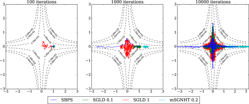
We explored a case of sampling from a Bayesian posterior where the Laplace approximations is not accurate. Figure 7 shows results for a highly non-log-concave 2D hyperboloid posterior, with data generated according to $y_{i}\sim\mathcal{N}(w_{0}^{*}w_{1}^{*},\sigma)$. After introducing a weak Gaussian prior, the resulting log posterior takes the form

$$L(w_{0},w_{1}|\{y_{i}\},\sigma)=\underset{i=1}{\overset{N}{\sum}}-\frac{(y_{i}-w_{0}w_{1})^{2}}{2\sigma^{2}}-\frac{c}{2}||w||_{2}^{2}\,.$$ (D.62)

This posterior was approximated by observing mini-batches of data as in the previous examples. The scaling symmetry that is manifest in the invariance of the likelihood with respect to $w_{0},w_{1}\rightarrow\lambda w_{0},\frac{w_{1}}{\lambda}$ leads to the highly non-Gaussian hyperboloid form. Similar symmetries are encountered in posteriors of deep neural networks with ReLU activation (Dinh et al., 2017). The parameters used were $N=1000,n=100,k=3,c=.0001,w_{0}^{*}=w_{1}^{*}=0,\sigma=1$. $\sigma$ was not learned.

Figure 7 shows comparisons with SGLD and mSGNHT, while Local BPS and SS-ZZ cannot be applied since there seems to be no simple exact upper bound for thinning in this case. Note that for the step sizes shown, both SGLD and mSGNHT deviate into low density regions while not mixing as well as SBPS. The smaller SGLD step size used does not deviate as much but exhibits even slower mixing.

Figure 7: Sample traces of SBPS, SGLD and mSGNHT sampling a highly non-Gaussian posterior. SBPS appears to explore the posterior more fully and avoids regions of low density as opposed to the large step size SGLD, leading to less bias.

Appendix E Sampling from Multimodal Targets

Our simple linear model for $G(t)$ (the projected gradient of the log posterior), appears to be sufficiently accurate even when the Laplace approximation is violated (as shown in the previous examples), but in some highly multimodal cases we have found this approximation to be insufficient.

In this section we present a slight modification of SBPS to sample from such targets as well. The potential troubles arise because in a multimodal target one may encounter situations where the measured $G(t)$ drop quickly between successive observations, leading to strong negative regression slopes. In our regression model, we get an interpolation (cf. equation (13)) leading to an upper bound of the form

$$\hat{\beta}_{1}t+\hat{\beta}_{0}+k\rho(t)$$ (E.63)

with $\hat{\beta}_{1}<0$. Since the leading order $t$ dependence in $\rho(t)$ is linear, if $k$ is too small the linear term in (E.63) may be negative. This will lead the sampler to propose long times between samples and thus enter low target density regions of the space.

In such cases, we propose to make additional auxiliary observations at times $\{t_{aux}\}$ along the current linear trajectory of the particle and update the linear bound accordingly before making the next proposal. On a large enough scale this procedure will make auxiliary observations $\tilde{G}>0$ leading to a positive slope in (E.63). This in turn will prevent the particle from entering low target density regions.

Note that these auxiliary observations can be performed with the same minibatch of data from the last bounce proposal. In principle, such strong negative slopes can occur even for a unimodal target if the subsampling noise is highly non-Gaussian, and this mechanism can also be used in those situations.

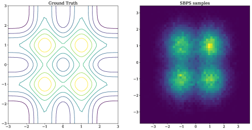
We illustrate this mechanism in a simple distribution defined as

$$L(w)=\sum_{i=1}^{N}\underset{k=1}{\overset{D}{\sum}}L_{i}(w_{k})+\textrm{const.}$$ (E.64)

where $w\in\mathbb{R}^{D}$ and

$$L_{i}(w_{k})=\log\left[e^{-\frac{(w_{k}-1-\mu_{k}^{i})^{2}}{2\sigma_{L}^{2}}}+e^{-\frac{(w_{k}+1-\mu_{D+k}^{i})^{2}}{2\sigma_{L}^{2}}}\right]$$ (E.65)

and each ${\mu^{i}_{k}}$ is drawn from $\mathcal{N}(0,\sigma_{\mu})$. This is a highly multimodal toy distribution. Although it does not come from a posterior distribution, it allows us to illustrate the proposed mechanism in a clean setting. Figure 8 shows results for $D=2$, $N=1000,\sigma_{L}=.25,\sigma_{\mu}=.01$ and mini-batch size $n=10$. We used $\{t_{aux}\}=\{10p\overline{t},p\in\mathbb{N}\}$ where $\overline{t}$ is the mean proposal time of all past proposals during the sampling process. While one can add multiple auxiliary points in this way, in practice we have found that one auxiliary point ($p=1$) is sufficient. Figure 8 shows that SBPS is able to correctly sample from the target while avoiding the issues posed by the multimodality of the distribution. We note that this modified mechanism does not affect the rest of the examples presented in this paper.

Figure 8: SBPS sampling from a highly multimodal target. As can be seen from the sample histogram on the right, SBPS manages to accurately capture the multimodal target. The results are from 1000 epochs of sampling from a dataset of size $N=1000$

Appendix F SGLD Step Size Scan

Figure 9: Per-data-point variance of the NLL in the logistic regression example of Section 7.1, using SGLD samples with step sizes of $10^{-i/2},i=0...9$. The samplers were initialized at the MAP. We select the biggest step size whose empirical variance is below that from the Laplace approximation, $\frac{d}{2N^{2}}$.

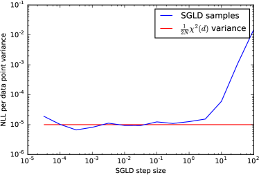
In the logistic regression example of Section 6.1, we compare SBPS with Stochastic Gradient Langevin Dynamics (SGLD) (Welling & Teh, 2011) with fixed step size. A natural question is how to choose an appropriate step size that ensures the fastest possible mixing without introducing an unacceptable amount of bias. Our criterion was to pick the biggest possible (i.e., fastest-mixing) step size such that the resulting variance of the per-data-point Negative Log Likelihood (NLL) coincides with that of the Laplace approximation. The latter gives a per-data-point NLL distribution of $\frac{1}{2N}\chi^{2}(d)+NLL_{\hat{{\bf w}}}/N$ where $\hat{{\bf w}}$ is the MAP estimator (Bickel & Doksum, 2015). The results of this parameter scan are shown in Figure 9 and suggest a step size of $0.1$.

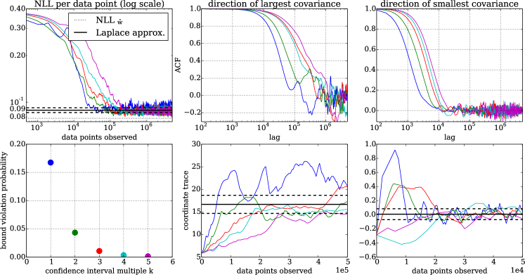
Appendix G The effect of the SBPS hyperparameters

In this section we explore, in the logistic regression example of Section 6.1, the effect of two hyperparameters that control the behavior of SBPS: the mini-batch size $n$, and the width $k$ of the upper confidence band. A third hyperparameter is the rate of velocity refreshments, shown in (Bouchard-Côté et al., 2015) to be necessary in general to prove ergodicity. But, as mentioned in Section 3, in the examples we considered the mini-batch noise was enough to sufficiently randomize possible non-mixing trajectories, so we could safely set this parameter to a very low value.

G.1 Mini-batch size $n$

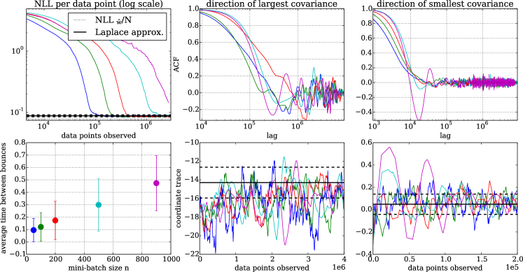
Figure 10 shows an exploration of different values of the mini-batch size $n$. Low values for $n$ lead to high noise for $\tilde{G}$. This in turn yields higher values for the proposal intensity $\gamma(t)$, which leads to shorter linear trajectories between bounce proposals. This is consistent with the results of Figure 10 that show a linear relation between $n$ (i.e. computational cost per bounce proposal) and the average travel time between bounces. The autocorrelation functions (ACFs) were computed from discrete samples obtained by running SBPS with different $n$’s such that the total data cost was the same for all cases, and then discretizing the continuous paths into equal numbers of uniformly spaced samples. As shown, these cost adjusted ACFs are quite similar. On the other hand, the upper-left panel, shows that lower values of $n$ have faster convergence to equilibrium, suggesting that low $n$ should be preferred. But this should be contrasted with the fact that shorter linear trajectories increase the variance of expectations over rapidly changing functions, as discussed in Section 6.3.

Figure 10: Effect of mini-batch sizes $n$ in the logistic regression example of Section 6.1. Mini-batch sizes were $50,100,200,500,900$. Top Left: Average per-data-point NLL over 5 runs. Note that smaller $n$ lead to faster convergence to a region of low NLL. Lower Left: Estimated average time between particle bounces. Center/Right: ACF and trajectories from a single run, in the directions of smallest and biggest covariance. The x axis was chosen differently for the trajectory plots for clarity.

Figure 11: Effect of upper band size $k$ in the logistic regression example of Section 6.1, run with mini-batch size $n=100$. Bottom Left: Rate of upper bound violations as a function of $k$; the same colors are used in the other plots. Top Left: NLL per data point for samples of SBPS with different k values. Center/Right: ACF and trajectories in the directions of smallest and biggest covariance. Note that smaller $k$ leads to faster convergence and mixing but increased bias, as visible in the coordinate trace in the direction of biggest covariance. The x axis was chosen differently for the trajectory plots for clarity.

G.2 Upper-band width $k$

Figure 11 shows an exploration of different values of $k$, the height of the proposal intensity above the estimator mean, in units of predictive standard deviation (see in Eq.(12) in main text). It therefore controls the trade-off between a regime, at low $k$, of faster mixing and high bias from violations of the thinning upper bound ($[\tilde{G}(t)]_{+}/\lambda(t)>1$), and another regime, high $k$, of low bias and high variance from slower mixing. As expected, the probability of bound violation decreases monotonically with $k$, as seen in the bottom left panel of Figure 11.

Appendix H Upper Bounds for Logistic Regression

In the case of logistic regression with data $(y_{i},{\bf x}_{i})$ the estimator of $\nabla_{\bf w}U({\bf w})$ from a mini-batch of size $n$ is

$$\nabla_{\bf w}\tilde{U}({\bf w})=\frac{N}{n}\sum_{i=1}^{n}{\bf x}_{i}(\sigma({\bf w}\cdot{\bf x}_{i})-y_{i})\,.$$ (H.66)

A simple bound on $\tilde{G}(t)$ is therefore given by

$$\tilde{G}(t) \leq\frac{N}{n}|\sum_{i=1}^{n}(\mathbf{v}\cdot{\bf x}_{i})(\sigma({\bf w}\cdot{\bf x}_{i})-y_{i})|\,,$$ (H.67)

$$\leq\frac{N}{n}\sum_{i=1}^{n}||\mathbf{v}||_{2}||(\sigma({\bf w}\cdot{\bf x}_{i})-y_{i}){\bf x}_{i}||_{2}\,,$$ (H.68)

$$\leq\frac{N}{n}\sum_{i=1}^{n}||x_{i}||_{2}\,,$$ (H.69)

$$\leq\sqrt{d}N\max_{i,j}|x_{ij}|\,.$$ (H.70)

This is a particular case of a bound derived in (Bierkens et al., 2017). Compared to the bound proposed in (Bouchard-Côté et al., 2015), this bound is more conservative but cheaper to compute and does not require non-negative covariates. It similarly scales like $N$ and when the data used in the experiments was modified so that the covariates were non-negative the bounds differed by a factor lower than 2.

References

- Ahn et al. (2012) Ahn, Sungjin, Korattikara, Anoop, and Welling, Max. Bayesian posterior sampling via stochastic gradient fisher scoring. ICML, 2012.
- Barbour (1990) Barbour, Andrew D. Stein’s method for diffusion approximations. Probability theory and related fields, 84(3):297–322, 1990.
- Bardenet et al. (2014) Bardenet, Rémi, Doucet, Arnaud, and Holmes, Chris. Towards scaling up Markov chain Monte Carlo: an adaptive subsampling approach. In ICML, pp. 405–413, 2014.
- Bardenet et al. (2015) Bardenet, Rémi, Doucet, Arnaud, and Holmes, Chris. On Markov chain Monte Carlo methods for tall data. arXiv:1505.02827, 2015.
- Bickel & Doksum (2015) Bickel, Peter J and Doksum, Kjell A. Mathematical Statistics: Basic Ideas and Selected Topics, volume I, volume 117. CRC Press, 2015.
- Bierkens & Roberts (2015) Bierkens, Joris and Roberts, Gareth. A piecewise deterministic scaling limit of Lifted Metropolis-Hastings in the Curie-Weiss model. arXiv:1509.00302, 2015.
- Bierkens et al. (2016) Bierkens, Joris, Fearnhead, Paul, and Roberts, Gareth. The Zig-Zag Process and Super-Efficient Sampling for Bayesian Analysis of Big Data. arXiv preprint arXiv:1607.03188, 2016.
- Bierkens et al. (2017) Bierkens, Joris, Bouchard-Côté, Alexandre, Doucet, Arnaud, Duncan, Andrew B, Fearnhead, Paul, Roberts, Gareth, and Vollmer, Sebastian J. Piecewise Deterministic Markov Processes for Scalable Monte Carlo on Restricted Domains. arXiv preprint arXiv:1701.04244, 2017.
- Bouchard-Côté et al. (2015) Bouchard-Côté, Alexandre, Vollmer, Sebastian J, and Doucet, Arnaud. The Bouncy Particle Sampler: A Non-Reversible Rejection-Free Markov Chain Monte Carlo Method. arXiv:1510.02451, 2015.
- Chen et al. (2014) Chen, Tianqi, Fox, Emily B, and Guestrin, Carlos. Stochastic gradient HMC. In ICML, pp. 1683—1691, 2014.
- Chopin & Ridgway (2015) Chopin, Nicolas and Ridgway, James. Leave Pima Indians alone: binary regression as a benchmark for Bayesian computation. arXiv preprint arXiv:1506.08640, 2015.
- Cox (1955) Cox, David R. Some statistical methods connected with series of events. J. Royal Stat. Soc., Series B (Methodological), pp. 129–164, 1955.
- Davis (1984) Davis, Mark HA. Piecewise-deterministic Markov processes: A general class of non-diffusion stochastic models. J. Royal Stat. Soc., Series B (Methodological), pp. 353–388, 1984.
- Deligiannidis et al. (2017) Deligiannidis, George, Bouchard-Côté, Alexandre, and Doucet, Arnaud. Exponential Ergodicity of the Bouncy Particle Sampler. arXiv preprint arXiv:1705.04579, 2017.
- Ding et al. (2014) Ding, Nan, Fang, Youhan, Babbush, Ryan, Chen, Changyou, Skeel, Robert D, and Neven, Hartmut. Bayesian sampling using stochastic gradient thermostats. In NIPS, pp. 3203–3211, 2014.
- Dinh et al. (2017) Dinh, Laurent, Pascanu, Razvan, Bengio, Samy, and Bengio, Yoshua. Sharp minima can generalize for deep nets. arXiv preprint arXiv:1703.04933, 2017.
- Duchi et al. (2011) Duchi, John, Hazan, Elad, and Singer, Yoram. Adaptive subgradient methods for online learning and stochastic optimization. Journal of Machine Learning Research, 12(Jul):2121–2159, 2011.
- Dufour et al. (2015) Dufour, François, Zhang, Huilong, et al. Numerical Methods for Simulation and Optimization of Piecewise Deterministic Markov Processes. John Wiley & Sons, 2015.
- Fearnhead et al. (2016) Fearnhead, Paul, Bierkens, Joris, Pollock, Murray, and Roberts, Gareth O. Piecewise Deterministic Markov Processes for Continuous-Time Monte Carlo. arXiv preprint arXiv:1611.07873, 2016.
- Gal (2016) Gal, Yarin. Uncertainty in Deep Learning (Cambridge PhD Thesis). 2016.
- Giles et al. (2016) Giles, Mike, Nagapetyan, Tigran, Szpruch, Lukasz, Vollmer, Sebastian, and Zygalakis, Konstantinos. Multilevel Monte Carlo for Scalable Bayesian Computations. arXiv preprint arXiv:1609.06144, 2016.
- Grandell (1976) Grandell, Jan. Doubly stochastic Poisson processes. Springer, 1976.
- Huggins & Zou (2017) Huggins, Jonathan H and Zou, James. Quantifying the accuracy of approximate diffusions and Markov chains. In AISTATS, 2017.
- Jacod & Shiryaev (1987) Jacod, J. and Shiryaev, A.N. Limit Theorems for Stochastic Processes. Grundlehren der mathematischen Wissenschaften in Einzeldarstellungen. Springer-Verlag, 1987. ISBN 9783540178828.
- Korattikara et al. (2013) Korattikara, Anoop, Chen, Yutian, and Welling, Max. Austerity in MCMC land: Cutting the Metropolis-Hastings budget. arXiv:1304.5299, 2013.
- Lewis & Shedler (1979) Lewis, Peter A and Shedler, Gerald S. Simulation of nonhomogeneous Poisson processes by thinning. Naval Research Logistics Quarterly, 26(3):403–413, 1979.
- Li et al. (2015) Li, Chunyuan, Chen, Changyou, Fan, Kai, and Carin, Lawrence. High-Order Stochastic Gradient Thermostats for Bayesian Learning of Deep Models. arXiv preprint arXiv:1512.07662, 2015.
- Li et al. (2016) Li, Chunyuan, Chen, Changyou, Carlson, David, and Carin, Lawrence. Preconditioned stochastic gradient langevin dynamics for deep neural networks. AAAI, 2016.
- Ma et al. (2015) Ma, Yi-An, Chen, Tianqi, and Fox, Emily. A complete recipe for stochastic gradient MCMC. In NIPS, pp. 2899–2907, 2015.
- Ma et al. (2016) Ma, Yi-An, Chen, Tianqi, Wu, Lei, and Fox, Emily B. A Unifying Framework for Devising Efficient and Irreversible MCMC Samplers. arXiv preprint arXiv:1608.05973, 2016.
- Maclaurin & Adams (2014) Maclaurin, Dougal and Adams, Ryan P. Firefly Monte Carlo: Exact MCMC with subsets of data. arXiv:1403.5693, 2014.
- Monmarché (2014) Monmarché, Pierre. Piecewise deterministic simulated annealing. arXiv preprint arXiv:1410.1656, 2014.
- Neal (2004) Neal, Radford M. Improving asymptotic variance of MCMC estimators: Non-reversible chains are better. arXiv preprint math/0407281, 2004.
- Neal (2012) Neal, Radford M. Bayesian learning for neural networks, volume 118. Springer Science & Business Media, 2012.
- Patterson & Teh (2013) Patterson, Sam and Teh, Yee Whye. Stochastic gradient Riemannian Langevin dynamics on the probability simplex. In NIPS, pp. 3102–3110, 2013.
- Peters & de With (2012) Peters, EAJF and de With, G. Rejection-free Monte Carlo sampling for general potentials. Phys. Rev. E, 85(2):026703, 2012.
- Pollock et al. (2016) Pollock, Murray, Fearnhead, Paul, Johansen, Adam M, and Roberts, Gareth O. The Scalable Langevin Exact Algorithm: Bayesian Inference for Big Data. arXiv preprint arXiv:1609.03436, 2016.
- Quiroz et al. (2015) Quiroz, Matias, Villani, Mattias, and Kohn, Robert. Speeding up MCMC by efficient data subsampling. Riksbank Research Paper Series, (121), 2015.
- Quiroz et al. (2016) Quiroz, Matias, Villani, Mattias, and Kohn, Robert. Exact Subsampling MCMC. arXiv:1603.08232, 2016.
- Robert & Casella (2013) Robert, Christian and Casella, George. Monte Carlo statistical methods. Springer Science & Business Media, 2013.
- Roberts et al. (2004) Roberts, Gareth O, Rosenthal, Jeffrey S, et al. General state space markov chains and mcmc algorithms. Probability Surveys, 1:20–71, 2004.
- Ross (2011) Ross, Nathan. Fundamentals of Stein’s method. Probab. Surv, 8:210–293, 2011.
- Roux et al. (2012) Roux, Nicolas L, Schmidt, Mark, and Bach, Francis R. A stochastic gradient method with an exponential convergence rate for finite training sets. In Advances in Neural Information Processing Systems, pp. 2663–2671, 2012.
- Stein et al. (1972) Stein, Charles et al. A bound for the error in the normal approximation to the distribution of a sum of dependent random variables. In Proceedings of the Sixth Berkeley Symposium on Mathematical Statistics and Probability, Volume 2: Probability Theory. The Regents of the University of California, 1972.
- Villani (2008) Villani, Cédric. Optimal transport: old and new, volume 338. Springer Science & Business Media, 2008.
- Vucelja (2014) Vucelja, Marija. Lifting–A Nonreversible MCMC Algorithm. arXiv:1412.8762, 2014.
- Welling & Teh (2011) Welling, Max and Teh, Yee W. Bayesian learning via stochastic gradient Langevin dynamics. In ICML, pp. 681–688, 2011.