An invariance principle for sums and record times of regularly varying stationary sequences

Abstract

We prove a sequence of limiting results about weakly dependent stationary and regularly varying stochastic processes in discrete time. After deducing the limiting distribution for individual clusters of extremes, we present a new type of point process convergence theorem. It is designed to preserve the entire information about the temporal ordering of observations which is typically lost in the limit after time scaling. By going beyond the existing asymptotic theory, we are able to prove a new functional limit theorem. Its assumptions are satisfied by a wide class of applied time series models, for which standard limiting theory in the space $D$ of càdlàg functions does not apply.

To describe the limit of partial sums in this more general setting, we use the space $E$ of so–called decorated càdlàg functions. We also study the running maximum of partial sums for which a corresponding functional theorem can be still expressed in the familiar setting of space $D$.

We further apply our method to analyze record times in a sequence of dependent stationary observations, even when their marginal distribution is not necessarily regularly varying. Under certain restrictions on dependence among the observations, we show that the record times after scaling converge to a relatively simple compound scale invariant Poisson process.

Keywords: point process regular variation invariance principle functional limit theorem record times

1 Introduction

Donsker–type functional limit theorems represent one of the key developments in probability theory. They express invariance principles for rescaled random walks of the form

$$S_{\lfloor nt\rfloor}=X_{1}+\cdots+X_{\lfloor nt\rfloor}\,,\quad t\in[0,1]\,.$$ (1.1)

Many extension of the original invariance principle exist, most notably allowing dependence between the steps $X_{i}$, or showing, like Skorohod did, that non–Gaussian limits are possible if the steps $X_{i}$ have infinite variance. For a survey of invariance principles in the case of dependent variables in the domain of attraction of the Gaussian law, we refer to Merlevède et al., (2006), see also Bradley, (2007) for a thorough survey of mixing conditions. In the case of a non–Gaussian limit, the limit of the processes $(S_{\lfloor nt\rfloor})_{t\in[0,1]}$ is not a continuous process in general. Hence, the limiting theorems of this type are placed in the space of càdlàg functions denoted by $D([0,1])$ under one of the Skorohod topologies. The topology denoted by $J_{1}$ is the most widely used (often implicitely) and suitable for i.i.d. steps, but over the years many theorems involving dependent steps have been shown using other Skorohod topologies. Even in the case of a simple $m$–dependent linear process from a regularly varying distribution, it is known that the limiting theorem cannot be shown in the standard $J_{1}$ topology, see Avram and Taqqu Avram and Taqqu, (1992). Moreover, there are examples of such processes for which none of the Skorohod topologies work, see Section 4.

However, as we found out, for all those processes and many other stochastic models relevant in applications, random walks do converge, but their limit exists in an entirely different space. To describe the elements of such a space we use the concept of decorated càdlàg functions and denote the corresponding space by $E([0,1])$, following Whitt Whitt, (2002). See Section 4. Presentation of this new type of limit theorem is the main goal of our article. For the statement of our main result see Theorem 4.5 in Section 4. As a related goal we also study the running maximum of the random walk $S_{\lfloor nt\rfloor}$ for which, due to monotonicity, the limiting theorem can still be expressed in the familiar space $D([0,1])$.

Our main analytical tool is the limit theory for point processes in a certain nonlocally compact space which is designed to preserve the order of the observations as we rescale time to interval $[0,1]$ as in (1.1). Observe that due to this scaling, successive observations collapse in the limit to the same time instance. As the first result in this context, we prove in Section 2 a limit theorem related to large deviations results of the type shown recently by Mikosch and Wintenberger, (2016) (cf. also Hult and Samorodnitsky, (2010)) and offer an alternative probabilistic interpretation of these results. Using our setup, we can group successive observations in the sequence $\{X_{i},\,i=1,\ldots,n\}$, in nonoverlapping clusters of increasing size to define a point process which completely preserves the information about the order among the observations. This allows us to show in a rather straightforward manner that so constructed empirical point processes converge in distribution towards a Poisson point process on an appropriate state space. The corresponding theorem could be arguably considered as the key result of the paper. It motivates all the theorems in the later sections and extends point process limit theorems in Davis and Hsing, (1995) and Basrak et al., (2012), see Section 3.

Additionally, our method allows for the analysis of records and record times in the sequence of dependent stationary observations $X_{i}$. By a classical result of Rényi, the number of records among first $n$ iid observations from a continuous distribution grows logarithmically with $n$. Moreover it is known (see e.g. Resnick, (1987)) that record times rescaled by $n$ tend to the so–called scale invariant Poisson process, which plays a fundamental role in several areas of probability, see Arratia, (1998). For a stationary sequence with an arbitrary continuous marginal distribution, we show that the record times converge to a relatively simple compound Poisson process under certain restrictions on dependence. This form of the limit reflects the fact that for dependent sequences records tend to come in clusters, as one typically observes in many natural situations. This is the content of Section 5. Finally, proofs of certain technical auxiliary results are postponed to Section 6. In the rest of the introduction, we formally present the main ingredients of our model.

We now introduce our main assumptions and notation. Let $\|\cdot\|$ denote an arbitrary norm on $\mathbb{R}^{d}$ and let $\mathbb{S}^{d-1}$ be the corresponding unit sphere. Recall that a $d$-dimensional random vector $\boldsymbol{X}$ is regularly varying with index $\alpha>0$ if there exists a random vector $\boldsymbol{\Theta}\in\mathbb{S}^{d-1}$ such that

$$\frac{1}{\mathbb{P}(\|\boldsymbol{X}\|>x)}\mathbb{P}(\|\boldsymbol{X}\|>ux,\boldsymbol{X}/\|\boldsymbol{X}\|\in\cdot)\Rightarrow u^{-\alpha}\mathbb{P}(\boldsymbol{\Theta}\in\cdot),$$ (1.2)

for every $u>0$ as $x\to\infty$, where $\Rightarrow$ denotes the weak convergence of measures, here on $\mathbb{S}^{d-1}$. An $\mathbb{R}^{d}$-valued time series $\{X_{t},t\in\mathbb{Z}\}$ is regularly varying if all the finite-dimensional vectors $(X_{k},\dots,X_{l})$, $k\leq l\in\mathbb{Z}$ are regularly varying, see Davis and Hsing, (1995) for instance. We will consider a stationary regularly varying process $\{X_{t},t\in\mathbb{Z}\}$. The regular variation of the marginal distribution implies that there exists a sequence $\{a_{n}\}$ which for all $x>0$ satisfies

$$n\mathbb{P}(\|X_{0}\|>a_{n}x)\to x^{-\alpha}\;.$$ (1.3)

If $d=1$, it is known that

$$n\mathbb{P}(X_{0}/a_{n}\in\cdot)\stackrel{{\scriptstyle v}}{{\longrightarrow}}\mu\;,$$ (1.4)

where $\stackrel{{\scriptstyle v}}{{\longrightarrow}}$ denotes vague convergence on $\mathbb{R}\setminus\{0\}$ with the measure $\mu$ on $\mathbb{R}\setminus\{0\}$ given by

$$\mu(dy)=p\alpha y^{-\alpha-1}\mathbbm{1}_{(0,\infty)}(y)\mathrm{d}y+(1-p)\alpha(-y)^{-\alpha-1}\mathbbm{1}_{(-\infty,0)}(y)\mathrm{d}y$$ (1.5)

for some $p\in[0,1]$.

According to Basrak and Segers, (2009), the regular variation of the stationary sequence $\{X_{t},t\in\mathbb{Z}\}$ is equivalent to the existence of an $\mathbb{R}^{d}$ valued time series $\{Y_{t},t\in\mathbb{Z}\}$ called the tail process which satisfies $\mathbb{P}(\|Y_{0}\|>y)=y^{-\alpha}$ for $y\geq 1$ and, as $x\to\infty$,

$$\left(\{x^{-1}X_{t},t\in\mathbb{Z}\}\,\big{|}\,\|X_{0}\|>x\right)\stackrel{{\scriptstyle\mathrm{fi.di.}}}{{\longrightarrow}}\{Y_{t},t\in\mathbb{Z}\}\;,$$ (1.6)

where $\stackrel{{\scriptstyle\mathrm{fi.di.}}}{{\longrightarrow}}$ denotes convergence of finite-dimensional distributions. Moreover, the so-called spectral tail process $\{\Theta_{t},t\in\mathbb{Z}\}$, defined by $\Theta_{t}=Y_{t}/\|Y_{0}\|$, $t\in\mathbb{Z}$, turns out to be independent of $\|Y_{0}\|$ and satisfies

$$\left(\{|X_{0}|^{-1}X_{t},t\in\mathbb{Z}\}\,\big{|}\,\|X_{0}\|>x\right)\stackrel{{\scriptstyle\mathrm{fi.di.}}}{{\longrightarrow}}\{\Theta_{t},t\in\mathbb{Z}\}\;,$$ (1.7)

as $x\to\infty$. If $d=1$, it follows that $p$ from (1.5) satisfies $p=\mathbb{P}(\Theta_{0}=1)=1-\mathbb{P}(\Theta_{0}=-1)$.

We will often assume in addition that the following condition, referred to as the anticlustering or finite mean cluster length condition, holds.

Assumption 1.1.

There exists a sequence of integers $(r_{n})_{n\in\mathbb{N}}$ such that $\lim_{n\to\infty}r_{n}=\lim_{n\to\infty}n/r_{n}=\infty$ and for every $u>0$,

$$\lim_{m\to\infty}\limsup_{n\to\infty}\mathbb{P}\biggl{(}\max_{m\leq|i|\leq r_{n}}\|X_{i}\|>a_{n}u\,\bigg{|}\,\|X_{0}\|>a_{n}u\biggr{)}=0\;.$$ (1.8)

There are many time series satisfying the conditions above including several nonlinear models like stochastic volatility or GARCH (see (Mikosch and Wintenberger,, 2013, Section 4.4)).

In the sequel, an important role will be played by the quantity $\theta$ defined by

$$\theta=\mathbb{P}\left(\sup_{t\geq 1}\|Y_{t}\|\leq 1\right)\;.$$ (1.9)

It was shown in (Basrak and Segers,, 2009, Proposition 4.2) that Assumption 1.1 implies that $\theta>0$.

2 Asymptotics of clusters

Let $l_{0}$ be the space of double-sided $\mathbb{R}^{d}$-valued sequences converging to zero at both ends, i.e. $l_{0}=\{\boldsymbol{x}=\{x_{i},i\in\mathbb{Z}\}:\lim_{|i|\to\infty}\|x_{i}\|=0\}$. On $l_{0}$ consider the uniform norm

$$\|\boldsymbol{x}\|_{\infty}=\sup_{i\in\mathbb{Z}}\|x_{i}\|\;,$$

which makes $l_{0}$ into a separable Banach space. Indeed, $l_{0}$ is the closure of all double-sided rational sequences with finitely many non zero terms in the Banach space of all bounded double-sided real sequences. Define the shift operator $B$ on $l_{0}$ by $(B\boldsymbol{x})_{i}=x_{i+1}$ and introduce an equivalence relation $\sim$ on $l_{0}$ by letting $\boldsymbol{x}\sim\boldsymbol{y}$ if $\boldsymbol{y}=B^{k}\boldsymbol{x}$ for some $k\in\mathbb{Z}$. In the sequel, we consider the quotient space

$$\tilde{l}_{0}=l_{0}/\sim\;,$$

and define a function $\tilde{d}:\tilde{l}_{0}\times\tilde{l}_{0}\longrightarrow[0,\infty)$ by

$$\tilde{d}(\tilde{\boldsymbol{x}},\tilde{\boldsymbol{y}})=\inf\{\|\boldsymbol{x}^{\prime}-\boldsymbol{y}^{\prime}\|_{\infty}:\boldsymbol{x}^{\prime}\in\tilde{\boldsymbol{x}},\boldsymbol{y}^{\prime}\in\tilde{\boldsymbol{y}}\}=\inf\{\|B^{k}\boldsymbol{x}-B^{l}\boldsymbol{y}\|_{\infty}:k,l\in\mathbb{Z}\}\;.$$

for all $\tilde{\boldsymbol{x}},\tilde{\boldsymbol{y}}\in\tilde{l}_{0}$, and all $\boldsymbol{x}\in\tilde{\boldsymbol{x}},\boldsymbol{y}\in\tilde{\boldsymbol{y}}$. The proof of the following result can be found in Section 6.

Lemma 2.1.

The function $\tilde{d}$ is a metric which makes $\tilde{l}_{0}$ a separable and complete metric space.

One can naturally embed the set $\cup_{d\geq 1}(\mathbb{R}^{d})^{n}\cup l_{0}$ into $\tilde{l}_{0}$ by mapping $\boldsymbol{x}\in l_{0}$ to its equivalence class and an arbitrary finite sequence $\boldsymbol{x}=(x_{1},\ldots,x_{n})\in(\mathbb{R}^{d})^{n}$ to the equivalence class of the sequence

$$(\ldots,0,0,\boldsymbol{x},0,0,\ldots)\;,$$

which adds zeros in front and after it.

Let $\{Z_{t},t\in\mathbb{Z}\}$ be a sequence distributed as the tail process $\{Y_{t},t\in\mathbb{Z}\}$ conditionally on the event $\{\sup_{i\leq-1}\|Y_{i}\|\leq 1\}$ which, under Assumption 1.1, has a strictly positive probability (cf. (Basrak and Segers,, 2009, Proposition 4.2)). More precisely,

$$\mathcal{L}\left(\{Z_{t},t\in\mathbb{Z}\}\right)=\mathcal{L}\left(\{Y_{t},t\in\mathbb{Z}\}\,\Big{|}\,\sup_{i\leq-1}\|Y_{i}\|\leq 1\right)\,.$$ (2.1)

Since $(\ref{eq:AC})$ implies that $\mathbb{P}(\lim_{|t|\to\infty}\|Y_{t}\|=0)=1$, see (Basrak and Segers,, 2009, Proposition 4.2)), the sequence $\{Z_{t}\}$ in (2.1) can be viewed as a random element in $l_{0}$ and $\tilde{l}_{0}$ in a natural way. In particular, the random variable

$$L_{Z}=\sup_{j\in\mathbb{Z}}\|Z_{j}\|\;,$$

is a.s. finite and not smaller than 1 since $\mathbb{P}(\|Y_{0}\|>1)=1$. Due to regular variation and (1.8) one can show (see Basrak and Tafro, (2016)) that for $v\geq 1$

$$\mathbb{P}(L_{Z}>v)=v^{-\alpha}\;.$$

One can also define a new sequence $\{Q_{t},t\in\mathbb{Z}\}$ in $\tilde{l}_{0}$ as the equivalence class of

$$Q_{t}=Z_{t}/L_{Z}\;,\ t\in\mathbb{Z}\;.$$ (2.2)

Consider now a block of observations $(X_{1},\ldots,X_{r_{n}})$ and define $M_{r_{n}}=\max_{1\leq i\leq r_{n}}\|X_{i}\|$. It turns out that conditionally on the event that $M_{r_{n}}>a_{n}u$, the law of such a block has a limiting distribution and that $L_{Z}$ and $\{Q_{t}\}$ are independent.

Theorem 2.2.

Under Assumption 1.1, for every $u>0$,

$$\mathcal{L}\left(\frac{X_{1},\ldots,X_{r_{n}}}{a_{n}u}\,\Big{|}\,M_{r_{n}}>a_{n}u\right)\stackrel{{\scriptstyle d}}{{\longrightarrow}}\mathcal{L}\left(\{Z_{t},t\in\mathbb{Z}\}\right)\;,$$

as $n\to\infty$ in $\tilde{l}_{0}$. Moreover, $\{Q_{t},t\in\mathbb{Z}\}$ and $L_{Z}$ in (2.2) are independent random elements with values in $\tilde{l}_{0}$ and $[0,\infty)$ respectively.

Proof.

1. We write $\boldsymbol{X}_{n}(i,j)=(X_{i},\dots,X_{j})/a_{n}u$, $\boldsymbol{Y}(i,j)=(Y_{i},\dots,Y_{j})$ and $M_{k,l}=\max_{k\leq i\leq l}\|X_{i}\|$, $M_{k,l}^{Y}=\max_{k\leq i\leq l}\|Y_{i}\|$. By the Portmanteau theorem (Billingsley,, 1968, Theorem 2.1), it suffices to prove that

   $$\lim_{n\to\infty}\mathbb{E}[g(\boldsymbol{X}_{n}(1,r_{n}))\mid M_{1,r_{n}}>a_{n}u] =\mathbb{E}[g(\{Y_{t},t\in\mathbb{Z}\})\mid M_{-\infty,-1}^{Y}\leq 1]\;,$$ (2.3)

   for every nonnegative, bounded and uniformly continuous function $g$ on $(\tilde{l}_{0},\tilde{d})$.

   Define the truncation $\tilde{\boldsymbol{x}}_{\zeta}$ at level $\zeta$ of $\tilde{\boldsymbol{x}}\in\tilde{l}_{0}$ by putting all the coordinates of $\tilde{\boldsymbol{x}}$ which are no greater in absolute value than $\zeta$ at zero, that is $\tilde{\boldsymbol{x}}_{\zeta}$ is the equivalence class of $(x_{i}\mathbbm{1}_{|x_{i}|>\zeta})_{i\in\mathbb{Z}}$, where $\boldsymbol{x}$ is a representative of $\tilde{\boldsymbol{x}}$. Note that by definition, $\tilde{d}(\tilde{\boldsymbol{x}},\tilde{\boldsymbol{x}}_{\zeta})\leq\zeta$.

   For a function $g$ on $\tilde{l}_{0}$, define $g_{\zeta}$ by $g_{\zeta}(\tilde{\boldsymbol{x}})=g(\tilde{\boldsymbol{x}}_{\zeta})$. If $g$ is uniformly continuous, then for each $\eta>0$, there exists $\zeta$ such that $|g(\tilde{\boldsymbol{x}})-g(\tilde{\boldsymbol{y}})|\leq\eta$ if $\tilde{d}(\tilde{\boldsymbol{x}},\tilde{\boldsymbol{y}})\leq\zeta$, that is, $\|g-g_{\zeta}\|_{\infty}\leq\eta$. Thus it is sufficent to prove (2.3) for $g_{\zeta}$ for $\zeta\in(0,1)$.

   One can now follow the steps of the proof of (Basrak and Segers,, 2009, Theorem 4.3). Decompose the event $\{M_{1,r_{n}}>a_{n}u\}$ according to the smallest $j\in\{1,\dots,r_{n}\}$ such that $\|X_{j}\|>a_{n}u.$ We have

   $$\mathbb{E}[g_{\zeta}(\boldsymbol{X}_{n}(1,r_{n}));M_{1,r_{n}}>a_{n}u]=\sum_{j=1}^{r_{n}}\mathbb{E}\left[g_{\zeta}(\boldsymbol{X}_{n}(1,r_{n}));M_{1,j-1}\leq a_{n}u<\|X_{j}\|\right]\;.$$ (2.4)

   Fix a positive integer $m$ and let $n$ be large enough so that $r_{n}\geq 2m+1.$ By the definition of $g_{\zeta}$, for all $j\in\{m+1,\dots,r_{n}-m\}$ we have that

   $$M_{1,j-m-1}\vee M_{j+m+1,r_{n}}\leq a_{n}u\zeta\Rightarrow g_{\zeta}(\boldsymbol{X}_{n}(1,r_{n}))=g_{\zeta}(\boldsymbol{X}_{n}(j-m,j+m))\;.$$ (2.5)

   The proof is now exactly along the same lines as the proof of (Basrak and Segers,, 2009, Theorem 4.3) and we omit some details. Using stationarity, the decomposition (2.4), the relation (2.5) and the boundedness of $g$, we have,

   $$\left|\mathbb{E}[g_{\zeta}(\boldsymbol{X}_{n}(1,r_{n}))\mathbbm{1}{\left\{M_{1,r_{n}}>a_{n}u\right\}}]\right.$$

   $$\left.-r_{n}\mathbb{E}\left[g_{\zeta}(\boldsymbol{X}_{n}(-m,m))\mathbbm{1}{\left\{M_{-m,-1}\leq a_{n}u\right\}}\mathbbm{1}{\left\{\|X_{0}\|>a_{n}u\right\}}\right]\right|$$

   $$\leq 2m\|g\|_{\infty}\mathbb{P}(\|X_{0}\|>a_{n}u)+r_{n}\|g\|_{\infty}\mathbb{P}(M_{-r_{n},-m-1}\vee M_{m+1,r_{n}}>a_{n}u;\|X_{0}\|>a_{n}u)\;.$$ (2.6)

   Next define $\theta_{n}=\mathbb{P}(M_{1,r_{n}}>a_{n}u)/\{r_{n}\mathbb{P}(\|X_{0}\|>a_{n}u)\}$. Under Assumption 1.1,

   $$\lim_{n\to\infty}\theta_{n}=\mathbb{P}(\sup_{i\geq 1}\|Y_{i}\|\leq 1)=\theta\;,$$ (2.7)

   where $\theta$ was defined in (1.9). See (Basrak and Segers,, 2009, Proposition 4.2). Therefore, by Assumption 1.1, (2.6) and (2.7) we conclude that

   $$\lim_{m\to\infty}\limsup_{n\to\infty}\bigg{|}\mathbb{E}[g_{\zeta}(\boldsymbol{X}_{n}(1,r_{n}))\mid M_{1,r_{n}}>a_{n}u]\\ -\frac{1}{\theta_{n}}\mathbb{E}[g_{\zeta}(\boldsymbol{X}_{n}(-m,m));M_{-m,-1}\leq a_{n}u\mid\|X_{0}\|>a_{n}u]\bigg{|}=0\;.$$ (2.8)

   We now argue that, for every $m\geq 1$,

   $$\lim_{n\to\infty}\mathbb{E}[g_{\zeta}(\boldsymbol{X}_{n}(-m,m));M_{-m,-1}\leq a_{n}u\mid\|X_{0}\|>a_{n}u]\\ =\mathbb{E}[g_{\zeta}(\boldsymbol{Y}(-m,m));M_{-m,-1}^{Y}\leq 1]\;.$$ (2.9)

   First observe that $g_{\zeta}$, as a function on $(\mathbb{R}^{d})^{2m+1}$, is continuous except maybe on the set $D_{\zeta}^{2m+1}=\{(x_{1},\dots,x_{2m+1})\in(\mathbb{R}^{d})^{2m+1};|x_{i}|=\zeta\textnormal{ for some }i\in\{1,\dots,2m+1\}\}$ and we have that $\mathbb{P}(\boldsymbol{Y}(-m,m)\in D_{\zeta}^{2m+1})=0$ since $\boldsymbol{Y}=\|Y_{0}\|\boldsymbol{\Theta}$, $\|Y_{0}\|$ and $\boldsymbol{\Theta}$ are independent and the distribution of $\|Y_{0}\|$ is Pareto therefore atomless. Observe similarly that the distribution of $M_{k,l}^{Y}=\|Y_{0}\|\max_{k\leq j\leq l}\|\Theta_{j}\|$ does not have atoms except maybe at zero. Therefore, since $g_{\zeta}$ is bounded, (2.9) follows by the definition of the tail process and the continuous mapping theorem.

   Finally, since $\boldsymbol{Y}(-m,m)\longrightarrow\boldsymbol{Y}$ a.s. in $\tilde{l}_{0}$ and since $\boldsymbol{Y}$ has only finitely many coordinates greater than $\zeta$, $g_{\zeta}(\boldsymbol{Y}(-m,m))=g_{\zeta}(\boldsymbol{Y})$ for large enough $m$, almost surely. Thus, applying (2.8) and (2.9), we obtain by bounded convergence

   $$\lim_{n\to\infty} \mathbb{E}[g_{\zeta}(\boldsymbol{X}_{n}(1,r_{n}))\mid M_{1,r_{n}}>a_{n}u]$$

   $$=\lim_{m\to\infty}\lim_{n\to\infty}\frac{1}{\theta_{n}}\mathbb{E}[g_{\zeta}(\boldsymbol{X}_{n}(-m,m));M_{-m,-1}\leq a_{n}u\mid\|X_{0}\|>a_{n}u]$$

   $$=\frac{1}{\theta}\lim_{m\to\infty}\mathbb{E}[g_{\zeta}(\boldsymbol{Y}(-m,m));M_{-m,-1}^{Y}\leq 1]$$

   $$=\frac{1}{\theta}\mathbb{E}[g_{\zeta}(\boldsymbol{Y});M_{-\infty,-1}^{Y}\leq 1]\;.$$

   Applying this to $g\equiv 1$ we obtain $\theta=\mathbb{P}(M_{-\infty,-1}^{Y}\leq 1)$. Hence (2.3) holds for $g_{\zeta}$ as we wanted to show.

2. Observing that the mapping $\tilde{x}\mapsto(\tilde{x},\|\boldsymbol{x}\|_{\infty})$ is continuous on $\tilde{l}_{0}$, we obtain for every $u>0$,

   $$\mathcal{L}\left(\frac{X_{1},\ldots,X_{r_{n}}}{a_{n}u}\,,\,\frac{M_{r_{n}}}{a_{n}u}\Big{|}\,M_{r_{n}}>a_{n}u\right)\stackrel{{\scriptstyle d}}{{\longrightarrow}}\mathcal{L}\left(\{Z_{t}\}\,,\,L_{Z}\right)\;.$$ (2.10)

   Similarly, the mapping defined on $\tilde{l}_{0}\times(0,\infty)$ by $(\tilde{x},b)\mapsto\tilde{x}/b$ is again continuous. Hence, (2.10) implies

   $$\mathcal{L}\left(\frac{X_{1},\ldots,X_{r_{n}}}{M_{r_{n}}}\,,\,\frac{M_{r_{n}}}{a_{n}u}\Big{|}\,M_{r_{n}}>a_{n}u\right)\stackrel{{\scriptstyle d}}{{\longrightarrow}}\mathcal{L}\left(\{Q_{t}\}\,,\,L_{Z}\right)$$ (2.11)

   by the continuous mapping theorem. To show the independence between $L_{Z}$ and $\{Q_{t}\}$, it suffices to show

   $$\mathbb{E}\left[g\left(\{Q_{t}\}\right)\mathbbm{1}_{\{L_{Z}>v\}}\right]=\mathbb{E}\left[g\left(\{Q_{t}\}\right)\right]P({L_{Z}>v})\,,$$ (2.12)

   for an arbitrary uniformly continuous function $g$ on $\tilde{l}_{0}$ and $v\geq 1$.

   By (2.11), the left-hand side of (2.12) is the limit of

   $$\mathbb{E}\left[g\left(\frac{X_{1},\ldots,X_{r_{n}}}{M_{r_{n}}}\right)\,\mathbbm{1}_{\{(a_{n})^{-1}M_{r_{n}}>v\}}\bigg{|}M_{r_{n}}>a_{n}\right],$$

   which further equals

   $$\mathbb{E}\left[g\left(\frac{X_{1},\ldots,X_{r_{n}}}{M_{r_{n}}}\right)\,\bigg{|}M_{r_{n}}>a_{n}v\right]\frac{\mathbb{P}(M_{r_{n}}>a_{n}v)}{\mathbb{P}(M_{r_{n}}>a_{n})}.$$

   By (2.11), the first term in the product above tends to $\mathbb{E}\left[g\left(\{Q_{t}\}\right)\right]$ as $n\to\infty$. On the other hand, by (2.7) and regular variation of $\|X_{0}\|$, the second term tends to $v^{-\alpha}=\mathbb{P}(L_{Z}>v)$.

∎

3 The point process of clusters

In this section we prove our main result on the point process asymptotics for the sequence $\{X_{t},t\in\mathbb{Z}\}$. Prior to that, we discuss the topology of $w^{\#}$-convergence.

3.1 Preliminaries on $w^{\#}$-convergence

To study convergence in distribution of point processes on the non locally-compact space $\tilde{l}_{0}$ we use $w^{\#}$-convergence and refer to (Daley and Vere-Jones,, 2003, Section A2.6.) and (Daley and Vere-Jones,, 2008, Section 11.1.) for details. Let $\mathbb{X}$ be a complete and separable metric space and let $\mathcal{M}(\mathbb{X})$ denote the space of boundedly finite nonnegative Borel measures $\mu$ on $\mathbb{X}$, i.e. such that $\mu(B)<\infty$ for all bounded Borel sets $B$. The subset of $\mathcal{M}(\mathbb{X})$ of all point measures (that is measures $\mu$ such that $\mu(B)$ is a nonnegative integer for all bounded Borel sets $B$) is denoted by $\mathcal{M}_{p}(\mathbb{X}).$ A sequence $\{\mu_{n}\}$ in $\mathcal{M}(\mathbb{X})$ is said to converge to $\mu$ in the $w^{\#}$-topology, noted by $\mu_{n}\rightarrow_{w^{\#}}\mu$, if

$$\mu_{n}(f)=\int fd\mu_{n}\rightarrow\int fd\mu=\mu(f),$$

for every bounded and continuous function $f:\mathbb{X}\rightarrow\mathbb{R}$ with bounded support. Equivalently ((Daley and Vere-Jones,, 2003, Proposition A2.6.II.)), $\mu_{n}\rightarrow_{w^{\#}}\mu$ refers to

$$\mu_{n}(B)\rightarrow\mu(B)$$

for every bounded Borel set $B$ with $\mu(\partial B)=0.$ We note that when $\mathbb{X}$ is locally compact, an equivalent metric can be chosen in which a set is relatively compact if and only if it is bounded, and $w^{\#}$-convergence coincides with vague convergence. We refer to Kallenberg, (2017) or Resnick, (1987) for details on vague convergence. The notion of $w^{\#}$-convergence is metrizable in such a way that $\mathcal{M}(\mathbb{X})$ is Polish ((Daley and Vere-Jones,, 2003, Theorem A2.6.III.(i))). Denote by $\mathcal{B}(\mathcal{M}(\mathbb{X}))$ the corresponding Borel sigma-field.

It is known, see (Daley and Vere-Jones,, 2008, Theorem 11.1.VII), that a sequence $\{N_{n}\}$ of random elements in $(\mathcal{M}(\mathbb{X}),\mathcal{B}(\mathcal{M}(\mathbb{X})))$, converges in distribution to $N$, denoted by $N_{n}\stackrel{{\scriptstyle d}}{{\longrightarrow}}N$, if and only if

$$(N_{n}(A_{1}),\dots,N_{n}(A_{k}))\stackrel{{\scriptstyle d}}{{\longrightarrow}}(N(A_{1}),\dots,N(A_{k}))\textnormal{ in }\mathbb{R}^{k},$$

for all $k\in\mathbb{N}$ and all bounded Borel sets $A_{1},\dots,A_{k}$ in $\mathbb{X}$ such that $N(\partial A_{i})=0$ a.s. for all $i=1,\dots,k$.

Remark 3.1.

As shown in (Daley and Vere-Jones,, 2008, Proposition 11.1.VIII), this is equivalent to the pointwise convergence of the Laplace functionals, that is, $\lim_{n\to\infty}\mathbb{E}[e^{-N_{n}(f)}]=\mathbb{E}[e^{-N(f)}]$ for all bounded and continuous function $f$ on $\mathbb{X}$ with bounded support. It turns out that it is sufficient (and more convenient in our context) to verify the convergence of Laplace functionals for a smaller convergence determining family. See the comments before Assumption 3.5.

3.2 Point process convergence

Consider now the space $\tilde{l}_{0}\setminus\{\tilde{\boldsymbol{0}}\}$ with the subspace topology. Following Kallenberg, (2017), we metrize the space $\tilde{l}_{0}\setminus\{\tilde{\boldsymbol{0}}\}$ with the complete metric

$$\tilde{d}^{\prime}(\tilde{\boldsymbol{x}},\tilde{\boldsymbol{y}})=\left(\tilde{d}(\tilde{\boldsymbol{x}},\tilde{\boldsymbol{y}})\wedge 1\right)\vee\left|1/\|\tilde{\boldsymbol{x}}\|_{\infty}-1/\|\tilde{\boldsymbol{y}}\|_{\infty}\right|$$

which is topologically equivalent to $\tilde{d}$, i.e. it generates the same (separable) topology on $\tilde{l}_{0}\setminus\{\tilde{\boldsymbol{0}}\}$. However, a subset $A$ of $\tilde{l}_{0}\setminus\{\tilde{\boldsymbol{0}}\}$ is bounded for $\tilde{d}^{\prime}$ if and only if there exists an $\epsilon>0$ such that $\tilde{x}\in A$ implies $\|\tilde{\boldsymbol{x}}\|_{\infty}>\epsilon$. Therefore, for measures $\mu_{n},\mu\in\mathcal{M}(\tilde{l}_{0}\setminus\{\tilde{\boldsymbol{0}}\})$, $\mu_{n}\rightarrow_{w^{\#}}\mu$ if $\mu_{n}(f)\rightarrow\mu(f)$ for every bounded and continuous function $f$ on $\tilde{l}_{0}\setminus\{\tilde{\boldsymbol{0}}\}$ such that for some $\epsilon>0$, $\|\tilde{\boldsymbol{x}}\|_{\infty}\leq\epsilon$ implies $f(\tilde{\boldsymbol{x}})=0$.

Remark 3.2.

We note that under the metric $\tilde{d}^{\prime}$, $w^{\#}$-convergence coincides with the theory of $M_{0}$-convergence introduced in Hult and Lindskog, (2006), further developed in Lindskog et al., (2014) and with the corresponding point process convergence recently studied by Zhao, (2016).

Take now a sequence $\{r_{n}\}$ as in Assumption 1.1, set $k_{n}=\lfloor n/r_{n}\rfloor$ and define

$$\boldsymbol{X}_{n,i}=(X_{(i-1)r_{n}+1},\dots,X_{ir_{n}})/a_{n}$$

for $i=1,\dots,k_{n}.$ As the main result of this section we show, under certain conditions, the point process of clusters $N^{\prime\prime}_{n}$ defined by

$$N^{\prime\prime}_{n}=\sum_{i=1}^{k_{n}}\delta_{(i/k_{n},\boldsymbol{X}_{n,i})}\;$$

restricted to $[0,1]\times\tilde{l}_{0}\setminus\{\tilde{\boldsymbol{0}}\}$ (i.e. we ignore indices $i$ with $\boldsymbol{X}_{n,i}=0$), converges in distribution in $\mathcal{M}_{p}([0,1]\times\tilde{l}_{0}\setminus\{\tilde{\boldsymbol{0}}\})$ to a suitable Poisson point process.

We first prove a technical lemma which is also of independent interest, see Remark 3.4. Denote by $\mathbb{S}=\{\tilde{\boldsymbol{x}}\in\tilde{l}_{0}:\|\tilde{\boldsymbol{x}}\|_{\infty}=1\}$ the unit sphere in $\tilde{l}_{0}$ and define the polar decomposition $\psi:\tilde{l}_{0}\setminus\{\tilde{\boldsymbol{0}}\}\mapsto(0,+\infty)\times\mathbb{S}$ with $\psi(\tilde{\boldsymbol{x}})=(\|\tilde{\boldsymbol{x}}\|_{\infty},\tilde{\boldsymbol{x}}/\|\tilde{\boldsymbol{x}}\|_{\infty})$.

Lemma 3.3.

Under Assumption 1.1, the sequence $\nu_{n}=k_{n}\mathbb{P}(\boldsymbol{X}_{n,1}\in\cdot)$ in $\mathcal{M}(\tilde{l}_{0}\setminus\{\tilde{\boldsymbol{0}}\})$ converges to $\nu=\theta\left(d(-y^{-\alpha})\times\mathbb{P}_{\boldsymbol{Q}}\right)\circ\psi$ in $w^{\#}$-topology and $\mathbb{P}_{\boldsymbol{Q}}$ is the distribution of $\{Q_{j}\}$ defined in (2.2).

Proof.

Let $f$ be a bounded and continuous function on $\tilde{l}_{0}\setminus\{\tilde{\boldsymbol{0}}\}$ and $\epsilon>0$ such that $f(\tilde{\boldsymbol{x}})=0$ if $\|\tilde{\boldsymbol{x}}\|_{\infty}\leq\epsilon.$ Then $\mathbb{E}[f(\boldsymbol{X}_{n,1})]=\mathbb{E}[f(\boldsymbol{X}_{n,1})\mathbbm{1}_{\{M_{1,r_{n}}>\epsilon a_{n}\}}],$ so by (1.3), (2.7) and Theorem 2.2 we get

$$\lim_{n\to\infty}\nu_{n}(f) =\lim_{n\to\infty}k_{n}\mathbb{E}[f(\boldsymbol{X}_{n,1})]$$

$$=\lim_{n\to\infty}n\mathbb{P}(|X_{0}|>\epsilon a_{n})\frac{\mathbb{P}(M_{1,r_{n}}>\epsilon a_{n})}{r_{n}\mathbb{P}(|X_{0}|>\epsilon a_{n})}\mathbb{E}[f(\boldsymbol{X}_{n,1})\mid M_{1,r_{n}}>\epsilon a_{n}]$$

$$=\epsilon^{-\alpha}\theta\mathbb{E}[f(\epsilon\boldsymbol{Z})]\;.$$

Applying Theorem 2.2, the last expression is equal to

$$\epsilon^{-\alpha}\theta\int_{1}^{\infty}\mathbb{E}[f(\epsilon y\boldsymbol{Q})]\alpha y^{-\alpha-1}dy=\theta\int_{\epsilon}^{\infty}\mathbb{E}[f(y\boldsymbol{Q})]\alpha y^{-\alpha-1}dy\;.$$

Finally, since $\|\boldsymbol{Q}\|_{\infty}=1$ a.s. and $f(\tilde{\boldsymbol{x}})=0$ if $\|\tilde{\boldsymbol{x}}\|_{\infty}\leq\epsilon$ we have that

$$\lim_{n\to\infty}\nu_{n}(f)=\theta\int_{0}^{\infty}\mathbb{E}[f(y\boldsymbol{Q})]\alpha y^{-\alpha-1}dy=\nu(f)\;,$$

by definition of $\nu$. ∎

Remark 3.4.

The previous lemma is closely related to the large deviations result obtained in Mikosch and Wintenberger (Mikosch and Wintenberger,, 2016, Theorem 3.1). For a class of functions $f$ called cluster functionals, which can be directly linked to the functions we used in the proof of Lemma 3.3, they showed that

$$\lim_{n\to\infty}\frac{\mathbb{E}[f(a_{n}^{-1}X_{1},\dots,a_{n}^{-1}X_{r_{n}})]}{r_{n}\mathbb{P}(|X_{0}|>a_{n})}=\int_{0}^{\infty}\mathbb{E}[f(y\{\Theta_{t},t\geq 0\})-f(y\{\Theta_{t},t\geq 1\})]\alpha y^{-\alpha-1}dy\;.$$ (3.1)

However, for an arbitrary bounded measurable function $f:\tilde{l}_{0}\rightarrow\mathbb{R}$ which is a.e. continuous with respect to $\nu$ and such that for some $\epsilon>0$, $\|\tilde{\boldsymbol{x}}\|_{\infty}\leq\epsilon$ implies $f(\tilde{\boldsymbol{x}})=0$, Lemma 3.3 together with a continuous mapping argument and the fact that $k_{n}^{-1}\sim r_{n}\mathbb{P}(|X_{0}|>a_{n})$ yields

$$\lim_{n\to\infty}\frac{\mathbb{E}[f(a_{n}^{-1}X_{1},\dots,a_{n}^{-1}X_{r_{n}})]}{r_{n}\mathbb{P}(|X_{0}|>a_{n})}=\lim_{n\to\infty}\nu_{n}(f)=\theta\int_{0}^{\infty}\mathbb{E}[f(y\boldsymbol{Q})]\alpha y^{-\alpha-1}dy\,,$$

which gives an alternative and arguably more interpretable expression for the limit in (3.1).

To show convergence of $N^{\prime\prime}_{n}$ in $\mathcal{M}_{p}([0,1]\times\tilde{l}_{0}\setminus\{\tilde{\boldsymbol{0}}\}),$ we will need to assume that, intuitively speaking, one can break the dependent series $\{X_{n},n\geq 1\}$ into asymptotically independent blocks.

Recall the notion of truncation of an element $\tilde{\boldsymbol{x}}\in\tilde{l}_{0}$ at level $\epsilon>0$ denoted by $\tilde{\boldsymbol{x}}_{\epsilon}$, see paragraph following (2.3). Using similar arguments as in the proof of Theorem 2.2, it can be shown that the class of nonnegative functions $f$ on $\tilde{l}_{0}\setminus\{\tilde{\boldsymbol{0}}\}$ which depend only on coordinates greater than some $\epsilon>0$, i.e. they satisfy $f(t,\tilde{\boldsymbol{x}})=f(t,\tilde{\boldsymbol{x}}_{\epsilon})$, and are continuous except maybe on the set $\{\tilde{\boldsymbol{x}}\in\tilde{l}_{0}\setminus\{\tilde{\boldsymbol{0}}\}:\|x_{j}\|=\epsilon\;\text{for some}\;j\in\mathbb{Z}\;\text{where}\;(x_{i})_{i\in\mathbb{Z}}\in\tilde{\boldsymbol{x}}\}$, is convergence determining (in the sense of Remark 3.1). We denote this class by $\mathcal{F}_{+}$.

Assumption 3.5.

There exists a sequence of integers $\{r_{n},n\in\mathbb{N}\}$ such that $\lim_{n\to\infty}r_{n}=\lim_{n\to\infty}n/r_{n}=\infty$ and

$$\lim_{n\to\infty}\left(\mathbb{E}[\mathrm{e}^{-N^{\prime\prime}_{n}(f)}]-\prod_{i=1}^{k_{n}}\mathbb{E}\biggl{[}\exp\biggl{\{}-f\biggl{(}\frac{i}{k_{n}},\boldsymbol{X}_{n,i}\biggr{)}\biggr{\}}\biggr{]}\right)=0\;,$$

for all $f\in\mathcal{F}_{+}$.

This assumption is somewhat stronger than the related conditions in Davis and Hsing, (1995) or Basrak et al., (2012), cf. Condition 2.2 in the latter paper, since we consider functions of the whole cluster. Still, as we show in Lemma 6.2, $\beta$-mixing implies Assumption 3.5. Since sufficient conditions for $\beta$-mixing are well studied and hold for many standard time series models (linear processes are notable exception, note), one can avoid cumbersome task of checking the assumption above directly. Linear processes are considered separately in Section 3.3.

It turns out that the choice of $\tilde{l}_{0}$ as the state space for clusters, together with the results above, does not only preserve the order of the observations within the cluster, but also makes the statement and the proof of the following theorem remarkably tidy and short.

Theorem 3.6.

Let $\{X_{t},t\in\mathbb{Z}\}$ be a stationary $\mathbb{R}^{d}$-valued regularly varying sequence with tail index $\alpha$, satisfying Assumptions 1.1 and 3.5 for the same sequence $\{r_{n}\}$. Then $N^{\prime\prime}_{n}\stackrel{{\scriptstyle d}}{{\longrightarrow}}N^{\prime\prime}$ in $\mathcal{M}_{p}([0,1]\times\tilde{l}_{0}\setminus\{\tilde{\boldsymbol{0}}\})$ where $N^{\prime\prime}$ is a Poisson point process with intensity measure $Leb\times\nu$ which can be expressed as

$$N^{\prime\prime}=\sum_{i=1}^{\infty}\delta_{(T_{i},P_{i}\boldsymbol{Q}_{i})}\;,$$ (3.2)

where

1. $\sum_{i=1}^{\infty}\delta_{(T_{i},P_{i})}$ is a Poisson point process on $[0,1]\times(0,\infty]$ with intensity measure $Leb\times d(-\theta y^{-\alpha})$;

2. $\{\boldsymbol{Q}_{i},\,i\geq 1\}$ is a sequence of i.i.d. elements in $\mathbb{S}$, independent of $\sum_{i=1}^{\infty}\delta_{(T_{i},P_{i})}$ and with common distribution equal to the distribution of $\boldsymbol{Q}$ in (2.2).

Proof.

Let, for every $n\in\mathbb{N}$, $\{\boldsymbol{X}_{n,i}^{*},i=1,\dots,k_{n}\}$ be independent copies of $\boldsymbol{X}_{n,1}$ and define

$$N_{n}^{*}=\sum_{i=1}^{k_{n}}\delta_{(i/k_{n},\boldsymbol{X}_{n,i}^{*})}\,.$$ (3.3)

Since by the previous lemma, $k_{n}\mathbb{P}(\boldsymbol{X}_{n,1}\in\cdot)\rightarrow_{w^{\#}}\nu$ in $\mathcal{M}(\tilde{l}_{0}\setminus\{\tilde{\boldsymbol{0}}\})$, the convergence of $N_{n}^{*}$ to $N^{\prime\prime}$ in $\mathcal{M}_{p}([0,1]\times\tilde{l}_{0}\setminus\{\tilde{\boldsymbol{0}}\})$ follows by an straightforward adaptation of (Resnick,, 1987, Proposition 3.21) (cf. (Davis and Mikosch,, 2008, Lemma 2.2.(1)), see also (de Haan and Lin,, 2001, Theorem 2.4) or (Roueff and Soulier,, 2015, Proposition 2.13)). Assumption 3.5 now yields that $N^{\prime\prime}_{n}$ converge in distribution to the same limit since the convergence determining family $\mathcal{F}_{+}$ consists of functions which are a.e. continuous with respect to the measure $Leb\times\nu$. Finally, the representation of $N^{\prime\prime}$ follows easily by standard Poisson point process transformation argument (see (Resnick,, 1987, Section 3.3.2.)). ∎

Under the conditions of Theorem 3.6, as already noticed in (Basrak and Segers,, 2009, Remark 4.7), $\theta=\mathbb{P}(\sup_{i\geq 1}\|Y_{i}\|\leq 1)$ is also the extremal index of the time series $\{\|X_{j}\|\}$, i.e. $\lim_{n\to\infty}\mathbb{P}(a_{n}^{-1}\max_{1\leq i\leq n}\|X_{i}\|\leq x)=\mathrm{e}^{-\theta x^{-\alpha}}$ for all $x>0$.

Remark 3.7.

Note that the restriction to the time interval $[0,1]$ is arbitrary and it could be substituted by an arbitrary closed interval $[0,T]$.

3.3 Linear processes

As we observed above, $\beta$-mixing offers a way of establishing Assumption 3.5 for a wide class of time series models. However, for linear processes, the truncation method offers an alternative and simpler way to obtain the point process convergence stated in the previous theorem.

Let $\{\xi_{t},t\in\mathbb{Z}\}$ be a sequence of i.i.d. random variables with regularly varying distribution with index $\alpha>0$. Consider the linear process $\{X_{t},t\in\mathbb{Z}\}$ defined by

$$X_{t}=\sum_{j\in\mathbb{Z}}c_{j}\xi_{t-j}\;,$$

where $\{c_{j},j\in\mathbb{Z}\}$ is a sequence of real numbers such that $|c_{0}|>0$ and

$$\sum_{j\in\mathbb{Z}}|c_{j}|^{\delta}<\infty\mbox{ with }\begin{cases}\delta<\alpha&\mbox{ if }\alpha\in(0,1]\;,\\ \delta<\alpha&\mbox{ if }\alpha\in(1,2]\mbox{ and }\mathbb{E}[\xi_{0}]=0\;,\\ \delta=2&\mbox{ if }\alpha>2\mbox{ and }\mathbb{E}[\xi_{0}]=0\;,\\ \delta=1&\mbox{ if }\alpha>1\mbox{ and }\mathbb{E}[\xi_{0}]\neq 0\;.\end{cases}$$ (3.4)

These conditions imply that $\sum_{j\in\mathbb{Z}}|c_{j}|^{\alpha}<\infty$. Furthermore, it has been proved in (Mikosch and Samorodnitsky,, 2000, Lemma A3) that the sequence $\{X_{t},t\in\mathbb{Z}\}$ is well defined, stationary and regularly varying with tail index $\alpha$ and

$$\lim_{u\to\infty}\frac{\mathbb{P}(|X_{0}|>u)}{\mathbb{P}(|\xi_{0}|>u)}=\sum_{j\in\mathbb{Z}}|c_{j}|^{\alpha}\;.$$ (3.5)

(Mikosch and Samorodnitsky,, 2000, Lemma A.4) proved that for $\alpha\in(0,2]$, it is possible to take $\delta=\alpha$ in (3.4) at the cost of some restrictions on the distribution of $\xi_{0}$ which are satisfied for Pareto and stable distributions.

The spectral tail process $\{\Theta_{t}\}$ of the linear process was computed in Meinguet and Segers, (2010). It can be described as follows: let $\Theta^{\xi}$ be an $\{-1,1\}$-valued random variable with distribution equal to the spectral measure of $\xi_{0}$. Then

$$\mathcal{L}\left(\{\Theta_{t},t\in\mathbb{Z}\}\right)=\mathcal{L}\left(\left\{\frac{c_{t+K}}{|c_{K}|}\Theta^{\xi},t\in\mathbb{Z}\right\}\right),$$ (3.6)

where $K$ is an integer valued random variable, independent of $\Theta^{\xi}$, such that

$$\mathbb{P}(K=n)=\frac{|c_{n}|^{\alpha}}{\sum_{j\in\mathbb{Z}}|c_{j}|^{\alpha}},\;n\in\mathbb{Z}\;.$$ (3.7)

It is also proved in Meinguet and Segers, (2010) that the coefficient $\theta$ from (1.9) is given by

$$\theta=\frac{\max_{j\in\mathbb{Z}}|c_{j}|^{\alpha}}{\sum_{j\in\mathbb{Z}}|c_{j}|^{\alpha}}\;.$$

Since $\lim_{|j|\to\infty}c_{j}=0$, random element $\boldsymbol{Q}=\{Q_{j},j\in\mathbb{Z}\}$ in the space $\mathbb{S}$ introduced in (2.2) is well defined and given by

$$\boldsymbol{Q}=\left\{\frac{\Theta^{\xi}c_{j}}{\max_{i\in\mathbb{Z}}|c_{i}|}\;,j\in\mathbb{Z}\right\}\;.$$ (3.8)

The following proposition can be viewed as an extension of (Davis and Resnick,, 1985, Theorem 2.4) and also as a version of Theorem 3.6 adapted to linear processes.

Proposition 3.8.

Let $\{r_{n}\}$ be a nonnegative non decreasing integer valued sequence such that $\lim_{n\to\infty}r_{n}=\lim_{n\to\infty}n/r_{n}=\infty$ and let $\{a_{n}\}$ be a non decreasing sequence such that $n\mathbb{P}(|X_{0}|>a_{n})\to 1$. Then

$$N^{\prime\prime}_{n}=\sum_{i=1}^{k_{n}}\delta_{(i/k_{n},(X_{(i-1)r_{n}+1},\dots,X_{ir_{n}})/a_{n}})\stackrel{{\scriptstyle d}}{{\longrightarrow}}\sum_{i=1}^{\infty}\delta_{(T_{i},P_{i}\boldsymbol{Q}_{i})}\;$$ (3.9)

in $\mathcal{M}_{p}([0,1]\times\tilde{l}_{0}\setminus\{\tilde{\boldsymbol{0}}\})$ where $\sum_{i=1}^{\infty}\delta_{(T_{i},P_{i})}$ is a Poisson point process on $[0,1]\times(0,\infty]$ with intensity measure $Leb\times d(-\theta y^{-\alpha})$, independent of the i.i.d. sequence $\{\boldsymbol{Q}_{i},\,i\geq 1\}$ with values in $\mathbb{S}$ and common distribution equal to the distribution of $\boldsymbol{Q}$ in (3.8).

Proof.

The proof of (3.11) is based on a truncation argument which compares $X_{t}$ with

$$X_{t}^{(m)}=\sum_{j=-m}^{m}c_{j}\xi_{t-j}\;,\ \ t\in\mathbb{Z}\;.$$

Let $\{b_{n}\}$ and $\{a_{m,n}\}$ be non decreasing sequences such that $n\mathbb{P}(|Z_{0}|>b_{n})\to 1$ and $n\mathbb{P}(|X_{0}^{(m)}|>a_{m,n})\to 1$. The limit (3.5) implies that $a_{m,n}\sim\left(\sum_{j=-m}^{m}|c_{j}|^{\alpha}\right)^{1/\alpha}b_{n}$. Let $N^{\prime\prime}_{m,n}$ be the point process of exceedences of the truncated sequence defined by

$$N^{\prime\prime}_{m,n}=\sum_{i=1}^{k_{n}}\delta_{(i/k_{n},(X_{(i-1)r_{n}+1}^{(m)},\dots,X_{ir_{n}}^{(m)})/b_{n})}\;.$$

The process $\{X_{t}^{(m)}\}$ is $(2m)$-dependent (hence $\beta$-mixing with $\beta_{j}=0$ for $j>2m$) and therefore satisfies the conditions of Theorem 3.6. Thus $N^{\prime\prime}_{m,n}\stackrel{{\scriptstyle d}}{{\longrightarrow}}N^{\prime\prime}_{(m)}$ with

$$N^{\prime\prime}_{(m)}=\sum_{i=1}^{\infty}\delta_{(T_{i},P_{i}\Theta_{i}^{\xi}\{c_{j}^{(m)}\})}\;,$$

with $\sum_{i=1}^{\infty}\delta_{(T_{i},P_{i})}$ a Poisson point process on $[0,1]\times(0,\infty)$ with mean measure $Leb\times\mathrm{d}(-y^{-\alpha})$, $c_{j}^{(m)}=c_{j}$ if $|j|\leq m$ and $c_{j}=0$ otherwise, and $\Theta_{i}^{\xi}$, $i\geq 1$ are i.i.d. copies of $\Theta^{\xi}$. Since $\{c_{j}^{(m)}\}$ converges to $\{c_{j}\}$ in $\tilde{l}_{0}$, it follows that

$$N^{\prime\prime}_{(m)}\to N^{\prime\prime}_{\infty}=\sum_{i=1}^{\infty}\delta_{(T_{i},P_{i}\Theta_{i}^{\xi}\{c_{j}\})}\;,$$

almost surely in $\mathcal{M}_{p}([0,1]\times\tilde{l}_{0}\setminus\{\boldsymbol{0}\})$.

Define now

$$N^{\prime\prime}_{\infty,n}=\sum_{i=1}^{k_{n}}\delta_{(i/k_{n},(X_{(i-1)r_{n}+1},\dots,X_{ir_{n}})/b_{n})}\;.$$

Then, for every bounded Lipschitz continuous function $f$ defined on $[0,1]\times\tilde{l}_{0}\setminus\{\boldsymbol{0}\}$ with bounded support,

$$\lim_{m\to\infty}\limsup_{n\to\infty}\mathbb{P}(|N^{\prime\prime}_{n,m}(f)-N^{\prime\prime}_{\infty,n}(f)|>\eta)=0\;.$$

As in the proof of (Davis and Resnick,, 1985, Theorem 2.4), this follows from

$$\lim_{m\to\infty}\limsup_{n\to\infty}\mathbb{P}(\max_{1\leq i\leq n}|X_{i}^{(m)}-X_{i}|>b_{n}\gamma)=0\;.$$ (3.10)

for all $\gamma>0$ which is implied by (3.5); see (Davis and Resnick,, 1985, Lemma 2.3).

This proves that

$$N^{\prime\prime}_{\infty,n}\stackrel{{\scriptstyle d}}{{\longrightarrow}}N^{\prime\prime}_{\infty}\;.$$ (3.11)

and since $N^{\prime\prime}_{n}$ and $N^{\prime\prime}_{\infty,n}$ differ only by a deterministic scaling of the points, this proves our result. ∎

4 Convergence of the partial sum process

In order to study the convergence of the partial sum process in cases where it fails to hold in the usual space $D$, we first introduce an enlarged space $E$. In the rest of the paper we restrict to the case of $\mathbb{R}$-valued time series.

4.1 The space of decorated càdlàg functions

To establish convergence of the partial sum process of a dependent sequence $\{X_{n}\}$ we will consider the function space $E\equiv E([0,1],\mathbb{R})$ introduced in Whitt (Whitt,, 2002, Sections 15.4 and 15.5). For the benefit of the reader, in what follows, we briefly introduce this space closely following the exposition in the previously mentioned reference.

The elements of $E$ have the form

$$(x,J,\{I(t):t\in J\})$$

where

1. $x\in D([0,1],\mathbb{R})$;

2. $J$ is a countable subset of $[0,1]$ with $Disc(x)\subseteq J$, where $Disc(x)$ is the set of discontinuities of the càdlàg function $x$;

3. for each $t\in J$, $I(t)$ is a closed bounded interval (called the decoration) in $\mathbb{R}$ such that $x(t),x(t-)\in I(t)$ for all $t\in J$.

Moreover, we assume that for each $\epsilon>0,$ there are at most finitely many times $t$ for which the length of the interval $I(t)$ is greater than $\epsilon.$ This ensures that the graphs of elements in $E,$ defined below, are compact subsets of $\mathbb{R}^{2}$ which allows one to impose a metric on $E$ by using the Hausdorff metric on the space of graphs of elements in $E$.

Note that every triple $(x,J,\{I(t):t\in J\})$ can be equivalently represented by a set-valued function

$$x^{\prime}(t):=\begin{cases}I(t)&\mbox{ if }t\in J\;,\\ \{x(t)\}&\mbox{ if }t\not\in J\;,\end{cases}$$

or by the graph of $x^{\prime}$ defined by

$$\Gamma_{x^{\prime}}:=\{(t,z)\in[0,1]\times\mathbb{R}:z\in x^{\prime}(t)\}.$$

In the sequel, we will usually denote the elements of $E$ by $x^{\prime}$.

Let $m$ denote the Hausdorff metric on the space of compact subsets of $\mathbb{R}^{d}$ (regardless of dimension) i.e. for compact subsets $A,B,$

$$m(A,B)=\sup_{x\in A}\|x-B\|_{\infty}\vee\sup_{y\in B}\|y-A\|_{\infty}\;,$$

where $\|x-B\|_{\infty}=\inf_{y\in B}\|x-y\|_{\infty}$. We then define a metric on $E$, denoted by $m_{E}$, by

$$m_{E}(x^{\prime},y^{\prime})=m(\Gamma_{x^{\prime}},\Gamma_{y^{\prime}})\;.$$ (4.1)

We call the topology induced by $m_{E}$ on $E$ the $M_{2}$ topology. This topology is separable, but the metric space $(E,m_{E})$ is not complete. Also, we define the uniform metric on $E$ by

$$m^{*}(x^{\prime},y^{\prime})=\sup_{0\leq t\leq 1}m(x^{\prime}(t),y^{\prime}(t))\;,$$ (4.2)

Obviously, $m^{*}$ is a stronger metric than $m_{E}$, i.e. for any $x^{\prime},y^{\prime}\in E$,

$$m_{E}(x^{\prime},y^{\prime})\leq m^{*}(x^{\prime},y^{\prime}).$$ (4.3)

We will often use the following elementary fact: for $a\leq b$ and $c\leq d$ it holds that

$$m([a,b],[c,d])\leq|c-a|\vee|d-b|.$$ (4.4)

By a slight abuse of notation, we identify every $x\in D$ with an element in $E$ represented by

$$(x,Disc(x),\{[x(t-),x(t)]:t\in Disc(x)\})\;,$$

where for any two real numbers $a,b$ by $[a,b]$ we denote the closed interval $[\min\{a,b\},\max\{a,b\}]$. Consequently, we identify the space $D$ with the subset $D^{\prime}$ of $E$ given by

$$D^{\prime}=\{x^{\prime}\in E:J=Disc(x)\;\text{and for all}\;t\in J,\;I(t)=[x(t-),x(t)]\}\;.$$ (4.5)

For an element $x^{\prime}\in D^{\prime}$ we have

$$\Gamma_{x^{\prime}}=\Gamma_{x},$$

where $\Gamma_{x}$ is the completed graph of $x$. Since the $M_{2}$ topology on $D$ corresponds to the Hausdorff metric on the space of the completed graphs $\Gamma_{x}$, the map $x\to(x,Disc(x),\{[x(t-),x(t)]:t\in Disc(x)\})$ is a homeomorphism from $D$ endowed with the $M_{2}$ topology onto $D^{\prime}$ endowed with the $M_{2}$ topology. This yields the following lemma.

Lemma 4.1.

The space $D$ endowed with the $M_{2}$ topology is homeomorphic to the subset $D^{\prime}$ in $E$ with the $M_{2}$ topology.

Remark 4.2.

Because two elements in $E$ can have intervals at the same time point, addition in $E$ is in general not well behaved. However, problems disappear if one of the summands is a continuous function. In such a case, the sum is naturally defined as follows: consider an element $x^{\prime}=(x,J,\{I(t):t\in J\})$ in $E$ and a continuous function $b$ on $[0,1],$ we define the element $x^{\prime}+b$ in $E$ by

$$x^{\prime}+b=(x+b,J,\{I(t)+b(t):t\in J\})\;.$$

We now state a useful characterization of convergence in $(E,m_{E})$ in terms of the local-maximum function defined for any $x^{\prime}\in E$ by

$$M_{t_{1},t_{2}}(x^{\prime}):=\sup\{z:z\in x^{\prime}(t),t_{1}\leq t\leq t_{2}\},$$ (4.6)

for $0\leq t_{1}<t_{2}\leq 1$.

Theorem 4.3 (Theorem 15.5.1 Whitt Whitt, (2002)).

For elements $x_{n}^{\prime},x^{\prime}\in E$ the following are equivalent:

• $x_{n}^{\prime}\rightarrow x^{\prime}$ in $(E,m_{E}),$ i.e. $m_{E}(x_{n}^{\prime},x^{\prime})\rightarrow 0.$

• For all $t_{1}<t_{2}$ in a countable dense subset of $[0,1],$ including $0$ and $1,$

  $$M_{t_{1},t_{2}}(x_{n}^{\prime})\rightarrow M_{t_{1},t_{2}}(x^{\prime})\text{ in }\mathbb{R}$$

  and

  $$M_{t_{1},t_{2}}(-x_{n}^{\prime})\rightarrow M_{t_{1},t_{2}}(-x^{\prime})\text{ in }\mathbb{R}.$$

4.2 Invariance principle in the space $E$

Consider the partial sum process in $D([0,1])$ defined by

$$S_{n}(t)=\sum_{i=1}^{\lfloor nt\rfloor}\frac{X_{i}}{a_{n}}\;,\;t\in[0,1],$$

and define also

$$V_{n}(t)=\begin{cases}S_{n}(t)&\mbox{ if }0<\alpha<1\;,\\ S_{n}(t)-\lfloor nt\rfloor\mathbb{E}\left(\frac{X_{1}}{a_{n}}\mathbbm{1}_{\{|X_{1}|/a_{n}\leq 1\}}\right)&\mbox{ if }1\leq\alpha<2\;.\end{cases}$$

As usual, when $1\leq\alpha<2$, an additional condition is needed to deal with the small jumps.

Assumption 4.4.

For all $\delta>0$,

$$\lim_{\epsilon\to 0}\limsup_{n\to\infty}\mathbb{P}\biggl{(}\max_{1\leq k\leq n}\biggl{|}\sum_{i=1}^{k}\{X_{i}\mathbbm{1}_{\{|X_{i}|\leq a_{n}\epsilon\}}-\mathbb{E}[X_{i}\mathbbm{1}_{||X_{i}|\leq a_{n}\epsilon\}}]\}\biggr{|}>a_{n}\delta\biggr{)}=0\;.$$ (4.7)

It is known from Davis and Hsing, (1995) that the finite dimensional marginal distributions of $V_{n}$ converge to those of an $\alpha-$stable Lévy process. This result is strengthened in Basrak et al., (2012) to convergence in the $M_{1}$ topology if $Q_{j}Q_{j^{\prime}}\geq 0$ for all $j\neq j^{\prime}\in\mathbb{Z},$ i.e. if all extremes within one cluster have the same sign. In the next theorem, we remove the latter restriction and establish the convergence of the process $V_{n}$ in the space $E$.

For that purpose, we assume only regular variation of the sequence $\{X_{t},t\in\mathbb{Z}\}$ and the conclusion of Theorem 3.6, i.e.

$$N^{\prime\prime}_{n}\stackrel{{\scriptstyle d}}{{\longrightarrow}}N^{\prime\prime}=\sum_{i=1}^{\infty}\delta_{(T_{i},P_{i}\boldsymbol{Q}_{i})}$$ (4.8)

in $\mathcal{M}_{p}([0,1]\times\tilde{l}_{0}\setminus\{\tilde{\boldsymbol{0}}\})$, where $\sum_{i=1}^{\infty}\delta_{(T_{i},P_{i})}$ is a Poisson point process on $[0,1]\times(0,\infty]$ with intensity measure $Leb\times d(-\theta y^{-\alpha})$ with $\theta>0$ and $\boldsymbol{Q}_{i}=\{Q_{i,j},j\in\mathbb{Z}\}$, $i\geq 1$ are i.i.d. sequences in $\tilde{l}_{0}$, independent of $\sum_{i=1}^{\infty}\delta_{(T_{i},P_{i})}$ and such that $\mathbb{P}(\sup_{j\in\mathbb{Z}}|Q_{1,j}|=1)=1$. Denote by $\boldsymbol{Q}=\{Q_{j},j\in\mathbb{Z}\}$ a random sequence the with the distribution equal to the distribution of $\boldsymbol{Q}_{1}$. We also describe the limit of $V_{n}$ in terms of the point process $N^{\prime\prime}$.

The convergence (4.8) and Fatou’s lemma imply that $\theta\sum_{j\in\mathbb{Z}}\mathbb{E}[|Q_{j}|^{\alpha}]\leq 1$, as originally noted by (Davis and Hsing,, 1995, Theorem 2.6). This implies that for $\alpha\in(0,1]$,

$$\mathbb{E}\left[\left(\sum_{j\in\mathbb{Z}}|Q_{j}|\right)^{\alpha}\right]<\infty\;.$$ (4.9)

For $\alpha>1$, this will have to be assumed. Furthermore, the case $\alpha=1$, as usual, requires additional care. We will assume that

$$\mathbb{E}\left[\sum_{j\in\mathbb{Z}}|Q_{j}|\log\left(|Q_{j}|^{-1}\sum_{i\in\mathbb{Z}}|Q_{i}|\right)\right]<\infty\;,$$ (4.10)

where we use the convention $|Q_{j}|\log\left(|Q_{j}|^{-1}\sum_{i\in\mathbb{Z}}|Q_{i}|\right)=0$ if $|Q_{j}|=0$. Fortunately, it turns out that conditions (4.9) and (4.10) are satisfied in most examples. See Remark 4.8 below.

Theorem 4.5.

Let $\{X_{t},t\in\mathbb{Z}\}$ be a stationary $\mathbb{R}$-valued regularly varying sequence with tail index $\alpha\in(0,2)$ and assume that the convergence in (4.8) holds. If $\alpha\geq 1$ let Assumption 4.4 hold. For $\alpha>1$, assume that (4.9) holds, and for $\alpha=1$, assume that (4.10) holds. Then

$$V_{n}\stackrel{{\scriptstyle d}}{{\longrightarrow}}V^{\prime}=\left(V,\{T_{i}\}_{i\in\mathbb{N}},\{I(T_{i})\}_{i\in\mathbb{N}}\right)\;,$$

with respect to $M_{2}$ topology on $E([0,1],\mathbb{R})$, where

• $V$ is an $\alpha-$stable Lévy process on $[0,1]$ given by

  $$V(\cdot) =\sum_{T_{i}\leq\cdot}\sum_{j\in\mathbb{Z}}P_{i}Q_{i,j}\;,\ 0<\alpha<1\;,$$ (4.11a)

  $$V(\cdot) =\lim_{\epsilon\to 0}\left(\sum_{T_{i}\leq\cdot}\sum_{j\in\mathbb{Z}}P_{i}Q_{i,j}\mathbbm{1}_{\{|P_{i}Q_{i,j}|>\epsilon\}}-(\cdot)\int_{\epsilon<|x|\leq 1}x\mu(\mathrm{d}x)\right)\;,\ 1\leq\alpha<2\;,$$ (4.11b)

  where the series in (4.11a) is almost surely absolutely summable and the holds uniformly on $[0,1]$ almost surely (along some subsequence) with $\mu$ given in (1.5).

• For all $i\in\mathbb{N},$

  $$I(T_{i})=V(T_{i}-)+P_{i}\left[\inf_{k\in\mathbb{Z}}\sum_{j\leq k}Q_{i,j}\;,\sup_{k\in\mathbb{Z}}\sum_{j\leq k}Q_{i,j}\right].$$

Before proving the theorem, we make several remarks. We first note that for $\alpha<1$, convergence of the point process is the only assumption of theorem. Further, an extension of Theorem 4.5 to multivariate regularly varying sequences would be possible at the cost of various technical issues (similar to those in (Whitt,, 2002, Section 12.3) for the extension of $M_{1}$ and $M_{2}$ topologies to vector valued processes) and one would moreover need to alter the definition of the space $E$ substantially and introduce a new and weaker notion of $M_{2}$ topology.

Remark 4.6.

If (4.9) holds, the sums $W_{i}=\sum_{j\in\mathbb{Z}}|Q_{i,j}|$ are almost surely well-defined and $\{W_{i},i\geq 1\}$ is a sequence of i.i.d. random variables with $\mathbb{E}[W_{i}^{\alpha}]<\infty$. Furthermore, by independence of $\sum_{i=1}^{\infty}\delta_{P_{i}}$ and $\{W_{i}\},$ it follows that $\sum_{i=1}^{\infty}\delta_{P_{i}W_{i}}$ is a Poisson point process on $(0,\infty]$ with intensity measure $\theta\mathbb{E}[W_{1}^{\alpha}]\alpha y^{-\alpha-1}dy.$ In particular, for every $\delta>0$ there a.s. exist at most finitely many indices $i$ such that $P_{i}W_{i}>\delta$. Also, this implies that

$$\sup_{i\in\mathbb{N}}\sum_{j\in\mathbb{Z}}P_{i}|Q_{i,j}|\mathbbm{1}_{\{P_{i}|Q_{i,j}|\leq\epsilon\}}\rightarrow 0$$ (4.12)

almost surely as $\epsilon\rightarrow 0.$ These facts will be used several times in the proof.

Remark 4.7.

The Lévy process $V$ from Theorem 4.5 is the weak limit in the sense of finite dimensional distributions of the partial sum process $V_{n}$, characterized by

$$\log\mathbb{E}[\mathrm{e}^{\mathrm{i}zV(1)}]=\begin{cases}\mathrm{i}az+\Gamma(1-\alpha)\cos(\pi\alpha/2)\sigma^{\alpha}|z|^{\alpha}\{1-\mathrm{i}\phi\mathrm{sgn}(z)\tan(\pi\alpha/2)\}&\alpha\neq 1\;,\\ \mathrm{i}az-\frac{\pi}{2}\sigma|z|\{1-\mathrm{i}\frac{2}{\pi}\phi\mathrm{sgn}(z)\log(|z|)\}&\alpha=1\;,\end{cases}$$ (4.13)

with, denoting $x^{\langle\alpha\rangle}=x|x|^{\alpha-1}=x_{+}^{\alpha}-x_{-}^{\alpha}$,

$$\sigma^{\alpha} =\theta\mathbb{E}\left[\left|\sum_{j\in\mathbb{Z}}Q_{j}\right|^{\alpha}\right]\;,\ \ \phi=\frac{\mathbb{E}[(\sum_{j\in\mathbb{Z}}Q_{j})^{\langle\alpha\rangle}]}{\mathbb{E}[|\sum_{j\in\mathbb{Z}}Q_{j}|^{\alpha}]}$$

and

1. $a=0$ if $\alpha<1$;

2. $a=(\alpha-1)^{-1}\alpha\theta\mathbb{E}\left[\sum_{j\in\mathbb{Z}}Q_{j}^{\langle\alpha\rangle}\right]$ if $\alpha>1$;

3. if $\alpha=1$, then

   $$a=\theta\left(c_{0}\mathbb{E}\left[\sum_{j\in\mathbb{Z}}Q_{j}\right]-\mathbb{E}\left[\sum_{j\in\mathbb{Z}}Q_{j}\log\left(\left|\sum_{j\in\mathbb{Z}}Q_{j}\right|\right)\right]-\mathbb{E}\left[\sum_{j\in\mathbb{Z}}Q_{j}\log\left(\left|Q_{j}\right|^{-1}\right)\right]\right)\;,$$

   with $c_{0}=\int_{0}^{\infty}(\sin y-y\mathbbm{1}_{(0,1]}(y))y^{-2}\mathrm{d}y$.

These parameters were computed in (Davis and Hsing,, 1995, Theorem 3.2) but with a complicated expression for the location parameter $a$ in the case $\alpha=1$ (see (Davis and Hsing,, 1995, Remark 3.3)). The explicit expression given here, which holds under the assumption (4.10), is new; the proof is given in Lemma 6.5. As often done in the literature, if the sequence is assumed to be symmetric then assumption (4.10) is not needed and the location parameter is 0.

Remark 4.8.

Planinić and Soulier, (2017) showed that whenever $\mathbb{P}(\lim_{|t|\to\infty}|Y_{t}|=0)=1$, the quantity $\theta$ from (1.9) is positive and $\theta=\mathbb{P}(\sup_{i\leq-1}|Y_{i}|\leq 1)$. In particular, the sequence $\boldsymbol{Q}$ from (2.2) is well defined in this case and moreover, by (Planinić and Soulier,, 2017, Lemma 3.11), the condition (4.9) turns out to be equivalent to

$$\mathbb{E}\left[\left(\sum_{j=0}^{\infty}|\Theta_{j}|\right)^{\alpha-1}\right]<\infty\;$$ (4.14)

which is automatic if $\alpha\in(0,1]$. Furthermore, if $\alpha=1$, (Planinić and Soulier,, 2017, Lemma 3.14) shows that the condition (4.10) is then equivalent to

$$\mathbb{E}\left[\log\left(\sum_{j=0}^{\infty}|\Theta_{j}|\right)\right]<\infty\;.$$ (4.15)

These conditions are easier to check than conditions (4.9) and (4.10) since it is easier to determine the distribution of the spectral tail process than the distribution of the process $\boldsymbol{Q}$ from (2.2). In fact, it suffices to determine only the distribution of the forward spectral tail process $\{\Theta_{j},j\geq 0\}$ which is often easier than determining the distribution of the whole spectral tail process. For example, it follows from the proof of (Mikosch and Wintenberger,, 2014, Theorem 3.2) that for functions of Markov chains satisfying a suitable drift condition, (4.14) and (4.15) hold for all $\alpha>0$. Also, notice that for the linear process $\{X_{t}\}$ from Section 3.3 these conditions are satisfied if $\sum_{j\in\mathbb{Z}}|c_{j}|<\infty$.

Moreover, (Planinić and Soulier,, 2017, Corollary 3.12 and Lemma 3.14) imply that the scale, skewness and location parameters from Remark 4.7 can also be expressed in terms of the forward spectral tail process as follows:

$$\sigma^{\alpha} =\mathbb{E}\left[\left|\sum_{j=0}^{\infty}\Theta_{j}\right|^{\alpha}-\left|\sum_{j=1}^{\infty}\Theta_{j}\right|^{\alpha}\right]\;,$$

$$\phi =\sigma^{-\alpha}\mathbb{E}\left[\left(\sum_{j=0}^{\infty}\Theta_{j}\right)^{\langle\alpha\rangle}-\left(\sum_{j=1}^{\infty}\Theta_{j}\right)^{\langle\alpha\rangle}\right]\;,$$

$a=0$ if $\alpha<1$, $a=(\alpha-1)^{-1}\alpha\mathbb{E}[\Theta_{0}]$ if $\alpha>1$ (see (6.8)) and

$$a =c_{0}\mathbb{E}[\Theta_{0}]-\mathbb{E}\left[\sum_{j=0}^{\infty}\Theta_{j}\log\left(\left|\sum_{j=0}^{\infty}\Theta_{j}\right|\right)-\sum_{j=1}^{\infty}\Theta_{j}\log\left(\left|\sum_{j=1}^{\infty}\Theta_{j}\right|\right)\right]\;,$$

if $\alpha=1$. It can be shown that these expressions coincide for $\alpha\neq 1$ with those in the literature, see e.g. (Mikosch and Wintenberger,, 2016, Theorem 4.3). As already noted, the expression of the location parameter for $\alpha=1$ under the assumption (4.10) (or (4.15)) is new.

Example 4.9.

Consider again the linear process $\{X_{t}\}$ from Section 3.3. For infinite order moving average processes, Davis and Resnick, (1985) proved convergence of the finite dimensional distributions of the partial sum process; Avram and Taqqu, (1992) proved the functional convergence in the $M_{1}$ topology (see (Whitt,, 2002, Section 12.3)) when $c_{j}\geq 0$ for all $j$; using the $S$ topology (which is weaker than the $M_{1}$ topology and makes the supremum functional not continuous), Balan et al., (2016) proved the corresponding result under more general conditions on the sequence $\{c_{j}\}$ in the case $\alpha\leq 1$.

Our Theorem 4.5 directly applies to the case of a finite order moving average process. To consider the case of an infinite order moving average process, we assume for simplicity that $\alpha<1$. Applying Theorem 4.5 to the point process convergence in (3.9), one obtains the convergence of the partial sum process $V_{n}\stackrel{{\scriptstyle d}}{{\longrightarrow}}V^{\prime}=\left(V,\{T_{i}\}_{i\in\mathbb{N}},\{I(T_{i})\}_{i\in\mathbb{N}}\right)$ in $(E,[0,1])$ where

$$V(\cdot)=\frac{\sum_{j\in\mathbb{Z}}c_{j}}{\max_{j\in\mathbb{Z}}|c_{j}|}\sum_{T_{i}\leq\cdot}P_{i}\Theta_{i}^{\xi}\,,$$

and

$$I(T_{i})=V(T_{i}-)+\frac{P_{i}\Theta_{i}^{\xi}}{\max_{j\in\mathbb{Z}}|c_{j}|}\left[\inf_{k\in\mathbb{Z}}\sum_{j\leq k}c_{j}\;,\sup_{k\in\mathbb{Z}}\sum_{j\leq k}c_{j}\right].$$

For an illustration consider the process

$$X_{t}=\xi_{t}+c\xi_{t-1}\;.$$

In the case $c\geq 0$, the convergence of partial sum process in $M_{1}$ topology follows from Avram and Taqqu, (1992). On the other hand, for negative $c$’s convergence fails in any of Skorohod’s topology, but partial sums do have a limit in the sense described by our theorem as can be also guessed from Figure 1.

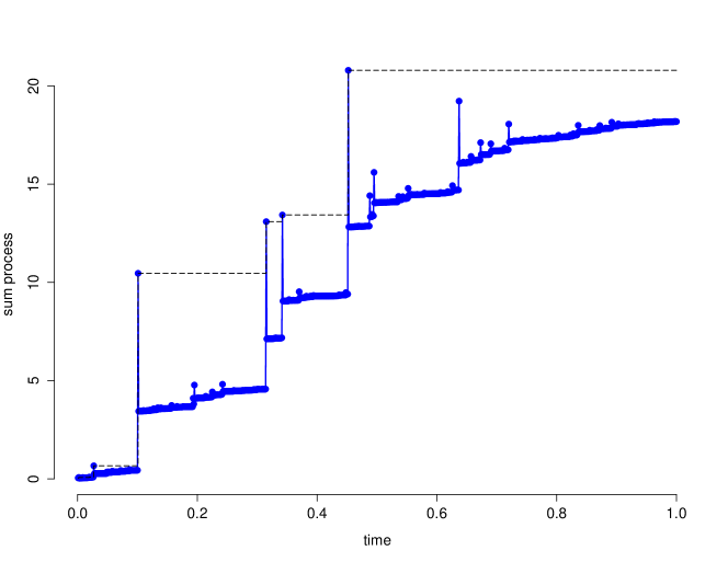
Figure 1: A simulated sample path of the process $S_{n}$ in the case of linear sequence $X_{t}=\xi_{t}-0.7\xi_{t-1}$ with index of regular variation $\alpha=0.7$ in blue. Observe that due to downward “corrections” after each large jump, in the limit the paths of the process $S_{n}$ cannot converge to a càdlàg function.

Remark 4.10.

We do not exclude the case $\sum_{j\in\mathbb{Z}}Q_{j}=0$ with probability one, as happens for instance in Example 4.9 with $c=-1$. In such a case, the càdlàg component $V$ is simply the null process.

Example 4.11.

Consider a stationary GARCH$(1,1)$ process

$$X_{t}=\sigma_{t}Z_{t},\;\;\sigma_{t}^{2}=\alpha_{0}+\alpha_{1}X_{t-1}^{2}+\beta_{1}\sigma_{t-1}^{2},\;\;t\in\mathbb{Z},$$

where $\alpha_{0},\alpha_{1},\beta_{1}>0,$ and $\{Z_{t},t\in\mathbb{Z}\}$ is a sequence of i.i.d. random variables with mean zero and variance one. Under mild conditions the process $\{X_{t}\}$ is regularly varying and satisfies Assumptions 1.1 and 3.5. These hold for instance in the case of standard normal innovations ${Z}_{t}$ and sufficiently small parameters $\alpha_{1},\beta_{1}$, see (Mikosch and Wintenberger,, 2013, Section 4.4). Consider for simplicity such a stationary GARCH$(1,1)$ process with tail index $\alpha\in(0,1).$ Since all the conditions of Theorem 4.5 are met, its partial sum process has a limit in the space $E$ (cf. Figure 2).

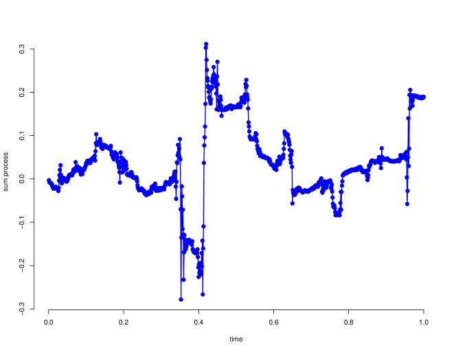
Figure 2: A simulated sample path of the process $S_{n}$ in the case of GARCH$(1,1)$ process with parameters $\alpha_{0}=0.01,\,\alpha_{1}=1.45$ and $\beta_{1}=0.1,$ and tail index $\alpha$ between $0.5$ and 1.

Proof of Theorem 4.5.

The proof is split into the cases $\alpha<1$ which is simpler, and the case $\alpha\in[1,2)$ where centering and truncation introduce additional technical difficulties.

1. Assume first that $\alpha\in(0,1).$ We divide the proof into several steps.

   1. For every $\epsilon>0$, consider the functions $s^{\epsilon},u^{\epsilon}$ and $v^{\epsilon}$ defined on $\tilde{l}_{0}$ by

      $$s^{\epsilon}(\tilde{\boldsymbol{x}})=\sum_{j}x_{j}\mathbbm{1}_{\{|x_{j}|>\epsilon\}}\;,\ \ u^{\epsilon}(\tilde{\boldsymbol{x}})=\inf_{k}\sum_{j\leq k}x_{j}\mathbbm{1}_{\{|x_{j}|>\epsilon\}}\;,\ \ v^{\epsilon}(\tilde{\boldsymbol{x}})=\sup_{k}\sum_{j\leq k}x_{j}\mathbbm{1}_{\{|x_{j}|>\epsilon\}}\;,$$

      and define the mapping $T^{\epsilon}:\mathcal{M}_{p}([0,1]\times\tilde{l}_{0}\setminus\{\tilde{\boldsymbol{0}}\})\rightarrow E$ by setting, for $\gamma=\sum_{i=1}^{\infty}\delta_{t_{i},\tilde{\boldsymbol{x}}^{i}},$

      $$T^{\epsilon}\gamma=\left(\left(\sum_{t_{i}\leq t}s^{\epsilon}(\tilde{\boldsymbol{x}}^{i})\right)_{t\in[0,1]}\;,\{t_{i}:\|\tilde{\boldsymbol{x}}^{i}\|_{\infty}>\epsilon\},\{I(t_{i}):\|\tilde{\boldsymbol{x}}^{i}\|_{\infty}>\epsilon\}\right),$$

      where

      $$I(t_{i})=\sum_{t_{j}<t_{i}}s^{\epsilon}(\tilde{\boldsymbol{x}}^{j})+\left[\sum_{t_{k}=t_{i}}u^{\epsilon}(\tilde{\boldsymbol{x}}^{k}),\sum_{t_{k}=t_{i}}v^{\epsilon}(\tilde{\boldsymbol{x}}^{k})\right].$$

      Since $m$ belongs $\mathcal{M}_{p}([0,1]\times\tilde{l}_{0}\setminus\{\tilde{\boldsymbol{0}}\}),$ there is only a finite number of points $(t_{i},\tilde{\boldsymbol{x}}^{i})$ such that $\|\tilde{\boldsymbol{x}}^{i}\|_{\infty}>\epsilon$ and furthermore, every $\tilde{\boldsymbol{x}}^{i}$ has at most finitely many coordinates greater than $\epsilon.$ Therefore, the mapping $T^{\epsilon}$ is well-defined, that is, $T^{\epsilon}\gamma$ is a proper element of $E.$

      Next, we define the subsets of $\mathcal{M}_{p}([0,1]\times\tilde{l}_{0}\setminus\{\tilde{\boldsymbol{0}}\})$ by

      $$\Lambda_{1} =\left\{\sum_{i=1}^{\infty}\delta_{t_{i},\tilde{\boldsymbol{x}}^{i}}:|x_{j}^{i}|\neq\epsilon,i\geq 1,j\in\mathbb{Z}\right\}\;,$$

      $$\Lambda_{2} =\{\sum_{i=1}^{\infty}\delta_{t_{i},\tilde{\boldsymbol{x}}^{i}}:0<t_{i}<1\textnormal{ and }t_{i}\neq t_{j}\textnormal{ for every }i>j\geq 1\}.$$

      We claim that $T^{\epsilon}$ is continuous on the set $\Lambda_{1}\cap\Lambda_{2}.$ Assume that $\gamma_{n}\rightarrow_{w^{\#}}\gamma=\sum_{i=1}^{\infty}\delta_{t_{i},\tilde{\boldsymbol{x}}^{i}}\in\Lambda_{1}\cap\Lambda_{2}$. By an adaptation of (Resnick,, 1987, Proposition 3.13), this convergence implies that the finitely many points of $\gamma_{n}$ in every set $B$ bounded for $\tilde{d}^{\prime}$ and such that $\gamma(\partial B)=0$ converge pointwise to the finitely many points of $\gamma$ in $B$. In particular, this holds for $B=\{(t,\tilde{\boldsymbol{x}})\,:\,\|\tilde{\boldsymbol{x}}\|_{\infty}>\epsilon\}$ and it follows that for all $t_{1}<t_{2}$ in $[0,1]$ such that $\gamma(\{t_{1},t_{2}\}\times\tilde{l}_{0}\setminus\{\tilde{\boldsymbol{0}}\})=0$,

      $$M_{t_{1},t_{2}}(T^{\epsilon}(\gamma_{n}))\rightarrow M_{t_{1},t_{2}}(T^{\epsilon}(\gamma))\text{ in }\mathbb{R}$$

      and

      $$M_{t_{1},t_{2}}(-T^{\epsilon}(\gamma_{n}))\rightarrow M_{t_{1},t_{2}}(-T^{\epsilon}(\gamma))\text{ in }\mathbb{R},$$

      whith the local-maximum function $M_{t_{1},t_{2}}$ defined as in (4.6). Since the set of all such times is dense in $[0,1]$ and includes $0$ and $1$, an application of Theorem 4.3 gives that

      $$T^{\epsilon}(\gamma_{n})\rightarrow T^{\epsilon}(\gamma)$$

      in $E$ endowed with the $M_{2}$ topology.

      Recall the point process $N^{\prime\prime}=\sum_{i=1}^{\infty}\delta_{(T_{i},P_{i}\boldsymbol{Q}_{i})}$ from (4.8). Since the mean measure of $\sum_{i=1}^{\infty}\delta_{(T_{i},P_{i})}$ does not have atoms, it is clear that $N^{\prime\prime}\in\Lambda_{1}\cap\Lambda_{2}$ a.s. Therefore, by the convergence $N^{\prime\prime}_{n}\stackrel{{\scriptstyle d}}{{\longrightarrow}}N^{\prime\prime}$ and the continuous mapping argument

      $$\tilde{S}_{n,\epsilon}^{\prime}\stackrel{{\scriptstyle d}}{{\longrightarrow}}S_{\epsilon}^{\prime}\;,$$

      where $\tilde{S}_{n,\epsilon}^{\prime}=T^{\epsilon}(N_{n}^{\prime\prime})$ and $S_{\epsilon}^{\prime}=T^{\epsilon}(N^{\prime\prime}).$

   2. Recall that $W_{i}=\sum_{j\in\mathbb{Z}}|Q_{i,j}|$ and $\sum_{i=1}^{\infty}\delta_{P_{i}W_{i}}$ is a Poisson point process on $(0,\infty]$ with intensity measure $\theta\mathbb{E}[W_{i}^{\alpha}]\alpha y^{-\alpha-1}dy$ (see Remark 4.6). Since $\alpha<1$, one can sum up the points $\{P_{i}W_{i}\},$ i.e.

      $$\sum_{i=1}^{\infty}P_{i}W_{i}=\sum_{i=1}^{\infty}\sum_{j\in\mathbb{Z}}P_{i}|Q_{i,j}|<\infty\;\text{ a.s.}$$ (4.16)

      Therefore, defining $s(\tilde{\boldsymbol{x}})=\sum_{j}x_{j}$, we obtain that the process

      $$V(t)=\sum_{T_{i}\leq t}s(P_{i}\boldsymbol{Q}_{i})\;,\;t\in[0,1]\;,$$

      is almost surely a well-defined element in $D$ and moreover, it is an $\alpha$-stable Lévy process. Further, we define an element $V^{\prime}$ in $E([0,1],\mathbb{R})$ by

      $$V^{\prime}=\left(V,\{T_{i}\}_{i\in\mathbb{N}},\{I(T_{i})\}_{i\in\mathbb{N}}\right)\;,$$ (4.17)

      where

      $$I(T_{i}) =V(T_{i}-)+\left[u(P_{i}\boldsymbol{Q}_{i}),v(P_{i}\boldsymbol{Q}_{i})\right]\;,$$

      $$u(\tilde{\boldsymbol{x}}) =\inf_{k}\sum_{j\leq k}x_{j}\;,\ \ v(\tilde{\boldsymbol{x}})=\sup_{k}\sum_{j\leq k}x_{j}\;.$$

      Since for every $\delta>0$ there are at most finitely many points $P_{i}W_{i}$ such that $P_{i}W_{i}>\delta$ and $diam(I(T_{i}))=v(P_{i}\boldsymbol{Q}_{i})-u(P_{i}\boldsymbol{Q}_{i})\leq P_{i}W_{i},$ $V^{\prime}$ is indeed a proper element of $E$ a.s.

      We now show that, as $\epsilon\rightarrow 0,$ the limits $S_{\epsilon}^{\prime}$ from the previous step converge to $V^{\prime}$ in $(E,m)$ almost surely. Recall the uniform metric $m^{*}$ on $E$ defined in (4.2). By (4.16) and dominated convergence theorem

      $$m^{*}(S_{\epsilon}^{\prime},V^{\prime})=\sup_{0\leq t\leq 1}m(S_{\epsilon}^{\prime}(t),V^{\prime}(t))\leq\sum_{i=1}^{\infty}\sum_{j\in\mathbb{Z}}P_{i}|Q_{ij}|\mathbbm{1}_{\{P_{i}|Q_{ij}|\leq\epsilon\}}\rightarrow 0\;,$$ (4.18)

      almost surely as $\epsilon\rightarrow 0$. Indeed, let $S_{\epsilon}$ be the càdlàg part of $S_{\epsilon}^{\prime},$ i.e.

      $$S_{\epsilon}(t)=\sum_{T_{i}\leq t}s^{\epsilon}(P_{i}\boldsymbol{Q}_{i})=\sum_{T_{i}\leq t}\sum_{j\in\mathbb{Z}}P_{i}Q_{i,j}\mathbbm{1}_{\{|P_{i}Q_{i,j}|>\epsilon\}}\;,\;t\in[0,1]\;.$$

      If $t\notin\{T_{i}\}$ then

      $$m(S_{\epsilon}^{\prime}(t),V^{\prime}(t))=|S_{\epsilon}(t)-V(t)|\leq\sum_{T_{i}\leq t}\sum_{j\in\mathbb{Z}}P_{i}|Q_{i,j}|\mathbbm{1}_{\{P_{i}|Q_{ij}|\leq\epsilon\}}.$$

      Further, when $t=T_{k}$ for some $k\in\mathbb{Z},$ by using (4.4) we obtain

      $$m(S_{\epsilon}^{\prime}(t),V^{\prime}(t)) \leq|(S_{\epsilon}(T_{k}-)+v^{\epsilon}(P_{k}\boldsymbol{Q}_{k}))-(V(T_{k}-)+v(P_{k}\boldsymbol{Q}_{k}))|$$ (4.19)

      $$\vee|(S_{\epsilon}(T_{k}-)+u^{\epsilon}(P_{k}\boldsymbol{Q}_{k}))-(V(T_{k}-)+u(P_{k}\boldsymbol{Q}_{k}))|.$$

      The first term on the right-hand side of the equation above is bounded by

      $$\left|\sum_{T_{i}<T_{k}}\sum_{j\in\mathbb{Z}}P_{i}Q_{i,j}\mathbbm{1}_{\{P_{i}|Q_{ij}|\leq\epsilon\}}\right|+\left|\sup_{l\in\mathbb{Z}}\sum_{j\leq l}P_{k}Q_{k,j}\mathbbm{1}_{\{P_{i}|Q_{i,j}|>\epsilon\}}-\sup_{l\in\mathbb{Z}}\sum_{j\leq l}P_{k}Q_{k,j}\right|$$

      $$\leq\left|\sum_{T_{i}<T_{k}}\sum_{j\in\mathbb{Z}}P_{i}Q_{i,j}\mathbbm{1}_{\{P_{i}|Q_{ij}|\leq\epsilon\}}\right|+\sup_{l\in\mathbb{Z}}\left|\sum_{j\leq l}P_{k}Q_{k,j}\mathbbm{1}_{\{P_{i}|Q_{k,j}|>\epsilon\}}-\sum_{j\leq l}P_{k}Q_{k,j}\right|$$

      $$\leq\sum_{T_{i}\leq T_{k}}\sum_{j\in\mathbb{Z}}P_{i}|Q_{i,j}|\mathbbm{1}_{\{P_{i}|Q_{i,j}|\leq\epsilon\}}.$$

      Since, by similar arguments, one can obtain the same bound for the second term on the right-hand side of (4.19), (4.18) holds. It now follows from (4.3) that

      $$S_{\epsilon}^{\prime}\rightarrow V^{\prime}$$

      almost surely in $(E,m).$

   3. Recall that

      $$\boldsymbol{X}_{n,i}=(X_{(i-1)r_{n}+1},\dots,X_{ir_{n}})/a_{n}$$

      for $i=1,\dots,k_{n}$ and let $\tilde{S}_{n}^{\prime}$ be an element in $E$ defined by

      $$\left(\left(\sum_{i/k_{n}\leq t}s(\boldsymbol{X}_{n,i})\right)_{t\in[0,1]}\;,\{i/k_{n}\}_{i=1}^{k_{n}},\{I(i/k_{n})\}_{i=1}^{k_{n}}\right)\;,$$

      where

      $$I(i/k_{n})=\sum_{j<i}s(\boldsymbol{X}_{n,j})+\left[u(\boldsymbol{X}_{n,i}),v(\boldsymbol{X}_{n,i})\right]\;.$$

      By (Billingsley,, 1968, Theorem 4.2) and the previous two steps, to show that

      $$\tilde{S}_{n}^{\prime}\stackrel{{\scriptstyle d}}{{\longrightarrow}}V^{\prime}$$

      in $(E,m_{E})$, it suffices to prove that, for all $\delta>0,$

      $$\lim_{\epsilon\rightarrow 0}\limsup_{n\rightarrow\infty}\mathbb{P}(m_{E}(\tilde{S}_{n,\epsilon}^{\prime},\tilde{S}_{n}^{\prime})>\delta)=0\;.$$ (4.20)

      Note first that, by the same arguments as in the previous step, we have

      $$m^{*}(\tilde{S}_{n,\epsilon}^{\prime},\tilde{S}_{n}^{\prime})\leq\sum_{j=1}^{k_{n}r_{n}}\frac{|X_{j}|}{a_{n}}\mathbbm{1}_{\{|X_{j}|\leq a_{n}\epsilon\}}\;.$$

      By (4.3), Markov’s inequality and Karamata’s theorem ((Bingham et al.,, 1989, Proposition 1.5.8))

      $$\limsup_{n\to\infty}\mathbb{P}(m_{E}(\tilde{S}_{n,\epsilon}^{\prime},\tilde{S}_{n}^{\prime})>\delta) \leq\limsup_{n\to\infty}\frac{k_{n}r_{n}}{\delta a_{n}}\mathbb{E}\left[|X_{1}|\mathbbm{1}_{\{|X_{1}|\leq a_{n}\epsilon\}}\right]$$

      $$=\lim_{n\to\infty}\frac{n}{\delta a_{n}}\cdot\frac{\alpha a_{n}\epsilon\mathbb{P}(|X_{1}|>a_{n}\epsilon)}{1-\alpha}=\frac{\alpha}{(1-\alpha)\delta}\epsilon^{1-\alpha}\;.$$

      This proves (4.20) since $\alpha<1$ and hence

      $$\tilde{S}_{n}^{\prime}\stackrel{{\scriptstyle d}}{{\longrightarrow}}V^{\prime}$$

      in $(E,m_{E})$.

   4. Finally, to show that the original partial sum process $S_{n}$ (and therefore $V_{n}$ since $\alpha\in(0,1)$) also converges in distribution to $V^{\prime}$ in $(E,m_{E})$, by Slutsky argument it suffices to prove that

      $$m_{E}(S_{n},\tilde{S}_{n}^{\prime})\stackrel{{\scriptstyle P}}{{\longrightarrow}}0\;.$$ (4.21)

      Recall that $k_{n}=\lfloor n/r_{n}\rfloor$ so $\frac{ir_{n}}{n}\leq\frac{i}{k_{n}}$ for all $i=0,1,\dots,k_{n}$ and moreover

      $$\frac{i}{k_{n}}-\frac{ir_{n}}{n}=\frac{i}{k_{n}}\left(1-\frac{k_{n}r_{n}}{n}\right)\leq 1-\frac{\lfloor n/r_{n}\rfloor}{n/r_{n}}=1-\left(1-\frac{\{n/r_{n}\}}{n/r_{n}}\right)\leq\frac{r_{n}}{n}\;.$$ (4.22)

      Let $d_{n,i}$ for $i=0,\dots,k_{n}-1$ be the Hausdorff distance between restrictions of graphs $\Gamma_{S_{n}}$ and $\Gamma_{\tilde{S}_{n}^{\prime}}$ on time intervals $(\frac{ir_{n}}{n},\frac{(i+1)r_{n}}{n}]$ and $(\frac{i}{k_{n}},\frac{i+1}{k_{n}}],$ respectively (see Figure 3).

      

      

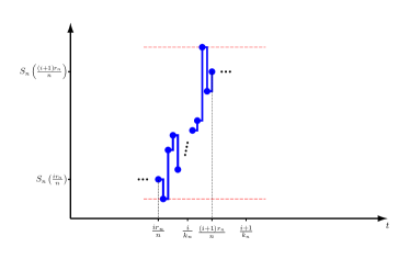
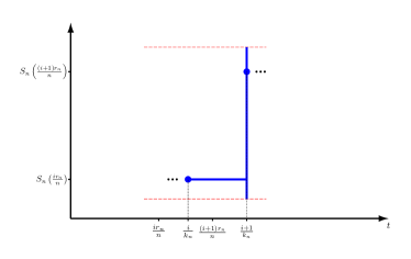
      Figure 3: Restrictions of graphs $\Gamma_{S_{n}}$ and $\Gamma_{\tilde{S}_{n}^{\prime}}$ on time intervals $(\frac{ir_{n}}{n},\frac{(i+1)r_{n}}{n}]$ and $(\frac{i}{k_{n}},\frac{i+1}{k_{n}}],$ respectively.

      First note that, by (4.22), the time distance between any two points on these graphs is at most $2r_{n}/n.$ Further, by construction, $S_{n}$ and $\tilde{S}_{n}^{\prime}$ have the same range of values on these time intervals. More precisely,

      $$\bigcup_{t\in(\frac{ir_{n}}{n},\frac{(i+1)r_{n}}{n}]}\{z\in\mathbb{R}\;:\;(t,z)\in\Gamma_{S_{n}}\}=\bigcup_{t\in(\frac{i}{k_{n}},\frac{i+1}{k_{n}}]}\{z\in\mathbb{R}\;:\;(t,z)\in\Gamma_{\tilde{S}_{n}^{\prime}}\}=\tilde{S}_{n}^{\prime}((i+1)/k_{n})\;.$$

      Therefore, the distance between the graphs comes only from the time component, i.e.

      $$d_{n,i}\leq\frac{2r_{n}}{n}\rightarrow 0\;,\;\text{ as }n\rightarrow\infty\;,$$

      for all $i=0,1,\dots,k_{n}-1.$

      Moreover, if we let $d_{n,k_{n}}$ be the Hausdorff distance between the restriction of the graph $\Gamma_{S_{n}}$ on $(\frac{k_{n}r_{n}}{n},1]$ and the interval $(1,\tilde{S}_{n}^{\prime}(1)),$ it holds that

      $$d_{n,k_{n}}\leq\frac{r_{n}}{n}\vee\sum_{j=k_{n}r_{n}+1}^{n}\frac{|X_{j}|}{a_{n}}\stackrel{{\scriptstyle P}}{{\longrightarrow}}0,$$

      as $n\rightarrow\infty.$ Hence, (4.21) holds since

      $$m_{E}(S_{n},\tilde{S}_{n}^{\prime})\leq\bigvee_{i=0}^{k_{n}}d_{n,i},$$

      and this finishes the proof in the case $\alpha\in(0,1)$.

2. Assume now that $\alpha\in[1,2)$. As shown in a1 in the proof of a, it holds that

   $$\tilde{S}_{n,\epsilon}^{\prime}\stackrel{{\scriptstyle d}}{{\longrightarrow}}S_{\epsilon}^{\prime}$$ (4.23)

   in $E,$ where $\tilde{S}_{n,\epsilon}^{\prime}=T^{\epsilon}(N_{n}^{\prime\prime})$ and $S_{\epsilon}^{\prime}=T^{\epsilon}(N^{\prime\prime})$.

   For every $\epsilon>0$ define a càdlàg process $S_{n,\epsilon}$ by setting, for $t\in[0,1],$

   $$S_{n,\epsilon}(t)=\sum_{i=1}^{\lfloor nt\rfloor}\frac{X_{i}}{a_{n}}\mathbbm{1}_{\{|X_{i}|/a_{n}>\epsilon\}}.$$

   Using the same arguments as in a4 in the proof of a, it holds that, as $n\rightarrow\infty,$

   $$m_{E}(S_{n,\epsilon},\tilde{S}_{n,\epsilon}^{\prime})\stackrel{{\scriptstyle P}}{{\longrightarrow}}0\;.$$ (4.24)

   Therefore, by Slutsky argument it follows from (4.24) and (4.23) that

   $$S_{n,\epsilon}\stackrel{{\scriptstyle d}}{{\longrightarrow}}S_{\epsilon}^{\prime}$$ (4.25)

   in $(E,m_{E})$.

   Since $\alpha\in[1,2)$ we need to introduce centering, so we define the càdlàg process $V_{n,\epsilon}$ by setting, for $t\in[0,1],$

   $$V_{n,\epsilon}(t)=S_{n,\epsilon}(t)-\lfloor nt\rfloor\mathbb{E}\left(\frac{X_{1}}{a_{n}}\mathbbm{1}_{\{\epsilon<|X_{1}|/a_{n}\leq 1\}}\right)\;.$$

   From (1.4) we have, for any $t\in[0,1],$ as $n\rightarrow\infty,$

   $$\lfloor nt\rfloor\mathbb{E}\left(\frac{X_{1}}{a_{n}}\mathbbm{1}_{\{\epsilon<|X_{1}|/a_{n}\leq 1\}}\right)\rightarrow t\int_{\{x\;:\;\epsilon<|x|\leq 1\}}x\mu(dx).$$ (4.26)

   Since the limit function above is continuous and the convergence is uniform on $[0,1]$, by Lemma 6.3 and (4.25) it follows that

   $$V_{n,\epsilon}\stackrel{{\scriptstyle d}}{{\longrightarrow}}V_{\epsilon}^{\prime}$$ (4.27)

   in $E$, where $V_{\epsilon}^{\prime}$ is given by (see Remark 4.2)

   $$V_{\epsilon}^{\prime}(t) =S_{\epsilon}^{\prime}(t)-t\int_{\{x\;:\;\epsilon<|x|\leq 1\}}x\mu(dx)\;.$$

   Let $V_{\epsilon}$ be the càdlàg part of $V_{\epsilon}^{\prime},$ i.e.,

   $$V_{\epsilon}(t) =\sum_{T_{i}\leq t}s^{\epsilon}(P_{i}\boldsymbol{Q}_{i})-t\int_{\{x\;:\;\epsilon<|x|\leq 1\}}x\mu(dx)\;.$$ (4.28)

   By Lemma 6.4, there exist an $\alpha$-stable Lévy process $V$ such that $V_{\epsilon}$ converges uniformly almost surely (along some subsequence) to $V$. Next, as in a2 in the proof of a we can define a element $V^{\prime}$ in $E$ by

   $$V^{\prime}=\left(V,\{T_{i}\}_{i\in\mathbb{N}},\{I(T_{i})\}_{i\in\mathbb{N}}\right)\;,$$ (4.29)

   where

   $$I(T_{i})=V(T_{i}-)+\left[u(P_{i}\boldsymbol{Q}_{i}),v(P_{i}\boldsymbol{Q}_{i})\right]\;,$$ (4.30)

   Also, one can argue similarly to the proof of (4.18) to conclude that

   $$m^{*}(V^{\prime},V_{\epsilon}^{\prime})\leq||V-V_{\epsilon}||_{\infty}+\sup_{i\in\mathbb{N}}\sum_{j\in\mathbb{Z}}P_{i}|Q_{i,j}|\mathbbm{1}_{\{P_{i}|Q_{i,j}|\leq\epsilon\}}\;.$$

   Now it follows from (4.3), (4.12) and a.s. uniform convergence of $V_{\epsilon}$ to $V$ that

   $$V_{\epsilon}^{\prime}\rightarrow V^{\prime}\;\text{a.s.}$$ (4.31)

   in $(E,m_{E})$.

   Finally, by (4.27), (4.31) and (Billingsley,, 1968, Theorem 4.2), to show that

   $$V_{n}\stackrel{{\scriptstyle d}}{{\longrightarrow}}V^{\prime},$$ (4.32)

   in $(E,m_{E})$, it suffices to prove that, for all $\delta>0,$

   $$\lim_{\epsilon\rightarrow 0}\limsup_{n\rightarrow\infty}\mathbb{P}(m_{E}(V_{n,\epsilon},V_{n})>\delta)=0\;.$$ (4.33)

   But this follows from Assumption 4.4 and (4.3) since

   $$m^{*}(V_{n,\epsilon},V_{n})\leq\max_{1\leq k\leq n}\left|\sum_{i=1}^{k}\left(\frac{X_{i}}{a_{n}}\mathbbm{1}_{\{|X_{i}|/a_{n}\leq\epsilon\}}-\mathbb{E}\left[\frac{X_{i}}{a_{n}}\mathbbm{1}_{\{|X_{i}|/a_{n}\leq\epsilon\}}\right]\right)\right|.$$

   Hence (4.32) holds and this finishes the proof.

∎

4.3 Supremum of the partial sum process

We next show that the supremum of the partial sum process converges in distribution in $D$ endowed with the $M_{1}$ topology, where the limit is the “running supremum” of the limit process $V^{\prime}$ from Theorem 4.5.

Let $V$ be the Lévy process defined in (4.11) and define the process $V^{+}$ on $[0,1]$ by

$$V^{+}(t)= \begin{cases}V(t)\;,&t\notin\{T_{j}\}_{j\in\mathbb{N}}\\ V(t-)+\sup_{k\in\mathbb{Z}}\sum_{j\leq k}P_{i}Q_{i,j}\;,&t=T_{i}\text{ for some }i\in\mathbb{N}.\end{cases}$$

Define $V^{-}$ analogously using infimum instead of supremum. Note that $V^{+}$ and $V^{-}$ need not be right-continuous at the jump times $T_{j}.$ However, their partial supremum or infimum are càdlàg functions.

Theorem 4.12.

Under the same conditions as in Theorem 4.5, it holds that

$$\left(\sup_{s\leq t}V_{n}(s)\right)_{t\in[0,1]}\stackrel{{\scriptstyle d}}{{\longrightarrow}}\left(\sup_{s\leq t}V^{+}(s)\right)_{t\in[0,1]}\;,$$

and

$$\left(\inf_{s\leq t}V_{n}(s)\right)_{t\in[0,1]}\stackrel{{\scriptstyle d}}{{\longrightarrow}}\left(\inf_{s\leq t}V^{-}(s)\right)_{t\in[0,1]}\;,$$

jointly in $D([0,1],\mathbb{R})$ endowed with the $M_{1}$ topology.

Proof.

We prove the result only for the supremum of the partial sum process since the infimum case is completely analogous and joint convergence holds since we are applying the continuous mapping argument to the same process.

Define the mapping $\;\sup:E([0,1],\mathbb{R})\rightarrow D([0,1],\mathbb{R})$ by

$$\sup(x^{\prime})(t)=\sup\{z:z\in x^{\prime}(s),0\leq s\leq t\}\;.$$

Note that $\sup(x^{\prime})$ is non-decreasing and since for every $\delta>0$ there are at most finitely many times $t$ for which the $diam(x^{\prime}(t))$ is greater than $\delta$, by (Whitt,, 2002, Theorem 15.4.1.) it follows easily that this mapping is well-defined, i.e. that $\sup(x^{\prime})$ is indeed an element in $D.$ Also, by construction,

$$\sup(V^{\prime})=\left(\sup_{s\leq t}V^{+}(s)\right)_{t\in[0,1]}$$

and

$$\sup(V_{n})=\left(\sup_{s\leq t}V_{n}(s)\right)_{t\in[0,1]}.$$

Define the subset of $E$ by

$$\Lambda=\left\{x^{\prime}\in E\>:\>x^{\prime}(0)=\{0\}\right\}$$

and assume that $x_{n}^{\prime}\rightarrow x^{\prime}$ in $(E,m_{E}),$ where $x_{n}^{\prime},x^{\prime}\in\Lambda$. By Theorem 4.3 it follows that

$$\sup(x_{n}^{\prime})(t)=M_{0,t}(x_{n}^{\prime})\rightarrow M_{0,t}(x^{\prime})=\sup(x^{\prime})(t)$$

for all $t$ in a dense subset of (0,1], including $1$. Also, the convergence trivially holds for $t=0$ since $\sup(x_{n}^{\prime})(0)=\sup(x^{\prime})(0)=0$ for all $n\in\mathbb{N}.$ Since $\sup(x^{\prime})$ is non-decreasing for all $x^{\prime}\in E,$ we can apply (Whitt,, 2002, Corollary 12.5.1) and conclude that

$$\sup(x_{n}^{\prime})\rightarrow\sup(x^{\prime})$$

in $D$ endowed with $M_{1}$ topology. Since $V_{n},V^{\prime}\in\Lambda$ almost surely, by Theorem 4.5 and continuous mapping argument it follows that

$$\left(\sup_{s\leq t}V_{n}(s)\right)_{t\in[0,1]}\stackrel{{\scriptstyle d}}{{\longrightarrow}}\left(\sup_{s\leq t}V^{+}(s)\right)_{t\in[0,1]}$$

in $D$ endowed with $M_{1}$ topology. ∎

Remark 4.13.

Note that when $\sum_{j\in\mathbb{Z}}Q_{j}=0$ a.s., the limit for the supremum of the partial sum process in Theorem 4.12 is simply a so called Fréchet extremal process. For an illustration of the general limiting behavior of running maxima in the case of a linear processes, consider again the moving average of order 1 from Example 4.9. Figure 1 shows a path (dashed line) of the running maxima of the MA$(1)$ process $X_{t}=\xi_{t}-0.7\xi_{t-1}$.

4.4 $M_{2}$ convergence of the partial sum process

We can now characterize the convergence of the partial sum process in the $M_{2}$ topology in $D([0,1])$ by an appropriate condition on the tail process of the sequence $\{X_{t},t\in\mathbb{Z}\}$.

Assumption 4.14.

The sequence $\{Q_{j},j\in\mathbb{Z}\}$ satisfies

$$-\left(\sum_{j\in\mathbb{Z}}Q_{j}\right)_{-}=\inf_{k\in\mathbb{Z}}\sum_{j\leq k}Q_{j}\leq\sup_{k\in\mathbb{Z}}\sum_{j\leq k}Q_{j}=\left(\sum_{j\in\mathbb{Z}}Q_{j}\right)_{+}\;\mbox{ a.s. }$$ (4.34)

i.e. $-s(\boldsymbol{Q})_{-}=u(\boldsymbol{Q})\leq v(\boldsymbol{Q})=s(\boldsymbol{Q})_{+}$ a.s.

Note that this assumption ensures that $\sum_{j\in\mathbb{Z}}Q_{j}\neq 0$ and that the limit process $V^{\prime}$ from Theorem 4.5 has sample paths in the subset $D^{\prime}$ of $E$ which was defined in (4.5). By Lemma 4.1, Theorem 4.5 and the continuous mapping theorem, the next result follows immediately.

Theorem 4.15.

If, in addition to conditions in Theorem 4.5, Assumption 4.14 holds, then

$$V_{n}\stackrel{{\scriptstyle d}}{{\longrightarrow}}V$$

in $D([0,1],\mathbb{R})$ endowed with the $M_{2}$ topology.

Since the supremum functional is continuous with respect to the $M_{2}$ topology, this result implies that the limit of the running supremum of the partial sum process is the running supremum of the limiting $\alpha$-stable Lévy process as in the case of i.i.d. random variables.

Example 4.16.

For the linear process $X_{t}=\sum_{j\in\mathbb{Z}}c_{j}\xi_{t-j}$ from Section 3.3 and Example 4.9, the corresponding sequence $\{Q_{j}\}$ was given in (3.8). It follows that the Condition (4.34) can be expressed as

$$-\left(\sum_{j\in\mathbb{Z}}c_{j}\right)_{-}=\inf_{k\in\mathbb{Z}}\sum_{j\leq k}c_{j}\leq\sup_{k\in\mathbb{Z}}\sum_{j\leq k}c_{j}=\left(\sum_{j\in\mathbb{Z}}c_{j}\right)_{+}\;.$$ (4.35)

This is exactly (Basrak and Krizmanić,, 2014, Condition 3.2). Note that (4.35) implies that

$$\left|\sum_{j\in\mathbb{Z}}c_{j}\right|>0\;.$$

5 Record times

In this section we study record times in a stationary sequence $\{X_{t},t\in\mathbb{Z}\}$. Since record times remain unaltered after a strictly increasing transformation, the main result below holds for stationary sequences with a general marginal distribution as long as they can be monotonically transformed into a regularly varying sequence.

We start by introducing the notion of records for sequences in $\tilde{l}_{0}$. For $y\geq 0$ and $\boldsymbol{x}=\{x_{j}\}\in\tilde{l}_{0}$ define

$$R^{\boldsymbol{x}}(y)=\sum_{j=-\infty}^{\infty}\mathbbm{1}_{\{x_{j}>y\vee\sup_{i<j}x_{i}\}}\,,$$

representing the number of records in the sequence $\boldsymbol{x}$ larger than $y$, which is finite for $\boldsymbol{x}\in\tilde{l}_{0}$. For notational simplicity, we suppress notation $\tilde{\boldsymbol{x}}$ in this section.

Let $\gamma=\sum_{i=1}^{\infty}\delta_{t_{i},\boldsymbol{x}^{i}}\in\mathcal{M}_{p}({[0,\infty)\times\tilde{l}_{0}\setminus\{\tilde{\boldsymbol{0}}\}})$, where $\boldsymbol{x}^{i}=\{x^{i}_{j}\}\in\tilde{l}_{0}$. Define, for $t>0$

$$M^{\gamma}(t)=\sup_{t_{i}\leq t}\|\boldsymbol{x}^{i}\|_{\infty}\;,\quad M^{\gamma}(t-)=\sup_{t_{i}<t}\|\boldsymbol{x}^{i}\|_{\infty}\;,$$

where we set $\sup\emptyset=0$ for convenience. Next, let $R_{\gamma}$ be the (counting) point process on $(0,\infty)$ defined by

$$R_{\gamma} =\sum_{i}\delta_{t_{i}}R^{\boldsymbol{x}^{i}}(M^{\gamma}(t_{i}-))\;,$$

hence for arbitrary $0<a<b$

$$R_{\gamma}(a,b] =\sum_{a<t_{i}\leq b}\sum_{j=-\infty}^{\infty}\mathbbm{1}_{\{x^{i}_{j}>M^{\gamma}(t_{i}-)\vee\sup_{k<j}x^{i}_{k}\}}\;.$$

Consider the following subset of $\mathcal{M}_{p}({[0,\infty)\times\tilde{l}_{0}\setminus\{\tilde{\boldsymbol{0}}\}})$

$$A= \{\gamma=\sum_{i=1}^{\infty}\delta_{t_{i},\boldsymbol{x}^{i}}:\mbox{ such that }M^{\gamma}(t)>0\mbox{ for all $t>0$, while }$$

$$\mbox{all $t_{i}$'s are mutually different as well as all nonzero $x^{i}_{j}$'s}\}\,.$$

The space $\mathcal{M}_{p}((0,\infty))$ is endowed with the $w^{\#}$ topology which is equivalent to the usual vague topology since $(0,\infty)$ is locally compact and separable.

Lemma 5.1.

The mapping $\gamma\mapsto R_{\gamma}$ from $\mathcal{M}_{p}({[0,\infty)\times\tilde{l}_{0}\setminus\{\tilde{\boldsymbol{0}}\}})$ to $\mathcal{M}_{p}((0,\infty))$ is continuous at every $\gamma\in A$.

Proof.

Fix an arbitrary $\gamma\in A$, and assume a sequence $\{\gamma_{n}\}$ in $\mathcal{M}_{p}([0,\infty)\times\tilde{l}_{0}\setminus\{\tilde{\boldsymbol{0}}\})$ satisfies $\gamma_{n}\rightarrow_{w^{\#}}\gamma$. We must prove that $R_{\gamma_{n}}$ converges vaguely to $R_{\gamma}$ in $\mathcal{M}_{p}((0,\infty))$. By the Portmanteau theorem, it is sufficient to show that that for all $0<a<b\in\{t_{i}\}^{c}$

$$R_{\gamma_{n}}(a,b]\to R_{\gamma}(a,b]\,,$$

as $n\to\infty$. For $0<a<b\in\{t_{i}\}^{c}$ there are finitely many time instances, say $t_{i_{1}},\ldots,t_{i_{k}}\in(a,b]$ such that $\|\boldsymbol{x}^{i_{l}}\|_{\infty}>M^{\gamma}(a)>0$, hence

$$R_{\gamma}(a,b] =\sum_{t_{i}\in(a,b]}R^{\boldsymbol{x}^{i}}(M^{\gamma}(t_{i}-))=\sum_{l=1}^{k}R^{\boldsymbol{x}^{i_{l}}}(M^{\gamma}(t_{i_{l}}-))\;.$$ (5.1)

For all $\gamma_{n}=\sum_{i=1}^{\infty}\delta_{t^{n}_{i},\boldsymbol{x}^{n,i}}$ with $n$ large enough, there also exist exactly $k$ (depending on $a$ and $b$) time instances $t^{n}_{i_{1}},\ldots,t^{n}_{i_{k}}\in(a,b]$ such that $\|\boldsymbol{x}^{n,i_{l}}\|_{\infty}>M^{\gamma}(a)$. Moreover, they satisfy $\boldsymbol{x}^{n,i_{l}}\to\boldsymbol{x}^{i_{l}}$ and $t^{n}_{i_{l}}\to t_{i_{l}}$ for $l=1,\ldots k$ as $n\to\infty$. Hence for $n$ large enough

$$R_{\gamma_{n}}(a,b] =\sum_{t^{n}_{i}\in(a,b]}R^{\boldsymbol{x}^{n,i}}(M^{\gamma_{n}}(t^{n}_{i}-))=\sum_{l=1}^{k}R^{\boldsymbol{x}^{n,i_{l}}}(M^{\gamma_{n}}(t^{n}_{i_{l}}-))\;.$$ (5.2)

Assume $y_{n}\to y>0$ and $\boldsymbol{x}^{n}\to\boldsymbol{x}=\{x_{j}\}$ where the non zero $x_{j}$ are pairwise distinct and $x_{j}\not=y$ for all $j\in\mathbb{Z}$. Then, it is straightforward to check that

$$R^{\boldsymbol{x}^{n}}(y_{n})\to R^{\boldsymbol{x}}(y)\,.$$

Observe further that for the choice of $t_{i_{l}}$, $t^{n}_{i_{l}}$ we made above, it holds that $M^{\gamma_{n}}(t^{n}_{i_{l}}-)\to M^{\gamma}(t_{i_{l}}-)$ since $t_{i}$’s are all different. Together with (5.1) and (5.2) this yields

$$R_{\gamma_{n}}(a,b]\to R_{\gamma}(a,b]$$

as $n\to\infty$. ∎

Since we are only interested in records, for convenience we consider a nonnegative stationary regularly varying sequence $\{X_{t},t\in\mathbb{Z}\}$.

Adopting the notation of Section 3.2, we denote

$$N^{\prime\prime}_{n}=\sum_{i=1}^{\infty}\delta_{(i/k_{n},\boldsymbol{X}_{n,j})}\;.$$ (5.3)

We will also need the point process $N_{n}$ defined by

$$N_{n}=\sum_{i=1}^{\infty}\delta_{(i/n,X_{i}/a_{n})}\;.$$

The process $N_{n}$ can be viewed as a point process on $[0,\infty)\times\mathbb{R}\setminus\{0\}$, but since $\mathbb{R}$ can be embedded in $\tilde{l}_{0}$ (by identifying a real number $x\neq 0$ to a sequence with exactly one nonzero coordinate equal to $x$), in the sequel we treat it as a process on the space $[0,\infty)\times\tilde{l}_{0}\setminus\{\tilde{\boldsymbol{0}}\}$.

As in the previous section, we will assume that

$$N^{\prime\prime}_{n}\stackrel{{\scriptstyle d}}{{\longrightarrow}}N^{\prime\prime}=\sum_{i=1}^{\infty}\delta_{(T_{i},P_{i}\boldsymbol{Q}_{i})}\;,$$ (5.4)

as $n\to\infty$, where $N^{\prime\prime}$ has the same form as in (4.8), but on the space $\mathcal{M}_{p}({[0,\infty)\times\tilde{l}_{0}\setminus\{\tilde{\boldsymbol{0}}\}})$. For $\beta$-mixing and linear processes, this convergence follows by direct extension of results in Section 3 from the state space $[0,1]\times\tilde{l}_{0}\setminus\{\tilde{\boldsymbol{0}}\}$ to $[0,T]\times\tilde{l}_{0}\setminus\{\tilde{\boldsymbol{0}}\}$ for arbitrary $T>0$.

Theorem 5.2.

Let $\{X_{t},t\in\mathbb{Z}\}$ be a stationary regularly varying sequence with tail index $\alpha>0$. Assume that the convergence in (5.4) holds and moreover that

$$\mathbb{P}(\mbox{all nonzero }Q_{1,j}\mbox{'s are mutually different})=1\;.$$

Then

$$R_{N_{n}}\stackrel{{\scriptstyle d}}{{\longrightarrow}}R_{N^{\prime\prime}}\,,$$

in $\mathcal{M}_{p}((0,\infty))$. Moreover, the limiting process is a compound Poisson process with representation

$$R_{N^{\prime\prime}}=\sum_{i\in\mathbb{Z}}\delta_{\tau_{i}}\kappa_{i}\,,$$

where $\sum_{i\in\mathbb{Z}}\delta_{\tau_{i}}$ is a Poisson point process on $(0,\infty)$ with intensity measure $x^{-1}\mathrm{d}x$ and $\{\kappa_{i}\}$ is a sequence of i.i.d. random variables independent of it with the same distribution as the integer valued random variable $R^{\boldsymbol{Q}_{1}}(1/\zeta)$ where $\zeta$ is a Pareto random variable with tail index $\alpha$, independent of $\boldsymbol{Q}_{1}$.

Proof.

Since they are constructed from the same sequence $X_{1},X_{2},\ldots$, the record values of the point process $N^{\prime\prime}_{n}$ in (5.3) correspond to the record values of the point process $N_{n}$. Using (5.4) and the additional assumption on the $Q$’s, by Lemma 5.1 it follows that

$$R_{N^{\prime\prime}_{n}}\stackrel{{\scriptstyle d}}{{\longrightarrow}}R_{N^{\prime\prime}}\,.$$ (5.5)

Note that record times $i/n$ of the process $N_{n}$ appear at slightly altered times $(\lfloor i/r_{n}\rfloor+1)/k_{n}$ in the process $N^{\prime\prime}_{n}$. However, asymptotically the record times are very close. Indeed, take $f\in C_{K}^{+}(0,\infty)$, then $f$ has a support on the set of the form $(a,b]$, $0<a<b$, which can be enlarged slightly to a set $(a-\epsilon,b+\epsilon]$, where $0<a-\epsilon$ for a sufficiently small $\epsilon>0$. Clearly, $f$ is continuous on that set, even uniformly. Note further that for any such $\epsilon$ there is an integer $n_{0}$ such that for $n\geq n_{0}$, $i/n\in(a,b]$ implies $(\lfloor i/r_{n}\rfloor+1)/k_{n}\in(a-\epsilon,b+\epsilon]$, and vice versa. Moreover, by uniform continuity of the function $f$, $n_{0}$ can be chosen such that for $n\geq n_{0}$,

$$\left|f\left(\frac{i}{n}\right)-f\left(\frac{\lfloor i/r_{n}\rfloor+1}{k_{n}}\right)\right|\leq\epsilon\;.$$

Consider now the difference between Laplace functionals of the point processes $R_{N^{\prime\prime}_{n}}$ and $R_{N_{n}}$ for a function $f\in C_{K}^{+}(0,\infty)$ as above. Since $\epsilon$ above can be made arbitrarily small, it follows that

$$\left|\mathbb{E}[\mathrm{e}^{-f(R_{N^{\prime\prime}_{n}})}]-\mathbb{E}[\mathrm{e}^{-f(R_{N_{n}})}]\right|\to 0\;,$$

which together with (5.5) yields the convergence statement of the theorem.

Consider now a point measure $\gamma=\sum_{i=1}^{\infty}\delta_{t_{i},\boldsymbol{x}^{i}}\in\mathcal{M}_{p}({[0,\infty)\times\tilde{l}_{0}\setminus\{\tilde{\boldsymbol{0}}\}})$, but such that all $\boldsymbol{x}^{i}$ have only nonnegative components and all $t_{i}$’s are mutually different. We say that a point measure $\gamma$ has a record at time $t$ if $(t,\boldsymbol{x})\in\{(t_{i},\boldsymbol{x}^{i}):i\geq 1\}$ and $M^{\gamma}(t-)=\sup_{t_{i}<t}\|\boldsymbol{x}^{i}\|_{\infty}<\|\boldsymbol{x}\|_{\infty}$ . Taking the order into account, at time $t$ we will see exactly $R^{\boldsymbol{x}}(M^{\gamma}(t-))$ records. Similarly, a point measure $\eta=\sum_{i=1}^{\infty}\delta_{t_{i},x_{i}}\in\mathcal{M}_{p}({[0,\infty)\times[0,\infty)})$ has a record at time $t$ with corresponding record value $x$, if $(t,x)\in\{(t_{i},x_{i}):i\geq 1\}$ and $\eta([0,t)\times[x,\infty))=0$.

To prove the representation of the limit, observe that $N^{\prime\prime}=\sum_{i=1}^{\infty}\delta_{(T_{i},P_{i}\boldsymbol{Q}_{i})}$ has records at exactly the same time instances as the process $M_{0}=\sum_{i=1}^{\infty}\delta_{(T_{i},P_{i})}$, since by the assumptions of the theorem and by definition of the sequences $\boldsymbol{Q}_{i}$, all of their components are in $[0,1]$ with one of them being exactly equal to 1. Because $M_{0}$ is a Poisson point process on $[0,\infty)\times(0,\infty]$ with intensity measure $\mathrm{d}x\times\mathrm{d}(-\theta y^{-\alpha})$, it has infinitely many points of in any set of the form $[a,b]\times[0,\epsilon]$ with $a<b$ and $\epsilon>0$. Hence, one can a.s. write the record times of $M_{0}$ as a double sided sequence $\tau_{n},\ n\in\mathbb{Z}$, such that $\tau_{n}<\tau_{n+1}$ for each $n$. Fix an arbitrary $s>0$, and assume without loss of generality that $\tau_{1}$ represents the first record time strictly greater than $s$, i.e. $\tau_{1}=\inf\{\tau_{i}:\tau_{i}>s\}$. Denote the corresponding successive record values by $U_{n}$; they clearly satisfy $U_{n}<U_{n+1}$ and $U_{n}=\sup_{T_{i}\leq\tau_{n}}P_{i}$ and $U_{0}=\sup_{T_{i}\leq s}P_{i}$. According to (Resnick,, 1987, Proposition 4.9), $\sum_{n\in\mathbb{Z}}\delta_{\tau_{n}}$ is a Poisson point process with intensity $x^{-1}\mathrm{d}x$ on $(0,\infty)$. Apply now (Resnick,, 1987, Proposition 4.7 (iv)) (note that $U_{0}$ corresponds to $Y(s)$ in the notation of that proposition) to prove that $\{U_{n}/U_{n-1},n\geq 1\}$ is a sequence of i.i.d. random variables with a Pareto distribution with tail index $\alpha$. Because the record times $\tau_{n}$ and record values $U_{n}$ for $n\geq 1$ of the point process $M_{0}$ match the records of point process $N^{\prime\prime}=\sum_{i=1}^{\infty}\delta_{(T_{i},P_{i}\boldsymbol{Q}_{i})}$ on the interval $(s,\infty)$, we just need to count how many of them appear at any give time $\tau_{n}$ which are larger than the previous record $U_{n-1}$. If, say, $\tau_{n}=T_{i}$, that number corresponds to the number of $Q_{ij}$’s which after multiplication by the corresponding $U_{n}=P_{i}$ represent a record larger than $U_{n-1}$. Hence, that random number has the same distribution as

$$\kappa=R^{\boldsymbol{Q}}(U_{1}/U_{0})\;.$$

Recall that $s>0$ was arbitrary. Now since the point process $\sum_{i=1}^{\infty}\delta_{(T_{i},P_{i})}$ and therefore sequence $\{U_{n}/U_{n-1},n\geq 1\}$ is independent of the i.i.d. random elements $\{\boldsymbol{Q}_{i}\}$ and since $U_{1}/U_{0}$ has a Pareto distribution with tail index $\alpha$, the claim follows. ∎

Example 5.3.

For an illustration of the previous theorem, consider the moving average process of order $1$

$$X_{t}=\xi_{t}+c\xi_{t-1}\;,$$

for a sequence of i.i.d. nonnegative random variables $\{\xi_{t},t\in\mathbb{Z}\}$ with regularly varying distribution and the tail index $\alpha>0$. Assume further that $c>1$. By (3.8), the sequence $\{Q_{j}\},$ as a random element in the space $\tilde{l}_{0},$ is in this case equal to the deterministic sequence $\{\ldots,0,1/c,1,0,\ldots\}$. Intuitively speaking, in each cluster of extremely large values, there are exactly two successive extreme values with the second one $c$ times larger that the first. Therefore, each such cluster can give rise to at most $2$ records. By straightforward calculations, the random variables $\kappa_{i}$ from Theorem 5.2 have the following distribution

$$\mathbb{P}(\kappa_{i}=2)=\mathbb{P}(1/\zeta\leq 1/c)=\mathbb{P}(\zeta\geq c)=\frac{1}{c^{\alpha}}=1-\mathbb{P}(\kappa_{i}=1)\;.$$

6 Lemmas

6.1 Metric on the space $\tilde{l}_{0}$

Let $(\mathbb{X},d)$ be a metric space, we define the distance between $x\in\mathbb{X}$ and subset $B\subset\mathbb{X}$ by $d(x,B)=\inf\{d(x,y):y\in B\}.$ Let $\sim$ be an equivalence relation on $\mathbb{X}$ and let $\tilde{\mathbb{X}}$ be the induced quotient space. Define a function $\tilde{d}:\tilde{\mathbb{X}}\times\tilde{\mathbb{X}}\rightarrow[0,\infty)$ by:

$$\tilde{d}(\tilde{x},\tilde{y})=\inf\{d(x^{\prime},y^{\prime}):x^{\prime}\in\tilde{x},y^{\prime}\in\tilde{y}\}\;,$$

for all $\tilde{x},\tilde{y}\in\tilde{\mathbb{X}}.$

Lemma 6.1.

Let $(\mathbb{X},d)$ be a complete separable metric space. Assume that for all $\tilde{x},\tilde{y}\in\tilde{\mathbb{X}}$ and all $x,x^{\prime}\in\tilde{x}$ we have

$$d(x,\tilde{y})=d(x^{\prime},\tilde{y}).\;$$ (6.1)

Then $\tilde{d}$ is a pseudo-metric which makes $\tilde{\mathbb{X}}$ a separable and complete pseudo-metric space.

Proof.

To prove that $\tilde{d}$ is a pseudo-metric, the only nontrivial step is to show that $\tilde{d}$ satisfies the triangle inequality, but that is implied by Condition (6.1). Separability is easy to check and it remains to prove that $(\tilde{\mathbb{X}},\tilde{d})$ is complete.

Let $\{\tilde{x}_{n}\}$ be a Cauchy sequence in $(\tilde{\mathbb{X}},\tilde{d})$. Then we can find a strictly increasing sequence of nonnegative integers $\{n_{k}\}$ such that

$$\tilde{d}(\tilde{x}_{m},\tilde{x}_{n})<\frac{1}{2^{k+1}},$$

for all integers $m,n\geq n_{k}$ and for every integer $k\geq 1$. We define a sequence of elements $\{y_{n}\}$ in $\mathbb{X}$ inductively as follows:

1. Let $y_{1}$ be an arbitrary element of $\tilde{x}_{n_{1}}.$

2. For $k\geq 1$ let $y_{k+1}$ be an element of $\tilde{x}_{n_{k+1}}$ such that $d(y_{k},y_{k+1})<\frac{1}{2^{k+1}}.$ Such an $y_{k+1}$ exists by Condition (6.1).

Then the sequence $\{y_{n}\}$ is a Cauchy sequence in $(\mathbb{X},d)$. Indeed, for every $k\geq 1$ and for all $m,n\geq k$ we have that

$$d(y_{m},y_{n})\leq\sum_{l=m\wedge n}^{m\vee n-1}d(y_{l},y_{l+1})<\sum_{l=k}^{\infty}\frac{1}{2^{l+1}}=\frac{1}{2^{k}}\;.$$

Since $(\mathbb{X},d)$ is complete, the sequence $\{y_{n}\}$ converges to some $x\in\mathbb{X}$. Let $\tilde{x}$ be the equivalence class of $x$. It follows that the sequence $\{\tilde{x}_{n_{k}}\}$ converges to $\tilde{x}$ because $\tilde{d}(\tilde{x}_{n_{k}},\tilde{x})\leq d(y_{k},x)$ by definition od $\tilde{d}$. Finally, since $\{\tilde{x}_{n}\}$ is a Cauchy sequence, it follows easily that the whole sequence $\{\tilde{x}_{n}\}$ also converges to $\tilde{x}$, hence $(\tilde{\mathbb{X}},\tilde{d})$ is complete. ∎

Proof of Lemma 2.1.

Since we have $\|\theta^{k}\boldsymbol{x}-\theta^{l}\boldsymbol{y}\|_{\infty}=\|\theta^{k-l}\boldsymbol{x}-\boldsymbol{y}\|_{\infty}$ for all $\boldsymbol{x},\boldsymbol{y}\in l_{0}$ and $k,l\in\mathbb{Z}$, it follows that

$$\tilde{d}(\tilde{\boldsymbol{x}},\tilde{\boldsymbol{y}})=\inf\{\|\theta^{k}\boldsymbol{x}-\boldsymbol{y}\|_{\infty}:k\in\mathbb{Z}\}=\inf\{\|\boldsymbol{x}^{\prime}-\boldsymbol{y}\|_{\infty}:\boldsymbol{x}^{\prime}\in\tilde{\boldsymbol{x}}\}\;,$$

for all $\tilde{\boldsymbol{x}},\tilde{\boldsymbol{y}}\in\tilde{l}_{0}$, and all $\boldsymbol{x}\in\tilde{\boldsymbol{x}},\boldsymbol{y}\in\tilde{\boldsymbol{y}}$. In view of Lemma 6.1 it only remains to show that $\tilde{d}$ is a metric, rather than just a pseudo-metric.

Assume that $\tilde{d}(\tilde{\boldsymbol{x}},\tilde{\boldsymbol{y}})=0$ for some $\tilde{\boldsymbol{x}},\tilde{\boldsymbol{y}}\in\tilde{l}_{0}$. Then, for arbitrary $\boldsymbol{x}\in\tilde{\boldsymbol{x}},\boldsymbol{y}\in\tilde{\boldsymbol{y}}$, there exists a sequence of integers $\{k_{n}\}$ such that $\|\theta^{k_{n}}\boldsymbol{x}-\boldsymbol{y}\|_{\infty}\rightarrow 0$, as $n\rightarrow\infty$. It suffices to show that the sequence $\{k_{n}\}$ is bounded. Indeed, by passing to a convergent subsequence it follows that there exists an integer $k$ such that $\boldsymbol{y}=\theta^{k}\boldsymbol{x}$, hence $\tilde{\boldsymbol{x}}=\tilde{\boldsymbol{y}}.$ Suppose now that the sequence $\{k_{n}\}$ is unbounded and that $\boldsymbol{y}\neq 0$ (the case when $\boldsymbol{y}=0$ is trivial). Without loss of generality, we can assume that $k_{n}\rightarrow\infty$, as $n\rightarrow\infty$. Since $\boldsymbol{y}\neq 0$ and $\lim_{|i|\to\infty}y_{i}=0$, there exists integers $i_{0}$ and $N>0$ such that $|y_{i_{0}}|=\|\boldsymbol{y}\|_{\infty}>0$ and $|y_{i}|<\|\boldsymbol{y}\|_{\infty}/4$ for $|i|\geq N$. Since $\|\theta^{k_{n}}\boldsymbol{x}-\boldsymbol{y}\|_{\infty}\rightarrow 0$ there exists an integer $n_{0}>0$ such that $\|\theta^{k_{n}}\boldsymbol{x}-\boldsymbol{y}\|_{\infty}<\|\boldsymbol{y}\|_{\infty}/4$ for $n\geq n_{0}$. By our assumption, we can find an integer $n\geq n_{0}$ such that $k_{n}-k_{n_{0}}+i_{0}\geq N$, and it follows that

$$\frac{3}{4}\|\boldsymbol{y}\|_{\infty}<|(\theta^{k_{n}}\boldsymbol{x})_{i_{0}}|=|x_{k_{n}+i_{0}}|=|(\theta^{k_{n_{0}}}\boldsymbol{x})_{k_{n}-k_{n_{0}}+i_{0}}|<\frac{1}{2}\|\boldsymbol{y}\|_{\infty}\;,$$

which is a contradiction. Hence, the sequence $\{k_{n}\}$ is bounded. ∎

6.2 Assumption 3.5 is a consequence of $\beta$-mixing

The $\beta$-mixing coefficients of the sequence $\{X_{j},j\in\mathbb{Z}\}$ are defined by

$$\beta_{n}=\frac{1}{2}\sup_{\mathcal{A},\mathcal{B}}\sum_{i\in I}\sum_{j\in J}|\mathbb{P}(A_{i}\cap B_{j})-\mathbb{P}(A_{i})\mathbb{P}(B_{j})|\;,$$

where the supremum is taken over all finite partitions $\mathcal{A}=\{A_{i},i\in I\}$ and $\mathcal{B}=\{B_{j},j\in J\}$ such that the sets $A_{i}$ are measurable with respect to $\sigma(X_{k},k\leq 0)$ and the sets $B_{j}$ are measurable with respect to $\sigma(X_{k},k\geq n)$. See (Rio,, 2000, Section 1.6).

Lemma 6.2.

Assume that the sequence $\{X_{j}\}$ is $\beta$-mixing with coefficients $\{\beta_{j},j\in\mathbb{N}\}$. Assume that there exists a sequence $r_{n}$ satisfying Assumption 1.1 and a sequence $\ell_{n}$ such that

$$\lim_{n\to\infty}\frac{\ell_{n}}{r_{n}}=\lim_{n\to\infty}\frac{n}{r_{n}}\beta_{\ell_{n}}=0\;.$$ (6.2)

Then Assumption 3.5 holds.

Proof.

Write $X_{i,j}$ for $(X_{i},\dots,X_{j})$. Set $k_{n}=\lfloor n/r_{n}\rfloor$ and let $\tilde{\mathbf{X}}_{n}$ be the vector of length $k_{n}(r_{n}-\ell_{n})$ which concatenates all the subvectors $X_{(j-1)r_{n}+1,jr_{n}-\ell_{n}}$, $j=1,\dots,k_{n}$. Let $\tilde{\mathbf{X}}_{n}^{*}$ be the vector build with independent blocks $X_{(j-1)r_{n}+1,jr_{n}-\ell_{n}}^{*}$ which each have the same distribution has the corresponding original blocks $X_{(j-1)r_{n}+1,jr_{n}-\ell_{n}}$. Applying (Eberlein,, 1984, Lemma 2) and (6.2), we obtain

$$\mathrm{d}_{TV}(\mathcal{L}(\tilde{\mathbf{X}}_{n}),\mathcal{L}(\tilde{\mathbf{X}}_{n}^{*}))\leq k_{n}\beta_{\ell_{n}}=o(1)\;.$$ (6.3)

Set $\tilde{X}_{n,i}=a_{n}^{-1}X_{(j-1)r_{n}+1,jr_{n}-\ell_{n}}$ and $\tilde{X}^{*}_{n,i}=a_{n}^{-1}X^{*}_{(j-1)r_{n}+1,jr_{n}-\ell_{n}}$ and define the following point processes

$$\tilde{N}^{\prime\prime}_{n}=\sum_{i=1}^{k_{n}}\delta_{(i/k_{n},\tilde{X}_{n,i})}\;,\ \ \tilde{N}^{*}_{n}=\sum_{i=1}^{k_{n}}\delta_{(i/k_{n},X^{*}_{n,i})}\;.$$

Let $f$ be a nonnegative function defined on $[0,1]\times\tilde{\ell}_{0}$. Since the exponential of a negative function is less than 1, by definition of the total variation distance, the bound (6.3) yields

$$\left|\mathbb{E}\left[\mathrm{e}^{-\tilde{N}^{\prime\prime}_{n}(f)}\right]-\mathbb{E}\left[\mathrm{e}^{-\tilde{N}^{*}_{n}(f)}\right]\right|\leq\mathrm{d}_{TV}(\mathcal{L}(\tilde{\mathbf{X}}_{n}),\mathcal{L}(\tilde{\mathbf{X}}_{n}^{*}))=o(1)\;.$$ (6.4)

We must now check that the same limit holds with the full blocks instead of the truncated blocks. Under Assumption 1.1 (which holds for any sequence smaller than $r_{n}$ hence for $\ell_{n}$), we know by (Basrak and Segers,, 2009, Proposition 4.2) that for every $\epsilon>0$ and every sequence $\{\ell_{n}\}$ such that $\ell_{n}\to\infty$ and $\ell_{n}\bar{F}(a_{n})\to 0$,

$$\lim_{n\to\infty}\frac{\mathbb{P}(\max_{1\leq i\leq\ell_{n}}|X_{i}|>\epsilon a_{n})}{\ell_{n}\mathbb{P}(|X_{0}|>a_{n})}=\theta\epsilon^{-\alpha}\;.$$ (6.5)

Then, applying (6.5) yields,

$$\mathbb{P}\left(\max_{1\leq j\leq k_{n}}\max_{1\leq i\leq\ell_{n}}|X_{jr_{n}-i+1}|>\epsilon a_{n}\right) \leq k_{n}\mathbb{P}\left(\max_{1\leq i\leq\ell_{n}}|X_{i}|>\epsilon a_{n}\right)$$

$$=O(k_{n}\ell_{n}\mathbb{P}(|X_{0}|>a_{n}))=O(\ell_{n}/r_{n})=o(1)\;.$$

Assume now that $f$ depends only on the components greater than $\epsilon$ in absolute value. Then $N^{\prime\prime}_{n}(f)=\tilde{N}^{\prime\prime}_{n}(f)$ unless at least one component at the end of one block is greater than $\epsilon$. This yields

$$\left|\mathbb{E}[\mathrm{e}^{-N_{n}^{\prime\prime}(f)}]-\mathbb{E}[\mathrm{e}^{-\tilde{N}_{n}^{\prime\prime}(f)}]\right|\leq\mathbb{P}\left(\max_{1\leq j\leq k_{n}}\max_{1\leq i\leq\ell_{n}}|X_{jr_{n}-i+1}|>\epsilon a_{n}\right)=o(1)\;.$$

The same relation also holds for the independent blocks. Therefore, Assumption 3.5 holds. ∎

6.3 On continuity of addition in $E$

The next lemma gives sufficient conditions for continuity of addition in the space $E([0,1],\mathbb{R})$.

Lemma 6.3.

Suppose that $\{x_{n},n\in\mathbb{N}\}$ is a sequence in $D([0,1],\mathbb{R})$ and $x^{\prime}=(x,S,\{I(t):t\in S\})$ an element in $E$ such that $x_{n}\rightarrow x^{\prime}$ in $E.$ Suppose also that $\{b_{n},n\in\mathbb{N}\}$ is a sequence in $D([0,1],\mathbb{R})$ which converges uniformly to a continuous function $b$ on $[0,1].$ Then the sequence $\{x_{n}-b_{n}\}$ converges in $(E,m_{E})$ to an element $x^{\prime}-b\in E$ defined by

$$x^{\prime}-b=(x-b,S,\{I(t)-b(t):t\in S\})\;.$$

Proof.

Recall the definiton of $m_{E}$ given in (4.1). By Whitt (Whitt,, 2002, Theorem 15.5.1.) to show that $x_{n}-b_{n}\rightarrow x^{\prime}-b$ in $E,$ it suffices to prove that

$$\sup_{(t,z)\in\Gamma_{x_{n}-b_{n}}}\|(t,z)-\Gamma_{x^{\prime}-b}\|_{\infty}\rightarrow 0.$$ (6.6)

Take an arbitrary $\epsilon>0.$ Note that $b$ is uniformly continuous so by the conditions of the lemma there exists $0<\delta\leq\epsilon$ and $n_{0}\in\mathbb{N}$ such that

• $|t-s|<\delta\Rightarrow|b(t)-b(s)|<\epsilon,$

• $m_{E}(x_{n},x^{\prime})<\delta,$ for all $n\geq n_{0}$ and

• $|b_{n}(t)-b(t)|<\epsilon,$ for all $t\in[0,1].$

Also, since $b$ is continuous, it easily follows that $|b_{n}(t)-b_{n}(t-)|\leq 2\epsilon$ for all $n\geq n_{0}$ and $t\in[0,1].$

Take $n\geq n_{0}$ and a point $(t,z)\in\Gamma_{x_{n}-b_{n}},$ i.e.

$$z\in[(x_{n}(t-)-b_{n}(t-))\wedge(x_{n}(t)-b_{n}(t)),(x_{n}(t-)-b_{n}(t-))\vee(x_{n}(t)-b_{n}(t))].$$

Since $|b_{n}(t)-b_{n}(t-)|\leq 2\epsilon$ there exists $z^{\prime}\in[x_{n}(t-)\wedge x_{n}(t),x_{n}(t-)\vee x_{n}(t)]$ (i.e. $(t,z^{\prime})\in\Gamma_{x_{n}}$), such that

$$|(z^{\prime}-b_{n}(t))-z|\leq 2\epsilon.$$

Next, since $m_{E}(x_{n},x^{\prime})<\delta,$ there exists a point $(s,y)\in\Gamma_{x^{\prime}}$ such that

$$|s-t|\vee|y-z^{\prime}|<\delta.$$

Note that $(s,y-b(s))\in\Gamma_{x^{\prime}-b}$ and by previous arguments

$$|(y-b(s))-z| =|(y-b(s))-z+(z^{\prime}-b_{n}(t))-(z^{\prime}-b_{n}(t))+b(t)-b(t)|$$

$$\leq|y-z^{\prime}|+|b(t)-b(s)|+|b_{n}(t)-b(t)|+|(z^{\prime}-b_{n}(t))-z|$$

$$\leq\delta+\epsilon+\epsilon+2\epsilon$$

$$\leq 5\epsilon.$$

Also, $|s-t|<\delta\leq\epsilon.$ Hence, for all $n\geq n_{0},$

$$\sup_{(t,z)\in\Gamma_{x_{n}-b_{n}}}\|(t,z)-\Gamma_{x^{\prime}-b}\|_{\infty}\leq 5\epsilon.$$

and since $\epsilon$ was arbitrary, (6.6) holds. ∎

6.4 A lemma for partial sum convergence in $E$

Lemma 6.4.

Let $\alpha\in[1,2)$ and let the assumptions of Theorem 4.5 hold. Then there exists an $\alpha$-stable Lévy process $V$ on $[0,1]$ such that, as $\epsilon\rightarrow 0,$ the process $V_{\epsilon}$ defined in (4.28) converges uniformly a.s. (along some subsequence) to $V$.

Proof.

Recall that

$$V_{\epsilon}(t) =\sum_{T_{i}\leq t}s^{\epsilon}(P_{i}\boldsymbol{Q}_{i})-t\int_{\{x\;:\;\epsilon<|x|\leq 1\}}x\mu(dx)\;$$

where

$$\mu(dx)=p\alpha x^{-\alpha-1}\mathbbm{1}_{(0,\infty)}(x)\mathrm{d}x+(1-p)\alpha(-x)^{-\alpha-1}\mathbbm{1}_{(-\infty,0)}(x)\mathrm{d}x$$

for $p=\mathbb{P}(\Theta_{0}=1)$. We first show that the centering term can be expressed as an expectation of a functional of the limiting point process $N^{\prime\prime}$. More precisely, we show that for all $\epsilon>0$

$$\int_{\{x\;:\;\epsilon<|x|\leq 1\}}x\mu(dx)=\theta\int_{0}^{\infty}\mathbb{E}\left[y\sum_{j\in\mathbb{Z}}Q_{j}\mathbbm{1}_{\{\epsilon<y|Q_{j}|\leq 1\}}\right]\alpha y^{-\alpha-1}\mathrm{d}y\;.$$ (6.7)

First, as shown in (Davis and Hsing,, 1995, Theorem 3.2, Equation (3.13)) it holds that

$$\theta\mathbb{E}\left[\sum_{j\in\mathbb{Z}}Q_{j}|Q_{j}|^{\alpha-1}\right]=2p-1$$ (6.8)

so by Fubini’s theorem, if $\alpha>1$

$$\theta\int_{0}^{\infty}\mathbb{E}\left[y\sum_{j\in\mathbb{Z}}Q_{j}\mathbbm{1}_{\{\epsilon<y|Q_{j}|\leq 1\}}\right]\alpha y^{-\alpha-1}\mathrm{d}y =\alpha\theta\mathbb{E}\left[\sum_{j\in\mathbb{Z}}Q_{j}\int_{\epsilon|Q_{j}|^{-1}}^{|Q_{j}|^{-1}}y^{-\alpha}\mathrm{d}y\right]$$

$$=\frac{\alpha}{\alpha-1}(\epsilon^{-\alpha+1}-1)\theta\mathbb{E}\left[\sum_{j\in\mathbb{Z}}Q_{j}|Q_{j}|^{\alpha-1}\right]$$

$$=\frac{\alpha}{\alpha-1}(\epsilon^{-\alpha+1}-1)(2p-1)\;,$$

and if $\alpha=1$ the same term equals $\log(\epsilon^{-1})(2p-1)$. Note that the use of Fubini’s theorem is justified since the same calculation as above shows that the above integral converges absolutely since $\mathbb{E}[\sum_{j\in\mathbb{Z}}|Q_{j}|^{\alpha}]<\infty$. The equality in (6.7) now follows by the definition of the measure $\mu$. Hence, for all $t\in[0,1]$

$$V_{\epsilon}(t)=\sum_{T_{i}\leq t}s^{\epsilon}(P_{i}\boldsymbol{Q}_{i})-t\theta\int_{0}^{\infty}\mathbb{E}\left[y\sum_{j\in\mathbb{Z}}Q_{j}\mathbbm{1}_{\{\epsilon<y|Q_{j}|\leq 1\}}\right]\alpha y^{-\alpha-1}\mathrm{d}y\;.$$

Recall from Remark 4.6 that we can define $W=\sum_{j\in\mathbb{Z}}|Q_{j}|$, $W_{i}=\sum_{j\in\mathbb{Z}}|Q_{i,j}|$ so that $\{W_{i},i\geq 1\}$ is a sequence of i.i.d. random variables with the same distribution as $W$ and $\mathbb{E}[W_{i}^{\alpha}]<\infty$ and that $\sum_{i=1}^{\infty}\delta_{P_{i}W_{i}}$ is a Poisson point process on $(0,\infty]$ with intensity measure $\theta\mathbb{E}[W_{1}^{\alpha}]\alpha y^{-\alpha-1}dy.$ In particular, for every $\delta>0$ there are almost surely at most finitely many points $P_{i}W_{i}$ such that $P_{i}W_{i}>\delta$. For $\delta,\epsilon>0$, define

$$m_{\epsilon,\delta} =\theta\int_{0}^{\infty}\mathbb{E}\left[y\sum_{j\in\mathbb{Z}}Q_{j}\mathbbm{1}_{\{\epsilon<y|Q_{j}|\leq 1,\;\delta<yW\}}\right]\alpha y^{-\alpha-1}dy\;.$$

Note that $\lim_{\epsilon\to 0}m_{\epsilon,\delta}=m_{0,\delta}$ for all $\delta>0$ by the dominated convergence theorem. Indeed, if $\alpha=1$ we have that

$$\theta\int_{0}^{\infty}\mathbb{E}\left[y\sum_{j\in\mathbb{Z}}|Q_{j}|\mathbbm{1}_{\{y|Q_{j}|\leq 1,\;\delta<yW\}}\right]\alpha y^{-\alpha-1}\mathrm{d}y\leq\theta\mathbb{E}\left[\sum_{j\in\mathbb{Z}}|Q_{j}|\int_{\frac{\delta\wedge 1}{W}}^{\frac{1}{|Q_{j}|}}y^{-1}\mathrm{d}y\right]\\ =\theta\mathbb{E}\left[\sum_{j\in\mathbb{Z}}|Q_{j}|\log(|Q_{j}|^{-1})+W\log W+\log((\delta\wedge 1)^{-1})W\right]\;,$$

which is finite by assumption (4.10), and if $\alpha>1$ similar calculation using the assumption $\mathbb{E}[W^{\alpha}]<\infty$ justifies the use of the dominated convergence theorem.

Since for every $\delta>0$ there a.s. exists at most finitely many points $P_{i}W_{i}$ such that $P_{i}W_{i}>\delta$, for every $\epsilon\geq 0$ we can define the process $V_{\epsilon,\delta}$ in $D[0,1]$ by

$$V_{\epsilon,\delta}(t)=\sum_{T_{i}\leq t}s^{\epsilon}(P_{i}\boldsymbol{Q}_{i})\mathbbm{1}_{\{\delta<P_{i}W_{i}\}}-tm_{\epsilon,\delta}=\sum_{T_{i}\leq t}\sum_{j\in\mathbb{Z}}P_{i}Q_{i,j}\mathbbm{1}_{\{\epsilon<P_{i}|Q_{i,j}|,\;\delta<P_{i}W_{i}\}}-tm_{\epsilon,\delta}\;.$$

Furthermore, for every fixed $\delta>0$, as $\epsilon\to 0$, $V_{\epsilon,\delta}$ converges uniformly almost surely to $V_{0,\delta}$.

Next, we prove that for any positive sequence $\{\delta_{k}\}$ with $\delta_{k}\searrow 0$ as $k\to\infty$, $V_{0,\delta_{k}}$ converges uniformly almost surely to a process $V$ in $D([0,1])$. Note first that by (Davis and Hsing,, 1995, Theorem 3.1) the finite dimensional distributions of $V_{0,\delta}$ converge to those of an $\alpha$-stable Lévy process.

Since $\sum_{i\geq 1}\delta_{T_{i},P_{i},\boldsymbol{Q}_{i}}$ is a Poisson point process on $[0,1]\times(0,\infty]\times\tilde{l}_{0}$, the process $V_{0,\delta}$ has independent increments with respect to $\delta$, that is for every $\delta<\delta^{\prime}$, $V_{0,\delta}-V_{0,\delta^{\prime}}$ is independent of $V_{0,\delta^{\prime}}$. Moreover, since $V_{0,\delta}-V_{0,\delta^{\prime}}$ is a Poisson integral, we have that

$$\operatorname{var}(V_{0,\delta}(1)-V_{0,\delta^{\prime}}(1)) =\theta\int_{0}^{\infty}y^{2}\mathbb{E}\left[\left(\sum_{j\in\mathbb{Z}}Q_{j}\right)^{2}\mathbbm{1}_{\{\delta<yW\leq\delta^{\prime}\}}\right]\alpha y^{-\alpha-1}\mathrm{d}y$$

$$\leq\theta\mathbb{E}\left[W^{2}\int_{0}^{\delta^{\prime}/W}\alpha y^{-\alpha+1}\mathrm{d}y\right]=\frac{\theta\alpha(\delta^{\prime})^{2-\alpha}}{(2-\alpha)}\mathbb{E}[W^{\alpha}]\;.$$

Therefore, $\lim_{\delta^{\prime}\to 0}\operatorname{var}(V_{0,\delta}(1)-V_{0,\delta^{\prime}}(1))=0$ and now arguing exactly as in the proof of (Resnick,, 2007, Proposition 5.7, Property 2) shows that for any positive sequence $\{\delta_{k}\}$ with $\delta_{k}\searrow 0$, $\{V_{0,\delta_{k}}\}$ is almost surely a Cauchy sequence in $D([0,1])$ with respect to the supremum metric $\|\cdot\|_{\infty}$. Since the space $D([0,1])$ is complete under this metric, we obtain the existence of the process $V=\{V(t),t\in[0,1]\}$ with paths in $D([0,1])$ almost surely and such that $\lim_{k\to\infty}\|V_{0,\delta_{k}}-V\|_{\infty}=0$ almost surely.

There only remains to prove that for all $u>0$,

$$\lim_{\delta\to 0}\limsup_{\epsilon\to 0}\mathbb{P}(\|V_{\epsilon}-V_{\epsilon,\delta}\|_{\infty}>u)=0\;.$$ (6.9)

Indeed, this would imply that $\|V_{\epsilon}-V\|_{\infty}\to 0$ in probability and hence that, along some subsequence, $V_{\epsilon}$ converges to $V$ uniformly almost surely. Since for $\delta\leq 1$, $yW=\sum_{j\in\mathbb{Z}}y|Q_{j}|\leq\delta$ implies that $y|Q_{j}|\leq\delta\leq 1$ for all $j\in\mathbb{Z}$, we have that

$$V_{\epsilon}(t)-V_{\epsilon,\delta}(t)=\sum_{T_{i}\leq t}\sum_{j\in\mathbb{Z}}P_{i}Q_{i,j}\mathbbm{1}_{\{\epsilon<P_{i}|Q_{i,j}|,\;P_{i}W_{i}\leq\delta\}}\\ -t\theta\int_{0}^{\infty}\mathbb{E}\left[y\sum_{j\in\mathbb{Z}}Q_{j}\mathbbm{1}_{\{\epsilon<y|Q_{j}|,\;yW\leq\delta\}}\right]\alpha y^{-\alpha-1}\mathrm{d}y\;.$$

The process $V_{\epsilon}-V_{\epsilon,\delta}$ is a càdlàg martingale, thus applying Doob-Meyer’s inequality yields

$$\mathbb{P}\left(\|V_{\epsilon}-V_{\epsilon,\delta}\|_{\infty}>u\right) \leq u^{-2}\operatorname{var}(V_{\epsilon}(1)-V_{\epsilon,\delta}(1))$$

$$=u^{-2}\theta\int_{0}^{\infty}y^{2}\mathbb{E}\left[\left(\sum_{j\in\mathbb{Z}}Q_{j}\mathbbm{1}_{\{\epsilon<y|Q_{j}|,\;yW\leq\delta\}}\right)^{2}\right]\alpha y^{-\alpha-1}\mathrm{d}y$$

$$\leq u^{-2}\theta\mathbb{E}\left[W^{2}\int_{0}^{\delta/W}\alpha y^{-\alpha+1}\mathrm{d}y\right]=\frac{\theta\alpha\delta^{2-\alpha}}{u^{2}(2-\alpha)}\mathbb{E}[W^{\alpha}]\;$$

and hence $\eqref{eq:slutsky}$ holds. ∎

6.5 The parameters of the $1$-stable random variable $V(1)$

Lemma 6.5.

In the case $\alpha=1$, the characteristic function of $V(1)$ where $V$ is the $1$-stable Lévy process from Theorem 4.5 is given by

$$\log\mathbb{E}[\mathrm{e}^{\mathrm{i}zV(1)}]=\mathrm{i}az-\frac{\pi}{2}\sigma|z|\{1-\mathrm{i}\frac{2}{\pi}\phi\mathrm{sgn}(z)\log(|z|)\}$$ (6.10)

with

$$\sigma =\theta\mathbb{E}\left[\left|\sum_{j\in\mathbb{Z}}Q_{j}\right|\right]\;,\ \ \phi=\frac{\mathbb{E}[(\sum_{j\in\mathbb{Z}}Q_{j})_{+}]-\mathbb{E}[(\sum_{j\in\mathbb{Z}}Q_{j})_{-}]}{\mathbb{E}[|\sum_{j\in\mathbb{Z}}Q_{j}|]}$$

and

$$a=\theta\left(c_{0}\mathbb{E}\left[\sum_{j\in\mathbb{Z}}Q_{j}\right]-\mathbb{E}\left[\sum_{j\in\mathbb{Z}}Q_{j}\log\left(\left|\sum_{j\in\mathbb{Z}}Q_{j}\right|\right)\right]-\mathbb{E}\left[\sum_{j\in\mathbb{Z}}Q_{j}\log\left(\left|Q_{j}\right|^{-1}\right)\right]\right)\;,$$

with $c_{0}=\int_{0}^{\infty}(\sin y-y\mathbbm{1}_{(0,1]}(y))y^{-2}\mathrm{d}y$.

Proof.

As shown in the proof of Lemma 6.4, $V(1)$ is the distributional limit of the sequence of random variables $\{V_{0,\delta_{k}}(1),k\in\mathbb{N}\}$ for any positive sequence $\{\delta_{k}\}$ such that $\delta_{k}\searrow 0$, where for $\delta>0$

$$V_{0,\delta}(1) =\sum_{i\in\mathbb{N}}\sum_{j\in\mathbb{Z}}P_{i}Q_{i,j}\mathbbm{1}_{\{\delta<P_{i}W_{i}\}}-\theta\int_{0}^{\infty}\mathbb{E}\left[y\sum_{j\in\mathbb{Z}}Q_{j}\mathbbm{1}_{\{y|Q_{j}|\leq 1,\;\delta<yW\}}\right]\alpha y^{-\alpha-1}dy$$

where $\sum_{i\in\mathbb{N}}\delta_{T_{i},P_{i},\{Q_{i,j}\}_{j\in\mathbb{Z}}}$ is a Poisson point process on $[0,1]\times(0,\infty]\times\tilde{l}_{0}$ with intensity measure $Leb\times d(-\theta y^{-\alpha})\times\mathbb{P}_{\boldsymbol{Q}}$ and $W=\sum_{j\in\mathbb{Z}}|Q_{j}|$, $W_{i}=\sum_{j\in\mathbb{Z}}|Q_{i,j}|$ . Hence for all $z\in\mathbb{R}$

$$\log\mathbb{E}\left[e^{\mathrm{i}zV(1)}\right]=\lim_{k\to\infty}\log\mathbb{E}\left[e^{\mathrm{i}zV_{0,\delta_{k}}(1)}\right]\;.$$

Since $yW\leq 1$ implies that $y|Q_{j}|\leq 1$ for all $j\in\mathbb{Z}$, for all $\delta<1$ we have that

$$V_{0,\delta}=\left(\sum_{i,j}P_{i}Q_{i,j}\mathbbm{1}{\left\{\delta<P_{i}W_{i}\right\}}-\theta\int_{0}^{\infty}\mathbb{E}\left[y\sum_{j\in\mathbb{Z}}Q_{j}\mathbbm{1}_{\{\delta<yW\leq 1\}}\right]y^{-2}dy\right)\\ -\theta\int_{0}^{\infty}\mathbb{E}\left[y\sum_{j\in\mathbb{Z}}Q_{j}\mathbbm{1}{\left\{y|Q_{j}|\leq 1,\;1<yW\right\}}\right]y^{-2}dy\;.$$

By Fubini’s theorem, the last term above is equal to

$$\theta\mathbb{E}\left[\sum_{j\in\mathbb{Z}}Q_{j}\log(W)\right]+\theta\mathbb{E}\left[\sum_{j\in\mathbb{Z}}Q_{j}\log(|Q_{j}|^{-1})\right]\;,$$

(with the usual convention $0\log 0=0$). Therefore, for all $z\in\mathbb{R}$ and $\delta<1$

$$\log\mathbb{E}\left[e^{\mathrm{i}zV_{0,\delta}(1)}\right]=\theta\int_{0}^{\infty}\mathbb{E}\left[\left\{e^{\mathrm{i}zyS}-1-\mathrm{i}zyS\mathbbm{1}{\left\{yW\leq 1\right\}}\right\}\mathbbm{1}{\left\{\delta<yW\right\}}\right]y^{-2}dy\\ -\mathrm{i}z\theta\mathbb{E}\left[\sum_{j\in\mathbb{Z}}Q_{j}\log(|Q_{j}|^{-1}W)\right]\;.$$ (6.11)

where $S=\sum_{j\in\mathbb{Z}}Q_{j}$. Since for all $\delta<1$, using the fact that $|e^{\mathrm{i}z}-1-\mathrm{i}z|\leq|z|^{2}/2\leq|z|^{2}$ for all $z\in\mathbb{R}$ (see for example (Sato,, 1999, Lemma 8.6)) and $\mathbb{E}[W]<\infty$,

$$\mathbb{E}\left[\int_{0}^{\infty}\left|e^{\mathrm{i}zyS}-1-\mathrm{i}zyS\mathbbm{1}{\left\{yW\leq 1\right\}}\right|\mathbbm{1}{\left\{\delta<yW\right\}}y^{-2}dy\right]\\ \leq\mathbb{E}\left[\int_{1/W}^{\infty}\left|e^{\mathrm{i}zyS}-1\right|y^{-2}dy\right]+\mathbb{E}\left[\int_{\delta/W}^{1/W}\left|e^{\mathrm{i}zyS}-1-\mathrm{i}zyS\right|y^{-2}dy\right]\\ \leq 2\mathbb{E}[W]+|z|^{2}(1-\delta)\mathbb{E}[W]\leq(2+|z|^{2})\mathbb{E}[W]<\infty\;,$$

by the dominated convergence theorem, as $\delta\to 0$ the first term on the right side of (6.11) tends to

$$\theta\int_{0}^{\infty}\mathbb{E}\left[\left\{e^{\mathrm{i}zyS}-1-\mathrm{i}zyS\mathbbm{1}{\left\{yW\leq 1\right\}}\right\}\right]y^{-2}dy\\ =\theta\mathbb{E}\left[\int_{0}^{\infty}\left\{e^{-\mathrm{i}zyS}-1-\mathrm{i}zyS\mathbbm{1}_{(0,1]}(y)\right\}y^{-2}dy\right]+\mathrm{i}z\theta\mathbb{E}\left[S\int_{1/W}^{1}y^{-1}dy\right]\;.$$

Altogether, using the integral from (Sato,, 1999, Page 85) we get that

$$\lim_{\delta\to 0}\log\mathbb{E}\left[e^{\mathrm{i}zV_{0,\delta}(1)}\right]=-\theta\frac{\pi}{2}|z|\mathbb{E}[|S|]-i\theta z\log|z|\mathbb{E}[S]-\mathrm{i}z\theta\mathbb{E}[S\log|S|]+\mathrm{i}c_{0}\theta z\mathbb{E}[S]\\ +\mathrm{i}z\theta\mathbb{E}[S\log W]-\mathrm{i}z\theta\mathbb{E}[S\log W]-\theta\mathbb{E}[\sum_{j\in\mathbb{Z}}Q_{j}\log(|Q_{j}|^{-1})]\;,$$

where

$$c_{0}=\int_{0}^{\infty}\frac{\sin y-y\mathbbm{1}_{(0,1]}(y)}{y^{2}}dy\;.$$

Setting $\sigma=\theta\mathbb{E}[|S|]$, $\phi=\frac{\mathbb{E}[S]}{\mathbb{E}[|S|]}$ and

$$a=\theta\left(c_{0}\mathbb{E}[S]-\mathbb{E}[S\log|S|]-\mathbb{E}\left[\sum_{j\in\mathbb{Z}}Q_{j}\log(|Q_{j}|^{-1})\right]\right)\;,$$

since the term $\mathrm{i}z\theta\mathbb{E}[S\log W]$ cancels out, we obtain that

$$\log\mathbb{E}\left[e^{\mathrm{i}zV(1)}\right] =\lim_{\delta\to 0}\log\mathbb{E}\left[e^{\mathrm{i}zV_{0,\delta}(1)}\right]$$

$$=-\frac{\pi}{2}\sigma|z|\left(1+\mathrm{i}\frac{2}{\pi}\phi\text{sgn}(z)\log|z|\right)+\mathrm{i}az\;.$$

∎

References

- Arratia, (1998) Arratia, Richard (1998). On the central role of scale invariant Poisson processes on . In Microsurveys in discrete probability (Princeton, NJ, 1997), volume 41 of DIMACS Ser. Discrete Math. Theoret. Comput. Sci., pages 21–41. Amer. Math. Soc., Providence, RI.
- Avram and Taqqu, (1992) Avram, Florin and Taqqu, Murad S. (1992). Weak convergence of sums of moving averages in the -stable domain of attraction. Ann. Probab., 20(1):483–503.
- Balan et al., (2016) Balan, Raluca, Jakubowski, Adam, and Louhichi, Sana (2016). Functional convergence of linear processes with heavy-tailed innovations. J. Theoret. Probab., 29(2):491–526.
- Basrak and Krizmanić, (2014) Basrak, Bojan and Krizmanić, Danijel (2014). A limit theorem for moving averages in the -stable domain of attraction. Stochastic Processes and their Applications, 124(2):1070–1083.
- Basrak et al., (2012) Basrak, Bojan, Krizmanić, Danijel, and Segers, Johan (2012). A functional limit theorem for dependent sequences with infinite variance stable limits. The Annals of Probability, 40(5):2008–2033.
- Basrak and Segers, (2009) Basrak, Bojan and Segers, Johan (2009). Regularly varying multivariate time series. Stochastic Process. Appl., 119(4):1055–1080.
- Basrak and Tafro, (2016) Basrak, Bojan and Tafro, Azra (2016). A complete convergence theorem for stationary regularly varying multivariate time series. Extremes. Forthcoming.
- Billingsley, (1968) Billingsley, Patrick (1968). Convergence of probability measures. New York, Wiley.
- Bingham et al., (1989) Bingham, Nicholas H., Goldie, Charles M., and Teugels, Jan L. (1989). Regular variation, volume 27 of Encyclopedia of Mathematics and its Applications. Cambridge University Press, Cambridge.
- Bradley, (2007) Bradley, Richard C. (2007). Introduction to strong mixing conditions. Vol. 1. Kendrick Press, Heber City, UT.
- Daley and Vere-Jones, (2003) Daley, Daryl J. and Vere-Jones, David (2003). An introduction to the theory of point processes. Vol. I. Probability and its Applications (New York). Springer-Verlag, New York, second edition. Elementary theory and methods.
- Daley and Vere-Jones, (2008) Daley, Daryl J. and Vere-Jones, David (2008). An introduction to the theory of point processes. Vol. II. Probability and its Applications (New York). Springer, New York, second edition. General theory and structure.
- Davis and Resnick, (1985) Davis, Richard A. and Resnick, Sidney I. (1985). Limit theory for moving averages of random variables with regularly varying tail probabilities. The Annals of Probability, 13(1):179–195.
- Davis and Hsing, (1995) Davis, Richard A. and Hsing, Tailen (1995). Point process and partial sum convergence for weakly dependent random variables with infinite variance. The Annals of Probability, 23(2):879–917.
- Davis and Mikosch, (2008) Davis, Richard A. and Mikosch, Thomas (2008). Extreme value theory for space–time processes with heavy-tailed distributions. Stochastic Processes and their Applications, 118(4):560–584.
- de Haan and Lin, (2001) de Haan, Laurens and Lin, Tao (2001). On convergence toward an extreme value distribution in . The Annals of Probability, 29(1):467–483.
- Eberlein, (1984) Eberlein, Ernst (1984). Weak convergence of partial sums of absolutely regular sequences. Statistics & Probability Letters, 2(5):291–293.
- Hult and Lindskog, (2006) Hult, Henrik and Lindskog, Filip (2006). Regular variation for measures on metric spaces. Publ. Inst. Math. (Beograd) (N.S.), 80(94):121–140.
- Hult and Samorodnitsky, (2010) Hult, Henrik and Samorodnitsky, Gennady (2010). Large deviations for point processes based on stationary sequences with heavy tails. J. Appl. Probab., 47(1):1–40.
- Kallenberg, (2017) Kallenberg, Olav (2017). Random Measures, Theory and Applications, volume 77. Springer.
- Lindskog et al., (2014) Lindskog, Filip, Resnick, Sidney I., Roy, J., et al. (2014). Regularly varying measures on metric spaces: Hidden regular variation and hidden jumps. Probability Surveys, 11:270–314.
- Meinguet and Segers, (2010) Meinguet, Thomas and Segers, Johan (2010). Regularly varying time series in Banach spaces. arXiv:1001.3262.
- Merlevède et al., (2006) Merlevède, Florence, Peligrad, Magda, and Utev, Sergei (2006). Recent advances in invariance principles for stationary sequences. Probab. Surv., 3:1–36.