Generic Inference in Latent Gaussian Process Models

Abstract

We develop an automated variational method for inference in models with Gaussian process (gp) priors and general likelihoods. The method supports multiple outputs and multiple latent functions and does not require detailed knowledge of the conditional likelihood, only needing its evaluation as a black-box function. Using a mixture of Gaussians as the variational distribution, we show that the evidence lower bound and its gradients can be estimated efficiently using samples from univariate Gaussian distributions. Furthermore, the method is scalable to large datasets which is achieved by using an augmented prior via the inducing-variable approach underpinning most sparse gp approximations, along with parallel computation and stochastic optimization. We evaluate our approach quantitatively and qualitatively with experiments on small datasets, medium-scale datasets and large datasets, showing its competitiveness under different likelihood models and sparsity levels. On the large-scale experiments involving prediction of airline delays and classification of handwritten digits, we show that our method is on par with the state-of-the-art hard-coded approaches for scalable gp regression and classification.

Keywords: Gaussian processes, black-box likelihoods, nonlinear likelihoods, scalable inference, variational inference

1 Introduction

Developing fully automated methods for inference in complex probabilistic models has become arguably one of the most exciting areas of research in machine learning, with notable examples in the probabilistic programming community (see e.g. Hoffman and Gelman, 2014; Wood et al., 2014; Goodman et al., 2008; Domingos et al., 2006). Indeed, while these probabilistic programming systems allow for the formulation of very expressive and flexible probabilistic models, building efficient inference methods for reasoning in such systems is a significant challenge.

One particularly interesting setting is when the prior over the latent parameters of the model can be well described with a Gaussian process (gp, Rasmussen and Williams, 2006). gp priors are a popular choice in practical non-parametric Bayesian modeling with perhaps the most straightforward and well-known application being the standard regression model with Gaussian likelihood, for which the posterior can be computed in closed form (see e.g. Rasmussen and Williams, 2006, §2.2).

Interest in gp models stems from their functional non-parametric Bayesian nature and there are at least three critical benefits from adopting such a modeling approach. Firstly, by being a prior over functions, they represent a much more elegant way to address problems such as regression, where it is less natural to think of a prior over parameters such as the weights in a linear model. Secondly, by being Bayesian, they provide us with a principled way to combine our prior beliefs with the observed data in order to predict a full posterior distribution over unknown quantities, which of course is much more informative than a single point prediction. Finally, by being non-parametric, they address the common concern of parametric approaches about how well we can fit the data, since the model space is not constrained to have a parametric form.

1.1 Key Inference Challenges in Gaussian Process Models

Nevertheless, such a principled and flexible approach to machine learning comes at the cost of facing two fundamental probabilistic inference challenges, (i) scalability to large datasets and (ii) dealing with nonlinear likelihoods. With regards to the first challenge, scalability, gp models have been notorious for their poor scalability as a function of the number of training points. Despite ground-breaking work in understanding scalable gps through the so-called sparse approximations (Quiñonero-Candela and Rasmussen, 2005) and in developing practical inference methods for these models (Titsias, 2009), recent literature on addressing this challenge gives a clear indication that the scalability problem is still a very active area of research, see e.g. Das et al. (2015); Deisenroth and Ng (2015); Hoang et al. (2015); Dong et al. (2017); Hensman et al. (2017); Salimbeni et al. (2018); John and Hensman (2018).

Concerning the second challenge, dealing with nonlinear likelihoods, the main difficulty is that of estimating a posterior over latent functions distributed according to a gp prior, given observations assumed to be drawn from a possibly nonlinear conditional likelihood model. In general, this posterior is analytically intractable and one must resort to approximate methods. These methods can be roughly classified into stochastic approaches and deterministic approaches. The former, stochastic approaches, are based on sampling algorithms such as Markov Chain Monte Carlo (mcmc, see e.g. Neal, 1993, for an overview) and the latter, deterministic approaches, are based on optimization techniques and include variational inference (vi, Jordan et al., 1998), the Laplace approximation (see e.g. MacKay, 2003, Chapter 27) and expectation propagation (ep, Minka, 2001).

On the one hand, although stochastic techniques such as mcmc provide a flexible framework for sampling from complex posterior distributions of probabilistic models, their generality comes at the expense of a very high computational cost as well as cumbersome convergence analysis. On the other hand, deterministic methods such as variational inference build upon the main insight that optimization is generally easier than integration. Consequently, they estimate a posterior by maximizing a lower bound of the marginal likelihood, the so-called evidence lower bound (elbo). Variational methods can be considerably faster than mcmc but they lack mcmc’s broader applicability, usually requiring mathematical derivations on a model-by-model basis.

1.2 Contributions

In this paper we address the above challenges by developing a scalable automated variational method for inference in models with Gaussian process priors and general likelihoods. This method reduces the overhead of the tedious mathematical derivations traditionally inherent to variational algorithms, allowing their application to a wide range of problems. In particular, we consider models with multiple latent functions, multiple outputs and non-linear likelihoods that satisfy the following properties: (i) factorization across latent functions and (ii) factorization across observations. The former assumes that, when there are more than one latent function, they are generated from independent gps. The latter assumes that, given the latent functions, the observations are conditionally independent.

Existing gp models, such as regression (Rasmussen and Williams, 2006), binary and multi-class classification (Nickisch and Rasmussen, 2008; Williams and Barber, 1998), warped gps (Snelson et al., 2003), log Gaussian Cox process (Møller et al., 1998), and multi-output regression (Wilson et al., 2012), all fall into this class of models. Furthermore, our approach goes well beyond standard settings for which elaborate learning machinery has been developed, as we only require access to the likelihood function in a black-box manner. As we shall see below, our inference method can scale up to very large datasets, hence we will refer to it as savigp, which stands for scalable automated variational inference for Gaussian process models. The key characteristics of our method and contributions of this work are summarized below.

• Black-box likelihoods: As mentioned above, the main contribution of this work is to be able to carry out posterior inference with gp priors and general likelihood models, without knowing the details of the conditional likelihood (or its gradients) and only requiring its evaluation as a black-box function.

• Scalable inference and stochastic optimization: By building upon the inducing-variable approach underpinning most sparse approximations to gp models (Quiñonero-Candela and Rasmussen, 2005; Titsias, 2009), the computational complexity of our method is dominated by $\mathcal{O}(M^{3})$ operations in time, where $M\ll N$ is the number of inducing variables and $N$ the number of observations. This is in contrast to naive inference in gp models which has a time complexity of $\mathcal{O}(N^{3})$. As the resulting elbo decomposes over the training datapoints, our model is amenable to parallel computation and stochastic optimization. In fact, we provide an implementation that can scale up to a very large number of observations, exploiting stochastic optimization, multi-core architectures and gpu computation.

• Joint learning of model parameters: As our approach is underpinned by variational inference principles, savigp allows for learning of all model parameters, including posterior parameters, inducing inputs, covariance hyperparameters and likelihood parameters, within the same framework via maximization of the evidence lower bound (elbo).

• Multiple outputs and multiple latent functions: savigp is designed to support models with multiple outputs and multiple latent functions, such as in multi-class classification (Williams and Barber, 1998) and non-stationary multi-output regression (Wilson et al., 2012). It does so in a very flexible way, allowing the different gp priors on the latent functions to have different covariance functions and inducing inputs.

• Flexible posterior: savigp uses a mixture of Gaussians as the approximating posterior distribution. This is a very general approach as it is well known that, with a sufficient number of components, almost any continuous density can be approximated with arbitrary accuracy (Maz’ya and Schmidt, 1996).

• Statistical efficiency: By using knowledge of the approximate posterior and the structure of the gp prior, we exploit the decomposition of the elbo, into a KL-divergence term and an expected log likelihood term, to provide statistically efficient parameter estimates. In particular, we derive an analytical lower bound for the KL-divergence term and we show that, for general black-box likelihood models, the expected log likelihood term and its gradients can be computed efficiently using samples from univariate Gaussian distributions.

• Efficient re-parametrization: For the case of a single full Gaussian variational posterior, we show that it is possible to re-parametrize the model so that the optimal posterior can be represented using a parametrization that is linear in the number of observations. This parametrization becomes useful for denser models, i.e. for models that have a larger number of inducing variables.

• Extensive experimentation: We evaluate savigp with experiments on small datasets, medium-scale datasets and two large datasets. The experiments on small datasets ($N<1,300$) evaluate the method under different likelihood models and sparsity levels (as determined by the number of inducing variables), including problems such as regression, classification, Log Gaussian Cox processes, and warped gps (Snelson et al., 2003). We show that savigp can perform as well as hard-coded inference methods under high levels of sparsity. The medium-scale experiments consider binary and multi-class classification using the mnist dataset ($N=60,000$) and non-stationary regression under the gprn model (Wilson et al., 2012) using the sarcos dataset ($N\approx 45,000$). Besides showing the competitiveness of our model for problems at this scale, we analyze the effect of learning the inducing inputs, i.e. the location of inducing variables. In our first large-scale experiment, we study the problem of predicting airline delays (using $N=700,000$), and show that our method is on par with the state-of-the-art approach for scalable gp regression (Hensman et al., 2013), which uses full knowledge of the likelihood model. In our second large-scale experiment, we consider the mnist8m dataset, which is an augmented version of mnist (containing $N=8,100,000$ observations). We show that by using this augmented dataset we can improve performance significantly. Finally, in an experiment concerning a non-linear seismic inversion problem, we show that our approach can be applied easily (without any changes to the inference algorithm) to non-standard machine learning tasks and that our inference method can match closely the solution found by more computationally demanding approaches such as mcmc.

Before describing the family of gp models that we focus on, we start by relating our work to the previous literature concerning the key inference challenges mentioned above, i.e. scalability and dealing with non-linear likelihoods.

2 Related Work

As pointed out by Rasmussen and Williams (2006), there has been a long-standing interest in Gaussian processes with early work dating back at least to the 1880s when Danish astronomer and mathematician T. N. Thiel, concerned with determining the distance between Copenhagen and Lund from astronomical observations, essentially proposed the first mathematical formulation of Brownian motion (see e.g. Lauritzen, 1981, for details). In geostatistics, gp regression is known as Kriging (see e.g. Cressie, 1993) where, naturally, it has focused on 2-dimensional and 3-dimensional problems.

While the work of O’Hagan and Kingman (1978) has been quite influential in applying gps to general regression problems, the introduction of gp regression to main-stream machine machine learning by Williams and Rasmussen (1996) sparked significant interest in the machine learning community. Indeed, henceforth, the community has taken gp models well beyond the standard regression setting, addressing other problems such as non-stationary and heteroscedastic regression (Paciorek and Schervish, 2004; Kersting et al., 2007; Wilson et al., 2012); nonlinear dimensionality reduction (Lawrence, 2005); classification (Williams and Barber, 1998; Nickisch and Rasmussen, 2008); multi-task learning (Bonilla et al., 2008; Yu and Chu, 2008; Alvarez and Lawrence, 2009; Wilson et al., 2012); preference learning (Bonilla et al., 2010); and ordinal regression (Chu and Ghahramani, 2005). In fact, their book (Rasmussen and Williams, 2006) is the de facto reference in any work related to Gaussian process models in machine learning. As we shall see below, despite all these significant advances, most previous work in the gp community has focused on addressing the scalability and the non-linear likelihood challenges in isolation.

2.1 Scalable Models

The cubic scaling on the number of observations of Gaussian process models, until very recently, has hindered the use of these models in a wider variety of applications. Work on approaching this problem has ranged from selecting informative (inducing) datapoints from the training data so as to facilitate sparse approximations to the posterior (Lawrence et al., 2002) to considering these inducing points as continuous parameters and optimizing them within a coherent probabilistic framework (Snelson and Ghahramani, 2006).

Although none of these methods actually scale to very large datasets as their time complexity is $\mathcal{O}(M^{2}N)$, where $N$ is the number of observations and $M$ is the number of inducing points, unifying such approaches from a probabilistic perspective (Quiñonero-Candela and Rasmussen, 2005) has been extremely valuable to the community, not only to understand what those methods are actually doing but also to develop new approaches to sparse gp models. In particular, the framework of Titsias (2009) which has been placed within a solid theoretical grounding by Matthews et al. (2016), has become the underpinning machinery of modern scalable approaches to gp regression and classification. This has been taken one step further by allowing optimization of variational parameters within a stochastic optimization framework (Hensman et al., 2013), hence enabling the applicability of these inference methods to very large datasets.

Besides variational approaches based on reverse-KL divergence minimization, other methods have adopted different inference engines, based e.g. on the minimization of the forward KL divergence, such as expectation propagation (Hernández-Lobato and Hernández-Lobato, 2016). It turns out that all these methods can be seen from a more general perspective as minimization of $\alpha$-divergences, see Bui et al. (2017) and references therein.

In addition to inducing-variable approaches to scalability in gp-models, other approaches have exploited the relationship between infinite-feature linear-in-the-parameters models and gps. In particular, early work investigated truncated linear-in-the-parameters models as approximations to gp regression (see e.g. Tipping, 2001). This idea has been developed in an alternative direction that exploits the relationship between a covariance function of a stationary process and its spectral density, hence providing random-feature approximations to the covariance function of a gp, similarly to the work of Rahimi and Recht (2008, 2009), who focused on non-probabilistic kernel machines. For example, Lázaro-Gredilla et al. (2010), Gal and Turner (2015) and Yang et al. (2015) have followed these types of approaches, with the latter mostly concerned about having fast kernel evaluations.

Unlike our work, none of these approaches deals with the harder task of developing scalable inference methods for multi-output problems and general likelihood models.

2.2 Multi-output and Multi-task Gaussian Processes

Developing multi-task or multi-output learning approaches using Gaussian processes has also proved an intensive area of research. Most gp-based models for these problems assume that correlations between the outputs are induced via linear combinations of a set of independent latent processes. Such linear combinations can use fixed coefficients (see e.g. Teh et al., 2005) or input-dependent coefficients (Wilson et al., 2012; Nguyen and Bonilla, 2013). Tasks dependencies can also be defined explicitly through the covariance function as done by Bonilla et al. (2008), who assume a covariance decomposition between tasks and inputs. More complex dependencies can be modeled by using the convolution formalism as done in earlier work by Boyle and Frean (2005) and generalized by Alvarez and Lawrence (2009); Álvarez et al. (2010), whose later work also provides efficient inference algorithms for such models (Álvarez and Lawrence, 2011). Finally, the work of Nguyen and Bonilla (2014b) also assumes a linear combination of independent latent processes but it exploits the developments of Hensman et al. (2013) to scale up to very large datasets.

Besides the work of Nguyen and Bonilla (2014b), these approaches do not scale to a very large number of observations and all of them are mainly concerned with regression problems.

2.3 General Nonlinear Likelihoods

The problem of inference in models with gp priors and nonlinear likelihoods has been tackled from a sampling perspective with algorithms such as elliptical slice sampling (ess, Murray et al., 2010), which are more effective at drawing samples from strongly correlated Gaussians than generic mcmc algorithms. Nevertheless, as we shall see in Section 9.3.5, the sampling cost of ess remains a major challenge for practical usages.

From a variational inference perspective, the work by Opper and Archambeau (2009) has been slightly under-recognized by the community even though it proposes an efficient full Gaussian posterior approximation for gp models with i.i.d. observations. Our work pushes this breakthrough further by allowing multiple latent functions, multiple outputs, and more importantly, scalability to large datasets.

Another approach to deterministic approximate inference is the integrated nested Laplace approximation (inla, Rue et al., 2009). inla uses numerical integration to approximate the marginal likelihood, which makes it unsuitable for gp models that contain a large number of hyperparameters.

2.4 More Recent Developments

As mentioned in §1, the scalability problem continues to attract the interest of researchers working with gp models, with recently developed distributed inference frameworks (Gal et al., 2014; Deisenroth and Ng, 2015), and the variational inference frameworks for scalable gp regression and classification by Hensman et al. (2013) and Hensman et al. (2015), respectively. As with the previous work described in §2.1, these approaches have been limited to classification or regression problems or specific to a particular class of likelihood models such as gp-modulated Cox processes (John and Hensman, 2018).

Contemporarily to the work of Nguyen and Bonilla (2014a), which underpins our approach, Ranganath et al. (2014) developed black-box variational inference (bbvi) for general latent variable models. Due to this generality, it under-utilizes the rich amount of information available in Gaussian process models. For example, bbvi approximates the KL-divergence term of the evidence lower bound but this is computed analytically in our method. Additionally, for practical reasons, bbvi imposes the variational distribution to fully factorize over the latent variables, while we make no such a restriction. A clear disadvantage of bbvi is that it does not provide a practical way of learning the covariance hyperparameters of gps — in fact, these are set to fixed values. In principle, these values can be learned in bbvi using stochastic optimization, but experimentally, we have found this to be problematic, ineffectual, and time-consuming.

Very recently, Bonilla et al. (2016) have used the random-feature approach mentioned in Section 2.1 along with linearization techniques to provide scalable methods for inference in gp models with general likelihoods. Unlike our approach for estimating expectations of the conditional likelihood, such linearizations of the conditional likelihood are approximations and generally do not converge to the exact expectations even in the limit of a large number of observations.

Following the recent advances in making automatic differentiation widely available and easy to use in practical systems (see e.g. Baydin et al., 2015), developments on stochastic variational inference for fairly complex probabilistic models (Rezende et al., 2014; Kingma and Welling, 2014) can be used when the likelihood can be implemented in such systems and can be expressed using the so-called re-parametrization trick (see e.g. Kingma and Welling, 2014, for details). Nevertheless, the advantage of our method over these generic approaches is twofold. Firstly, as with bbvi, in practice such a generality comes at the cost of making assumptions about the posterior (such as factorization), which is not suitable for gp models. Secondly, and more importantly, such methods are not truly black-box as they require explicit access to the implementation of the conditional likelihood. An interesting example where one cannot apply the re-parametrization trick is given by Challis and Barber (2013), who describe a large class of functions (that include the Laplace log likelihood) that are neither differentiable or continuous but their expectation over a Gaussian posterior is smooth. A more general setting where a truly black-box approach is required concerns inversion problems (Tarantola, 2004) where latent functions are passed through domain-specific forward models followed by a known noise model (Bonilla et al., 2016; Reid et al., 2013). These forward models may be non-differentiable, given as an executable, or too complex to re-implement quickly in an automatic differentiation framework. To illustrate this case, we present results on a seismic inversion application in §9.8.

Nevertheless, we acknowledge that some of these developments mentioned above have been extended to the gp literature, where the re-parametrization trick has been used (Krauth et al., 2017; Matthews et al., 2017; Hensman et al., 2017; Cutajar et al., 2017). These contemporary works show that it is worthwhile building more tailored methods that may require a lower number of samples to estimate the expectations in our framework.

Finally, a related area of research is that of modeling complex data with deep belief networks based on Gaussian process mappings (Damianou and Lawrence, 2013), which have been proposed primarily as hierarchical extensions of the Gaussian process latent variable model (Lawrence, 2005). Unlike our approach, these models target the unsupervised problem of discovering structure in high-dimensional data and have focused mainly on small-data applications. However, much like the recent work on “shallow”-gp architectures, inference in these models have also been made scalable for supervised and unsupervised learning, exploiting the reparameterization trick, e.g. using random-feature expansions (Cutajar et al., 2017) or inducing-variable approximations (Salimbeni and Deisenroth, 2017).

3 Latent Gaussian Process Models

Before starting our description of the types of models we are addressing in this paper, we refer the reader to Appendix L for a summary of the notation used henceforth.

We consider supervised learning problems where we are given a dataset $\mathcal{D}=\{\mathbf{x}_{n},\mathbf{y}_{n}\}_{n=1}^{N}$, where $\mathbf{x}_{n}$ is a $D$-dimensional input vector and $\mathbf{y}_{n}$ is a $P$-dimensional output. Our goal is to learn the mapping from inputs to outputs, which can be established via $Q$ underlying latent functions $\{f_{j}\}_{j=1}^{Q}$. In many problems these latent functions have a physical interpretation, while in others they are simply nuisance parameters and we just want to integrate them out in order to make probabilistic predictions.

A sensible modeling approach to the above problem is to assume that the $Q$ latent functions $\{f_{j}\}$ are uncorrelated a priori and that they are drawn from $Q$ zero-mean Gaussian processes (Rasmussen and Williams, 2006):

$$p(f_{j}|\boldsymbol{\theta}_{j}) \sim\mathcal{GP}\left(0,\kappa_{j}(\cdot,\cdot;\boldsymbol{\theta}_{j})\right)\text{,}\quad j=1,\ldots Q\text{,}\quad\text{then}$$ (1)

$$p(\mathbf{f}|\boldsymbol{\theta}) =\prod_{j=1}^{Q}p(\mathbf{f}_{\cdot j}|\boldsymbol{\theta}_{j})=\prod_{j=1}^{Q}\mathcal{N}(\mathbf{f}_{\cdot j};\mathbf{0},\mathbf{K}_{\mathbf{x}\mathbf{x}}^{j})\text{,}$$ (2)

where $\mathbf{f}$ is the set of all latent function values; $\mathbf{f}_{\cdot j}=\{f_{j}(\mathbf{x}_{n})\}_{n=1}^{N}$ denotes the values of latent function $j$; $\mathbf{K}_{\mathbf{x}\mathbf{x}}^{j}$ is the covariance matrix induced by the covariance function $\kappa_{j}(\cdot,\cdot;\boldsymbol{\theta}_{j})$ evaluated at every pair of inputs; and $\boldsymbol{\theta}=\{\boldsymbol{\theta}_{j}\}$ are the parameters of the corresponding covariance functions. Along with the prior in Equation (2), we can also assume that our multi-dimensional observations $\{\mathbf{y}_{n}\}$ are i.i.d. given the corresponding set of latent functions $\{\mathbf{f}_{n}\}$:

$$p(\mathbf{y}|\mathbf{f},\boldsymbol{\phi})=\prod_{n=1}^{N}p(\mathbf{y}_{n}|\mathbf{f}_{n\cdot},\boldsymbol{\phi})\text{,}$$ (3)

where $\mathbf{y}$ is the set of all output observations; $\mathbf{y}_{n}$ is the $n\mathrm{th}$ output observation; $\mathbf{f}_{n\cdot}=\{f_{j}(\mathbf{x}_{n})\}_{j=1}^{Q}$ is the set of latent function values which $\mathbf{y}_{n}$ depends upon; and $\boldsymbol{\phi}$ are the conditional likelihood parameters. In the sequel, we will refer to the covariance parameters $(\boldsymbol{\theta})$ as the model hyperparameters.

In other words, we are interested in models for which the following criteria are satisfied:

1. factorization of the prior over the latent functions, as specified by Equation (2), and

2. factorization of the conditional likelihood over the observations given the latent functions, as specified by Equation (3).

We refer to the models satisfying the above assumptions (when using gp priors) as latent Gaussian process models (lgpms). Interestingly, a large class of problems can be well modeled with the above assumptions. For example binary classification (Nickisch and Rasmussen, 2008; Williams and Barber, 1998), warped gps (Snelson et al., 2003), log Gaussian Cox processes (Møller et al., 1998), multi-class classification (Williams and Barber, 1998), and multi-output regression (Wilson et al., 2012) all belong to this family of models.

More importantly, besides the i.i.d. assumption, there are not additional constraints on the conditional likelihood which can be any linear or nonlinear model. Furthermore, as we shall see in §4, our proposed inference algorithm only requires evaluations of this likelihood model in a black-box manner, i.e. without requiring detailed knowledge of its implementation or its gradients.

3.1 Inference Challenges

As mentioned in §1, for general lgpms, the inference problem of estimating the posterior distribution over the latent functions given the observed data $p(\mathbf{f}|\mathcal{D})$ and, ultimately, for a new observation $\mathbf{x}_{\star}$, estimating the predictive posterior distribution $p(\mathbf{f}_{\star\cdot}|\mathbf{x}_{\star},\mathcal{D})$, poses two important challenges (even in the case of a single latent function $Q=1$) from the computational and statistical perspectives. These challenges are (i) scalability to large datasets and (ii) dealing with nonlinear likelihoods.

We address the scalability challenge inherent to gp models (given their cubic time complexity on the number of observations) by augmenting our priors using an inducing-variable approach (see e.g. Quiñonero-Candela and Rasmussen, 2005) and embedding our model into a variational inference framework (Titsias, 2009). In short, inducing variables in sparse gp models act as latent summary statistics, avoiding the computation of large inverse covariances. Crucially, unlike other approaches (Quiñonero-Candela and Rasmussen, 2005), we keep an explicit representation of these variables (and integrate them out variationally), which facilitates the decomposition of the variational objective into a sum on the individual datapoints. This allows us to devise stochastic optimization strategies and parallel implementations in cloud computing services such as Amazon EC2. Such a strategy, also allows us to learn the location of the inducing variables (i.e. the inducing inputs) in conjunction with variational parameters and hyperparameters, which in general provides better performance, especially in high-dimensional problems.

To address the nonlinear likelihood challenge, which from a variational perspective boils down to estimating expectations of a nonlinear function over the approximate posterior, we follow a stochastic estimation approach, in which we develop low-variance Monte Carlo estimates of the expected log-likelihood term in the variational objective. Crucially, we will show that the expected log-likelihood term can be estimated efficiently by using only samples from univariate Gaussian distributions.

4 Scalable Inference

Here we describe our scalable inference method for the model class specified in §3. We build upon the inducing-variable formalism underlying most sparse gp approximations (Quiñonero-Candela and Rasmussen, 2005; Titsias, 2009) and obtain an algorithm with time complexity $\mathcal{O}(M^{3})$, where $M$ is the number of inducing variables per latent process. We show that, under this sparse approximation and the variational inference framework, the expected log likelihood term and its gradient can be estimated using only samples from univariate Gaussian distributions.

4.1 Augmented Prior

In order to make inference scalable we redefine our prior in terms of some auxiliary variables $\{\mathbf{u}_{\cdot j}\}_{j=1}^{Q}$, which we will refer to as the inducing variables. These inducing variables lie in the same space as $\{\mathbf{f}_{\cdot j}\}$ and are drawn from the same zero-mean gp priors. As before, we assume factorization of the prior across the $Q$ latent functions. Hence the resulting augmented prior is given by:

$$p(\mathbf{u}) =\prod_{j=1}^{Q}\mathcal{N}(\mathbf{u}_{\cdot j};\mathbf{0},\mathbf{K}_{\mathbf{z}\mathbf{z}}^{j})\text{,}\qquad p(\mathbf{f}|\mathbf{u})=\prod_{j=1}^{Q}\mathcal{N}(\mathbf{f}_{\cdot j};\tilde{\boldsymbol{\mu}}_{j},\widetilde{\mathbf{K}}_{j})\text{, where }$$ (4)

$$\tilde{\boldsymbol{\mu}}_{j} =\mathbf{K}_{\mathbf{x}\mathbf{z}}^{j}(\mathbf{K}_{\mathbf{z}\mathbf{z}}^{j})^{-1}\mathbf{u}_{\cdot j}\text{, and }$$ (5)

$$\widetilde{\mathbf{K}}_{j} =\mathbf{K}_{\mathbf{x}\mathbf{x}}^{j}-\mathbf{A}_{j}\mathbf{K}_{\mathbf{z}\mathbf{x}}^{j}\text{ with }\mathbf{A}_{j}=\mathbf{K}_{\mathbf{x}\mathbf{z}}^{j}(\mathbf{K}_{\mathbf{z}\mathbf{z}}^{j})^{-1}\text{,}$$ (6)

where $\mathbf{u}_{\cdot j}$ are the inducing variables for latent process $j$; $\mathbf{u}$ is the set of all the inducing variables; $\mathbf{Z}_{j}$ are all the inducing inputs for latent process $j$; $\mathbf{X}$ is the matrix of all input locations $\{\mathbf{x}_{n}\}$; and $\mathbf{K}_{\mathbf{u}\mathbf{v}}^{j}$ is the covariance matrix induced by evaluating the covariance function $\kappa_{j}(\cdot,\cdot)$ at all pairwise columns of matrices $\mathbf{U}$ and $\mathbf{V}$. We note that while each of the inducing variables in $\mathbf{u}_{\cdot j}$ lies in the same space as the elements in $\mathbf{f}_{\cdot j}$, each of the $M$ inducing inputs in $\mathbf{Z}_{j}$ lies in the same space as each input data point $\mathbf{x}_{n}$. Therefore, while $\mathbf{u}_{\cdot j}$ is a $M$-dimensional vector, $\mathbf{Z}_{j}$ is a $M\times D$ matrix where each of the rows corresponds to a $D$-dimensional inducing input. We refer the reader to Appendix L for a summary of the notation and dimensionality of the above kernel matrices.

As thoroughly investigated by Quiñonero-Candela and Rasmussen (2005), most gp approximations can be formulated using the augmented prior above and additional assumptions on the training and test conditional distributions $p(\mathbf{f}|\mathbf{u})$ and $p(\mathbf{f}_{\star\cdot}|\mathbf{u})$, respectively. Such approaches have been traditionally referred to as sparse approximations and we will use this terminology as well. Analogously, we will refer to models with a larger number of inducing inputs as denser models.

It is important to emphasize that the joint prior $p(\mathbf{f},\mathbf{u})$ defined in Equation (4) is an equivalent prior to that in the original model, as if we integrate out the inducing variables $\mathbf{u}$ from this joint prior we will obtain the prior $p(\mathbf{f})$ in Equation (2) exactly. Nevertheless, as we shall see later, following a variational inference approach and having an explicit representation of the (approximate) posterior over the inducing variables will be fundamental to scaling up inference in these types of models without making the assumptions on the training or test conditionals described in Quiñonero-Candela and Rasmussen (2005).

Along with the joint prior defined above, we maintain the factorization assumption of the conditional likelihood given in Equation (3).

4.2 Variational Inference and the Evidence Lower Bound

Given the prior in Equation (4) and the likelihood in Equation (3), posterior inference for general (non-Gaussian) likelihoods is analytically intractable. Therefore, we resort to approximate methods such as variational inference (Jordan et al., 1998). Variational inference methods entail positing a tractable family of distributions and finding the member of the family that is “closest” to the true posterior in terms of their the Kullback-Leibler divergence. In our case, we are seeking to approximate the joint posterior $p(\mathbf{f},\mathbf{u}|\mathbf{y})$ with a variational distribution $q(\mathbf{f},\mathbf{u}|\boldsymbol{\lambda})$.

4.3 Approximate Posterior

Motivated by the fact that the true joint posterior is given by $p(\mathbf{f},\mathbf{u}|\mathbf{y})=p(\mathbf{f}|\mathbf{u},\mathbf{y})p(\mathbf{u}|\mathbf{y})$, our approximate posterior has the form:

$$q(\mathbf{f},\mathbf{u}|\boldsymbol{\lambda})=p(\mathbf{f}|\mathbf{u})q(\mathbf{u}|\boldsymbol{\lambda})\text{,}$$ (7)

where $p(\mathbf{f}|\mathbf{u})$ is the conditional prior given in Equation (4) and $q(\mathbf{u}|\boldsymbol{\lambda})$ is our approximate (variational) posterior. This decomposition has proved effective in regression problems with a single latent process and a single output (see e.g. Titsias, 2009).

Hence, we can define our variational distribution using a mixture of Gaussians (mog):

$$q(\mathbf{u}|\boldsymbol{\lambda})=\sum_{k=1}^{K}\pi_{k}q_{k}(\mathbf{u}|\mathbf{m}_{k},\mathbf{S}_{k})=\sum_{k=1}^{K}\pi_{k}\prod_{j=1}^{Q}\mathcal{N}(\mathbf{u}_{\cdot j};\mathbf{m}_{kj},\mathbf{S}_{kj})\text{,}$$ (8)

where $\boldsymbol{\lambda}=\{\pi_{k},\mathbf{m}_{kj},\mathbf{S}_{kj}\}$ are the variational parameters: the mixture proportions $\{\pi_{k}\}$, the posterior means {$\mathbf{m}_{kj}\}$ and posterior covariances $\{\mathbf{S}_{kj}\}$ of the inducing variables corresponding to mixture component $k$ and latent function $j$. We also note that each of the mixture components $q_{k}(\mathbf{u}|\mathbf{m}_{k},\mathbf{S}_{k})$ is a Gaussian with mean $\mathbf{m}_{k}$ and block-diagonal covariance $\mathbf{S}_{k}$.

An early reference for using a mixture of Gaussians (mog) within variational inference is given by Bishop et al. (1998) in the context of Bayesian networks. Similarly, Gershman et al. (2012) have used mog for non-gp models and, unlike our approach, used a second-order Taylor series approximation of the variational lower bound.

4.4 Variational Lower Bound

It is easy to show that minimizing the Kullback-Leibler divergence between our approximate posterior and the true posterior, $\mathrm{KL}(q(\mathbf{f},\mathbf{u}|\boldsymbol{\lambda})\lVert p(\mathbf{f},\mathbf{u}|\mathbf{y}))$ is equivalent to maximizing the log-evidence lower bound ($\mathcal{L}_{\text{elbo}}$), which is composed of a KL-term ($\mathcal{L}_{\text{kl}}$) and an expected log-likelihood term ($\mathcal{L}_{\text{ell}}$). In other words:

$$\log p(\mathbf{y})\geq\mathcal{L}_{\text{elbo}}(\boldsymbol{\lambda}) \stackrel{{\scriptstyle\text{\tiny def}}}{{=}}\mathcal{L}_{\text{kl}}(\boldsymbol{\lambda})+\mathcal{L}_{\text{ell}}(\boldsymbol{\lambda})\text{, where }$$ (9)

$$\mathcal{L}_{\text{kl}}(\boldsymbol{\lambda}) =-\mathrm{KL}(q(\mathbf{f},\mathbf{u}|\boldsymbol{\lambda})\lVert p(\mathbf{f},\mathbf{u}))\text{, and}$$ (10)

$$\mathcal{L}_{\text{ell}}(\boldsymbol{\lambda}) =\mathbb{E}_{q(\mathbf{f},\mathbf{u}|\boldsymbol{\lambda})}{\left[\log p(\mathbf{y}|\mathbf{f})\right]}\text{,}$$ (11)

where $\mathbb{E}_{q(x)}{\left[g(x)\right]}$ denotes the expectation of function $g(x)$ over distribution $q(x)$. Here we note that $\mathcal{L}_{\text{kl}}$ is a negative KL divergence between the joint approximate posterior $q(\mathbf{f},\mathbf{u}|\boldsymbol{\lambda})$ and the joint prior $p(\mathbf{f},\mathbf{u})$. Therefore, maximization of the $\mathcal{L}_{\text{elbo}}$ in Equation (9) entails minimization of an expected loss (given by the negative expected log-likelihood $\mathcal{L}_{\text{ell}}$) regularized by $\mathcal{L}_{\text{kl}}$, which imposes the constraint of finding solutions to our approximate posterior that are close to the prior in the KL-sense.

An interesting observation of the decomposition of the $\mathcal{L}_{\text{elbo}}$ objective is that, unlike $\mathcal{L}_{\text{ell}}$, $\mathcal{L}_{\text{kl}}$ in Equation (10) does not depend on the conditional likelihood $p(\mathbf{y}|\mathbf{f})$, for which we do not assume any specific parametric form (i.e. black-box likelihood). We can thus address the technical difficulties regarding each component and their gradients separately using different approaches. In particular, for $\mathcal{L}_{\text{kl}}$ we will exploit the structure of the variational posterior in order to avoid computing KL-divergences over distributions involving all the data. Furthermore, we will obtain a lower bound for $\mathcal{L}_{\text{kl}}$ in the general case of $q(\mathbf{u})$ being a mixture-of-Gaussians (mog) as given in Equation (8). For the expected log-likelihood term ($\mathcal{L}_{\text{ell}}$) we will use a Monte Carlo approach in order to estimate the required expectation and its gradients.

4.5 Computation of the KL-divergence term ($\mathcal{L}_{\text{kl}}$)

In order to have an explicit form for $\mathcal{L}_{\text{kl}}$ and its gradients, we start by expanding Equation (10):

$$\mathcal{L}_{\text{kl}}(\boldsymbol{\lambda}) =-\mathrm{KL}(q(\mathbf{f},\mathbf{u}|\boldsymbol{\lambda})\lVert p(\mathbf{f},\mathbf{u}))=-\mathbb{E}_{q(\mathbf{f},\mathbf{u}|\boldsymbol{\lambda})}{\left[\log\frac{q(\mathbf{f},\mathbf{u}|\boldsymbol{\lambda})}{p(\mathbf{f},\mathbf{u})}\right]}\text{,}$$ (12)

$$=-\mathbb{E}_{p(\mathbf{f}|\mathbf{u})q(\mathbf{u}|\boldsymbol{\lambda})}{\left[\log\frac{q(\mathbf{u}|\boldsymbol{\lambda})}{p(\mathbf{u})}\right]}\text{,}$$ (13)

$$=-\mathrm{KL}(q(\mathbf{u}|\boldsymbol{\lambda})\lVert p(\mathbf{u}))\text{,}$$ (14)

where we have applied the definition of the KL-divergence in Equation (12); used the variational joint posterior $q(\mathbf{f},\mathbf{u}|\boldsymbol{\lambda})$ given in Equation (7) to go from Equation (12) to Equation (13); and integrated out $\mathbf{f}$ to obtain Equation (14). We note that the definition of the joint posterior $q(\mathbf{f},\mathbf{u}|\boldsymbol{\lambda})$ in Equation (7) has been crucial to transform a KL-divergence between the joint approximate posterior and the joint prior into a KL-divergence between the variational posterior $q(\mathbf{u}|\boldsymbol{\lambda})$ and the prior $p(\mathbf{u})$ over the inducing variables. In doing that, we have avoided computing a KL-divergence between distributions over the $N$-dimensional variables $\mathbf{f}_{\cdot j}$. As we shall see later, this implies a reduction in time complexity from $\mathcal{O}(N^{3})$ to $\mathcal{O}(M^{3})$, where $N$ is the number of datapoints and $M$ is the number of inducing variables.

We now decompose the resulting KL-divergence term in Equation (14) as follows,

$$\mathcal{L}_{\text{kl}}(\boldsymbol{\lambda}) =-\mathrm{KL}(q(\mathbf{u}|\boldsymbol{\lambda})\lVert p(\mathbf{u}))=\mathcal{L}_{\text{ent}}(\boldsymbol{\lambda})+\mathcal{L}_{\text{cross}}(\boldsymbol{\lambda})\text{, where:}$$ (15)

$$\mathcal{L}_{\text{ent}}(\boldsymbol{\lambda}) =-\mathbb{E}_{q(\mathbf{u}|\boldsymbol{\lambda})}{\left[\log q(\mathbf{u}|\boldsymbol{\lambda})\right]}\text{, and}$$ (16)

$$\mathcal{L}_{\text{cross}}(\boldsymbol{\lambda}) =\mathbb{E}_{q(\mathbf{u}|\boldsymbol{\lambda})}{\left[\log p(\mathbf{u})\right]}\text{,}$$ (17)

where $\mathcal{L}_{\text{ent}}(\boldsymbol{\lambda})$ denotes the differential entropy of the approximating distribution $q(\mathbf{u}|\boldsymbol{\lambda})$ and $\mathcal{L}_{\text{cross}}(\boldsymbol{\lambda})$ denotes the negative cross-entropy between the approximating distribution $q(\mathbf{u}|\boldsymbol{\lambda})$ and the prior $p(\mathbf{u})$.

Computing the entropy of the variational distribution in Equation (8), which is a mixture-of-Gaussians (mog), is analytically intractable. However, a lower bound of this entropy can be obtained using Jensen’s inequality (see e.g. Huber et al., 2008) giving:

$$\mathcal{L}_{\text{ent}}(\boldsymbol{\lambda})\geq-\sum_{k=1}^{K}\pi_{k}\log\sum_{\ell=1}^{K}\pi_{\ell}\mathcal{N}(\mathbf{m}_{k};\mathbf{m}_{\ell},\mathbf{S}_{k}+\mathbf{S}_{\ell})\stackrel{{\scriptstyle\text{\tiny def}}}{{=}}\widehat{\mathcal{L}}_{\text{ent}}\text{.}$$ (18)

The negative cross-entropy in Equation (17) between a Gaussian mixture $q(\mathbf{u}|\boldsymbol{\lambda})$ and a Gaussian $p(\mathbf{u})$, can be obtained analytically,

$$\mathcal{L}_{\text{cross}}(\boldsymbol{\lambda})=-\frac{1}{2}\sum_{k=1}^{K}\pi_{k}\sum_{j=1}^{Q}[M\log 2\pi+\log\left\lvert\mathbf{K}_{\mathbf{z}\mathbf{z}}^{j}\right\rvert+\mathbf{m}_{kj}^{T}(\mathbf{K}_{\mathbf{z}\mathbf{z}}^{j})^{-1}\mathbf{m}_{kj}+\mbox{ \rm tr }{(\mathbf{K}_{\mathbf{z}\mathbf{z}}^{j})^{-1}\mathbf{S}_{kj}}]\text{.}$$ (19)

The derivation of the entropy term and the cross-entropy term in Equations (18) and (19) is given in Appendix A.

4.6 Estimation of the expected log likelihood term ($\mathcal{L}_{\text{ell}}$)

We now address the computation of the expected log likelihood term in Equation (11). The main difficulty of computing this term is that, unlike the $\mathcal{L}_{\text{kl}}$ where we have full knowledge of the prior and the approximate posterior, here we do not assume a specific form for the conditional likelihood $p(\mathbf{y}|\mathbf{f},\boldsymbol{\phi})$. Furthermore, we only require evaluations of $\log p(\mathbf{y}_{n}|\mathbf{f}_{n\cdot},\boldsymbol{\phi})$ for each datapoint $n$, hence yielding a truly black-box likelihood method.

We will show one of our main results, that of statistical efficiency of our $\mathcal{L}_{\text{ell}}$ estimator. This means that, despite having a full Gaussian approximate posterior, estimation of the $\mathcal{L}_{\text{ell}}$ and its gradients only requires samples from univariate Gaussian distributions. We start by expanding Equation $\eqref{eq:ell}$ using our definitions of the approximate posterior and the factorization of the conditional likelihood:

$$\mathcal{L}_{\text{ell}}(\boldsymbol{\lambda})=\mathbb{E}_{q(\mathbf{f},\mathbf{u}|\boldsymbol{\lambda})}{\left[\log p(\mathbf{y}|\mathbf{f},\boldsymbol{\phi})\right]}=\mathbb{E}_{q(\mathbf{f}|\boldsymbol{\lambda})}{\left[\log p(\mathbf{y}|\mathbf{f},\boldsymbol{\phi})\right]}\text{,}\\$$ (20)

where, given the definition of the approximate joint posterior $q(\mathbf{f},\mathbf{u}|\boldsymbol{\lambda})$ in Equation (7), the distribution $q(\mathbf{f}|\boldsymbol{\lambda})$ resulting from marginalizing $\mathbf{u}$ from this joint posterior can be obtained analytically,

$$q(\mathbf{f}|\boldsymbol{\lambda}) =\sum_{k=1}^{K}\pi_{k}q_{k}(\mathbf{f}|\boldsymbol{\lambda}_{k})=\sum_{k=1}^{K}\pi_{k}\prod_{j=1}^{Q}\mathcal{N}(\mathbf{f}_{\cdot j};\mathbf{b}_{kj},\mathbf{\Sigma}_{kj})\text{, with}$$ (21)

$$\mathbf{b}_{kj} =\mathbf{A}_{j}\mathbf{m}_{kj}\text{, and }$$ (22)

$$\mathbf{\Sigma}_{kj} =\widetilde{\mathbf{K}}_{j}+\mathbf{A}_{j}\mathbf{S}_{kj}\mathbf{A}_{j}^{T}\text{,}$$ (23)

where $\widetilde{\mathbf{K}}_{j}$ and $\mathbf{A}_{j}$ are given in Equation (6) and, as defined before, {$\mathbf{m}_{kj}\}$ and $\{\mathbf{S}_{kj}\}$ are the posterior means and posterior covariances of the inducing variables corresponding to mixture component $k$ and latent function $j$. We are now ready to state our result of a statistically efficient estimator for the $\mathcal{L}_{\text{ell}}$:

Theorem 1

For the gp model with prior defined in Equations (4) to (6), and conditional likelihood defined in Equation (3), the expected log likelihood over the variational distribution in Equation (7) and its gradients can be estimated using samples from univariate Gaussian distributions.

The proof is constructive and can be found in Appendix B. We note that a less general result, for the case of one latent function and a single variational Gaussian posterior, was obtained in Opper and Archambeau (2009) using a different derivation. Here we state our final result on how to compute these estimates:

$$\mathcal{L}_{\text{ell}}(\boldsymbol{\lambda}) =\sum_{n=1}^{N}\sum_{k=1}^{K}\pi_{k}\mathbb{E}_{q_{k(n)}(\mathbf{f}_{n\cdot}|\boldsymbol{\lambda}_{k})}{\left[\log p(\mathbf{y}_{n}|\mathbf{f}_{n\cdot},\boldsymbol{\phi})\right]}\text{,}$$ (24)

$$\nabla_{\boldsymbol{\lambda}_{k}}\mathcal{L}_{\text{ell}}(\boldsymbol{\lambda}) =\pi_{k}\sum_{n=1}^{N}\mathbb{E}_{q_{k(n)}(\mathbf{f}_{n\cdot}|\boldsymbol{\lambda}_{k})}{\left[\nabla_{\boldsymbol{\lambda}_{k}}\log q_{k(n)}(\mathbf{f}_{n\cdot}|\boldsymbol{\lambda}_{k})\log p(\mathbf{y}_{n}|\mathbf{f}_{n\cdot},\boldsymbol{\phi})\right]}\text{, for }\boldsymbol{\lambda}_{k}\in\{\mathbf{m}_{k},\mathbf{S}_{k}\}\text{,}$$ (25)

$$\nabla_{\pi_{k}}\mathcal{L}_{\text{ell}}(\boldsymbol{\lambda}) =\sum_{n=1}^{N}\mathbb{E}_{q_{k(n)}(\mathbf{f}_{n\cdot}|\boldsymbol{\lambda}_{k})}{\left[\log p(\mathbf{y}_{n}|\mathbf{f}_{n\cdot},\boldsymbol{\phi})\right]}\text{,}$$ (26)

where $q_{k(n)}(\mathbf{f}_{n\cdot}|\boldsymbol{\lambda}_{k})$ is a $Q$-dimensional Gaussian with:

$$q_{k(n)}(\mathbf{f}_{n\cdot}|\boldsymbol{\lambda}_{k})=\mathcal{N}(\mathbf{f}_{n\cdot};\mathbf{b}_{k(n)},\mathbf{\Sigma}_{k(n)})\text{,}$$ (27)

where $\mathbf{\Sigma}_{k(n)}$ is a diagonal matrix. The $j\mathrm{th}$ element of the mean and the $(j,j)\mathrm{th}$ entry of the covariance of the above distribution are given by:

$${[\mathbf{b}_{k(n)}]_{j}}=\mathbf{a}_{jn}^{T}\mathbf{m}_{kj}\text{,}\qquad{[\mathbf{\Sigma}_{k(n)}]_{j,j}}={[\widetilde{\mathbf{K}}_{j}]_{n,n}}+\mathbf{a}_{jn}^{T}\mathbf{S}_{kj}\mathbf{a}_{jn}\text{,}$$ (28)

where $\mathbf{a}_{jn}\stackrel{{\scriptstyle\text{\tiny def}}}{{=}}[{\mathbf{A}_{j}}]_{:,n}$ denotes the $M$-dimensional vector corresponding to the $n\mathrm{th}$ column of matrix $\mathbf{A}_{j}$; $\widetilde{\mathbf{K}}_{j}$ and $\mathbf{A}_{j}$ are given in Equation (6); and, as before, $\{\mathbf{m}_{kj},\mathbf{S}_{kj}\}$ are the variational parameters corresponding to the mean and covariance of the approximate posterior over the inducing variables for mixture component $k$ and latent process $j$.

We emphasize that when $Q>1$, $q_{k(n)}(\mathbf{f}_{n\cdot}|\boldsymbol{\lambda}_{k})$ is not a univariate marginal but a $Q$-dimensional marginal posterior with diagonal covariance. Therefore, only samples from univariate Gaussians are required to estimate the expressions in Equations (24) to (26).

4.6.1 Practical consequences and unbiased estimates

There are two immediate practical consequences of the result in Theorem 1. The first consequence is that we can use unbiased empirical estimates of the expected log likelihood term and its gradients. In our experiments we use Monte Carlo (mc) estimates, hence we can compute $\mathcal{L}_{\text{ell}}$ as:

$$\left\{\mathbf{f}_{n\cdot}^{(k,i)}\right\}_{i=1}^{S} \sim\mathcal{N}(\mathbf{f}_{n\cdot};\mathbf{b}_{k(n)},\mathbf{\Sigma}_{k(n)})\text{, }k=1,\ldots,K\text{,}$$ (29)

$$\widehat{\mathcal{L}}_{\text{ell}} =\frac{1}{S}\sum_{n=1}^{N}\sum_{k=1}^{K}\pi_{k}\sum_{i=1}^{S}\log p(\mathbf{y}_{n}|\mathbf{f}_{n\cdot}^{(k,i)},\boldsymbol{\phi})\text{,}$$ (30)

where $\mathbf{b}_{k(n)}$ and $\mathbf{\Sigma}_{k(n)}$ are the vector and matrix forms of the mean and covariance of the posterior over the latent functions as given in Equation (28). Analogous mc estimates of the gradients are given in Appendix C.2.

The second practical consequence is that in order to estimate the gradients of the $\mathcal{L}_{\text{ell}}$, using Equations (25) and (26), we only require evaluations of the conditional likelihood in a black-box manner, without resorting to numerical approximations or analytical derivations of its gradients.

5 Parameter Optimization

In order to learn the parameters of our model we seek to maximize our (estimated) log-evidence lower bound ($\widehat{\mathcal{L}}_{\text{elbo}}$) using gradient-based optimization. Let $\boldsymbol{\eta}=\{\boldsymbol{\lambda},\boldsymbol{\theta},\boldsymbol{\phi}\}$ be all the model parameters for which point estimates are required. We have that:

$$\widehat{\mathcal{L}}_{\text{elbo}}(\boldsymbol{\eta}) \stackrel{{\scriptstyle\text{\tiny def}}}{{=}}\widehat{\mathcal{L}}_{\text{ent}}(\boldsymbol{\eta})+\mathcal{L}_{\text{cross}}(\boldsymbol{\eta})+\widehat{\mathcal{L}}_{\text{ell}}(\boldsymbol{\eta})\text{,}$$ (31)

$$\nabla_{\boldsymbol{\eta}}\widehat{\mathcal{L}}_{\text{elbo}} =\nabla_{\boldsymbol{\eta}}\widehat{\mathcal{L}}_{\text{ent}}+\nabla_{\boldsymbol{\eta}}\mathcal{L}_{\text{cross}}+\nabla_{\boldsymbol{\eta}}\widehat{\mathcal{L}}_{\text{ell}}\text{,}$$ (32)

where we have made explicit the dependency of the log-evidence lower bound on any parameter of the model and $\widehat{\mathcal{L}}_{\text{ent}}$, $\mathcal{L}_{\text{cross}}$, and $\widehat{\mathcal{L}}_{\text{ell}}$ are given in Equations (18), (19), (30) respectively. The gradients of $\widehat{\mathcal{L}}_{\text{elbo}}$ wrt variational parameters $\boldsymbol{\lambda}$, covariance hyperparameters $\boldsymbol{\theta}$ and likelihood parameters $\boldsymbol{\phi}$ are given in Appendices C, D.1, and D.2, respectively. As shown in these appendices, not all constituents of $\widehat{\mathcal{L}}_{\text{elbo}}$ contribute to learning all parameters, for example $\nabla_{\boldsymbol{\theta}}\widehat{\mathcal{L}}_{\text{ent}}=\nabla_{\boldsymbol{\phi}}\widehat{\mathcal{L}}_{\text{ent}}=\nabla_{\boldsymbol{\phi}}\mathcal{L}_{\text{cross}}=0$.

Using the above objective function ($\widehat{\mathcal{L}}_{\text{elbo}}$) and its gradients we can consider batch optimization with limited-memory bfgs for small datasets and medium-size datasets. However, under this batch setting, the computational cost can be too large to be afforded in practice even for medium-size datasets on single-core architectures.

5.1 Stochastic optimization

To deal with the above problem, we first note that the terms corresponding to the KL-divergence $\widehat{\mathcal{L}}_{\text{ent}}$ and $\mathcal{L}_{\text{cross}}$ in Equations (18) and (19) do not depend on the observed data, hence their computational complexity is independent of $N$. More importantly, we note that $\widehat{\mathcal{L}}_{\text{ell}}$ in Equation (30) decomposes as a sum of expectations over individual datapoints. This makes our inference framework amenable to parallel computation and stochastic optimization (Robbins and Monro, 1951). More precisely, we can rewrite $\widehat{\mathcal{L}}_{\text{elbo}}$ as:

$$\widehat{\mathcal{L}}_{\text{elbo}}=\sum_{n=1}^{N}\left[\frac{1}{N}\left(\widehat{\mathcal{L}}_{\text{ent}}+\mathcal{L}_{\text{cross}}\right)+\widehat{\mathcal{L}}_{\text{ell}}^{(n)}\right]\text{,}$$ (33)

where $\widehat{\mathcal{L}}_{\text{ell}}^{(n)}=\frac{1}{S}\sum_{k=1}^{K}\pi_{k}\sum_{i=1}^{S}\log p(\mathbf{y}_{n}|\mathbf{f}_{n\cdot}^{(k,i)},\boldsymbol{\phi})$, which enables us to apply stochastic optimization techniques such as stochastic gradients descend (sgd, Robbins and Monro, 1951) or adadelta (Zeiler, 2012). The complexity of the resulting algorithm is independent of $N$ and dominated by algebraic operations that are $\mathcal{O}(M^{3})$ in time, where $M$ is the number of inducing points per latent process. This makes our automated variational inference framework practical for very large datasets.

5.2 Reducing the variance of the gradients with control variates

Theorem 1 is fundamental to having a statistical efficient algorithm that only requires sampling from univariate Gaussian distributions (instead of sampling from very high-dimensional Gaussians) for the estimation of the expected log likelihood term and its gradients.

However, the variance of the gradient estimates may be too large for the algorithm to work in practice, and variance reduction techniques become necessary. Here we use the well-known technique of control variates (see e.g. Ross, 2006, §8.2), where a new gradient estimate is constructed so as to have the same expectation but lower variance than the original estimate. Our control variate is the so-called score function $h(\mathbf{f}_{n\cdot})=\nabla_{\lambda_{k}}\log q_{k(n)}(\mathbf{f}_{n\cdot}|\boldsymbol{\lambda}_{k})$ and full details are given in Appendix F.

5.3 Optimization of the inducing inputs

So far we have discussed optimization of variational parameters ($\boldsymbol{\lambda}$), i.e. the parameters of the approximate posterior ($\{\pi_{k},\mathbf{m}_{k},\mathbf{S}_{k}\}$); covariance hyperparameters ($\boldsymbol{\theta}$); and likelihood parameters ($\boldsymbol{\phi}$). However, as discussed by Titsias (2009), the inducing inputs $\{\mathbf{Z}_{j}\}$ can be seen as additional variational parameters and, therefore, their optimization should be somehow robust to overfitting. As described in the Experiments (Section 9.5), learning of the inducing inputs can improve performance, requiring a lower number of inducing variables than when these are fixed. This, of course, comes at an additional computational cost which can be significant when considering high-dimensional input spaces. As with the variational parameters, we study learning of the inducing inputs via gradient-based optimization, for which we use the gradients provided in Appendix E.

Early references in the machine learning community where a single variational objective is used for parameter inference (in addition to posterior estimation over latent variables) can be found in Hinton and van Camp (1993); MacKay (1995); Lappalainen and Miskin (2000). These methods are now known under the umbrella term of variational Bayes and consider a prior and an approximate posterior for these parameters within the variational framework. As mentioned above, rather than a full variational Bayes approach, we provide point estimates of $\{\boldsymbol{\theta},\boldsymbol{\phi}\}$ and $\{\mathbf{Z}_{j}\}$, and our experiments in §9 confirm the efficacy of our approach. More specifically, we show in §9.5 that point-estimation of the inducing inputs $\{\mathbf{Z}_{j}\}$ using the variational objective can be significantly better than using heuristics such as k-means clustering.

6 Dense Posterior and Practical Distributions

In this section we consider the case when the inducing inputs are placed at the training points, i.e. $\mathbf{Z}_{j}=\mathbf{X}$ and consequently $M=N$. As mentioned in Section 4.1, we refer to this setting as dense to distinguish it from the case when $M<N$, for which the resulting models are usually called sparse approximations. It is important to realize that not all real datasets are very large and that in many cases the resulting time and memory complexity $\mathcal{O}(N^{3})$ and $\mathcal{O}(N^{2})$ can be afforded. Besides the dense posterior case, we also study some particular variational distributions that make our framework more practical, especially in large-scale applications.

6.1 Dense Approximate Posterior

When our posterior is dense the only approximation made is the assumed variational distribution in Equation (8). We will show that, in this case, we recover the objective function in Nguyen and Bonilla (2014a) and that hyper-parameter learning is easier as the terms in the resulting objective function that depend on the hyperparameters do not involve mc estimates. Therefore, their analytical gradients can be used. Furthermore, in the following section, we will provide an efficient exact parametrization of the posterior covariance that reduces the $\mathcal{O}(N^{2})$ memory complexity to a linear complexity $\mathcal{O}(N)$.

We start by looking at the components of $\mathcal{L}_{\text{elbo}}$ when we make $\mathbf{Z}_{j}=\mathbf{X}$, which we can simply obtain by making $\mathbf{K}_{\mathbf{z}\mathbf{z}}^{j}=\mathbf{K}_{\mathbf{x}\mathbf{x}}^{j}$ and $M=N$, and realizing that the posterior parameters $\{\mathbf{m}_{kj},\mathbf{S}_{kj}\}$ are now $N$-dimensional objects. Therefore, we leave the entropy term $\widehat{\mathcal{L}}_{\text{ent}}$ in Equation (18) unchanged and we replace all the appearances of $\mathbf{K}_{\mathbf{z}\mathbf{z}}^{j}$ with $\mathbf{K}_{\mathbf{x}\mathbf{x}}^{j}$ and all the appearances of $M$ with $N$ for the $\mathcal{L}_{\text{cross}}$. We refer the reader to Appendix G for details of the equations but it is easy to see that the resulting $\widehat{\mathcal{L}}_{\text{ent}}$ and $\mathcal{L}_{\text{cross}}$ are identical to those obtained by Nguyen and Bonilla (2014a, Equations 5 and 6).

For the expected log likelihood term, the generic expression in Equation (20) still applies but we need to figure out the resulting expressions for the approximate posterior parameters in Equations (22) and (23). It is easy to show that the resulting posterior means and covariances are in fact $\mathbf{b}_{kj}=\mathbf{m}_{kj}$ and $\mathbf{\Sigma}_{kj}=\mathbf{S}_{kj}$ (see Appendix G for details). This means that in the dense case we simply estimate the $\widehat{\mathcal{L}}_{\text{ell}}$ by using empirical expectations over the unconstrained variational posterior $q(\mathbf{f}|\boldsymbol{\lambda})$, with ‘free’ mean and covariance parameters. In contrast, in the sparse case, although these expectations are still computed over $q(\mathbf{f}|\boldsymbol{\lambda})$, the parameters of the variational posterior $q(\mathbf{f}|\boldsymbol{\lambda})$ are constrained by Equations (22) and (23) which are functions of the prior covariance and the parameters of the variational distribution over the inducing variables $q(\mathbf{u}|\boldsymbol{\lambda})$. As we shall see in the following section, this distinction between the dense case and sparse case has critical consequences on hyperparameter learning.

6.1.1 Exact Hyperparameter Optimization

The above insight reveals a remarkable property of the model in the dense case. Unlike the sparse case, the expected log likelihood term does not depend on the covariance hyperparameters, as the expectation of the conditional likelihood is taken over the variational distribution $q(\mathbf{f}|\boldsymbol{\lambda})$ with ‘free’ parameters. Therefore, only the cross-entropy term $\mathcal{L}_{\text{cross}}$ depends on the hyperparameters (as we also know that $\nabla_{\boldsymbol{\theta}}\widehat{\mathcal{L}}_{\text{ent}}=0$). For this term, as seen in Appendix G.1 and corresponding gradients in Equation (87), we have derived the exact (analytical) expressions for the objective function and its gradients, avoiding empirical mc estimates altogether. This has a significant practical implication: despite using black-box inference, the hyperparameters are optimized wrt the true evidence lower bound (given fixed variational parameters). This is an additional and crucial advantage of our automated inference method over other generic inference techniques (see e.g. Ranganath et al., 2014), which do not exploit knowledge of the prior.

6.1.2 Exact Solution with Gaussian Likelihoods

Another interesting property of our approach arises from the fact that, as we are using mc estimates, $\widehat{\mathcal{L}}_{\text{ell}}$ is an unbiased estimator of $\mathcal{L}_{\text{ell}}$. This means that, as the number of samples $S$ increases, $\widehat{\mathcal{L}}_{\text{elbo}}$ will converge to the true value $\mathcal{L}_{\text{elbo}}$. In the case of a Gaussian likelihood, the posterior over the latent functions is also Gaussian and a variational approach with a full Gaussian posterior will converge to the true parameters of the posterior, see e.g. Opper and Archambeau (2009) and Appendix G.2 for details.

6.2 Practical Variational Distributions

As we have seen in Section 5, learning of all parameters in the model can be done in a scalable way through stochastic optimization for general likelihood models, providing automated variational inference for models with Gaussian process priors. However, the general mog approximate posterior in Equation (8) requires $\mathcal{O}(M^{2})$ variational parameters for each covariance matrix of the corresponding latent process, yielding a total requirement of $\mathcal{O}(QKM^{2})$ parameters. This may cause difficulties for learning when these parameters are optimized simultaneously. In this section we introduce two special members of the assumed variational posterior family that improve the practical tractability of our inference framework. These members are a full Gaussian posterior and a mixture of diagonal Gaussians posterior.

6.2.1 Full Gaussian Posterior

This instance considers the case of only one component in the mixture ($K=1$) in Equation (8),which has a Gaussian distribution with a full covariance matrix for each latent process. Therefore, following the factorization assumption in the posterior across latent processes, the posterior distribution over the inducing variables $\mathbf{u}$, and consequently over the latent functions $\mathbf{f}$, is a Gaussian with block diagonal covariance, where each block is a full covariance corresponding to that of a single latent function. We thus refer to this approximate posterior as the full Gaussian posterior (fg).

6.2.2 Mixture of Diagonal Gaussians Posterior

Our second practical variational posterior considers a mixture distribution as in Equation (8), constraining each of the mixture components for each latent process to be a Gaussian distribution with diagonal covariance matrix. Therefore, following the factorization assumption in the posterior across latent processes, the posterior distribution over the inducing variables $\mathbf{u}$ is a mixture of diagonal Gaussians. However, we note that, as seen in Equations (22) and (23), the posterior over the latent functions $\mathbf{f}$ is not a mixture of diagonal Gaussians in the general sparse case. Obviously, in the dense case (where $\mathbf{Z}_{j}=\mathbf{X}$) the posterior covariance over $\mathbf{f}$ of each component does have a diagonal structure. Henceforth, we will refer to this approximation simply as mog, to distinguish it from the fg case above, while avoiding the use of additional notation. One immediate benefit of using this approximate posterior is computational, as we avoid the inversion of a full covariance for each component in the mixture.

As we shall see in the following sections, there are additional benefits from the assumed practical distributions and they concern the efficient parametrization of the covariance for both distributions and the lower variance of the gradient estimates for the mog posterior.

6.3 Efficient Re-parametrization

As mentioned above, one of the main motivations for having specific practical distributions is to reduce the computational overhead due to the large number of parameters to optimize. For the mog approximation, it is obvious that only $\mathcal{O}(M)$ parameters for each latent process and mixture component are required to represent the posterior covariance, hence one obtains an efficient parametrization by definition. However, for the full Gaussian (fg) approximation, naively, one would require $\mathcal{O}(M^{2})$ parameters. The following theorem states that for settings that require a large number of inducing variables, the fg variational distribution can be represented using a significantly lower number of parameters.

Theorem 2

The optimal full Gaussian variational posterior can be represented using a parametrization that is linear in the number of observations ($N$).

Before proceeding with the analysis of this theorem, we remind the reader that the general form of our variational distribution in Equation (8) requires $\mathcal{O}(KQM^{2})$ parameters for the covariance, for a model with $K$ mixture components, $Q$ latent processes and $M$ inducing variables. Nevertheless, for simplicity and because usually $K\ll M$ and $Q\ll M$, we will omit $K$ and $Q$ in in the following discussion.

The proof the theorem can be found in Appendix H, where it is shown that in the fg case the optimal solution for the posterior covariance is given by:

$$\widehat{\mathbf{S}_{j}}=\mathbf{K}_{\mathbf{z}\mathbf{z}}^{j}\left(\mathbf{K}_{\mathbf{z}\mathbf{z}}^{j}+\mathbf{K}_{\mathbf{z}\mathbf{x}}^{j}\mathbf{\Lambda}_{j}\mathbf{K}_{\mathbf{x}\mathbf{z}}^{j}\right)^{-1}\mathbf{K}_{\mathbf{z}\mathbf{z}}^{j}\text{,}$$ (34)

where $\mathbf{\Lambda}_{j}$ is a $N$-dimensional diagonal matrix. Since the optimal covariance can be expressed in terms of fixed kernel computations and a free set of parameters given by $\mathbf{\Lambda}_{j}$, only $N$ parameters are necessary to represent the posterior covariance. As we shall see below, this parametrization becomes useful for denser models, i.e. for models that have a large number of inducing variables.

6.3.1 Sparse Posterior

In the sparse case the inducing inputs $\mathbf{Z}_{j}$ are at arbitrary locations and, more importantly, $M\ll N$, the number of inducing variables is considerably smaller than the number of training points. The result in Equation $\eqref{eq:Sopt-main}$ implies that if we parameterize $\mathbf{S}_{j}$ in that way, we will need $\mathcal{O}(N)$ parameters instead of $\mathcal{O}(M^{2})$. Of course this is useful when roughly $N<\frac{M^{2}}{2}$. A natural question arises when we define the number of inducing points as a fraction of the number of training points, i.e. $M={\sc\epsilon}N$ with $0\leq{\sc\epsilon}\leq 1$, when is such a parameterization useful? In this case, using the alternative parametrization will become beneficial when ${\sc\epsilon}>\sqrt{\frac{2}{N}}$. To illustrate this, consider for example the mnist dataset used in our medium-scale experiments in Section 9.4 where $N=60,000$. This yields a beneficial regime around roughly ${\sc\epsilon}>0.006$, which is a realistic setting. In fact, in our experiments on this dataset we did consider sparsity factors of this magnitude. For example, our biggest experiment used ${\sc\epsilon}=0.04$. With a naive parametrization of the posterior covariance, we would need roughly $2\times 10^{6}$ parameters. In contrast, by using the efficient parametrization we only need $50\times 10^{3}$ parameters. As shown below, these gains are greater as the model becomes denser, yielding a dramatic reduction in the number of parameters when having a fully dense Gaussian posterior.

6.3.2 Dense Posterior

In the dense case we have that $\mathbf{Z}_{j}=\mathbf{X},\forall j=1,\ldots,Q$ and consequently $M=N$. Therefore we have that the optimal posterior covariance is given by:

$$\widehat{\mathbf{S}_{j}} =\left((\mathbf{K}_{\mathbf{x}\mathbf{x}}^{j})^{-1}+\mathbf{\Lambda}_{j}\right)^{-1}\text{.}$$ (35)

In principle, the parametrization of the posterior covariance would require $\mathcal{O}(N^{2})$ parameters for each latent process. However, the above result shows that we can parametrize these covariances efficiently using only $\mathcal{O}(N)$ parameters.

We note that, for models with $Q=1$, this efficient re-parametrization has been used by Sheth et al. (2015) in the sparse case and Opper and Archambeau (2009) in the dense case, while adopting an inference algorithm different to ours.

6.4 Automatic Variance Reduction with a Mixture-of-Diagonals Posterior

An additional benefit of having a mixture-of-diagonals (mog) posterior in the dense case is that optimization of the variational parameters will typically converge faster when using a mixture of diagonal Gaussians. This is an immediate consequence of the following theorem.

Theorem 3

When having a dense posterior, the estimator of the gradients wrt the variational parameters using the mixture of diagonal Gaussians has a lower variance than the full Gaussian posterior’s.

The proof is in Appendix I and is simply a manifestation of the Rao-Blackwellization technique (Casella and Robert, 1996). The theorem is only made possible due to the analytical tractability of the KL-divergence term ($\mathcal{L}_{\text{kl}}$) in the variational objective ($\mathcal{L}_{\text{elbo}}$). The practical consequence of this theorem is that optimization will typically converge faster when using a mixture-of-diagonals Gaussians than when using a full Gaussian posterior approximation.

7 Predictions

Given the general posterior over the inducing variables $q(\mathbf{u}|\boldsymbol{\lambda})$ in equation (8), the predictive distribution for a new test point $\mathbf{x}_{\star}$ is given by:

$$p(\mathbf{y}_{\star}|\mathbf{x}_{\star}) =\sum_{k=1}^{K}\pi_{k}\int p(\mathbf{y}_{\star}|\mathbf{f}_{\star\cdot})\int p(\mathbf{f}_{\star\cdot}|\mathbf{u})q_{k}(\mathbf{u}|\boldsymbol{\lambda}_{k})\text{d}\mathbf{u}\text{d}\mathbf{f}_{\star\cdot}.$$

$$=\sum_{k=1}^{K}\pi_{k}\int p(\mathbf{y}_{\star}|\mathbf{f}_{\star\cdot})q_{k}(\mathbf{f}_{\star\cdot}|\boldsymbol{\lambda}_{k})\text{d}\mathbf{f}_{\star\cdot}\text{,}$$ (36)

where $q_{k}(\mathbf{f}_{\star\cdot}|\boldsymbol{\lambda}_{k})$ is the predictive distribution over the $Q$ latent functions corresponding to mixture component $k$ given the learned variational parameters $\boldsymbol{\lambda}=\{\mathbf{m}_{k},\mathbf{S}_{k}\}$:

$$q_{k}(\mathbf{f}_{\star\cdot}|\boldsymbol{\lambda}_{k}) =\prod_{j=1}^{Q}\mathcal{N}(f_{\star j};\mu^{\star}_{kj},\sigma^{\star 2}_{kj})\text{, with}$$ (37)

$$\mu^{\star}_{kj} =\kappa_{j}(\mathbf{x}_{\star},\mathbf{Z}_{j})(\mathbf{K}_{\mathbf{z}\mathbf{z}}^{j})^{-1}\mathbf{m}_{kj}\text{, and }$$ (38)

$$\sigma^{\star 2}_{kj} =\kappa_{j}(\mathbf{x}_{\star},\mathbf{x}_{\star})-\kappa_{j}(\mathbf{x}_{\star},\mathbf{Z}_{j})\left((\mathbf{K}_{\mathbf{z}\mathbf{z}}^{j})^{-1}-(\mathbf{K}_{\mathbf{z}\mathbf{z}}^{j})^{-1}\mathbf{S}_{kj}(\mathbf{K}_{\mathbf{z}\mathbf{z}}^{j})^{-1}\right)\kappa_{j}(\mathbf{Z}_{j},\mathbf{x}_{\star})\text{.}$$ (39)

Thus, the probability of the test points taking values $\mathbf{y}_{\star}$ (e.g. in classification) in Equation (36) can be readily estimated via Monte Carlo sampling.

8 Complexity analysis

Throughout this paper we have only considered computational complexity with respect to the number of inducing points and training points for simplicity. Although this has also been common practice in previous work (see e.g. Dezfouli and Bonilla, 2015; Nguyen and Bonilla, 2014a; Hensman et al., 2013; Titsias, 2009), we believe it is necessary to provide an in-depth complexity analysis of the computational cost of our model. Here we analyze the computational cost of evaluating the $\mathcal{L}_{\text{elbo}}$ and its gradients once.

We begin by reminding the reader of the dimensionality notation used so far and by introducing additional notation specific to this section. We analyze the more general case of stochastic optimization using mini-batches. Let $K$ be the number of mixture components in our variational posterior; $Q$ the number of latent functions; $D$ the dimensionality of the input data; $S$ the number of samples used to estimate the required expectations via Monte Carlo; $B$ the number of inputs used per mini-batch; $M$ the number of inducing inputs; and $N$ the number of observations. We note that in the case of batch optimization $B=N$, hence our analysis applies to both the stochastic and batch setting. We also let $T(e)$ represent the computational costs of expression $e$. Furthermore, we assume that the kernel function is simple enough such that evaluating its output between two points is $\mathcal{O}(D)$ and we denote with $T(\log p(\mathbf{y}_{n}|\mathbf{f}_{n\cdot},\boldsymbol{\phi}))\in\mathcal{O}(L)$ the cost of a single evaluation of the conditional likelihood.

8.1 Overall Complexity

While the detailed derivations of the computational complexity are in Appendix J, here we state the main results. Assuming that $K\ll M$, the total computational cost is given by:

$$T(\mathcal{L}_{\text{elbo}}) \in\mathcal{O}(Q(M^{2}D+BMD+K^{2}M^{3}+KBM^{2}+KBSL))\text{,}$$ (40)

and for diagonal posterior covariances we have:

$$T(\mathcal{L}_{\text{elbo}}) \in\mathcal{O}(Q(M^{2}D+BMD+M^{3}+KBM+KBSL))\text{.}$$ (41)

We note that it takes $\lceil N/B\rceil$ gradient updates to go over an entire pass of the data. If we assume that $K$ is a small constant, the asymptotic complexity of a single pass over the data does not improve by increasing $B$ beyond $B=M$. Hence if we assume that $B\in\mathcal{O}(M)$ the computational cost of a single gradient update is given by

$$T(\mathcal{L}_{\text{elbo}}) \in\mathcal{O}(QM(MD+M^{2}+SL))\text{,}$$ (42)

for both diagonal and full covariances. If we assume that it takes a constant amount of time to compute the likelihood function between a sample and an output, we see that setting $S\in\mathcal{O}(MD+M^{2})$ does not increase the computational complexity of our algorithm. As we shall see in section 9.4, even a complex likelihood function only requires $10,000$ samples to approximate it. Since we expect to have more than $100$ inducing points in most large scale settings, it is reasonable to assume that the overhead from generated samples will not be significant in most cases.

9 Experiments

In this section we analyze the behavior of our model on a wide range of experiments involving small-scale to large-scale datasets. The main aim of the experiments is to evaluate the performance of the model when considering different likelihoods and different dataset sizes. We analyze how our algorithm’s performance is affected by the density and location of the inducing variables, and how the performance of batch and stochastic optimization compare.

We start by evaluating our algorithm using five small-scale datasets ($N<1,300$) under different likelihood models and number of inducing variables (§9.3). Then, using medium-scale experiments ($N<70,000$), we compare stochastic and batch optimization settings, and determine the effect of learning the inducing inputs on the performance (§9.4). Subsequently, we use savigp on two large-scale datasets. The first one involves the prediction of airline delays, where we compare the convergence properties of our algorithm to models that leverage full knowledge of the likelihood (§9.7.1). The second large dataset considers an augmented version of the popular mnist dataset for handwritten digit recognition, involving more than 8 million observations (§9.7.3). Finally, we showcase our algorithm on a non-standard inference problem concerning a seismic inversion task, where we show that our variational inference algorithm can yield solutions that closely match (non-scalable) sampling approaches (§9.8). Before proceeding with the experimental set-up, we give details of our implementation which uses gpus.

9.1 Implementation

We have implemented our savigp method in Python and all the code is publicly available at https://github.com/Karl-Krauth/Sparse-GP. Most current mainstream implementations of Gaussian process models do not support gpu computation, and instead opt to offload most of the work to the cpu, with the notable exception of Matthews et al. (2017). For example, neither of the popular packages gpml or gpy provide support for gpus. This is despite the fact that matrix manipulation operations, which are easily parallelizable, are at the core of any Gaussian process model. In fact, the rate of progress between subsequent gpu models has been much larger than for cpus, thus ensuring that any gpu implementation would run at an accelerated rate as faster hardware gets released.

With these advantages in mind, we provide an implementation of savigp that uses Theano (Al-Rfou et al., 2016), a library that allows users to define symbolic mathematical expressions that get compiled to highly optimized gpu cuda code. Any operation that involved the manipulation of large matrices or vectors was done in Theano. Most of our experiments were either run on g2.2 aws instances, or on a desktop machine with an Intel core i5-4460 cpu, 8GB of ram, and a gtx760 gpu.

Despite using a low-end outdated gpu, we found a time speed-up of $5$x on average when we offloaded work to the gpu. For example, in the case of the mnist-b dataset (used in section 9.4), we averaged the time it took to compute ten gradient evaluations of the $\mathcal{L}_{\text{elbo}}$ with respect to the posterior parameters over the entire training set, where we expressed the posterior as a full Gaussian and used a sparsity factor of $0.04$. While it took $42.35$ seconds, on average, per gradient computation when making use of the cpu only, it took a mere $8.52$ seconds when work was offloaded to the gpu. We expect the difference to be even greater given a high-end current-generation gpu.

9.2 Details of the Experiments

Performance measures.

We evaluated the performance of the algorithm using non-probabilistic and probabilistic measures according to the type of learning problem we are addressing. The standardized squared error (sse) and the negative log predictive density (nlpd) were used in the case of continuous-output problems. The error rate (er) and the negative log probability (nlp) were used in the case of discrete-output problems. In the experiments using the airline dataset, we used the root mean squared error (rmse) instead of the sse to be able to compare our method with previous work that used rmse for performance evaluation.

Experimental settings.

In small-scale experiments, inducing inputs were placed on a subset of the training data in a nested fashion, so that experiments on less sparse models contained the inducing points of the sparser models. In medium-scale and large-scale experiments the location of the inducing points was initialized using the $k$-means clustering method. In all experiments the squared exponential covariance function was used.

Optimization methods.

Learning the model involves optimizing variational parameters, hyperparameters, likelihood parameters, and inducing inputs. These were optimized iteratively in a global loop. In every iteration, each set of parameters was optimized separately while keeping the other sets of parameters fixed, and this process was continued until the change in the objective function between two successive iterations was less than $10^{-6}$. For optimization in the batch settings, each set of parameters was optimized using l-bfgs, with the maximum number of global iterations limited to $200$. In the case of stochastic optimization, we used the adadelta method (Zeiler, 2012) with parameters $\epsilon=10^{-6}$ and a decay rate of $0.95$. The choice of this optimization algorithm was motivated by (and to be consistent with) the work of Hensman et al. (2013), who found this specific algorithm successful in the context of Gaussian process regression. We compare with the method of Hensman et al. (2013) in this context in §9.7.

Reading the graphs.

Results are presented using boxplots and bar/line charts. In the case of boxplots, the lower, middle, and upper hinges correspond to the $25^{th}$, $50^{th}$, and $75^{th}$ percentile of the data. The upper whisker extends to the highest value that is within 1.5$\times$IQR of the top of the box, and the lower whisker extends to the lowest value within 1.5$\times$IQR of the bottom of the box (IQR is the distance between the first and third quantile). In the case of bar charts, the error bars represent $95\%$ confidence intervals computed over multiple partitions of the dataset.

Model configurations.

We refer to the ratio of inducing points to training points as the sparsity factor ($\text{SF}=M/N$). For each sparsity factor, three different variations of savigp corresponding to (i) a full Gaussian posterior, (ii) a diagonal Gaussian posterior, and (iii) a mixture of two diagonal Gaussian posteriors were tested, which are denoted respectively by fg, mog1, and mog2 in the graphs.

9.3 Small-scale Experiments

Table 1: Details of the datasets used in the small-scale experiments and their corresponding likelihood models. $N_{train},N_{test},D$ are the number of training points, test points and input dimensions respectively; ‘likelihood’ is the conditional likelihood used on each problem; and ‘model’ is the name of the model associated with that likelihood. For mining $N_{test}=0$ as only posterior inference is done (predictions on a test set are not made for this problem).

Dataset	$N_{train}$	$N_{test}$	$D$	Likelihood $p(y|f)$	Model
mining	811	0	1	$\lambda^{y}\exp(-\lambda)/y!$	Log Gaussian Cox process
boston	300	206	13	$\mathcal{N}(y;f,\sigma^{2})$	Standard regression
creep	800	1266	30	$\nabla_{y}t(y)\mathcal{N}(t(y);f,\sigma^{2})$	Warped Gaussian processes
abalone	1000	3177	8	$\nabla_{y}t(y)\mathcal{N}(t(y);f,\sigma^{2})$	Warped Gaussian processes
cancer	300	383	9	$1/(1+\exp(-f))$	Binary classification
usps	1233	1232	256	$\exp(f_{c})/\sum_{i=1}\exp(f_{i})$	Multi-class classification

We tested savigp on six small-scale datasets with different likelihood models. The datasets are summarized in Table 1, and are the same as those used by Nguyen and Bonilla (2014a). For each dataset, the model was tested five times across different subsets of the data; except for the mining dataset where only training data were used for evaluation of the posterior distribution.

9.3.1 Standard regression

The model was evaluated on the boston dataset (Bache and Lichman, 2013), which involves a standard regression problem with a univariate Gaussian likelihood model, i.e., $p(y_{n}|f_{n})=\mathcal{N}(y_{n}|f_{n},\sigma^{2})$. Figure 1 shows the performance of savigp for different sparsity factors, as well as the performance of exact Gaussian process inference (gp). As we can see, sse increases slightly on sparser models. However, the sse of all the models (fg, mog1, mog2) across all sparsity factors are comparable to the performance of exact inference (gp). In terms of nlpd, as expected, the dense ($\text{SF}=1$) fg model performs exactly like the exact inference method (gp). In the sparse models, nlpd shows less variation in lower sparsity factors (especially for mog1 and mog2), which can be attributed to the tendency of such models to make less confident predictions under high sparsity settings.

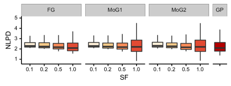
Figure 1: The distributions of sse and nlpd for a regression problem with a univariate Gaussian likelihood model on the boston housing dataset. Three approximate posteriors in savigp are used: fg (full Gaussian), mog1 (diagonal Gaussian), and mog2 (mixture of two diagonal Gaussians), along with various sparsity factors ($\text{SF}=M/N$). The smaller the sf the sparser the model, with $\text{SF}=1$ corresponding to the dense model. gp corresponds to the performance of exact inference using standard Gaussian process regression.

9.3.2 Warped Gaussian process

In warped Gaussian processes, the likelihood function is $p(y_{n}|f_{n})=\nabla_{y}t(y_{n})\mathcal{N}(t(y_{n});f_{n},\sigma^{2})$, for some transformation $t$. We used the same neural-net style transformation as Snelson et al. (2003), and evaluated the performance of our model on two datasets: creep (Cole et al., 2000), and abalone (Bache and Lichman, 2013). The results are compared with the performance of exact inference for warped Gaussian processes (wgp) described by Snelson et al. (2003), and also with the performance of exact Gaussian process inference with a univariate Gaussian likelihood model (gp). As shown in Figure 2, in the case of the abalone dataset, the performance is similar across all the models (fg, mog1 and mog2) and sparsity factors, and is comparable to the performance of the exact inference method for warped Gaussian processes (wgp). The results on creep are given in Appendix K.1.

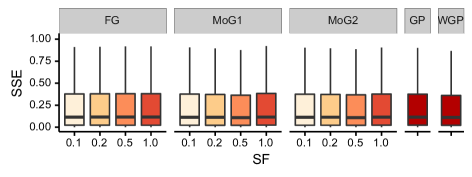
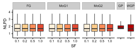
Figure 2: The distributions of sse and nlpd for a warped Gaussian process likelihood model on the abalone dataset. Three approximate posteriors in savigp are used: fg (full Gaussian), mog1 (diagonal Gaussian), and mog2 (mixture of two diagonal Gaussians), along with various sparsity factors ($\text{SF}=M/N$). The smaller the sf the sparser the model, with $\text{SF}=1$ corresponding to the non-sparse model. wgp corresponds to the performance of the exact inference method for warped Gaussian process models (Snelson et al., 2003), and gp is the performance of exact inference on a univariate Gaussian likelihood model.

9.3.3 Binary classification

For binary classification we used the logistic likelihood $p(y_{n}=1|f_{n})=1/(1+e^{-f_{n}})$ on the breast cancer dataset (Bache and Lichman, 2013) and compared our model against the expectation propagation (ep) and variational bounds (vbo) methods described by Nickisch and Rasmussen (2008). Results depicted in Figure 3 indicate that the error rate remains comparable across all models (fg, mog1, mog2) and sparsity factors, and is almost identical to the error rates obtained by inference using ep and vbo. Interestingly, the nlp shows more variation and generally degrades as the number of inducing points is increased, especially for mog1 and mog2 models, which can be attributed to the fact that these denser models are overly confident in their predictions.

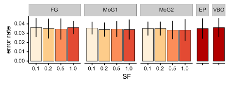
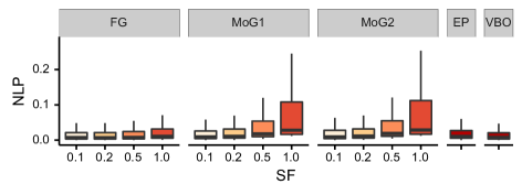
Figure 3: Error rates and nlp for binary classification using a logistic likelihood model on the Wisconsin breast cancer dataset. Three approximate posteriors are used: fg (full Gaussian), mog1 (diagonal Gaussian), and mog2 (mixture of two diagonal Gaussians), along with various sparsity factors ($\text{SF}=M/N$). The smaller the sf the sparser the model, with $\text{SF}=1$ corresponding to the original model without sparsity. The performance of inference using expectation propagation and variational bounds are denoted by ep and vbo respectively.

9.3.4 Multi-class classification

For multi-class classification, we used the softmax likelihood $p(y_{n}=c)=e^{-f_{c}}/\sum_{i}e^{-f_{i}}$, and trained the model to classify the digits 4, 7, and 9 from the usps dataset (Rasmussen and Williams, 2006). We compared our model against a variational inference method (vq) which represents the elbo using a quadratic lower bound on the likelihood terms (Khan et al., 2012). As we see in Figure 4, the error rates are slightly lower in denser fg models. We also note that all versions of savigp achieve comparable error rates to vq’s. Similarly to the binary classification case, nlp shows higher variation with higher sparsity factor, especially in mog1 and mog2 models.

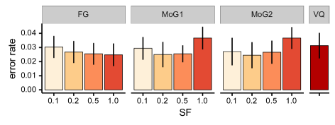
Figure 4: Classification error rates and nlp for the multi-class classification problem using a softmax likelihood model on the usps dataset. Three approximate posteriors in savigp are used: fg (full Gaussian), mog1 (diagonal Gaussian), and mog2 (mixture of two diagonal Gaussians), along with various sparsity factors ($\text{SF}=M/N$). The smaller the sf the sparser the model, with $\text{SF}=1$ corresponding to the original model without sparsity. vq corresponds to a variational inference method, which represents the elbo as a quadratic lower bound to the likelihood terms.

9.3.5 Log Gaussian Cox Process

The log Gaussian Cox process (lgcp) is an inhomogeneous Poisson process in which the log-intensity function is a shifted draw from a Gaussian process. Following Murray et al. (2010), we used the likelihood $p(y_{n}|f_{n})=\frac{\lambda^{y_{n}}_{n}\exp{(-\lambda_{n})}}{y_{n}!}$, where $\lambda_{n}=\exp{f_{n}+m}$ is the mean of a Poisson distribution and $m$ is the offset of the log mean. We applied savigp with the lgcp likelihood on a coal-mining disaster dataset (Jarrett, 1979), which can be seen in Figure 5 (top).

As baseline comparisons, we use hybrid Monte Carlo (hmc) and elliptical slice sampling (ess) described by Duane et al. (1987) and Murray et al. (2010) respectively. We collected every $100^{th}$ sample for a total of $10k$ samples after a burn-in period of $5k$ samples and used the Gelman-Rubin potential scale reduction factors (Gelman and Rubin, 1992) to check for convergence.

The bottom plot of Figure 5 shows the mean and variance of the predictions made by savigp, hmc and ess. We see that the fg model provides similar results across all sparsity factors, which is also comparable to the results provided by hmc and ess. mog1 and mog2 models provide the same mean as the fg models, but tend to underestimate the posterior variance. This under-estimation of posterior variance is well known for variational methods, especially under factorized posteriors. This results are more significant when comparing the running times across models. When using a slower Matlab implementation of our model, for a fair comparison across all methods, savigp was at least two orders of magnitude faster than hmc and one order of magnitude faster than ess.

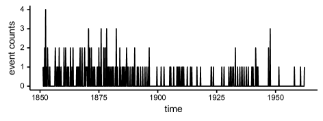
Figure 5: Top: the coal-mining disasters data. Bottom: the posteriors for a Log Gaussian Cox process on the data when using a fg (full Gaussian), mog1 (diagonal Gaussian), and mog2 (mixture of two diagonal Gaussians), along with various sparsity factors ($\text{SF}=M/N$). The smaller the sf the sparser the model, with $\text{SF}=1$ corresponding to non-sparse model. The solid line is the posterior mean and the shaded area represents 95% confidence intervals. hmc and ess correspond to hybrid Monte Carlo and elliptical slice sampling inference methods and are represented by orange dots and dashed green lines respectively.

9.4 Medium-scale Experiments

In this section we investigate the performance of savigp on four medium-scale problems on the datasets summarized in Table 2. Our goal here is to evaluate the model on medium-scale datasets, to study the effect of optimizing the inducing inputs, and to compare the performance of batch and stochastic optimization of the parameters. The first problem that we consider is multi-class classification of handwriting digits on the mnist dataset using a softmax likelihood model. The second problem uses the same dataset, but the task involves binary classification of odd and even digits using the logistic likelihood model. Therefore we refer to this dataset as the mnist binary dataset (mnist-b). The third problem uses the sarcos dataset (Vijayakumar and Schaal, 2000) and concerns an inverse-dynamics problem for a seven degrees-of-freedom sarcos anthropomorphic robot arm. The task is to map from a 21-dimensional input space (7 joint positions, 7 joint velocities, 7 joint accelerations) to the corresponding 7 joint torques. For this multi-output regression problem we use the Gaussian process regression network (gprn) likelihood model of Wilson et al. (2012), which allows for nonlinear models where the correlation between the outputs can be spatially adaptive. This is achieved by taking a linear combination of latent Gaussian processes, where the weights are also drawn from Gaussian processes. Finally, sarcos-2 is the same as sarcos, but the model is learned using only data from joints $4$ and $7$. For both sarcos and sarcos-2, the mean of the sse and nlpd across joints $4$ and $7$ are used for performance evaluation. We only consider joints $4$ and $7$ for sarcos, despite the fact that predictions are made across all $7$ joints to provide a direct comparison with sarcos-2 and with previous literature (Nguyen and Bonilla, 2014b). We also made use of automatic relevance determination (ard) for both the sarcos and sarcos-2 datasets.

Table 2: Datasets used on the medium-scale experiments. gprn stands for Gaussian process regression networks; $N_{train},N_{test},D$ are the number of training points, test points and input dimensions respectively; $Q$ is the number of latent processes; $P$ is the dimensionality of the output data; and ‘model’ is the model associated with the conditional likelihood used.

Dataset	$N_{train}$	$N_{test}$	$D$	$Q$	$P$	Model
mnist-b	60,000	10,000	784	1	1	Binary classification
mnist	60,000	10,000	784	10	10	Multi-class classification
sarcos-2	44,484	4,449	21	3	2	gprn (Wilson et al., 2012)
sarcos	44,484	4,449	21	8	7	gprn (Wilson et al., 2012)

9.4.1 Batch optimization

Classification.

Here we evaluate the performance of batch optimization of model parameters on multi-class classification using mnist and refer the reader to Appendix K.2 for the results on binary classification using mnist-b. We optimized the kernel hyperparameters and the variational parameters, but fixed the inducing point locations using $k$-means clustering. Unlike most previous approaches (Ranzato et al., 2006; Jarrett et al., 2009), we did not tune model parameters using the validation set. Instead, we considered the validation set to be part of the training set and used our variational framework to learn all model parameters. As such, the current setting likely provides a lower performance on test accuracy compared to the approaches that use a validation dataset, however our goal is simply to show that we were able to achieve competitive performance in a sparse setting when no knowledge of the likelihood model is used.

Figure 6 shows the result on the mnist dataset. we see that the performance improves with denser models. Overall, savigp achieves an error rate of $2.77\%$ at $\text{SF}=0.04$. This is a significant improvement over the results reported by Gal et al. (2014), in which a separate model was trained for each digit, which achieved an error rate of $5.95\%$. As a reference, previous literature reports about $12\%$ error rate by linear classifiers and less than $1\%$ error rate by state-of-the-art deep convolutional nets. Our results show that our method reduces the gap between gps and deep nets while solving the harder problem of full posterior estimation. In Appendix K.2 we show that our model can achieve slightly better performance than that reported by Hensman et al. (2015) on mnist-b.

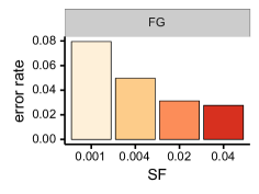
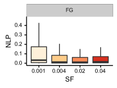
Figure 6: Error rates and nlp for multi-class classification on the mnist dataset. We used a full Gaussian (fg) posterior approximation across various sparsity factors ($\text{SF}=M/N$). The smaller the SF the sparser the model.

Gaussian process regression networks.

Figure 7 shows that sarcos-2 gets a significant benefit from a higher number of inducing points, which is consistent with previous work that found that the performance on this dataset improves as more data is being used to train the model (Vijayakumar and Schaal, 2000). The performance is significantly better than the results reported by Nguyen and Bonilla (2014b), who achieved a mean standardized squared eror (msse) of $0.2631$ and $0.0127$ across joints $4$ and $7$, against our values of $0.0033$ and $0.0065$ for $\text{SF}=0.04$. However, we note that their setting was much sparser than ours on joint $4$.

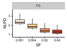
Figure 7: Mean sse and nlpd for multi-output regression on the sarcos-2 dataset. We used a full Gaussian (fg) posterior approximation across various sparsity factors ($\text{SF}=M/N$). The smaller the SF the sparser the model.

The results on sarcos (predicting on all joints) are given in Appendix K.3.

9.5 Inducing-input learning

We now compare the effect of adaptively learning the inducing inputs, versus initializing them using $k$-means and leaving them fixed. We look at the performance of our model under two settings: (i) a low number of inducing variables (SF$=0.001,0.004$) where the inducing inputs are learned, and (ii) a large number of inducing variables ($\text{SF}=0.02,0.04$) without learning of their locations.

Figure 8 shows the performance of the model under the two settings on mnist-b. We see that learning the location of the inducing variables yields a large gain in performance. In fact, the sparser models with inducing point learning performed similarly to the denser models, despite the fact that the two models differed by an order of magnitude when it came to the number of inducing variables. Additional results on mnist, sarcos and sarcos-2 are shown in Appendix K.4. Our analyses indicate that there is a trade-off between the reduction in computational complexity gained by reducing the number of inducing variables and the increased computational cost of calculating inducing-input gradients. As such, the advantage of learning the inducing inputs is dataset dependent and it is affected mainly by the input dimensionality ($D$).

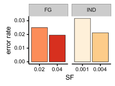
Figure 8: Comparison of error rate and nlp obtained by savigp without learning (fg) and with learning (ind) of inducing inputs for binary classification on the mnist-b dataset.

9.6 Batch Optimization vs Stochastic Optimization

In this section we compare the performance of our model after it has been trained in a batch setting versus a stochastic setting. We used adadelta as our stochastic optimization algorithm as it requires less hand-tuning than other algorithms such as vanilla stochastic gradient descend (sgd).

Table 3: Error rate (er) and negative log probability (nlp) obtained with savigp optimized using batch optimization (with l-bfgs) and stochastic optimization (with adadelta) on the mnist-b dataset. The inducing inputs are optimized in both cases.

Method	Batch $\text{SF}=0.001$	Batch $\text{SF}=0.004$	Stochastic $\text{SF}=0.001$	Stochastic $\text{SF}=0.004$
er	3.17%	2.12%	3.11%	2.68%
nlp	0.097	0.068	0.099	0.083

Table 3 shows only a slight deterioration in predictive performance on mnist-b when using stochastic optimization instead of batch optimization. In fact, our exploratory experiments showed that the error metrics could have significantly been reduced by meticulously hand-tuning momentum stochastic gradient descent (sgd). However, our goal was simply to show that our model does not suffer from a large loss in performance when going from a batch to a stochastic setting in medium-scale experiments, without requiring extensive hand tuning of the optimization algorithm. As we shall see in the next section, when batch optimization is not feasible, stochastic optimization in our model performs well when compared to state-of-the-art approaches for inference in gp models on very large datasets.

9.7 Large-scale Experiments

In this section we evaluate savigp on two large-scale problems involving prediction of airline delays (regression, $N=700,000$) and handwritten digit recognition (classification, $N=8,100,000$).

9.7.1 Airline delays

Here we consider the problem of predicting airline delays using a univariate Gaussian likelihood model (Hensman et al., 2013). We note that this dataset has outliers that can significantly affect the performance of regression algorithms when using metrics such as the rmse. This has also been pointed out by Das et al. (2015). Additionally, in order to match the application of the algorithms to a realistic setting, evaluation of learning algorithms on this dataset should always consider making predictions in the future. Therefore, unlike Hensman et al. (2013), we did not randomly select the training and test sets, instead we selected the first $700,000$ data points starting at a given offset as the training set and the next $100,000$ data points as the test set. We generated five training/test sets by setting the initial offset to $0$ and increasing it by $200,000$ each time.

We used the squared exponential covariance function with automatic relevance determination (ard), and optimized all the parameters using adadelta (Zeiler, 2012). We compare the performance of our model with the stochastic variational inference on gps method (svigp) described by Hensman et al. (2013), which assumes full knowledge of the likelihood function. Our method (savigp) and svigp were optimized using adadelta with identical settings. We also report the results of Bayesian linear regression with a zero-mean unit-variance prior over the weights (linear) and Gaussian process regression using subsets of the training data (gp1000 and gp2000 using $1,000$ and $2,000$ datapoints respectively). For each run we fit gp1000 and gp2000 ten times using a randomly selected subset of the training data. Kernel hyper-parameters of gp1000 and gp2000 were optimized using l-bfgs.

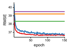
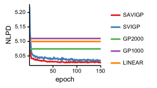
Figure 9: The rmse (left) and nlpd (right) of svigp (Hensman et al., 2013), and savigp (our method) averaged across all $5$ airline-delay experiment runs. The x-axis represents the number of passes over the data (epochs). The figure also shows the performance of gp1000, gp2000 and Bayesian linear regression (linear) after training is completed.

Figure 9 shows the performance of savigp and the four baselines. We see that savigp converges at a very similar rate to svigp, despite making no assumption about the likelihood model. Furthermore, savigp performs better than all three simple baselines after less than $5$ epochs. We note that our results are not directly comparable with those reported by Hensman et al. (2013), since we deal with the harder problem of predicting future events due to the way our dataset is selected.

9.7.2 Training Loss vs Test Performance

An additional interesting question about the behavior of our model relates to how well the training objective function correlates to the test error metrics. Figure 10 shows how the performance metrics (rmse and nlpd) on the test data vary along with the negative evidence lower bound (nelbo). As we can see, changes in the nelbo closely mirror changes in rmse and nlpd in our model, which is an indication that the variational objective generalizes well to test performance when using these metrics.

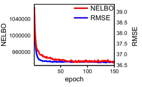
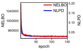
Figure 10: The rmse (left) and nlpd (right) of savigp on the test data alongside the negative evidence lower bound (nelbo) on the training data, averaged over five runs of the airline-delay experiment.

9.7.3 Large-scale mnist

In this section we evaluate the performance of savigp on the mnist8m (Loosli et al., 2007) dataset, which artificially extends the mnist dataset to 8.1 million training points by pseudo-randomly transforming existing mnist images.

We train savigp on the mnist8m dataset by optimizing only variational parameters stochastically, with a batch size of $1000$ and $2000$ inducing points. We also use a squared exponential covariance function without automatic relevance determination.

After optimizing the model for $19$ hours, we observe an error rate of $1.54\%$ on the test set and lower, middle and upper nlp quartiles of $8.61\mathrm{e}{-4}$, $3.81\mathrm{e}{-3}$, and $2.16\mathrm{e}{-2}$ respectively. We see that this outperforms significantly our previous result in §9.4 on standard mnist, where we reported an error rate of $2.77\%$. As a point of comparison with hard-coded approaches, Henao and Winther (2012) reported 0.86% error rate on mnist when considering an augmented active set (which is analogous to the concept of inducing inputs/variables) and a 9th-degree polynomial covariance function.

Finally, Figure 11 shows the training loss (the nelbo) of savigp on mnist8m as a function of the number of training steps, where we note that the loss decreases rapidly in the first 2,000 iterations and stabilizes at around 4,000 iterations.

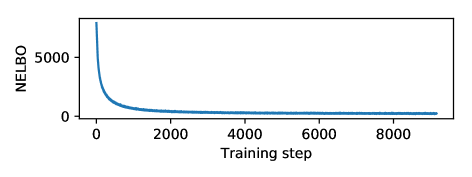
Figure 11: The negative evidence lower bound (nelbo) on the current batch of the mnist8m training set over time on savigp. The x-axis represents the number of training steps taken.

9.8 Seismic inversion

In this experiment we aim to evaluate our method qualitatively on a non-standard inference problem motivating the need for black-box likelihoods. This application considers a one-dimensional seismic inversion and was investigated by Bonilla et al. (2016). Given noisy surface observations of sound-reflection times, the goal is to infer the geometry (layer depths) of subsurface geological layers and seismic propagation velocities within each layer. For this, we consider a real dataset from a seismic survey carried out in the Otway basin region in the state of Victoria, Australia.

Setting

There are $N=113$ site locations with $P=4$ interface reflections (layers) per site. The inputs are given by the surface locations of the seismic sensors ($\mathbf{X}$), the outputs are the observed times at the different locations for each of the layers ($\mathbf{Y}$) and we aim to infer $Q=2*P$ latent functions, i.e. $P$ functions corresponding to layer depths and $P$ functions corresponding to seismic propagation velocities. For clarity, in this section we refer to the latent functions corresponding to depth and velocity as $f^{\text{d}}$ and $f^{\text{v}}$, respectively.

Likelihood

The likelihood of the observed times $y_{np}$ for location $\mathbf{x}_{n}$ and interface $p$ is given by:

$$y_{np}=\left\{\begin{array}[]{ll}2\left(\frac{f^{\text{d}}_{np}}{f^{\text{v}}_{np}}\right)+\epsilon_{np},&\text{ for }p=1,\\ 2\left(\frac{f^{\text{d}}_{np}-f^{\text{d}}_{np-1}}{f^{\text{v}}_{np}}\right)+y_{np-1}+\epsilon_{np},&\text{ for }1<p\leq P\text{,}\end{array}\right.$$ (43)

where $\epsilon_{np}\sim\mathcal{N}(0,\sigma^{2}_{p})$ and $\sigma^{2}_{p}$ is the output-dependent noise variance. As in Bonilla et al. (2016), we set the corresponding standard deviations to 0.025s, 0.05s, 0.075s and 0.1s.

Prior setting:

We used the same prior as in Bonilla et al. (2016), with prior mean depths of 200m, 500m, 1600m and 2200m and prior mean velocities of 1950m/s, 2300m/s, 2750m/s and 3650m/s. The corresponding standard deviations for the depths were set to 15% of the layer mean, and for the velocities they were set to 10% of the layer mean. A squared exponential covariance function with unit length-scale was used.

Posterior estimation

We ran our algorithm for the dense case ($\mathbf{Z}=\mathbf{X}$) using a full Gaussian posterior and batch optimization, initializing the posterior means to the prior means and the posterior covariance to a diagonal matrix with entries corresponding to $0.1\%$ of the prior variances. The results are given in Figure 12, where we see that savigp’s posterior closely match the “true” posterior obtained by the mcmc algorithm developed in Bonilla et al. (2016), although the variances are overestimated, which can be see as a consequence of our variational approach using a full Gaussian approximate posterior.

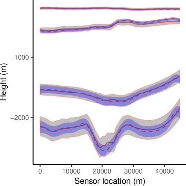
Figure 12: Results for the seismic inversion experiment using our algorithm (savigp) and the mcmc algorithm developed by Bonilla et al. (2016). The mean and standard deviations envelopes are shown for savigp and mcmc in solid and dashed lines, respectively. Left: inferred layer boundaries. Right: inferred seismic velocities.

10 Conclusions and Discussion

We have developed scalable automated variational inference for Gaussian process models (savigp), an inference method for models with Gaussian process (gp) priors, multiple outputs, and nonlinear likelihoods. The method is generally applicable to black-box likelihoods, i.e. it does not need to know the details of the conditional likelihood (or its gradients), only requiring its evaluation as a black-box function.

One of the key properties of this method is that, despite using a flexible variational posterior such as a mixture-of-Gaussians distribution, it is statistically efficient in that it requires samples from univariate Gaussian distributions to estimate the evidence lower bound (elbo) and its gradients.

In order to provide scalability to very large datasets, we have used an augmented prior via the so-called inducing variables, which are prevalent in most sparse gp approximations. This has allowed us to decompose the elbo as a sum of terms over the datapoints, hence giving way for the application of stochastic optimization and parallel computation.

Our small-scale experiments have shown that savigp can perform as accurately as solutions that have been hard-coded specifically for the conditional likelihood of the problem at hand, even under high sparsity levels.

Our medium-scale experiments also have shown the effectiveness of savigp, when considering problems such as multi-class classification on the mnist dataset and highly nonlinear likelihoods such as that used in gprn. On these experiments, we also have analyzed the effect of learning the inducing inputs, i.e. the locations corresponding to the inducing variables, and concluded that doing this can yield significant improvements in performance, reducing the numbers of inducing variables required to achieve similar accuracy by an order of magnitude. Nevertheless, there is generally a trade-off between reducing the time cost gained by having a lower number of inducing inputs and the overhead of carrying out optimization over these locations.

Our first large-scale experiment, on the problem of predicting airline delays, showed that savigp is on par with the state-of-the-art approach for Gaussian process regression on big data (Hensman et al., 2013). In fact, our results show that savigp is slightly better but we attribute those differences to implementation specifics. The important message is that savigp can attain state-of-the-art performance even without exploiting specific knowledge of the likelihood model. Our second large-scale experiment shows that having an inference algorithm for gp models with non-Gaussian likelihood for large datasets is worthwhile, as the performance obtained on mnist8m (using 8.1M observations) was significantly better than on the standard mnist (using 60K observations).

Our final experiment considered a non-standard inference problem concerning a seismic inversion task. In this problem savigp yielded a solution for the posterior over latent functions that closely matched the solution obtained by a (non-scalable) sampling algorithm.

Overall, we believe savigp has the potential to be a powerful tool for practitioners and researchers when devising models for new or existing problems with Gaussian process priors for which variational inference is not yet available. As mentioned in Section 2, we are very much aware of recent developments in the areas of probabilistic programming, stochastic variational inference and Bayesian deep learning. Advances such as those in black-box variational inference (bbvi, Ranganath et al., 2014) and variational auto-encoders (Rezende et al., 2014; Kingma and Welling, 2014) are incredibly exciting for the machine learning community. While the former, bbvi, is somewhat too general to be useful in practice for gp models, the latter (variational auto-encoders) requires specific knowledge of the likelihood and is not a truly black-box method.

Finally, we are working on extending our models to more complex settings such as structured prediction problems, i.e. where the conditional likelihood is a non-iid model such as a chain or a tree (see e.g. Galliani et al., 2017, for a recent reference). Such settings provide incredible challenges from the computational and modeling perspectives. For example, how to deal with the exponential increase in the number of parameters of the model, and how to reduce the number of calls to an expensive conditional likelihood model. We believe that the benefits of being Bayesian well outweigh the effort in exploring such challenges.

Acknowledgments

We acknowledge the contribution by Trung V. Nguyen to the original conference paper (Nguyen and Bonilla, 2014a). evb started this work at the University of New South Wales (unsw sydney) and was partially supported by unsw’s Faculty of Engineering Research Grant Program project # PS37866; unsw’s Academic Start-Up Funding Scheme project # PS41327; and an aws in Education Research Grant award. AD started this work at unsw sydney, and was supported by a Research Fellowship from unsw sydney.

Appendix A Derivation of the KL-divergence Term

Here we derive the expressions for the terms composing the KL-divergence ($\mathcal{L}_{\text{kl}}=\mathcal{L}_{\text{ent}}+\mathcal{L}_{\text{cross}}$) part of the log-evidence lower bound ($\mathcal{L}_{\text{elbo}}$).

The entropy term is given by:

$$\mathcal{L}_{\text{ent}}(\boldsymbol{\lambda}) =-\mathbb{E}_{q(\mathbf{u}|\boldsymbol{\lambda})}{\left[\log q(\mathbf{u}|\boldsymbol{\lambda})\right]}$$ (44)

$$=-\int\sum_{k=1}^{K}\pi_{k}q_{k}(\mathbf{u}|\mathbf{m}_{k},\mathbf{S}_{k})\log\sum_{\ell=1}^{K}\pi_{\ell}q_{\ell}(\mathbf{u}|\mathbf{m}_{\ell},\mathbf{S}_{\ell})\text{d}\mathbf{u}$$ (45)

$$=-\sum_{k=1}^{K}\pi_{k}\int\mathcal{N}(\mathbf{u};\mathbf{m}_{k},\mathbf{S}_{k})\log\sum_{\ell=1}^{K}\pi_{\ell}\mathcal{N}(\mathbf{u};\mathbf{m}_{\ell},\mathbf{S}_{\ell})\text{d}\mathbf{u}$$ (46)

$$\geq-\sum_{k=1}^{K}\pi_{k}\log\int\mathcal{N}(\mathbf{u};\mathbf{m}_{k},\mathbf{S}_{k})\sum_{\ell=1}^{K}\pi_{\ell}\mathcal{N}(\mathbf{u}|\mathbf{m}_{\ell},\mathbf{S}_{\ell})\text{d}\mathbf{u}$$ (47)

$$=-\sum_{k=1}^{K}\pi_{k}\log\sum_{\ell=1}^{K}\pi_{\ell}\int\mathcal{N}(\mathbf{u};\mathbf{m}_{k},\mathbf{S}_{k})\mathcal{N}(\mathbf{u}|\mathbf{m}_{\ell},\mathbf{S}_{\ell})\text{d}\mathbf{u}$$ (48)

$$=-\sum_{k=1}^{K}\pi_{k}\log\sum_{\ell=1}^{K}\pi_{\ell}\mathcal{N}(\mathbf{m}_{k};\mathbf{m}_{\ell},\mathbf{S}_{k}+\mathbf{S}_{\ell})\stackrel{{\scriptstyle\text{\tiny def}}}{{=}}\widehat{\mathcal{L}}_{\text{ent}}\text{,}$$ (49)

where we have used Jensen’s inequality to bring the logarithm out of the integral from Equations (46) to (47).

The negative cross-entropy term can be computed as:

$$\mathcal{L}_{\text{cross}}(\boldsymbol{\lambda}) =\mathbb{E}_{q(\mathbf{u}|\boldsymbol{\lambda})}{\left[\log p(\mathbf{u})\right]}=\sum_{k=1}^{K}\int\pi_{k}q_{k}(\mathbf{u}|\boldsymbol{\lambda}_{k})\log p(\mathbf{u})\text{d}\mathbf{u}$$ (50)

$$=\sum_{k=1}^{K}\sum_{j=1}^{Q}\pi_{k}\int\mathcal{N}(\mathbf{u}_{j};\mathbf{m}_{kj},\mathbf{S}_{kj})\log\mathcal{N}(\mathbf{u}_{j};\mathbf{0},\mathbf{K}_{\mathbf{z}\mathbf{z}}^{j})\text{d}\mathbf{u}_{j}$$ (51)

$$=\sum_{k=1}^{K}\sum_{j=1}^{Q}\pi_{k}\left[\log\mathcal{N}(\mathbf{m}_{kj};\mathbf{0},\mathbf{K}_{\mathbf{z}\mathbf{z}}^{j})-\frac{1}{2}\mbox{ \rm tr }(\mathbf{K}_{\mathbf{z}\mathbf{z}}^{j})^{-1}\mathbf{S}_{kj}\right]$$ (52)

$$=-\frac{1}{2}\sum_{k=1}^{K}\pi_{k}\sum_{j=1}^{Q}\left[M\log 2\pi+\log\left\lvert\mathbf{K}_{\mathbf{z}\mathbf{z}}^{j}\right\rvert+\mathbf{m}_{kj}^{T}(\mathbf{K}_{\mathbf{z}\mathbf{z}}^{j})^{-1}\mathbf{m}_{kj}+\mbox{ \rm tr }(\mathbf{K}_{\mathbf{z}\mathbf{z}}^{j})^{-1}\mathbf{S}_{kj}\right]\text{.}$$ (53)

Appendix B Proof of Theorem 1

In this section we prove Theorem 1 concerning the statistical efficiency of the estimator of the expected log likelihood and its gradients, i.e. that both can be estimated using expectations over Univariate Gaussian distributions.

B.1 Estimation of $\mathcal{L}_{\text{ell}}$

Taking the original expression in Equation (20) we have that:

$$\mathcal{L}_{\text{ell}}(\boldsymbol{\lambda}) =\mathbb{E}_{q(\mathbf{f}|\boldsymbol{\lambda})}{\left[\log p(\mathbf{y}|\mathbf{f},\boldsymbol{\phi})\right]}\text{,}$$ (54)

$$=\sum_{n=1}^{N}\int_{\mathbf{f}}{q(\mathbf{f}|\boldsymbol{\lambda})}{\log p(\mathbf{y}_{n}|\mathbf{f}_{n\cdot},\boldsymbol{\phi})}\text{d}\mathbf{f}\text{,}$$ (55)

$$=\sum_{n=1}^{N}\int_{\mathbf{f}_{n\cdot}}\int_{\mathbf{f}_{\neg n\cdot}}q(\mathbf{f}_{\neg n\cdot}|\mathbf{f}_{n\cdot})q(\mathbf{f}_{n\cdot})\log p(\mathbf{y}_{n}|\mathbf{f}_{n\cdot},\boldsymbol{\phi})\text{d}\mathbf{f}_{\neg n\cdot}\text{d}\mathbf{f}_{n\cdot}\text{,}$$ (56)

$$=\sum_{n=1}^{N}\mathbb{E}_{q_{(n)}(\mathbf{f}_{n\cdot})}{\left[\log p(\mathbf{y}_{n}|\mathbf{f}_{n\cdot},\boldsymbol{\phi})\right]}\text{,}$$ (57)

$$=\sum_{n=1}^{N}\sum_{k=1}^{K}\pi_{k}\mathbb{E}_{q_{k(n)}(\mathbf{f}_{n\cdot}|\boldsymbol{\lambda}_{k})}{\left[\log p(\mathbf{y}_{n}|\mathbf{f}_{n\cdot},\boldsymbol{\phi})\right]}\text{,}$$ (58)

where we have applied the linear property of the expectation operation in Equation (55); used $\mathbf{f}_{\neg n\cdot}$ to denote all the latent functions except those corresponding to the n$\mathrm{th}$ observation, and integrated these out to obtain Equation (57); and used the form of the marginal posterior (mog in Equation (21)) to get Equation (58).

As described in Section 4.6, $q_{k(n)}(\mathbf{f}_{n\cdot}|\boldsymbol{\lambda}_{k})$ is a $Q$-dimensional Gaussian with diagonal covariance, hence computation of Equation (58) only requires expectations over univariate Gaussian distributions. $\blacksquare$

B.2 Estimation of the Gradients of $\mathcal{L}_{\text{ell}}$

Denoting the k$\mathrm{th}$ term for the n$\mathrm{th}$ observation of the expected log likelihood with $\mathcal{L}_{\text{ell}}^{(k,n)}$ we have that:

$$\mathcal{L}_{\text{ell}}^{(k,n)} =\mathbb{E}_{q_{k(n)}(\mathbf{f}_{n\cdot}|\boldsymbol{\lambda}_{k})}{\left[\log p(\mathbf{y}_{n}|\mathbf{f}_{n\cdot},\boldsymbol{\phi})\right]}$$ (59)

$$=\int_{\mathbf{f}_{n\cdot}}q_{k(n)}(\mathbf{f}_{n\cdot}|\boldsymbol{\lambda}_{k})\log p(\mathbf{y}_{n}|\mathbf{f}_{n\cdot},\boldsymbol{\phi})\text{d}\mathbf{f}_{n\cdot}$$ (60)

$$\nabla_{\boldsymbol{\lambda}_{k}}\mathcal{L}_{\text{ell}}^{(k,n)} =\int_{\mathbf{f}_{n\cdot}}q_{k(n)}(\mathbf{f}_{n\cdot}|\boldsymbol{\lambda}_{k})\nabla_{\boldsymbol{\lambda}_{k}}\log q_{k(n)}(\mathbf{f}_{n\cdot}|\boldsymbol{\lambda}_{k})\log p(\mathbf{y}_{n}|\mathbf{f}_{n\cdot},\boldsymbol{\phi})\text{d}\mathbf{f}_{n\cdot}$$ (61)

$$=\mathbb{E}_{q_{k(n)}(\mathbf{f}_{n\cdot}|\boldsymbol{\lambda}_{k})}{\left[\nabla_{\boldsymbol{\lambda}_{k}}\log q_{k(n)}(\mathbf{f}_{n\cdot}|\boldsymbol{\lambda}_{k})\log p(\mathbf{y}_{n}|\mathbf{f}_{n\cdot},\boldsymbol{\phi})\right]}\text{,}$$ (62)

for $\boldsymbol{\lambda}_{k}\in\{\mathbf{m}_{k},\mathbf{S}_{k}\}$, and for the mixture proportions the gradients can be estimated straightforwardly using Equation (26). We have used in Equation (61) the fact that $\nabla_{\mathbf{x}}f(\mathbf{x})=f(\mathbf{x})\nabla_{\mathbf{x}}\log f(\mathbf{x})$ for any nonnegative function $f(\mathbf{x})$. We see that our resulting gradient estimate has an analogous form to that obtained in Equation (58), hence its computation only requires expectations over univariate Gaussian distributions. $\blacksquare$

Appendix C Gradients of the Evidence Lower Bound wrt Variational Parameters

Here we specify the gradients of the log-evidence lower bound ($\mathcal{L}_{\text{elbo}}$) wrt variational parameters. For the covariance, we consider $\mathbf{S}_{kj}$ of general structure but also give the updates when $\mathbf{S}_{kj}$ is a diagonal matrix, denoted with $\tilde{\mathbf{S}}_{kj}$.

C.1 KL-divergence Term

Let $\mathbf{K}_{zz}$ be the block-diagonal covariance with $Q$ blocks $\mathbf{K}_{\mathbf{z}\mathbf{z}}^{j}$, $j=1,\ldots Q$. Additionally, let us assume the following definitions:

$$\mathbf{C}_{kl} \stackrel{{\scriptstyle\text{\tiny def}}}{{=}}\mathbf{S}_{k}+\mathbf{S}_{\ell}\text{,}$$ (63)

$$\mathcal{N}_{k\ell} \stackrel{{\scriptstyle\text{\tiny def}}}{{=}}\mathcal{N}(\mathbf{m}_{k};\mathbf{m}_{\ell},\mathbf{C}_{kl})\text{,}$$ (64)

$$z_{k} \stackrel{{\scriptstyle\text{\tiny def}}}{{=}}\sum_{\ell=1}^{K}\pi_{\ell}\mathcal{N}_{k\ell}\text{.}$$ (65)

The gradients of $\mathcal{L}_{\text{kl}}$ wrt the posterior mean and posterior covariance for component $k$ are:

$$\nabla_{\mathbf{m}_{k}}\mathcal{L}_{\text{cross}} =-\pi_{k}\mathbf{K}^{-1}_{zz}\mathbf{m}_{k}\text{,}$$ (66)

$$\nabla_{\mathbf{S}_{k}}\mathcal{L}_{\text{cross}} =-\frac{1}{2}\pi_{k}\mathbf{K}^{-1}_{zz}\text{, and for diagonal covariance we have:}$$ (67)

$$\nabla_{\tilde{\mathbf{S}}_{k}}\mathcal{L}_{\text{cross}} =-\frac{1}{2}\pi_{k}\operatorname{diag}(\mathbf{K}^{-1}_{zz})\text{,}$$ (68)

$$\ \nabla_{\pi_{k}}\mathcal{L}_{\text{cross}} =-\frac{1}{2}\sum_{j=1}^{Q}[M\log 2\pi+\log\left\lvert\mathbf{K}_{\mathbf{z}\mathbf{z}}^{j}\right\rvert+\mathbf{m}_{kj}^{T}(\mathbf{K}_{\mathbf{z}\mathbf{z}}^{j})^{-1}\mathbf{m}_{kj}+\mbox{ \rm tr }{(\mathbf{K}_{\mathbf{z}\mathbf{z}}^{j})^{-1}\mathbf{S}_{kj}}]\text{,}$$ (69)

where we note that we compute $\mathbf{K}^{-1}_{zz}$ by inverting the corresponding blocks $\mathbf{K}_{\mathbf{z}\mathbf{z}}^{j}$ independently. The gradients of the entropy term wrt the variational parameters are:

$$\nabla_{\mathbf{m}_{k}}\widehat{\mathcal{L}}_{\text{ent}} =\pi_{k}\sum_{\ell=1}^{K}\pi_{\ell}\left(\frac{\mathcal{N}_{k\ell}}{z_{k}}+\frac{\mathcal{N}_{k\ell}}{z_{\ell}}\right)\mathbf{C}_{kl}^{-1}(\mathbf{m}_{k}-\mathbf{m}_{\ell})\text{,}$$ (70)

$$\nabla_{\mathbf{S}_{k}}\widehat{\mathcal{L}}_{\text{ent}} =\frac{1}{2}\pi_{k}\sum_{\ell=1}^{K}\pi_{\ell}\left(\frac{\mathcal{N}_{k\ell}}{z_{k}}+\frac{\mathcal{N}_{k\ell}}{z_{\ell}}\right)\left[\mathbf{C}_{kl}^{-1}-\mathbf{C}_{kl}^{-1}(\mathbf{m}_{k}-\mathbf{m}_{\ell})(\mathbf{m}_{k}-\mathbf{m}_{\ell})^{T}\mathbf{C}_{kl}^{-1}\right]\text{,}$$ (71)

and for diagonal covariance we have:

$$\nabla_{\tilde{\mathbf{S}}_{k}}\widehat{\mathcal{L}}_{\text{ent}} =\frac{1}{2}\pi_{k}\sum_{\ell=1}^{K}\pi_{\ell}\left(\frac{\mathcal{N}_{k\ell}}{z_{k}}+\frac{\mathcal{N}_{k\ell}}{z_{\ell}}\right)\left[\tilde{\mathbf{C}}_{kl}^{-1}-\tilde{\mathbf{C}}_{kl}^{-1}\operatorname{diag}\left((\mathbf{m}_{k}-\mathbf{m}_{\ell})\odot(\mathbf{m}_{k}-\mathbf{m}_{\ell})\right)\tilde{\mathbf{C}}_{kl}^{-1}\right]\text{,}$$ (72)

$$\nabla_{\pi_{k}}\widehat{\mathcal{L}}_{\text{ent}} =-\log z_{k}-\sum_{\ell=1}^{K}\pi_{\ell}\frac{\mathcal{N}_{k\ell}}{z_{\ell}}\text{,}$$ (73)

where $\tilde{\mathbf{C}}_{kl}$ is the diagonal matrix defined analogously to $\mathbf{C}_{kl}$ in Equation (63) and $\odot$ is the Hadamard product.

C.2 Expected Log Likelihood Term

Monte Carlo estimates of the gradients of the expected log likelihood term are:

$$\nabla{\mathbf{m}_{kj}}\widehat{\mathcal{L}}_{\text{ell}} =\frac{\pi_{k}}{S}(\mathbf{K}_{\mathbf{z}\mathbf{z}}^{j})^{-1}\sum_{n=1}^{N}{\mathbf{k}_{\mathbf{z}n}^{j}}{[\mathbf{\Sigma}_{k(n)}]^{-1}_{j,j}}\sum_{i=1}^{S}\left(f_{nj}^{(k,i)}-{[\mathbf{b}_{k(n)}]_{j}}\right)\log p(\mathbf{y}_{n}|\mathbf{f}_{n\cdot}^{(k,i)})\text{,}$$ (74)

$$\nabla{\mathbf{S}_{kj}}\widehat{\mathcal{L}}_{\text{ell}} =\frac{\pi_{k}}{2S}\sum_{n=1}^{N}\left(\mathbf{a}_{jn}\mathbf{a}_{jn}^{T}\right)\sum_{i=1}^{S}\left[{[\mathbf{\Sigma}_{k(n)}]^{-2}_{j,j}}\left(f_{nj}^{(k,i)}-{[\mathbf{b}_{k(n)}]_{j}}\right)^{2}-{[\mathbf{\Sigma}_{k(n)}]^{-1}_{j,j}}\right]\log p(\mathbf{y}_{n}|\mathbf{f}_{n\cdot}^{(k,i)})\text{,}$$ (75)

$$\nabla{\pi_{k}}\widehat{\mathcal{L}}_{\text{ell}} =\frac{1}{S}\sum_{n=1}^{N}\sum_{i=1}^{S}\log p(\mathbf{y}_{n}|\mathbf{f}_{n\cdot}^{(k,i)})\text{,}$$ (76)

and for diagonal covariance $\tilde{\mathbf{S}}_{kj}$ we replace $\left(\mathbf{a}_{jn}\mathbf{a}_{jn}^{T}\right)$ with $\operatorname{diag}\left(\mathbf{a}_{jn}\odot\mathbf{a}_{jn}\right)$ in Equation (75), where $\odot$ is the Hadamard product and $\operatorname{diag}(\mathbf{v})$ takes the input vector $\mathbf{v}$ and outputs a matrix with $\mathbf{v}$ on its diagonal. We have also defined above ${\mathbf{k}_{\mathbf{z}n}^{j}}\stackrel{{\scriptstyle\text{\tiny def}}}{{=}}\kappa_{j}(\mathbf{Z}_{j},\mathbf{x}_{n})$, i.e. the vector obtained from evaluating the covariance function $j$ between the inducing points $\mathbf{Z}_{j}$ and datapoint $\mathbf{x}_{n}$.

Appendix D Gradients of the Evidence Lower Bound wrt Covariance Hyperparameters and Likelihood Parameters

Here we give the gradients of the variational objective ($\mathcal{L}_{\text{elbo}}$) wrt the covariance hyperparameters and, when required, the conditional likelihood parameters. We note here that our method does not require gradients of the conditional likelihood $p(\mathbf{y}|\mathbf{f},\boldsymbol{\phi})$ wrt the latent functions $\mathbf{f}$. However, if the conditional likelihood is parametrized by $\boldsymbol{\phi}$ and point-estimates of these parameters are needed, these can also be learned in our variational framework.

D.1 Covariance Hyperparameters

The gradients of the terms in the KL-divergence part of $\mathcal{L}_{\text{elbo}}$ wrt a covariance hyperparameter $\theta_{j}$ are:

$$\nabla_{\theta_{j}}\widehat{\mathcal{L}}_{\text{ent}} =0\text{,}$$ (77)

$$\nabla_{\theta_{j}}\mathcal{L}_{\text{cross}} =-\frac{1}{2}\sum_{k=1}^{K}\pi_{k}\mbox{ \rm tr }\big{[}(\mathbf{K}_{\mathbf{z}\mathbf{z}}^{j})^{-1}\nabla_{\theta_{j}}\mathbf{K}_{\mathbf{z}\mathbf{z}}^{j}$$ (78)

$$\qquad\qquad\qquad-(\mathbf{K}_{\mathbf{z}\mathbf{z}}^{j})^{-1}\nabla_{\theta_{j}}\mathbf{K}_{\mathbf{z}\mathbf{z}}^{j}(\mathbf{K}_{\mathbf{z}\mathbf{z}}^{j})^{-1}\left(\mathbf{m}_{kj}\mathbf{m}_{kj}^{T}+\mathbf{S}_{j}\right)\big{]}\text{.}$$

For the $\widehat{\mathcal{L}}_{\text{ell}}$ we have that:

$$\nabla_{\theta_{j}}\widehat{\mathcal{L}}_{\text{ell}}=\sum_{n=1}^{N}\sum_{k=1}^{K}\pi_{k}\mathbb{E}_{q_{k(n)}(\mathbf{f}_{n\cdot}|\boldsymbol{\lambda}_{k})}{\left[\nabla_{\theta_{j}}\log q_{k(n)}(\mathbf{f}_{n\cdot}|\boldsymbol{\lambda}_{k})\log p(\mathbf{y}_{n}|\mathbf{f}_{n\cdot})\right]}\text{,}$$ (79)

and computing the corresponding gradient we obtain:

$$\nabla_{\theta_{j}}\widehat{\mathcal{L}}_{\text{ell}}=-\frac{1}{2}\sum_{n=1}^{N}\sum_{k=1}^{K} \pi_{k}\mathbb{E}_{q_{k(n)}(\mathbf{f}_{n\cdot}|\boldsymbol{\lambda}_{k})}\Big{[}\Big{(}{[\mathbf{\Sigma}_{k(n)}]^{-1}_{j,j}}\nabla_{\theta_{j}}{[\mathbf{\Sigma}_{k(n)}]_{j,j}}$$ (80)

$$-2(f_{nj}-{[\mathbf{b}_{k(n)}]_{j}}){[\mathbf{\Sigma}_{k(n)}]^{-1}_{j,j}}\nabla_{\theta_{j}}{[\mathbf{b}_{k(n)}]_{j}}$$

$$-(f_{nj}-{[\mathbf{b}_{k(n)}]_{j}})^{2}{[\mathbf{\Sigma}_{k(n)}]^{-2}_{j,j}}\nabla_{\theta_{j}}{[\mathbf{\Sigma}_{k(n)}]_{j,j}}\Big{)}\log p(\mathbf{y}_{n}|\mathbf{f}_{n\cdot})\Big{]}\text{,}$$

for which we need:

$$\nabla_{\theta_{j}}{[\mathbf{b}_{k(n)}]_{j}} =\left(\nabla_{\theta_{j}}\mathbf{a}_{jn}^{T}\right)\mathbf{m}_{kj}\text{,}$$ (81)

$$\nabla_{\theta_{j}}{[\mathbf{\Sigma}_{k(n)}]_{j,j}} =\nabla_{\theta_{j}}{[\widetilde{\mathbf{K}}_{j}]_{n,n}}+2\left(\nabla_{\theta_{j}}\mathbf{a}_{jn}^{T}\right)\mathbf{S}_{kj}\mathbf{a}_{jn}$$ (82)

$$=\nabla_{\theta_{j}}\kappa(\mathbf{x}_{n},\mathbf{x}_{n})-\left(\nabla_{\theta_{j}}\mathbf{a}_{jn}^{T}\right){\mathbf{k}_{\mathbf{z}n}^{j}}-\mathbf{a}_{jn}^{T}\nabla_{\theta_{j}}{\mathbf{k}_{\mathbf{z}n}^{j}}$$ (83)

$$\qquad+2\left(\nabla_{\theta_{j}}\mathbf{a}_{jn}^{T}\right)\mathbf{S}_{kj}\mathbf{a}_{jn}\text{,}$$ (84)

where

$$\nabla_{\theta_{j}}\mathbf{a}_{jn}^{T}=\Big{(}\nabla_{\theta_{j}}({\mathbf{k}_{\mathbf{z}n}^{j}})^{T}-\mathbf{a}_{jn}^{T}\nabla_{\theta_{j}}\mathbf{K}_{\mathbf{z}\mathbf{z}}^{j}\Big{)}(\mathbf{K}_{\mathbf{z}\mathbf{z}}^{j})^{-1}\text{,}$$ (85)

and as in the main text we have defined $\mathbf{a}_{jn}\stackrel{{\scriptstyle\text{\tiny def}}}{{=}}[{\mathbf{A}_{j}}]_{:,n}$, i.e. the vector corresponding to the n$\mathrm{th}$ column of $\mathbf{A}_{j}$. Furthermore, as in the previous section, ${\mathbf{k}_{\mathbf{z}n}^{j}}\stackrel{{\scriptstyle\text{\tiny def}}}{{=}}\kappa_{j}(\mathbf{Z}_{j},\mathbf{x}_{n})$.

D.2 Likelihood Parameters

Since the terms in the KL-divergence do not depend on the likelihood parameters we have that $\nabla_{\boldsymbol{\phi}}\widehat{\mathcal{L}}_{\text{ent}}=\nabla_{\boldsymbol{\phi}}\mathcal{L}_{\text{cross}}=0$. For the gradients of the expected log likelihood term we have that:

$$\nabla_{\boldsymbol{\phi}}{\widehat{\mathcal{L}}_{\text{ell}}}=\frac{1}{S}\sum_{n=1}^{N}\sum_{k=1}^{K}\pi_{k}\sum_{i=1}^{S}\nabla_{\boldsymbol{\phi}}\log p(\mathbf{y}_{n}|\mathbf{f}_{n\cdot}^{(k,i)},\boldsymbol{\phi})\text{,}$$ (86)

where $\{\mathbf{f}_{n\cdot}^{(k,i)}\}\sim\mathcal{N}(\mathbf{f}_{n\cdot};\mathbf{b}_{k(n)},\mathbf{\Sigma}_{k(n)})$, for $k=1,\ldots,K$ and $i=1,\ldots,S$.

Appendix E Gradients of the Log-Evidence Lower Bound wrt Inducing Inputs

These gradients can be obtained by using the same expression as the gradients wrt covariance hyperparameters in Appendix D.1, considering the inducing inputs as additional hyperparameters of the covariances. Therefore, we rewrite the gradients above keeping in mind that $\theta_{j}$ is an element of inducing input $\mathbf{Z}_{j}$, hence dropping those gradient terms that do not depend on $\mathbf{Z}_{j}$. As before we have that $\nabla_{\theta_{j}}\widehat{\mathcal{L}}_{\text{ent}}=0$.

$$\nabla_{\theta_{j}}\mathcal{L}_{\text{cross}}=-\frac{1}{2}\sum_{k=1}^{K}\pi_{k}\mbox{ \rm tr }\big{\{}\big{[}(\mathbf{K}_{\mathbf{z}\mathbf{z}}^{j})^{-1}-(\mathbf{K}_{\mathbf{z}\mathbf{z}}^{j})^{-1}\left(\mathbf{m}_{kj}\mathbf{m}_{kj}^{T}+\mathbf{S}_{j}\right)(\mathbf{K}_{\mathbf{z}\mathbf{z}}^{j})^{-1}\big{]}\nabla_{\theta_{j}}\mathbf{K}_{\mathbf{z}\mathbf{z}}^{j}\big{\}}\text{.}$$ (87)

Similarly, for the gradients of $\widehat{\mathcal{L}}_{\text{ell}}$ in Equation (80) we have that:

$$\nabla_{\theta_{j}}{[\mathbf{b}_{k(n)}]_{j}} =\nabla_{\theta_{j}}({\mathbf{k}_{\mathbf{z}n}^{j}})^{T}(\mathbf{K}_{\mathbf{z}\mathbf{z}}^{j})^{-1}\mathbf{m}_{kj}-\mathbf{a}_{jn}^{T}\nabla_{\theta_{j}}\mathbf{K}_{\mathbf{z}\mathbf{z}}^{j}(\mathbf{K}_{\mathbf{z}\mathbf{z}}^{j})^{-1}\mathbf{m}_{kj}\text{,}$$ (88)

and

$$\nabla_{\theta_{j}}{[\mathbf{\Sigma}_{k(n)}]_{j,j}} =\nabla_{\theta_{j}}({\mathbf{k}_{\mathbf{z}n}^{j}})^{T}\Big{(}-(\mathbf{K}_{\mathbf{z}\mathbf{z}}^{j})^{-1}{\mathbf{k}_{\mathbf{z}n}^{j}}-\mathbf{a}_{jn}+2(\mathbf{K}_{\mathbf{z}\mathbf{z}}^{j})^{-1}\mathbf{S}_{kj}\mathbf{a}_{jn}\Big{)}$$ (89)

$$\qquad+\mathbf{a}_{jn}^{T}\nabla_{\theta_{j}}\mathbf{K}_{\mathbf{z}\mathbf{z}}^{j}(\mathbf{K}_{\mathbf{z}\mathbf{z}}^{j})^{-1}{\mathbf{k}_{\mathbf{z}n}^{j}}-2\mathbf{a}_{jn}^{T}\nabla_{\theta_{j}}\mathbf{K}_{\mathbf{z}\mathbf{z}}^{j}(\mathbf{K}_{\mathbf{z}\mathbf{z}}^{j})^{-1}\mathbf{S}_{kj}\mathbf{a}_{jn}\text{.}$$ (90)

From the equations above, we see that in the computation of the gradients of $\widehat{\mathcal{L}}_{\text{ell}}$ there are two types of terms. The first term is of the form:

$$\nabla_{\theta}t^{(1)}_{n}\stackrel{{\scriptstyle\text{\tiny def}}}{{=}}\mathbf{v}_{n}^{T}\nabla_{\theta}\mathbf{K}_{\mathbf{z}\mathbf{z}}^{j}\mathbf{w}_{n}\text{,}$$ (91)

where we have dropped the index $j$ on the LHS of the equation for simplicity in the notation and $\mathbf{v}_{n},\mathbf{w}_{n}$ are $M$-dimensional vectors. Let $\mathbf{V}$ and $\mathbf{W}$ be the $M\times N$ matrices corresponding to the $N$ vectors $\{\mathbf{v}_{n}\}$ and $\{\mathbf{w}_{n}\}$, respectively. Furthermore, let us assume $\tilde{\mathbf{Z}}_{j}^{(d)}$ is the $M\times M$ matrix of all pairwise differences on dimension $d$ of all inducing points divided by the squared length-scale of the dimension $\ell_{d}^{2}$,

$${[\tilde{\mathbf{Z}}_{j}^{(d)}]_{o,p}}=\frac{{[\mathbf{Z}_{j}]_{o,d}}-{[\mathbf{Z}_{j}]_{p,d}}}{\ell_{d}^{2}}\text{.}$$ (92)

Hence, in the case of the squared exponential covariance function the above gradient can be calculated as follows (for all data points):

$$\nabla_{[{\mathbf{Z}_{j}}]_{:,d}}\mathbf{t}^{(1)}=-((\tilde{\mathbf{Z}}_{j}^{(d)}\odot\mathbf{K}_{\mathbf{z}\mathbf{z}}^{j})\mathbf{W})\odot\mathbf{V}-((\tilde{\mathbf{Z}}_{j}^{(d)}\odot\mathbf{K}_{\mathbf{z}\mathbf{z}}^{j})\mathbf{V})\odot\mathbf{W}\text{,}$$ (93)

where $\nabla_{[{\mathbf{Z}_{j}}]_{:,d}}\mathbf{t}^{(1)}$ is the $M\times N$ matrix of gradients corresponding to dimension $d$ for all $m=1,\ldots,M$ and $n=1,\ldots N$.

Similarly, the second type of term is of the form:

$$\nabla_{\theta}t^{(2)}_{n} \stackrel{{\scriptstyle\text{\tiny def}}}{{=}}\mathbf{v}_{n}^{T}\nabla_{\theta}{\mathbf{k}_{\mathbf{z}n}^{j}}\text{,}$$ (94)

where $\mathbf{v}_{n}$ and $\mathbf{V}$ are defined as before. The gradients in the above expression wrt to the inducing points (for all datapoints or a mini-batch) can be calculated as follows:

$$\nabla_{[{\mathbf{Z}_{j}}]_{:,d}}{\mathbf{t}^{(2)}}=-(\mathbf{K}_{\mathbf{x}\mathbf{z}}^{j}\odot\mathbf{V}^{T}\odot\tilde{\mathbf{X}}^{(d)})^{T}\text{,}$$ (95)

where in the above equation $\tilde{\mathbf{X}}^{(d)}$ is the $N\times M$ matrix of all pairwise differences on dimension $d$ between all datapoints and inducing points divided by the squared length-scale of the dimension $\ell_{d}^{2}$:

$${[\tilde{\mathbf{X}}^{(d)}]_{o,p}}=\frac{{[\mathbf{X}]_{o,d}}-{[\mathbf{Z}_{j}]_{p,d}}}{\ell_{d}^{2}}\text{.}$$ (96)

Appendix F Control Variates

We use control variates (see e.g. Ross, 2006, §8.2) to reduce the variance of the gradient estimates. In particular, we are interested in estimating gradients of the form:

$$\nabla_{\lambda_{k}}\mathbb{E}_{q_{k(n)}(\mathbf{f}_{n\cdot}|\boldsymbol{\lambda}_{k})}{\left[\log p(\mathbf{y}_{n}|\mathbf{f}_{n\cdot})\right]} =\mathbb{E}_{q_{k(n)}(\mathbf{f}_{n\cdot}|\boldsymbol{\lambda}_{k})}{\left[g(\mathbf{f}_{n\cdot})\right]}\text{, with }$$ (97)

$$g(\mathbf{f}_{n\cdot}) =\nabla_{\lambda_{k}}\log q_{k(n)}(\mathbf{f}_{n\cdot}|\boldsymbol{\lambda}_{k})\log p(\mathbf{y}_{n}|\mathbf{f}_{n\cdot})\text{,}$$ (98)

where the expectations are computed using samples from $q_{k(n)}(\mathbf{f}_{n\cdot}|\boldsymbol{\lambda}_{k})$, which depends on the variational parameter $\lambda_{k}$. As suggested by Ranganath et al. (2014), a sensible control variate is the so-called score function

$$h(\mathbf{f}_{n\cdot})=\nabla_{\lambda_{k}}\log q_{k(n)}(\mathbf{f}_{n\cdot}|\boldsymbol{\lambda}_{k})\text{,}$$ (99)

whose expectation is zero. Hence, the function:

$$\tilde{g}(\mathbf{f}_{n\cdot})=g(\mathbf{f}_{n\cdot})-\hat{a}h(\mathbf{f}_{n\cdot})\text{,}$$ (100)

has the same expectation as $g(\mathbf{f}_{n\cdot})$ but lower variance when $\hat{a}$ is given by:

$$\hat{a}=\frac{\mathbb{C}\text{ov}[g(\mathbf{f}_{n\cdot}),h(\mathbf{f}_{n\cdot})]}{\mathbb{V}[h(\mathbf{f}_{n\cdot})]}\text{,}$$ (101)

where $\mathbb{C}\text{ov}[g(\mathbf{f}_{n\cdot}),h(\mathbf{f}_{n\cdot})]$ is the covariance between $g(\mathbf{f}_{n\cdot})$ and $h(\mathbf{f}_{n\cdot})$; $\mathbb{V}[h(\mathbf{f}_{n\cdot})]$ is the variance of $h(\mathbf{f}_{n\cdot})$; and both are estimated using samples from $q_{k(n)}(\mathbf{f}_{n\cdot}|\boldsymbol{\lambda}_{k})$. Therefore, our corrected gradient is given by:

$$\tilde{\nabla}_{\lambda_{k}}\mathbb{E}_{q_{k(n)}(\mathbf{f}_{n\cdot}|\boldsymbol{\lambda}_{k})}{\left[\log p(\mathbf{y}_{n}|\mathbf{f}_{n\cdot})\right]} \stackrel{{\scriptstyle\text{\tiny def}}}{{=}}\mathbb{E}_{q_{k(n)}(\mathbf{f}_{n\cdot}|\boldsymbol{\lambda}_{k})}{\left[\tilde{g}(\mathbf{f}_{n\cdot})\right]}$$ (102)

$$=\mathbb{E}_{q_{k(n)}(\mathbf{f}_{n\cdot}|\boldsymbol{\lambda}_{k})}{\left[\nabla_{\lambda_{k}}\log q_{k(n)}(\mathbf{f}_{n\cdot}|\boldsymbol{\lambda}_{k})(\log p(\mathbf{y}_{n}|\mathbf{f}_{n\cdot})-\hat{a})\right]}\text{.}$$ (103)

Appendix G Derivations for the Dense Posterior Case

In this section we consider the case of having a dense variational posterior, i.e. not using the so-called sparse approximations. We derive the expressions for the components of the log-evidence lower bound and show that the posterior parameters of the variational distribution $q(\mathbf{f}|\boldsymbol{\lambda})$ are, in fact, of ‘free’-form. Furthermore, we analyze the case of a Gaussian likelihood showing that, in the limit of a large number of samples, our estimates converge to the exact analytical solution.

G.1 Evidence Lower Bound

Here we show the derivations of all the terms in $\mathcal{L}_{\text{elbo}}$ when considering the dense case, i.e. $M=N$ and $\mathbf{Z}_{j}=\mathbf{X}$. As described in the main text, the resulting changes to these terms can be obtained by replacing $M$ with $N$ and $\mathbf{K}_{\mathbf{z}\mathbf{z}}^{j}$ with $\mathbf{K}_{\mathbf{x}\mathbf{x}}^{j}$. Hence, for the terms in the KL-divergence part of $\mathcal{L}_{\text{elbo}}$ we have that:

$$\widehat{\mathcal{L}}_{\text{ent}}(\boldsymbol{\lambda}) =-\sum_{k=1}^{K}\pi_{k}\log\sum_{\ell=1}^{K}\pi_{\ell}\mathcal{N}(\mathbf{m}_{k};\mathbf{m}_{\ell},\mathbf{S}_{k}+\mathbf{S}_{\ell})\text{,}$$ (104)

$$\mathcal{L}_{\text{cross}}(\boldsymbol{\lambda}) =-\frac{1}{2}\sum_{k=1}^{K}\pi_{k}\sum_{j=1}^{Q}[N\log 2\pi+\log\left\lvert\mathbf{K}_{\mathbf{x}\mathbf{x}}^{j}\right\rvert+\mathbf{m}_{kj}^{T}(\mathbf{K}_{\mathbf{x}\mathbf{x}}^{j})^{-1}\mathbf{m}_{kj}+\mbox{ \rm tr }{(\mathbf{K}_{\mathbf{x}\mathbf{x}}^{j})^{-1}\mathbf{S}_{kj}}],\quad$$ (105)

where we recall that now $\mathbf{m}_{kj}$ and $\mathbf{S}_{kj}$ are $N$-dimensional objects. For the $\widehat{\mathcal{L}}_{\text{ell}}$ we still need to compute empirical expectations over the variational distribution $q(\mathbf{f}|\boldsymbol{\lambda})$, where the corresponding parameters are given by:

$$\mathbf{b}_{kj} =\mathbf{A}_{j}\mathbf{m}_{kj}=\mathbf{K}_{\mathbf{x}\mathbf{x}}^{j}(\mathbf{K}_{\mathbf{x}\mathbf{x}}^{j})^{-1}\mathbf{m}_{kj}=\mathbf{m}_{kj}\text{,}$$ (106)

$$\mathbf{\Sigma}_{kj} =\widetilde{\mathbf{K}}_{j}-\mathbf{A}_{j}\mathbf{K}_{\mathbf{x}\mathbf{x}}^{j}+\mathbf{A}_{j}\mathbf{S}_{kj}\mathbf{A}_{j}$$ (107)

$$=\mathbf{K}_{\mathbf{x}\mathbf{x}}^{j}-\mathbf{K}_{\mathbf{x}\mathbf{x}}^{j}(\mathbf{K}_{\mathbf{x}\mathbf{x}}^{j})^{-1}\mathbf{K}_{\mathbf{x}\mathbf{x}}^{j}+\mathbf{K}_{\mathbf{x}\mathbf{x}}^{j}(\mathbf{K}_{\mathbf{x}\mathbf{x}}^{j})^{-1}\mathbf{S}_{kj}\mathbf{K}_{\mathbf{x}\mathbf{x}}^{j}(\mathbf{K}_{\mathbf{x}\mathbf{x}}^{j})^{-1}$$ (108)

$$=\mathbf{S}_{kj}\text{.}$$ (109)

G.2 Gaussian Likelihoods

Consider the case of a single output and a single latent function ($Q=P=1$) with a Gaussian conditional likelihood and a single full Gaussian variational posterior ($K=1$).

$$p(\mathbf{y}|\mathbf{f}) =\mathcal{N}(\mathbf{y};\mathbf{f},\sigma^{2}\mathbf{I})\text{, and}$$ (110)

$$q(\mathbf{f}|\boldsymbol{\lambda}) =\mathcal{N}(\mathbf{f};\mathbf{m},\mathbf{S})\text{.}$$ (111)

The entropy and the cross entropy terms are given in Equations (104) and (105) with $Q=K=1$. The expect log likelihood term can be determined analytically,

$$\mathcal{L}_{\text{ell}}(\boldsymbol{\lambda}) =\sum_{n=1}^{N}\mathbb{E}_{q(\mathbf{f}|\boldsymbol{\lambda})}{\left[\log p(y_{n}|f_{n},\boldsymbol{\phi})\right]}\text{,}$$ (112)

$$=\log\mathcal{N}(\mathbf{y};\mathbf{m},\sigma^{2}\mathbf{I})-\frac{1}{2\sigma^{2}}\mbox{ \rm tr }\mathbf{S}\text{.}$$ (113)

Hence the gradients of $\mathcal{L}_{\text{elbo}}$ can also be determined analytically, yielding the optimal mean posterior as follows:

$$\nabla_{\mathbf{m}}\mathcal{L}_{\text{elbo}} =\mathbf{K}_{\mathbf{x}\mathbf{x}}^{-1}\mathbf{m}+\frac{1}{\sigma^{2}}(\mathbf{y}-\mathbf{m})=0$$ (114)

$$\left(\mathbf{K}_{\mathbf{x}\mathbf{x}}^{-1}+\frac{1}{\sigma^{2}}\right)\mathbf{m} =\frac{1}{\sigma^{2}}\mathbf{y}$$ (115)

$$\widehat{\mathbf{m}} =\left(\sigma^{2}\mathbf{K}_{\mathbf{x}\mathbf{x}}^{-1}+\mathbf{I}\right)^{-1}\mathbf{y}$$ (116)

$$=\mathbf{K}_{\mathbf{x}\mathbf{x}}\left(\mathbf{K}_{\mathbf{x}\mathbf{x}}+\sigma^{2}\mathbf{I}\right)^{-1}\mathbf{y}\text{.}$$ (117)

Similarly for the posterior covariances we have that:

$$\nabla_{\mathbf{S}}\mathcal{L}_{\text{elbo}} =\frac{1}{2}\mathbf{S}^{-1}-\frac{1}{2}\mathbf{K}_{\mathbf{x}\mathbf{x}}^{-1}-\frac{1}{2\sigma^{2}}\mathbf{I}=0$$ (118)

$$\widehat{\mathbf{S}} =\left(\mathbf{K}_{\mathbf{x}\mathbf{x}}^{-1}+\frac{1}{\sigma^{2}}\mathbf{I}\right)^{-1}$$ (119)

$$=\mathbf{K}_{\mathbf{x}\mathbf{x}}-\mathbf{K}_{\mathbf{x}\mathbf{x}}\frac{1}{\sigma^{2}}\left(\mathbf{I}+\mathbf{K}_{\mathbf{x}\mathbf{x}}\frac{1}{\sigma^{2}}\right)^{-1}\mathbf{K}_{\mathbf{x}\mathbf{x}}$$ (120)

$$=\mathbf{K}_{\mathbf{x}\mathbf{x}}-\mathbf{K}_{\mathbf{x}\mathbf{x}}\left(\mathbf{K}_{\mathbf{x}\mathbf{x}}+\sigma^{2}\mathbf{I}\right)^{-1}\mathbf{K}_{\mathbf{x}\mathbf{x}}\text{,}$$ (121)

where we have used Woodbury’s formula to go from Equation (119) to Equation (120). The Equations above for the optimal posterior mean and posterior covariance, $\widehat{\mathbf{m}}$ and $\widehat{\mathbf{S}}$, are the exact analytical expressions for regressions with Gaussian process priors and isotropic noise likelihoods, see Rasmussen and Williams (2006, §2.2).

Appendix H Efficient Parametrization

In this appendix we prove Theorem 2, showing that it is possible to obtain an efficient parameterization of the posterior covariances when using a full Gaussian approximation. In this case we have that:

$$\nabla_{\mathbf{S}_{j}}\mathcal{L}_{\text{elbo}} =\nabla_{\mathbf{S}_{j}}\mathcal{L}_{\text{ent}}+\nabla_{\mathbf{S}_{j}}\mathcal{L}_{\text{cross}}+\nabla_{\mathbf{S}_{j}}\mathcal{L}_{\text{ell}}$$ (122)

$$=-\frac{1}{2}(\mathbf{K}_{\mathbf{z}\mathbf{z}}^{j})^{-1}+\frac{1}{2}\mathbf{S}_{j}^{-1}+\sum_{n=1}^{N}\nabla_{\mathbf{S}_{j}}\mathbb{E}_{q_{(n)}(\mathbf{f}_{n\cdot})}{\left[\log p(\mathbf{y}_{n}|\mathbf{f}_{n\cdot})\right]}$$ (123)

Setting the gradients to zero we have that

$$\frac{1}{2}\mathbf{S}_{j}^{-1} =\frac{1}{2}(\mathbf{K}_{\mathbf{z}\mathbf{z}}^{j})^{-1}+\frac{1}{2}(\mathbf{K}_{\mathbf{z}\mathbf{z}}^{j})^{-1}\sum_{n=1}^{N}{\mathbf{k}_{\mathbf{z}n}^{j}}\lambda_{jn}({\mathbf{k}_{\mathbf{z}n}^{j}})^{T}(\mathbf{K}_{\mathbf{z}\mathbf{z}}^{j})^{-1}\text{,}$$ (125)

where

$$\lambda_{jn} =-{2}\frac{d{\bar{\ell}_{n}}}{d{{[\mathbf{\Sigma}_{j}]_{n,n}}}}$$ (126)

$$\bar{\ell}_{n} =\mathbb{E}_{q_{(n)}(\mathbf{f}_{n\cdot})}{\left[\log p(\mathbf{y}_{n}|\mathbf{f}_{n\cdot})\right]}\text{.}$$ (127)

Therefore, the optimal solution for the posterior covariance is given by:

$$\widehat{\mathbf{S}_{j}} =\left((\mathbf{K}_{\mathbf{z}\mathbf{z}}^{j})^{-1}+(\mathbf{K}_{\mathbf{z}\mathbf{z}}^{j})^{-1}\mathbf{K}_{\mathbf{z}\mathbf{x}}^{j}\mathbf{\Lambda}_{j}\mathbf{K}_{\mathbf{x}\mathbf{z}}^{j}(\mathbf{K}_{\mathbf{z}\mathbf{z}}^{j})^{-1}\right)^{-1}\text{,}$$ (128)

$$=\mathbf{K}_{\mathbf{z}\mathbf{z}}^{j}\left(\mathbf{K}_{\mathbf{z}\mathbf{z}}^{j}+\mathbf{K}_{\mathbf{z}\mathbf{x}}^{j}\mathbf{\Lambda}_{j}\mathbf{K}_{\mathbf{x}\mathbf{z}}^{j}\right)^{-1}\mathbf{K}_{\mathbf{z}\mathbf{z}}^{j}\text{,}$$ (129)

where $\mathbf{\Lambda}_{j}$ is a $N\times N$ diagonal matrix with $\{\lambda_{jn}\}_{n=1}^{N}$ on the diagonal. $\blacksquare$

Appendix I Lower Variance of Mixture-of-Diagonals Posterior

In this section we prove Theorem 3. First we review Rao-Blackwellization (Casella and Robert, 1996), which is also known as partial averaging or conditional Monte Carlo. Suppose we want to estimate $V=\mathbb{E}_{p(\mathbf{x},\mathbf{y})}{\left[h(\mathbf{X},\mathbf{Y})\right]}$ where $(\mathbf{X},\mathbf{Y})$ is a random variable with probability density $p(\mathbf{x},\mathbf{y})$ and $h(\mathbf{X},\mathbf{Y})$ is a random variable that is a function of $\mathbf{X}$ and $\mathbf{Y}$. It is easy to see that

$$\mathbb{E}_{p(\mathbf{x},\mathbf{y})}{\left[h(\mathbf{X},\mathbf{Y})\right]}= \int p(\mathbf{x},\mathbf{y})h(\mathbf{x},\mathbf{y})\text{d}\mathbf{x}\text{d}\mathbf{y}$$ (130)

$$= \int p(\mathbf{y})p(\mathbf{x}|\mathbf{y})h(\mathbf{x},\mathbf{y})\text{d}\mathbf{x}\text{d}\mathbf{y}$$ (131)

$$= \mathbb{E}_{p(\mathbf{y})}{\left[\hat{h}(\mathbf{Y})\right]}\text{, with }\hat{h}(\mathbf{Y})=\mathbb{E}_{p(\mathbf{x}|\mathbf{y})}{\left[h(\mathbf{X},\mathbf{Y})|\mathbf{Y}\right]}\text{,}$$ (132)

and, from the conditional variance formula,

$$\mathbb{V}[\hat{h}(\mathbf{Y})]<\mathbb{V}[h(\mathbf{X},\mathbf{Y})].$$ (133)

Therefore when $\hat{h}(\mathbf{Y})$ is easy to compute, it can be used to estimate $V$ with a lower variance than the original estimator. When $p(\mathbf{x},\mathbf{y})=p(\mathbf{x})p(\mathbf{y})$, then $\hat{h}(\mathbf{Y})$ is simplified to

$$\hat{h}(\mathbf{Y}=\mathbf{y})=\int p(\mathbf{x})h(\mathbf{x},\mathbf{y})\text{d}\mathbf{x}=\mathbb{E}_{p(\mathbf{x})}{\left[h(\mathbf{X},\mathbf{Y})|\mathbf{Y}\right]}.$$ (134)

We apply Rao-Blackwellization to our problem with $\mathbf{f}_{n\cdot}$ playing the role of the conditioning variable $\mathbf{Y}$ and $\mathbf{f}_{\neg n\cdot}$ playing the role of $\mathbf{X}$, where $\mathbf{f}_{\neg n\cdot}$ denotes $\mathbf{f}$ excluding $\mathbf{f}_{n\cdot}$. We note that this Rao-Blackwellization analysis is only applicable to the dense case with a mixture of diagonals posterior, as it satisfies the independence condition, i.e. $p(\mathbf{x},\mathbf{y})=p(\mathbf{x})p(\mathbf{y})$.

First, we express the gradient of $\boldsymbol{\lambda}_{k(n)}$ as an expectation by interchanging the integral and gradient operators giving

$$\nabla_{\boldsymbol{\lambda}_{k(n)}}\mathbb{E}_{q_{k}(\mathbf{f}|\boldsymbol{\lambda}_{k})}{\left[\log p(\mathbf{y}|\mathbf{f},\boldsymbol{\phi})\right]}= \mathbb{E}_{q_{k}(\mathbf{f}|\boldsymbol{\lambda}_{k})}{\left[\nabla_{\boldsymbol{\lambda}_{k(n)}}\log q_{k}(\mathbf{f}|\boldsymbol{\lambda}_{k})\log p(\mathbf{y}|\mathbf{f},\boldsymbol{\phi})\right]}.$$ (135)

The Rao-Blackwellized estimator is thus

$$\hat{h}(\mathbf{f}_{n\cdot}) =\int q(\mathbf{f}_{\neg n\cdot})\nabla_{\boldsymbol{\lambda}_{k(n)}}\log q_{k}(\mathbf{f}|\boldsymbol{\lambda}_{k})\log p(\mathbf{y}|\mathbf{f})\text{d}\mathbf{f}_{\neg n\cdot}$$ (136)

$$=\int q(\mathbf{f}_{\neg n\cdot})\nabla_{\boldsymbol{\lambda}_{k(n)}}\log q_{k(n)}(\mathbf{f}_{n\cdot}|\boldsymbol{\lambda}_{k(n)})\log p(\mathbf{y}|\mathbf{f})\text{d}\mathbf{f}_{\neg n\cdot}$$ (137)

$$=\nabla_{\boldsymbol{\lambda}_{k(n)}}\log q_{k(n)}(\mathbf{f}_{n\cdot}|\boldsymbol{\lambda}_{k(n)})\int q(\mathbf{f}_{\neg n\cdot})\left[\log p(\mathbf{y}_{n}|\mathbf{f}_{n\cdot})+\log p(\mathbf{y}_{\neg n}|\mathbf{f}_{\neg n\cdot})\right]\text{d}\mathbf{f}_{\neg n\cdot}$$ (138)

$$=\nabla_{\boldsymbol{\lambda}_{k(n)}}\log q_{k(n)}(\mathbf{f}_{n\cdot}|\boldsymbol{\lambda}_{k(n)})\left[\log p(\mathbf{y}_{n}|\mathbf{f}_{n\cdot})+C\right],$$ (139)

where we have used the factorization of the conditional likelihood in Equation (138), and where $C$ is a constant w.r.t $\mathbf{f}_{n\cdot}$. This gives the Rao-Blackwellized gradient,

$$\nabla_{\boldsymbol{\lambda}_{k(n)}}\mathbb{E}_{q_{k}(\mathbf{f}|\boldsymbol{\lambda}_{k})}{\left[\log p(\mathbf{y}|\mathbf{f})\right]} =\mathbb{E}_{q_{k(n)}(\mathbf{f}_{n\cdot}|\boldsymbol{\lambda}_{k(n)})}{\left[\hat{h}(\mathbf{f}_{n\cdot})\right]}$$ (140)

$$=\mathbb{E}_{q_{k(n)}(\mathbf{f}_{n\cdot}|\boldsymbol{\lambda}_{k(n)})}{\left[\nabla_{\boldsymbol{\lambda}_{k(n)}}\log q_{k(n)}(\mathbf{f}_{n\cdot}|\boldsymbol{\lambda}_{k(n)})\log p(\mathbf{y}_{n}|\mathbf{f}_{n\cdot})\right]}\text{,}$$ (141)

where we have used the fact that $\mathbb{E}_{q}{\left[\nabla\log{q}\right]}=0$ for any $q$. We see then that the expression above is exactly the gradient obtained in Equation (62). $\blacksquare$

Appendix J Details of Complexity analysis

Here we give the details of the computational complexity of a single evaluation of the $\mathcal{L}_{\text{elbo}}$ and its gradients. Let $\mathbf{A}$ be some matrix of size $p\times q$, $\mathbf{B}$ be some matrix of size $q\times r$, $\mathbf{C}$ be some matrix of size $q\times p$, and $\mathbf{D}$ be a square matrix of size $s\times s$. Then we assume that $T(\mathbf{A}\mathbf{B})\in\mathcal{O}(pqr)$, $T(\mathbf{D}^{-1})\in\mathcal{O}(s^{3})$, $T(\left\lvert\mathbf{D}\right\rvert)\in\mathcal{O}(s^{3})$, $T(\operatorname{diag}(\mathbf{A}\mathbf{C}))\in\mathcal{O}(pq)$, and $T(\mbox{ \rm tr }(\mathbf{A}\mathbf{C}))\in\mathcal{O}(pq)$.

J.1 Interim values

We first provide an analysis of the cost of various interim expressions that get re-used throughout the computation of the $\mathcal{L}_{\text{elbo}}$. The interim expressions include: various values computed from the kernel functions ($\mathbf{K}_{\mathbf{z}\mathbf{z}}^{j}$, $(\mathbf{K}_{\mathbf{z}\mathbf{z}}^{j})^{-1}$, $\left\lvert\mathbf{K}_{\mathbf{z}\mathbf{z}}^{j}\right\rvert$, ${\mathbf{k}_{\mathbf{z}n}^{j}}$), values used to determine the shape of the Gaussian distributions from which we sample (${[\mathbf{b}_{k(n)}]_{j}}$, ${[\mathbf{\Sigma}_{k(n)}]_{j,j}}$), and various intermediate values (${[\widetilde{\mathbf{K}}_{j}]_{n,n}}$, $\mathbf{a}_{jn}$). We note that expressions with a subscript or superscript of $j$, $n$, or $k$ are dependent on $Q$, $B$, and $K$ respectively. For example, in the case of ${\mathbf{k}_{\mathbf{z}n}^{j}}$, we actually need to consider the cost of $Q\times B$ vectors of size $M$.

As stated in the main text, we assume that the kernel function is simple enough such that evaluating its output between two points is in $\mathcal{O}(D)$. Hence the cost of evaluating interim values is given by:

$$T(\mathbf{K}_{\mathbf{z}\mathbf{z}}^{j}) \in\mathcal{O}(QM^{2}D)\text{,}$$

$$T((\mathbf{K}_{\mathbf{z}\mathbf{z}}^{j})^{-1}) \in\mathcal{O}(QM^{3})\text{,}$$

$$T(\left\lvert\mathbf{K}_{\mathbf{z}\mathbf{z}}^{j}\right\rvert) \in\mathcal{O}(QM^{3})\text{,}$$

$$T({\mathbf{k}_{\mathbf{z}n}^{j}}) \in\mathcal{O}(QBMD)\text{,}$$

$$T({[\mathbf{b}_{k(n)}]_{j}}) \in\mathcal{O}(KQBM)\text{,}$$

$$T({[\mathbf{\Sigma}_{k(n)}]_{j,j}}) \in\mathcal{O}(KQBM^{2})\text{,}$$

$$T({[\widetilde{\mathbf{K}}_{j}]_{n,n}}) \in\mathcal{O}(QBM)\text{,}$$

$$T(\mathbf{a}_{jn}) \in\mathcal{O}(QBM^{2})\text{,}$$

and for diagonal covariance we have:

$$T({[\mathbf{\Sigma}_{k(n)}]_{j,j}}) \in\mathcal{O}(KQBM)\text{.}$$

The computational cost of evaluating all interim values is thus in $\mathcal{O}(QM(MD+M^{2}+BD+KBM))$ for the case of full covariance and in $\mathcal{O}(QM(MD+M^{2},BD,KB))$ for diagonal covariances.

J.2 Analysis of the $\mathcal{L}_{\text{kl}}$

The computational complexity of terms in the KL-divergence and its gradients is given by:

$$T(\mathcal{L}_{\text{cross}}) \in\mathcal{O}(KQM^{2})\text{,}$$

$$T(\mathcal{L}_{\text{ent}}) \in\mathcal{O}(K^{2}QM^{3})\text{,}$$

$$T(\nabla_{\mathbf{m}}\mathcal{L}_{\text{cross}}) \in\mathcal{O}(KQM^{2})\text{,}$$

$$T(\nabla_{\mathbf{S}}\mathcal{L}_{\text{cross}}) \in\mathcal{O}(KQM^{2})\text{,}$$

$$T(\nabla_{\pi_{k}}\mathcal{L}_{\text{cross}}) \in\mathcal{O}(KQM^{2})\text{,}$$

$$T(\nabla_{\mathbf{m}}\mathcal{L}_{\text{ent}}) \in\mathcal{O}(K^{2}QM^{3})\text{,}$$

$$T(\nabla_{\mathbf{S}}\mathcal{L}_{\text{ent}}) \in\mathcal{O}(K^{2}QM^{3})\text{,}$$

$$T(\nabla_{\pi_{k}}\mathcal{L}_{\text{ent}}) \in\mathcal{O}(K^{2}QM^{3})\text{,}$$

and for diagonal covariance we have:

$$T(\nabla_{\tilde{\mathbf{S}}}\mathcal{L}_{\text{cross}}) \in\mathcal{O}(KQM)\text{,}$$

$$T(\nabla_{\mathbf{m}}\mathcal{L}_{\text{ent}}) \in\mathcal{O}(K^{2}QM)\text{,}$$

$$T(\nabla_{\tilde{\mathbf{S}}}\mathcal{L}_{\text{ent}}) \in\mathcal{O}(K^{2}QM)\text{,}$$

$$T(\nabla_{\pi_{k}}\mathcal{L}_{\text{ent}}) \in\mathcal{O}(K^{2}QM)\text{.}$$

Hence the computational cost of evaluating the KL-term and its gradients is in $\mathcal{O}(K^{2}QM^{3})$ for full covariances, and $\mathcal{O}(KQM(K+M))$ for diagonal covariances.

J.3 Analysis of the $\mathcal{L}_{\text{ell}}$

Let $T(\log p(\mathbf{y}_{n}|\mathbf{f}_{n\cdot},\boldsymbol{\phi}))\in\mathcal{O}(L)$, then the cost of evaluating the expected log likelihood and its gradients is given by:

$$T(\mathcal{L}_{\text{ell}}) \in\mathcal{O}(KBS(L+Q))\text{,}$$

$$T(\nabla_{\mathbf{m}}\mathcal{L}_{\text{ell}}) \in\mathcal{O}(KQ(M^{2}+BM+BSL))\text{,}$$

$$T(\nabla_{\mathbf{S}}\mathcal{L}_{\text{ell}}) \in\mathcal{O}(KQB(M^{2}+SL))\text{,}$$

$$T(\nabla_{\pi_{k}}\mathcal{L}_{\text{ell}}) \in\mathcal{O}(KBS(L+Q))\text{,}$$

and for diagonal covariance we have:

$$T(\nabla_{\tilde{\mathbf{S}}}\mathcal{L}_{\text{ell}}) \in\mathcal{O}(KQB(M+SL))\text{.}$$

Hence the computational cost of evaluating the ell term and its gradients is in $\mathcal{O}(KQB(M^{2}+SL))$ for full covariances, and $\mathcal{O}(KQB(M+SL))$ for diagonal covariances.

Appendix K Additional Results

K.1 Small-scale Experiments — Warped GPs

In the case of the creep dataset (Figure 13), sse and nlpd are better in denser models. As expected, the performance of the dense ($\text{SF}=1$) fg model is identical to the performance of wgp. We also note that nlpd in gp has less variation compared to the other models, which can be attributed to its assumption of Gaussian noise.

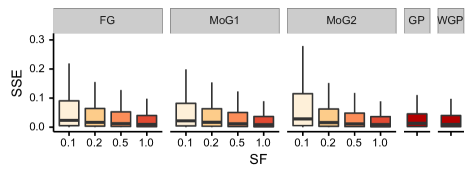
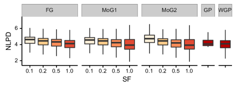
Figure 13: The distributions of sse and nlpd for a warped Gaussian process likelihood model on the creep dataset. Three approximate posteriors in savigp are used: fg (full Gaussian), mog1 (diagonal Gaussian), and mog2 (mixture of two diagonal Gaussians), along with various sparsity factors ($\text{SF}=M/N$). The smaller the sf the sparser the model, with $\text{SF}=1$ corresponding to the original model without sparsity. wgp corresponds to the performance of the exact inference method for warped Gaussian process models (Snelson et al., 2003), and gp is the performance of the exact inference on a univariate Gaussian likelihood model.

K.2 Medium-scale Experiments — Binary Classification

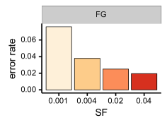
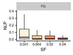
Figure 14: Error rates and nlp for binary classification on the mnist-b dataset. We used a full Gaussian (fg) posterior approximation across various sparsity factors ($\text{SF}=M/N$). The smaller the SF the sparser the model.

We see in Figure 14 that the performance improves significantly with denser models, i.e. when we use a larger number of inducing variables. Overall, our model achieves an accuracy of $98.1\%$ and a mean nlp of $0.062$ on mnist-b with a sparsity factor of $0.04$. This is slightly better than the performance obtained by Hensman et al. (2015), who report an accuracy of $97.8\%$ and nlp of $0.069$, although they used a smaller number of inducing variables. As we have seen in §9.5, our model also achieves similar performance when using the same sparsity factor as that used by Hensman et al. (2015) when the inducing inputs (i.e. the locations of the inducing variables) are learned.

K.3 Medium-scale Experiments — Gaussian Process Regression Networks

Figure 15: Mean sse and nlpd for multi-output regression on the sarcos dataset. We used a full Gaussian (fg) posterior approximation across various sparsity factors ($\text{SF}=M/N$). The smaller the SF the sparser the model.

Figure 15 shows the performance on the sarcos dataset. Compared to sarcos-2, learning all joints yields a slight increase in msse for joints $4$ and $7$, but also resulted in a significant decrease in nlpd. This shows that the transition from learning only $2$ joints to all $7$ joints (as in sarcos-2), while unhelpful for point estimates, led to a significantly better posterior density estimate. We also note that we had to make use of $10,000$ samples for this dataset to get stable results over different sparsity factors. This is a much larger number than the $100$ samples used in mnist. This is likely because the gprn likelihood model involves multiplication between latent processes, which increases the variance of sampling results by a squared factor, and therefore, it is reasonable to require more samples in this complex likelihood model.

K.4 Medium-scale Experiments — Inducing-input Learning

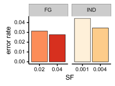
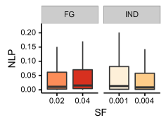
Figure 16: Comparison of error rate and nlp obtained by savigp without learning (fg) and with learning (ind) of inducing inputs for multi-class classification on the mnist dataset.

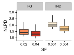
Figure 17: Comparison of mean sse and nlpd obtained by savigp without learning (fg) and with learning (ind) of inducing points for multi-output regression on the sarcos-2 dataset.

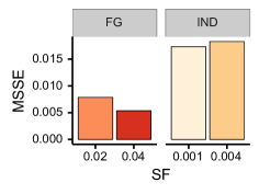
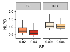
Figure 18: Comparison of mean sse and nlpd obtained by savigp without learning (fg) and with learning (ind) of inducing inputs for multi-output regression on the sarcos dataset.

Figure 16 shows the performance of the model under the two settings (with and without learning inducing inputs) on mnist. As with mnist-b, we see that learning the location of the inducing variables yields a large gain in performance. In fact, the sparser models with inducing point learning performed similarly to the denser models, despite the fact that the two models differed by an order of magnitude when it came to the number of inducing variables. Figures 17, 18 show the performance on sarcos and sarcos-2. We observe an improvement in performance from learning inducing inputs. However, the improvement is less significant than for mnist, which shows that different datasets have significantly different sensitivity to the location of the inducing variables.

Appendix L Notation

A summary of the notation used in this paper is shown in Table 4.

Table 4: Summary of notation used in the paper.

Symbol	Description
$\mathbf{v}$	Bold lower case denotes a vector
$\mathbf{C}$	Bold upper case denotes a matrix
$\left\lvert\mathbf{C}\right\rvert$	Determinant of matrix $\mathbf{C}$
$\mbox{ \rm tr }{\mathbf{C}}$	Trace of matrix $\mathbf{C}$
$D$	Input dimensionality
$N$	Number of training datapoints
$M$	Number of inducing variables per latent process
$P$	Number of outputs
$Q$	Number of latent functions
$K$	Number of mixture components in variational posterior
$S$	Number of samples in Monte Carlo estimates
$\mathbf{x}_{n}$	n$\mathrm{th}$ input datapoint
$\mathbf{X}$	$N\times D$ matrix of input data
$\mathbf{y}_{n}$	$P$-dimensional vector of outputs (label) for n$\mathrm{th}$ observation
$\mathbf{f}_{n\cdot}$	$Q$-dimensional vector of latent function values for n$\mathrm{th}$ observation
$\mathbf{f}_{\cdot j}$	$N$-dimensional vector of latent function values for $j\mathrm{th}$ process
$\mathbf{u}_{\cdot j}$	Inducing variables of latent process $j$
$\mathbf{u}$	Vector of all inducing variables
$\mathbf{Z}_{j}$	$M\times D$ Matrix of inducing inputs for latent process $j$
$\kappa_{j}(\mathbf{x},\mathbf{x}^{\prime})$	Covariance function of latent process $j$ evaluated at $\mathbf{x},\mathbf{x}^{\prime}$
$\mathbf{K}_{\mathbf{x}\mathbf{x}}^{j}$	$N\times N$ covariance matrix obtained by evaluating $\kappa_{j}(\mathbf{X},\mathbf{X})$
$\mathbf{K}_{\mathbf{z}\mathbf{z}}^{j}$	$M\times M$ covariance matrix obtained by evaluating $\kappa_{j}(\mathbf{Z}_{j},\mathbf{Z}_{j})$
$\mathbf{K}_{zz}$	Block-diagonal covariance with blocks $\mathbf{K}_{\mathbf{z}\mathbf{z}}^{j}$
$\mathbf{K}_{\mathbf{x}\mathbf{z}}^{j}$	$N\times M$ covariance between $\mathbf{X}$ and $\mathbf{Z}_{j}$
${\mathbf{k}_{\mathbf{z}n}^{j}}$	$M\times 1$ covariance vector between $\mathbf{Z}_{j}$ and $\mathbf{x}_{n}$
$q(\mathbf{u}|\boldsymbol{\lambda})$	Variational distribution over inducing variables
$q(\mathbf{f}|\boldsymbol{\lambda})$	Variational distribution over latent functions
$\mathbf{m}$	Posterior mean over inducing variables
$\mathbf{S}$	Posterior covariance over inducing variables
$\mathbf{b}$	Posterior mean over latent functions
$\mathbf{\Sigma}$	Posterior covariance over latent functions

References

- Al-Rfou et al. (2016) Rami Al-Rfou, Guillaume Alain, Amjad Almahairi, Christof Angermueller, and Dzmitry Bahdanau. Theano: A python framework for fast computation of mathematical expressions. arXiv preprint arXiv:1605.02688, 2016.
- Alvarez and Lawrence (2009) Mauricio Alvarez and Neil D Lawrence. Sparse convolved Gaussian processes for multi-output regression. In Neural Information Processing Systems, pages 57–64. 2009.
- Álvarez and Lawrence (2011) Mauricio A Álvarez and Neil D Lawrence. Computationally efficient convolved multiple output Gaussian processes. Journal of Machine Learning Research, 12(5):1459–1500, 2011.
- Álvarez et al. (2010) Mauricio A. Álvarez, David Luengo, Michalis K. Titsias, and Neil D. Lawrence. Efficient multioutput Gaussian processes through variational inducing kernels. In Artificial Intelligence and Statistics, 2010.
- Bache and Lichman (2013) K. Bache and M. Lichman. UCI machine learning repository, 2013. URL http://archive.ics.uci.edu/ml.
- Baydin et al. (2015) Atilim Gunes Baydin, Barak A Pearlmutter, Alexey Andreyevich Radul, and Jeffrey Mark Siskind. Automatic differentiation in machine learning: a survey. arXiv preprint arXiv:1502.05767, 2015.
- Bishop et al. (1998) Christopher M. Bishop, Neil D. Lawrence, Tommi Jaakkola, and Michael I. Jordan. Approximating posterior distributions in belief networks using mixtures. In M. I. Jordan, M. J. Kearns, and S. A. Solla, editors, Neural Information Processing Systems, pages 416–422. MIT Press, 1998.
- Bonilla et al. (2008) Edwin V. Bonilla, Kian Ming A. Chai, and Christopher K. I. Williams. Multi-task Gaussian process prediction. In Neural Information Processing Systems. 2008.
- Bonilla et al. (2010) Edwin V. Bonilla, Shengbo Guo, and Scott Sanner. Gaussian process preference elicitation. In Neural Information Processing Systems. 2010.
- Bonilla et al. (2016) Edwin V Bonilla, Daniel Steinberg, and Alistair Reid. Extended and unscented kitchen sinks. In International Conference on Machine Learning, 2016.
- Boyle and Frean (2005) Phillip Boyle and Marcus Frean. Dependent Gaussian processes. In Neural Information Processing Systems. 2005.
- Bui et al. (2017) Thang D Bui, Josiah Yan, and Richard E Turner. A unifying framework for Gaussian process pseudo-point approximations using power expectation propagation. The Journal of Machine Learning Research, 18(1):3649–3720, 2017.
- Casella and Robert (1996) George Casella and Christian P. Robert. Rao-Blackwellisation of sampling schemes. Biometrika, 1996.
- Challis and Barber (2013) Edward Challis and David Barber. Gaussian Kullback-Leibler approximate inference. Journal of Machine Learning Research, 14:2239–2286, 2013.
- Chu and Ghahramani (2005) Wei Chu and Zoubin Ghahramani. Gaussian processes for ordinal regression. Journal of Machine Learning Research, 6(Jul):1019–1041, 2005.
- Cole et al. (2000) D. Cole, C. Martin-Moran, A.G. Sheard, H.K.D.H. Bhadeshia, and D.J.C. MacKay. Modelling creep rupture strength of ferritic steel welds. Science and Technology of Welding & Joining, 5(2):81–89, 2000.
- Cressie (1993) Noel Cressie. Statistics for spatial data. John Wiley & Sons, 1993.
- Cutajar et al. (2017) Kurt Cutajar, Edwin V. Bonilla, Pietro Michiardi, and Maurizio Filippone. Random feature expansions for deep Gaussian processes. In International Conference on Machine Learning, volume 70, pages 884–893. PMLR, 06–11 Aug 2017.
- Damianou and Lawrence (2013) Andreas Damianou and Neil Lawrence. Deep Gaussian processes. In Artificial Intelligence and Statistics, 2013.
- Das et al. (2015) Sourish Das, Sasanka Roy, and Rajiv Sambasivan. Fast Gaussian process regression for big data. arXiv preprint arXiv:1509.05142, 2015.
- Deisenroth and Ng (2015) Marc Peter Deisenroth and Jun Wei Ng. Distributed Gaussian processes. In International Conference on Machine Learning, 2015.
- Dezfouli and Bonilla (2015) Amir Dezfouli and Edwin V. Bonilla. Scalable inference for Gaussian process models with black-box likelihoods. In Neural Information Processing Systems. 2015.
- Domingos et al. (2006) Pedro Domingos, Stanley Kok, Hoifung Poon, Matthew Richardson, and Parag Singla. Unifying logical and statistical AI. In AAAI Conference on Artificial Intelligence, 2006.
- Dong et al. (2017) Kun Dong, David Eriksson, Hannes Nickisch, David Bindel, and Andrew G Wilson. Scalable log determinants for Gaussian process kernel learning. In Neural Information Processing Systems, pages 6327–6337, 2017.
- Duane et al. (1987) Simon Duane, Anthony D. Kennedy, Brian J. Pendleton, and Duncan Roweth. Hybrid Monte Carlo. Physics letters B, 195(2):216–222, 1987.
- Gal and Turner (2015) Yarin Gal and Richard Turner. Improving the Gaussian process sparse spectrum approximation by representing uncertainty in frequency inputs. In International Conference on Machine Learning, pages 655–664, 2015.
- Gal et al. (2014) Yarin Gal, Mark van der Wilk, and Carl Rasmussen. Distributed variational inference in sparse Gaussian process regression and latent variable models. In Neural Information Processing Systems. 2014.
- Galliani et al. (2017) Pietro Galliani, Amir Dezfouli, Edwin V. Bonilla, and Novi Quadrianto. Gray-box inference for structured Gaussian process models. In Aarti Singh and Jerry Zhu, editors, Artificial Intelligence and Statistics, pages 353–361, Fort Lauderdale, FL, USA, Apr 2017. PMLR.
- Gelman and Rubin (1992) Andrew Gelman and Donald B Rubin. Inference from iterative simulation using multiple sequences. Statistical science, pages 457–472, 1992.
- Gershman et al. (2012) Samuel J. Gershman, Matthew D. Hoffman, and David M. Blei. Nonparametric variational inference. In International Conference on Machine Learning, 2012.
- Goodman et al. (2008) Noah D. Goodman, Vikash K. Mansinghka, Daniel M. Roy, Keith Bonawitz, and Joshua B. Tenenbaum. Church: A language for generative models. In Uncertainty in Artificial Intelligence, 2008.
- Henao and Winther (2012) Ricardo Henao and Ole Winther. Predictive active set selection methods for Gaussian processes. Neurocomputing, 80:10–18, 2012.
- Hensman et al. (2013) James Hensman, Nicolo Fusi, and Neil D Lawrence. Gaussian processes for big data. In Uncertainty in Artificial Intelligence, 2013.
- Hensman et al. (2015) James Hensman, Alexander Matthews, and Zoubin Ghahramani. Scalable variational Gaussian process classification. In Artificial Intelligence and Statistics, 2015.
- Hensman et al. (2017) James Hensman, Nicolas Durrande, and Arno Solin. Variational Fourier features for Gaussian processes. Journal of Machine Learning Research, 18:151:1–151:52, 2017.
- Hernández-Lobato and Hernández-Lobato (2016) Daniel Hernández-Lobato and José Miguel Hernández-Lobato. Scalable Gaussian process classification via expectation propagation. In Artificial Intelligence and Statistics, pages 168–176, 2016.
- Hinton and van Camp (1993) Geoffrey E. Hinton and Drew van Camp. Keeping the neural networks simple by minimizing the description length of the weights. In Sixth Annual Conference on Computational Learning Theory, pages 5–13. ACM, 1993.
- Hoang et al. (2015) Trong Nghia Hoang, Quang Minh Hoang, and Kian Hsiang Low. A unifying framework of anytime sparse Gaussian process regression models with stochastic variational inference for big data. In International Conference on Machine Learning, 2015.
- Hoffman and Gelman (2014) Matthew D. Hoffman and Andrew Gelman. The no-u-turn sampler: adaptively setting path lengths in Hamiltonian Monte Carlo. Journal of Machine Learning Research, 15(1):1593–1623, 2014.
- Huber et al. (2008) Marco F. Huber, Tim Bailey, Hugh Durrant-Whyte, and Uwe D. Hanebeck. On entropy approximation for Gaussian mixture random vectors. In IEEE International Conference on Multisensor Fusion and Integration for Intelligent Systems, 2008.
- Jarrett et al. (2009) Kevin Jarrett, Koray Kavukcuoglu, Marc’Aurelio Ranzato, and Yann Lecun. What is the best multi-stage architecture for object recognition? In International Conference on Computer Vision, 2009.
- Jarrett (1979) R.G. Jarrett. A note on the intervals between coal-mining disasters. Biometrika, 66(1):191–193, 1979.
- John and Hensman (2018) ST John and James Hensman. Large-scale Cox process inference using variational Fourier features. In International Conference on Machine Learning, 2018.
- Jordan et al. (1998) Michael I Jordan, Zoubin Ghahramani, Tommi S Jaakkola, and Lawrence K Saul. An introduction to variational methods for graphical models. Springer, 1998.
- Kersting et al. (2007) Kristian Kersting, Christian Plagemann, Patrick Pfaff, and Wolfram Burgard. Most likely heteroscedastic Gaussian process regression. In International Conference on Machine Learning, 2007.
- Khan et al. (2012) Mohammad E. Khan, Shakir Mohamed, Benjamin M. Marlin, and Kevin P. Murphy. A stick-breaking likelihood for categorical data analysis with latent Gaussian models. In Artificial Intelligence and Statistics, pages 610–618, 2012.
- Kingma and Welling (2014) Diederik P Kingma and Max Welling. Auto-encoding variational Bayes. In International Conference on Learning Representations, 2014.
- Krauth et al. (2017) Karl Krauth, Edwin V. Bonilla, Kurt Cutajar, and Maurizio Filippone. AutoGP: Exploring the capabilities and limitations of gaussian process models. In Uncertainty in Artificial Intelligence, 2017.
- Lappalainen and Miskin (2000) Harri Lappalainen and James W. Miskin. Ensemble Learning, pages 75–92. Springer London, London, 2000.
- Lauritzen (1981) Steffen L Lauritzen. Time series analysis in 1880: A discussion of contributions made by tn thiele. International Statistical Review, pages 319–331, 1981.
- Lawrence (2005) Neil Lawrence. Probabilistic non-linear principal component analysis with Gaussian process latent variable models. Journal of Machine Learning Research, 6:1783–1816, 2005.
- Lawrence et al. (2002) Neil D Lawrence, Matthias Seeger, and Ralf Herbrich. Fast sparse Gaussian process methods: The informative vector machine. In Neural Information Processing Systems, 2002.
- Lázaro-Gredilla et al. (2010) Miguel Lázaro-Gredilla, Joaquin Quiñonero-Candela, Carl Edward Rasmussen, and Aníbal R Figueiras-Vidal. Sparse spectrum Gaussian process regression. The Journal of Machine Learning Research, 99:1865–1881, 2010.
- Loosli et al. (2007) Gaëlle Loosli, Stéphane Canu, and Léon Bottou. Training invariant support vector machines using selective sampling. In Large Scale Kernel Machines, pages 301–320. MIT Press, Cambridge, MA., 2007.
- MacKay (1995) David J. C. MacKay. Developments in probabilistic modelling with neural networks — ensemble learning. In Bert Kappen and Stan Gielen, editors, Third Annual Symposium on Neural Networks, pages 191–198, London, 1995. Springer London.
- MacKay (2003) David J. C. MacKay. Information theory, inference and learning algorithms. Cambridge University Press, 2003.
- Matthews et al. (2016) Alexander G de G Matthews, James Hensman, Richard Turner, and Zoubin Ghahramani. On sparse variational methods and the Kullback-Leibler divergence between stochastic processes. Journal of Machine Learning Research, 51:231–239, 2016.
- Matthews et al. (2017) Alexander G. de G. Matthews, Mark van der Wilk, Tom Nickson, Keisuke. Fujii, Alexis Boukouvalas, Pablo Le’on-Villagr’a, Zoubin Ghahramani, and James Hensman. GPflow: A Gaussian process library using TensorFlow. Journal of Machine Learning Research, 18(40):1–6, apr 2017.
- Maz’ya and Schmidt (1996) Vladimir Maz’ya and Gunther Schmidt. On approximate approximations using Gaussian kernels. IMA Journal of Numerical Analysis, 16(1):13–29, 1996.
- Minka (2001) Thomas P Minka. Expectation propagation for approximate Bayesian inference. In Uncertainty in Artificial Intelligence, 2001.
- Møller et al. (1998) Jesper Møller, Anne Randi Syversveen, and Rasmus Plenge Waagepetersen. Log Gaussian Cox processes. Scandinavian journal of statistics, 25(3):451–482, 1998.
- Murray et al. (2010) Iain Murray, Ryan Prescott Adams, and David J.C. MacKay. Elliptical slice sampling. In Artificial Intelligence and Statistics, 2010.
- Neal (1993) Radford M. Neal. Probabilistic inference using Markov chain Monte Carlo methods. Technical report, Department of Computer Science, University of Toronto, 1993.
- Nguyen and Bonilla (2013) Trung V. Nguyen and Edwin Bonilla. Efficient variational inference for Gaussian process regression networks. In Artificial Intelligence and Statistics, pages 472–480, 2013.
- Nguyen and Bonilla (2014a) Trung V. Nguyen and Edwin V. Bonilla. Automated variational inference for Gaussian process models. In Neural Information Processing Systems. 2014a.
- Nguyen and Bonilla (2014b) Trung V. Nguyen and Edwin V. Bonilla. Collaborative multi-output Gaussian processes. In Uncertainty in Artificial Intelligence, 2014b.
- Nickisch and Rasmussen (2008) Hannes Nickisch and Carl Edward Rasmussen. Approximations for binary Gaussian process classification. Journal of Machine Learning Research, 9(10), 2008.
- O’Hagan and Kingman (1978) Anthony O’Hagan and JFC Kingman. Curve fitting and optimal design for prediction. Journal of the Royal Statistical Society. Series B (Methodological), pages 1–42, 1978.
- Opper and Archambeau (2009) Manfred Opper and Cédric Archambeau. The variational Gaussian approximation revisited. Neural Computation, 21(3):786–792, 2009.
- Paciorek and Schervish (2004) C Paciorek and M Schervish. Nonstationary covariance functions for Gaussian process regression. Neural Information Processing Systems, 2004.
- Quiñonero-Candela and Rasmussen (2005) Joaquin Quiñonero-Candela and Carl Edward Rasmussen. A unifying view of sparse approximate Gaussian process regression. Journal of Machine Learning Research, 6:1939–1959, 2005.
- Rahimi and Recht (2008) Ali Rahimi and Benjamin Recht. Random features for large-scale kernel machines. In Neural Information Processing Systems. 2008.
- Rahimi and Recht (2009) Ali Rahimi and Benjamin Recht. Weighted sums of random kitchen sinks: Replacing minimization with randomization in learning. In Neural Information Processing Systems. 2009.
- Ranganath et al. (2014) Rajesh Ranganath, Sean Gerrish, and David M. Blei. Black box variational inference. In Artificial Intelligence and Statistics, 2014.
- Ranzato et al. (2006) Marc’Aurelio Ranzato, Christopher Poultney, Sumit Chopra, and Yann Lecun. Efficient learning of sparse representations with an energy-based model. In Neural Information Processing Systems, 2006.
- Rasmussen and Williams (2006) Carl Edward Rasmussen and Christopher K. I. Williams. Gaussian processes for machine learning. The MIT Press, 2006.
- Reid et al. (2013) Alistair Reid, Simon O’Callaghan, Edwin V. Bonilla, Lachlan McCalman, Tim Rawling, and Fabio Ramos. Bayesian joint inversions for the exploration of Earth resources. In International Joint Conference on Artificial Intelligence, 2013.
- Rezende et al. (2014) Danilo J Rezende, Shakir Mohamed, and Daan Wierstra. Stochastic backpropagation and approximate inference in deep generative models. In International Conference on Machine Learning, 2014.
- Robbins and Monro (1951) Herbert Robbins and Sutton Monro. A stochastic approximation method. The annals of mathematical statistics, pages 400–407, 1951.
- Ross (2006) Sheldon M Ross. Simulation. Burlington, MA: Elsevier, 2006.
- Rue et al. (2009) Håvard Rue, Sara Martino, and Nicolas Chopin. Approximate Bayesian inference for latent Gaussian models by using integrated nested Laplace approximations. Journal of the royal statistical society: Series b (statistical methodology), 71(2):319–392, 2009.
- Salimbeni and Deisenroth (2017) Hugh Salimbeni and Marc Deisenroth. Doubly stochastic variational inference for deep Gaussian processes. In Advances in Neural Information Processing Systems, pages 4588–4599, 2017.
- Salimbeni et al. (2018) Hugh Salimbeni, Stefanos Eleftheriadis, and James Hensman. Natural gradients in practice: Non-conjugate variational inference in Gaussian process models. In Artificial Intelligence and Statistics, 2018.
- Sheth et al. (2015) Rishit Sheth, Yuyang Wang, and Roni Khardon. Sparse variational inference for generalized GP models. In International Conference on Machine Learning, 2015.
- Snelson and Ghahramani (2006) Ed Snelson and Zoubin Ghahramani. Sparse Gaussian processes using pseudo-inputs. In Neural Information Processing Systems, 2006.
- Snelson et al. (2003) Edward Snelson, Carl Edward Rasmussen, and Zoubin Ghahramani. Warped Gaussian processes. In Neural Information Processing Systems, 2003.
- Tarantola (2004) Albert Tarantola. Inverse Problem Theory and Methods for Model Parameter Estimation. Society for Industrial and Applied Mathematics, Philadelphia, PA, USA, 2004.
- Teh et al. (2005) Yee Whye Teh, Matthias Seeger, and Michael I. Jordan. Semiparametric latent factor models. In Artificial Intelligence and Statistics, 2005.
- Tipping (2001) Michael E Tipping. Sparse Bayesian learning and the relevance vector machine. Journal of machine learning research, 1(Jun):211–244, 2001.
- Titsias (2009) Michalis Titsias. Variational learning of inducing variables in sparse Gaussian processes. In Artificial Intelligence and Statistics, 2009.
- Vijayakumar and Schaal (2000) Sethu Vijayakumar and Stefan Schaal. Locally weighted projection regression: An O(n) algorithm for incremental real time learning in high dimensional space. In International Conference on Machine Learning, 2000.
- Williams and Barber (1998) Christopher K.I. Williams and David Barber. Bayesian classification with Gaussian processes. Pattern Analysis and Machine Intelligence, IEEE Transactions on, 20(12):1342–1351, 1998.
- Williams and Rasmussen (1996) Christopher KI Williams and Carl Edward Rasmussen. Gaussian processes for regression. In Neural Information Processing Systems, pages 514–520, 1996.
- Wilson et al. (2012) Andrew G. Wilson, David A. Knowles, and Zoubin Ghahramani. Gaussian process regression networks. In International Conference on Machine Learning, 2012.
- Wood et al. (2014) Frank Wood, Jan-Willem van de Meent, and Vikash Mansinghka. A new approach to probabilistic programming inference. In Artificial Intelligence and Statistics, pages 1024–1032, 2014.
- Yang et al. (2015) Zichao Yang, Andrew Gordon Wilson, Alexander J. Smola, and Le Song. À la carte — learning fast kernels. In Artificial Intelligence and Statistics, 2015.
- Yu and Chu (2008) Kai Yu and Wei Chu. Gaussian process models for link analysis and transfer learning. In Neural Information Processing Systems, 2008.
- Zeiler (2012) Matthew D Zeiler. ADADELTA: an adaptive learning rate method. arXiv preprint arXiv:1212.5701, 2012.