Circulant preconditioners for
discrete ill-posed Toeplitz systems

Abstract

Circulant preconditioners are commonly used to accelerate the rate of convergence of iterative methods when solving linear systems of equations with a Toeplitz matrix. Block extensions that can be applied when the system has a block Toeplitz matrix with Toeplitz blocks also have been developed. This paper is concerned with preconditioning of linear systems of equations with a symmetric block Toeplitz matrix with symmetric Toeplitz blocks that stem from the discretization of a linear ill-posed problem. The right-hand side of the linear systems represents available data and is assumed to be contaminated by error. These kinds of linear systems arise, e.g., in image deblurring problems. It is important that the preconditioner does not affect the invariant subspace associated with the smallest eigenvalues of the block Toeplitz matrix to avoid severe propagation of the error in the right-hand side. A perturbation result indicates how the dimension of the subspace associated with the smallest eigenvalues should be chosen and allows the determination of a suitable preconditioner when an estimate of the error in the right-hand side is available. This estimate also is used to decide how many iterations to carry out by a minimum residual iterative method. Applications to image restoration are presented.

Dedicated to Ken Hayami on the occasion of his 60th birthday.

AMS subject classifications. 65F10, 65F15, 65F30.

1 Introduction

Linear systems of equations with a matrix with a Toeplitz-type structure arise in many applications, such as in signal and image processing. Consider the computation of an approximate solution of the linear system of equations

$$T{\mbox{\boldmath{$x$}}}={\mbox{\boldmath{$b$}}},\qquad T\in{{\mathbb{R}}}^{n_{1}n_{2}\times n_{1}n_{2}},\qquad{\mbox{\boldmath{$x$}}},{\mbox{\boldmath{$b$}}}\in{{\mathbb{R}}}^{n_{1}n_{2}},$$ (1)

where $T$ is a symmetric BTTB matrix, i.e., $T$ is a symmetric block Toeplitz matrix with each block being an $n_{1}\times n_{1}$ symmetric Toeplitz matrix. The eigenvalues of $T$ are assumed to decay smoothly to zero in magnitude without a significant gap. In particular, $T$ may be singular. Linear systems of equations (1) with a matrix of this kind arise, for example, from the discretization of a linear ill-posed problem, such as a Fredholm integral equation of the first kind in two space-dimensions with a displacement kernel.

The right-hand side $b$ of (1) is assumed to be contaminated by an (unknown) error $e$. We will refer to this error as “noise”. It may stem from measurement or discretization errors. Let $\widehat{\mbox{\boldmath{$b$}}}$ denote the (unknown) error-free vector associated with $b$, i.e.,

$${\mbox{\boldmath{$b$}}}=\widehat{\mbox{\boldmath{$b$}}}+{\mbox{\boldmath{$e$}}}.$$ (2)

The (unknown) linear system of equations with error-free right-hand side,

$$T{\mbox{\boldmath{$x$}}}=\widehat{\mbox{\boldmath{$b$}}},$$ (3)

is assumed to be consistent; however, we do not require the available system (1) to be consistent.

We will assume that a fairly sharp bound for the norm of $e$ is known, i.e.,

$$\|\mbox{\boldmath{$e$}}\|\leq\varepsilon.$$ (4)

Here and throughout this paper $\|\cdot\|$ denotes the Euclidean vector norm or the spectral matrix norm. This bound will help us determine a suitable number of iterations to carry out with a minimal residual iterative method and to construct a preconditioner for the solution of (1).

Let $T^{\dagger}$ denote the Moore–Penrose pseudoinverse of $T$. We are interested in computing an approximation of the solution $\widehat{\mbox{\boldmath{$x$}}}=T^{\dagger}\widehat{\mbox{\boldmath{$b$}}}$ of minimal Euclidean norm of the unavailable error-free linear system (3). Note that the solution of (1),

$$\mbox{\boldmath{$x$}}=T^{\dagger}{\mbox{\boldmath{$b$}}}=T^{\dagger}(\widehat{\mbox{\boldmath{$b$}}}+{\mbox{\boldmath{$e$}}})=\widehat{\mbox{\boldmath{$x$}}}+T^{\dagger}{\mbox{\boldmath{$e$}}},$$

typically is dominated by the propagated error $T^{\dagger}{\mbox{\boldmath{$e$}}}$ and, therefore, is useless. Therefore all solution methods for (1) seek to determine a suitable approximate solution that is not severely contaminated by propagated error. The computed approximate solution is the exact solution of an appropriately chosen nearby problem, whose solution is less sensitive to the error $e$ in $b$ than the solution of (1). The replacement of the given problem (1) by a nearby problem is commonly referred to as regularization. Among the most popular regularization methods is Tikhonov regularization, which replaces (1) by a penalized least-squares problem, and truncated iteration, which is based on solving (1) by an iterative method and terminating the iterations suitably early, see, e.g., [7, 10, 13, 17] for discussions on these regularization methods. In this paper we regularize by truncated iteration, and by choosing a suitable preconditioner.

The evaluation of matrix-vector products with a BTTB matrix of order $n_{1}n_{2}$ can be carried out in only ${\mathcal{O}}(n_{1}n_{2}\log_{2}(n_{1}n_{2}))$ arithmetic floating point operations (flops) by using the fast Fourier transform (FFT); see, e.g., [1, 12]. This makes it attractive to solve (1) by an iterative method. We will use a preconditioner to increase the rate of convergence of the iterative method. BTTB matrices are commonly preconditioned by block circulant with circulant block (BCCB) matrices; see [1, 3, 12, 19, 20] for discussions, illustrations, and further references. The use of BCCB preconditioners for BTTB matrices is attractive both due to the spectral properties of the preconditioned matrix and because of the possibility to evaluate a matrix-vector product with a preconditioned matrix of order $n_{1}n_{2}$ in only ${\mathcal{O}}(n_{1}n_{2}\log_{2}(n_{1}n_{2}))$ flops with the aid of the FFT. A MATLAB software package for fast matrix-vector product evaluation is provided by Redivo–Zaglia and Rodriguez [16].

When preconditioning a BTTB matrix $T$ that stems from the discretization of a linear ill-posed problem, it is desirable that an invariant subspace associated with the eigenvalues of $T$ of smallest magnitude is not affected by preconditioning to avoid severe propagation of the error $e$ in the right-hand side $b$ of (1) into the computed iterates. This is due to the fact that the eigenvectors associated with these eigenvalues are highly oscillatory (have many sign changes) and model noise rather than the desired solution $\widehat{\mbox{\boldmath{$x$}}}$. Typically, we do not want these eigenvectors to be part of our computed approximation of $\widehat{\mbox{\boldmath{$x$}}}$. A nice introduction to BCCB preconditioners for the solution of discretized linear ill-posed problems with a Toeplitz-type matrix is presented by Hanke et al. [9].

The number of iterations have to be few enough to avoid severe propagation of the error $e$ in $b$ into the computed approximation of $\widehat{\mbox{\boldmath{$x$}}}$. The availability of the bound (4) and the consistency of (3) allow us to apply the discrepancy principle to determine a suitable number of iterations as well as to define the dimension of the invariant subspace that should not be affected by the preconditioner. Roughly, the larger the error in $b$, the larger should the dimension of the subspace that is not (or only minimally) affected by preconditioning be chosen.

Various other approaches to define BCCB preconditioners for the iterative solution of discretized linear ill-posed problems (1) with an error-contaminated right-hand side are described in the literature. For instance, Hanke and Nagy [8] apply the L-curve criterion to determine a subspace that should not be affected by the preconditioner. The L-curve criterion implicitly estimates the norm of the error in $b$. This criterion is able to estimate the norm of the error fairly accurately in some situations, but it is not a reliable error estimator; see [13, 17] for discussions and illustrations. We therefore are interested in developing an approach for constructing BCCB preconditioners that is not based on the L-curve criterion. Hanke et al. [9] apply a discrete Picard condition to determine the dimension of the subspace that the BCCB preconditioner should leave invariant. This approach typically works quite well in an interactive computing environment that allows the determination of whether the discrete Picard condition holds by visual inspection, however, it is not straightforward to automatize. Di Benedetto et al. [4] propose the application of a so-called superoptimal BCCB preconditioner and do not explicitly choose the dimension of the subspace that should be unaffected by the preconditioner. This approach works well for some image restoration problems, but not for others; see the discussion in [4].

Preconditioning is most useful when the error $e$ in $b$ is of small relative norm, because then many steps of an iterative method may be required to determine an accurate approximation of $\widehat{\mbox{\boldmath{$x$}}}$. When the error $e$ is large, only few steps can be carried out before the propagated error destroys the computed solution. Preconditioning then does not reduce the computational effort by much.

In this paper, we will use the bound (4) to determine both the BCCB preconditioner and the number of iterations to be carried out. A perturbation bound guides our choice of preconditioner. This is described in Section 2. A few computed examples are presented in Section 3 and concluding remarks can be found in Section 4.

2 Preconditioned iterative regularization

We discuss the construction of the preconditioner, the stopping criterion for the iterative method, and outline the minimal residual iterative methods used.

2.1 The BCCB preconditioner

Let for the moment $T\in{\mathbb{R}}^{n\times n}$ be a symmetric positive definite Toeplitz matrix and let $C\in{\mathbb{R}}^{n\times n}$ be the closest circulant matrix to $T$ in the Frobenius norm. T. Chan [2] proposed the use of $C$ as a preconditioner for $T$; see also [1, 12]. The eigenvalues of $C$ are given by the discrete Fourier transform of the first column of $C$; their computation with the FFT requires only ${\mathcal{O}}(n\log_{2}(n))$ flops. Since we would like the preconditioner not to affect the invariant subspace of $T$ associated with the smallest eigenvalues, we set the $n-p$ eigenvalues of smallest magnitude of $C$ to unity for some suitable $0\leq p\leq n$, analogously as in [8, 9]. We refer to this preconditioner as $C_{p}$. Subsection 2.3 describes how to determine $p$ using the error bound (4).

The linear systems (1) of interest to us have a BTTB matrix $T$, i.e., $T$ is the Kronecker product of two Toeplitz matrices

$$T=T_{1}\otimes T_{2},\qquad T_{1}\in{\mathbb{R}}^{n_{1}\times n_{1}},\qquad T_{2}\in{\mathbb{R}}^{n_{2}\times n_{2}}.$$ (5)

We will determine a preconditioner that is the Kronecker product of two circulant matrices

$$C=C_{p_{1}}\otimes C_{p_{2}},\qquad C_{p_{1}}\in{\mathbb{R}}^{n_{1}\times n_{1}},\qquad C_{p_{2}}\in{\mathbb{R}}^{n_{2}\times n_{2}},$$ (6)

where $C_{p_{j}}$ is defined by first determining the closest circulant $C_{j}$ to $T_{j}$ in the Frobenius norm and then setting its $n_{j}-p_{j}$ eigenvalues of smallest magnitude to one for $j=1,2$. In this way our preconditioner $C$ does not affect the invariant subspace of $T$ associated with the eigenvalues of smallest magnitude. The eigenvectors of this subspace are highly oscillatory and primarily model noise and not the desired solution $\widehat{\mbox{\boldmath{$x$}}}$. This construction of $C$ requires only ${\mathcal{O}}(n_{1}n_{2}(\log_{2}(n_{1})+\log_{2}(n_{2}))$ flops. We refer to the BCCB preconditioner so determined as $C_{p_{1},p_{2}}$. The determination of this preconditioner is somewhat faster than of the BCCB preconditioner described in [9], because the latter requires that all its $n_{1}n_{2}$ eigenvalues be formed.

2.2 Stopping criterion

Once the BCCB preconditioner $C_{p_{1},p_{2}}$ has been defined, we compute an approximate solution ${\mbox{\boldmath{$y$}}}_{k}$ of the preconditioned linear system of equations,

$$TC_{p_{1},p_{2}}^{-1}{\mbox{\boldmath{$y$}}}={\mbox{\boldmath{$b$}}},$$ (7)

using one of the minimal residual iterative methods described in Subsection 2.5. As for the initial approximation of $\widehat{\mbox{\boldmath{$x$}}}$, define the BCCB matrix $\widetilde{C}_{p_{1},p_{2}}=\widetilde{C}_{p_{1}}\otimes\widetilde{C}_{p_{2}}$, where $\widetilde{C}_{p_{j}}$ is obtained from $C_{j}$ by setting the $n_{j}-p_{j}$ eigenvalues of smallest magnitude to zero, for $j=1,2$, and define

$${\mbox{\boldmath{$x$}}}_{0}=\widetilde{C}_{p_{1},p_{2}}^{{\dagger}}{\mbox{\boldmath{$b$}}},\qquad{\mbox{\boldmath{$r$}}}_{0}={\mbox{\boldmath{$b$}}}-T{\mbox{\boldmath{$x$}}}_{0}.$$ (8)

The initial iterate then is chosen to be ${\mbox{\boldmath{$y$}}}_{0}=C_{p_{1},p_{2}}{\mbox{\boldmath{$x$}}_{0}}$.

Let ${\mbox{\boldmath{$y$}}}_{1},{\mbox{\boldmath{$y$}}_{2}},\ldots~{}$ denote the computed iterates. The number of iterations to be carried out is determined with the aid of the discrepancy principle. This stopping criterion prescribes that the iterations be terminated as soon as an iterate $\mbox{\boldmath{$y$}}_{k}$ satisfies

$$\|TC_{p_{1},p_{2}}^{-1}\mbox{\boldmath{$y$}}_{k}-\mbox{\boldmath{$r$}}_{0}\|\leq\gamma\varepsilon,$$ (9)

where $\gamma\geq 1$ is a user-specified parameter independent of $\varepsilon$. Typically, $\gamma$ is chosen close to unity when $\varepsilon$ is known to be a fairly sharp upper bound for $\|\mbox{\boldmath{$e$}}\|$; cf. (4). We obtain the approximation

$${\mbox{\boldmath{$x$}}}_{k}={\mbox{\boldmath{$x$}}_{0}}+C_{p_{1},p_{2}}^{-1}{\mbox{\boldmath{$y$}}}_{k}$$

of the desired vector $\widehat{\mbox{\boldmath{$x$}}}$.

2.3 Construction of the preconditioner

Let for the moment $T\in{\mathbb{R}}^{n\times n}$ be a Toeplitz matrix and let $C\in{\mathbb{R}}^{n\times n}$ be the closest circulant in the Frobenius norm. Order the eigenvalues of $C$ according to

$$|\lambda_{1}|\geq|\lambda_{2}|\geq\dots\geq|\lambda_{n}|\geq 0.$$

Assume that a bound (4) is known. Let $p$ be the number of eigenvalues of largest magnitude of $C$ that are not set to unity. We choose $p=\lfloor\frac{3}{4}q\rfloor$, where $q$ is the solution of the minimization problem

$$\min_{1\leq q<n}\frac{1}{|\lambda_{q}|}\left(\frac{|\lambda_{q+1}|}{|\lambda_{1}|}+\eta\right).$$ (10)

Here $\lfloor\alpha\rfloor$ denotes the largest integer smaller than or equal to $\alpha\geq 0$ and $\eta=\varepsilon/\|{\mbox{\boldmath{$b$}}}\|$. This choice of $p$ is suggested by the following perturbation result.

Proposition 1.

Given a rank-$q$ matrix $A\in{{\mathbb{C}}}^{n\times n}$, $q\leq n$, a vector $\mbox{\boldmath{$\beta$}}\neq\mbox{\boldmath{$0$}}$ in the range of $A$, and $\xi$ such that ${\mbox{\boldmath{$\xi$}}}=A^{{\dagger}}{\mbox{\boldmath{$\beta$}}}$. Let $\Delta A$, $\Delta\beta$, and $\Delta\xi$ satisfy

$$(A+\Delta A)({\mbox{\boldmath{$\xi$}}}+{\mbox{\boldmath{$\Delta\xi$}}})={\mbox{\boldmath{$\beta$}}}+{\mbox{\boldmath{$\Delta\beta$}}}.$$

Then

$$\frac{\|{\mbox{\boldmath{$\Delta\xi$}}}\|}{\|{\mbox{\boldmath{$\xi$}}}\|}\leq\nu(A,A+\Delta A)\,\kappa(A)\left(\frac{\|\Delta A\|}{\|A\|}+\frac{\|{\mbox{\boldmath{$\Delta\beta$}}}\|}{\|{\mbox{\boldmath{$\beta$}}}\|}\right),$$ (11)

where $\kappa(M)=\|M\|\|M^{{\dagger}}\|$ is the condition number of the matrix $M$, and $\nu(M,N)$ denotes the ratio between the smallest singular values of the matrices $M$ and $N$.

Proof.

From $A{\mbox{\boldmath{$\xi$}}}={\mbox{\boldmath{$\beta$}}}$ and $(A+\Delta A){\mbox{\boldmath{$\Delta\xi$}}}=-\Delta A{\mbox{\boldmath{$\xi$}}}+{\mbox{\boldmath{$\Delta\beta$}}}$, one has

$${\mbox{\boldmath{$\Delta\xi$}}}=(A+\Delta A)^{{\dagger}}\left(-\Delta A{\mbox{\boldmath{$\xi$}}}+{\mbox{\boldmath{$\Delta\beta$}}}\right).$$

Taking norms on both sides, one gets

$$\|{\mbox{\boldmath{$\Delta\xi$}}}\|\leq\|(A+\Delta A)^{{\dagger}}\|\left(\|\Delta A\|\|{\mbox{\boldmath{$\xi$}}}\|+\|{\mbox{\boldmath{$\Delta\beta$}}}\|\right).$$

Hence,

$$\|{\mbox{\boldmath{$\Delta\xi$}}}\|\leq\nu(A,A+\Delta A)\,\kappa(A)\left(\frac{\|\Delta A\|\|{\mbox{\boldmath{$\xi$}}}\|}{\|A\|}+\frac{\|\mbox{\boldmath{$\Delta\beta$}}\|}{\|A\|}\right).$$

Finally, dividing by $\|{\mbox{\boldmath{$\xi$}}}\|$ and exploiting the inequality $\|{\mbox{\boldmath{$\beta$}}}\|\leq\|A\|\|\mbox{\boldmath{$\xi$}}\|$ yield (11). ∎

Let $\widetilde{C}_{q}$ be the circulant obtained by setting the $n-q$ eigenvalues of smallest magnitude of $C$ to zero. In this context, one replaces $A$ by $\widetilde{C}_{q}$ and $\beta$ by $b$ in Proposition 1. Now, letting $\Delta A=T-\widetilde{C}_{q}$ and ${\mbox{\boldmath{$\Delta\beta$}}}=-\mbox{\boldmath{$e$}}$, we obtain by (2) that ${\mbox{\boldmath{$\Delta\xi$}}}=\hat{\mbox{\boldmath{$x$}}}-\widetilde{C}_{q}^{{\dagger}}{\mbox{\boldmath{$b$}}}$ satisfies the hypothesis of Proposition 1. Inequality (11) reads

$$\frac{\|\hat{\mbox{\boldmath{$x$}}}-\widetilde{C}_{q}^{{\dagger}}{\mbox{\boldmath{$b$}}}\|}{\|{\mbox{\boldmath{$x$}}_{0}}\|} \leq \nu(\widetilde{C}_{q},T)\,\kappa(\widetilde{C}_{q})\left(\frac{\|T-\widetilde{C}_{q}\|}{\|\widetilde{C}_{q}\|}+\frac{\|\mbox{\boldmath{$e$}}\|}{\|\mbox{\boldmath{$b$}}\|}\right)$$

$$\leq \nu(\widetilde{C}_{q},T)\,\frac{|\lambda_{1}|}{|\lambda_{q}|}\left(\frac{\|T-\widetilde{C}_{q}\|}{|\lambda_{1}|}+\eta\right)\sim\frac{|\lambda_{1}|}{|\lambda_{q}|}\left(\frac{|\lambda_{q+1}|}{|\lambda_{1}|}+\eta\right).$$

In the final estimate, we assume that the eigenvalues of $T$ of smallest magnitude are close to $|\lambda_{q}|$, so that $\nu(\widetilde{C}_{q},T)\sim 1$ and $\|T-\widetilde{C}_{q}\|\sim\|C-\widetilde{C}_{q}\|$. This discussion suggests the choice $p=q$, where $q$ is determined by (10). However, since we do not know whether the eigenvalues of $T$ of smallest magnitude are close to $|\lambda_{q}|$, we will choose $p=\lfloor 3q/4\rfloor$ to secure that we do not “over-precondition” and thereby obtain a large propagated error in the computed approximation of $\widehat{\mbox{\boldmath{$x$}}}$. We remark that a “standard” circulant preconditioner $\widetilde{C}_{n}$ generally over-preconditions and gives a large propagated error in the computed solution.

We turn to BTTB matrices and first consider the matrix $T\otimes T$. Let $C$ be the closest circulant to $T$ in the Frobenius norm. Then $C\otimes C$ is the closest BCCB matrix to $T\otimes T$ in the Frobenius norm. Let $q$ to be the solution of the minimization problem

$$\min_{1\leq q<n}\frac{1}{|\lambda_{q}|^{2}}\left(\frac{|\lambda_{q+1}|^{2}}{|\lambda_{1}|^{2}}+\eta\right),$$ (12)

where $\eta=\varepsilon/\|{\mbox{\boldmath{$b$}}}\|$. The choice $p=q$ is suggested by Proposition 1, where one replaces $A$ by $\widetilde{C}_{p,p}$, the BCCB matrix obtained setting the $n-p$ eigenvalues of smallest magnitude of each circulant matrix $C$ to zero, and replaces $\beta$ by $b$, so that the vector $\xi$ in Proposition 1 is given by ${\mbox{\boldmath{$x$}}_{0}}$ in (8) with $p_{1}=p_{2}=q$. In the computed examples, we will let $p_{1}=p_{2}=\lfloor 3q/4\rfloor$ to avoid to over-precondition.

Finally, consider BTTB matrices of the form (5). To determine a BCCB preconditioner of the kind (6), we sort the eigenvalues of the circulant matrices $C_{j}$, $j=1,2$, according to

$$|\lambda_{1}^{(j)}|\geq|\lambda_{2}^{(j)}|\geq\dots\geq|\lambda_{n_{j}}^{(j)}|\geq 0,$$

and let $p_{j}$ be the number of eigenvalues of largest magnitude of $C_{j}$ that are not set to unity. Let the index pair $\{q_{1},q_{2}\}$ solve the minimization problem

$$\min_{\begin{subarray}{c}1\leq q_{1}<n_{1}\\ 1\leq q_{2}<n_{2}\end{subarray}}\frac{1}{|\lambda^{(1)}_{q_{1}}||\lambda^{(2)}_{q_{2}}|}\left(\frac{|\lambda^{(1)}_{q_{1}+1}||\lambda^{(2)}_{q_{2}+1}|}{|\lambda^{(1)}_{1}||\lambda^{(2)}_{1}|}+\eta\right),$$ (13)

where $\eta=\varepsilon/\|{\mbox{\boldmath{$b$}}}\|$. Similarly as above, we let $p_{j}=\lfloor 3q_{j}/4\rfloor$ for $j=1,2$.

2.4 Construction of the preconditioned system

The preconditioned matrix $TC_{p_{1},p_{2}}^{-1}$, where $T$ and $C_{p_{1},p_{2}}$ are given by (5) and (6), respectively, is constructed as follows:

Compute for $j=1,2$:

1. The closest circulant $C_{j}$ to $T_{j}$ in the Frobenius norm.

2. The FFT of the first column of the matrix $C_{j}$. This gives the eigenvalues $\lambda^{(j)}_{1},\lambda^{(j)}_{2},\ldots,\lambda^{(j)}_{n_{j}}$ of $C_{j}$. The eigenvectors are the columns of the Fourier matrix. Permute the columns of the Fourier matrix so that the eigenvalues are ordered according to decreasing magnitude,

   $$|\lambda^{(j)}_{1}|\geq|\lambda^{(j)}_{2}|\geq\ldots\geq|\lambda^{(j)}_{n_{j}}|$$

   and denote the permuted Fourier matrix by $U_{j}$. The columns of $U_{j}$ generally become more oscillatory with increasing column number.

3. The truncation index $p_{j}$, $1\leq p_{j}\leq n_{j}$, by using (13). This defines the diagonal matrices

   $$\Lambda_{p_{j}} = {\rm diag}[\lambda^{(j)}_{1},\lambda^{(j)}_{2},\ldots,\lambda^{(j)}_{p_{j}},1,\ldots,1],$$

   $$\widetilde{\Lambda}_{p_{j}} = {\rm diag}[\lambda^{(j)}_{1},\lambda^{(j)}_{2},\ldots,\lambda^{(j)}_{p_{j}},0,\ldots,0].$$

   Neither the matrices $U_{j}$ nor $\Lambda_{p_{j}}$ and $\widetilde{\Lambda}_{p_{j}}$ have to be explicitly formed.

We are now in a position to define the preconditioner and related matrices, but hasten to point out that these matrices do not have to be explicitly formed. Introduce

$$\begin{array}[]{rclcrclcrcl}C_{p_{j}}&=&U_{j}\Lambda_{p_{j}}U_{j}^{*},&{}{}\hfil&C_{p_{j}}^{-1}&=&U_{j}\Lambda_{p_{j}}^{-1}U_{j}^{*},&{}{}\hfil&\widetilde{C}_{p_{j}}^{{\dagger}}&=&U_{j}\widetilde{\Lambda}_{p_{j}}^{{\dagger}}U_{j}^{*},\\ C_{p_{1},p_{2}}&=&C_{p_{1}}\otimes C_{p_{2}},&{}{}\hfil&C_{p_{1},p_{2}}^{-1}&=&C_{p_{1}}^{-1}\otimes C_{p_{2}}^{-1},&{}{}\hfil&\widetilde{C}_{p_{1},p_{2}}^{{\dagger}}&=&\widetilde{C}_{p_{1}}^{{\dagger}}\otimes\widetilde{C}_{p_{2}}^{{\dagger}},\end{array}$$

where the superscript ^∗ denotes transposition and complex conjugation. We compute the initial approximate solution ${\mbox{\boldmath{$x$}}_{0}}=\widetilde{C}_{p_{1},p_{2}}^{{\dagger}}{\mbox{\boldmath{$b$}}}$ in (8) without explicitly forming the matrix $\widetilde{C}_{p_{1},p_{2}}^{{\dagger}}$. Indeed, the spectral factorization

$$C_{p_{1},p_{2}}=C_{p_{1}}\otimes C_{p_{2}}=(U_{1}\otimes U_{2})(\Lambda_{p_{1}}\otimes\Lambda_{p_{2}})(U_{1}\otimes U_{2})^{*},$$

can be applied to evaluate $C_{p_{1},p_{2}}\mbox{\boldmath{$y$}}$ for any $\mbox{\boldmath{$y$}}\in{{\mathbb{R}}}^{n_{1}n_{2}}$ in ${\mathcal{O}}(n_{1}n_{2}\log_{2}(n_{1}n_{2}))$ flops with the FFT, and the same holds for matrix-vector products with the matrices $C_{p_{1},p_{2}}^{-1}$ and $\widetilde{C}_{p_{1},p_{2}}^{{\dagger}}$.

Krylov subspace methods for the iterative solution of (7) require matrix-vector product evaluations with the preconditioned matrix $TC^{-1}_{p_{1},p_{2}}$. It is well known that these matrix-vector product evaluations can be carried out quickly with the aid of the FFT. We outline for completeness the evaluation of matrix-vector products with the matrix $TC_{p}^{-1}$ in the simplified situation when $T\in{\mathbb{R}}^{n\times n}$ is a Toeplitz matrix and $C_{p}$ is a circulant. We express $T$ as a sum of a circulant $C_{0}$ and a skew-circulant $C_{\pi}$. This splitting and the spectral factorizations

$$C_{0}=U\Lambda_{0}U^{*},\quad C_{\pi}=U_{\pi}\Lambda_{\pi}U_{\pi}^{*},$$

where $U_{\pi}=\mathop{\operator@font diag}\nolimits\{1,e^{i\pi/n},\dots,e^{(n-1)i\pi/n}\}U$, yield that

$$TC_{p}^{-1}=(C_{0}+C_{\pi})C_{p}^{-1}=(U\Lambda_{0}U^{*}+U_{\pi}\Lambda_{\pi}U_{\pi}^{*})U\Lambda_{p}^{-1}U^{*}.$$

The preconditioned linear system of equations $TC_{p}^{-1}\mbox{\boldmath{$x$}}=\mbox{\boldmath{$b$}}$ with $\mbox{\boldmath{$b$}}\in{\mathbb{R}}^{n}$ can be expressed in the form

$$(\Lambda_{0}+U^{*}U_{\pi}\Lambda_{\pi}U_{\pi}^{*}U)\Lambda_{p}^{-1}\mbox{\boldmath{$y$}}=U^{*}\mbox{\boldmath{$b$}},\qquad\mbox{\boldmath{$x$}}=U\mbox{\boldmath{$y$}},$$

which is used in the computations. Each iteration requires the evaluation of the FFT of four $n$-vectors. The computation of these FFTs is the dominating computational work. We remark that the dominating computational effort to evaluate a matrix-vector product with the matrix $T$, which is required when solving the unpreconditioned system $T\mbox{\boldmath{$x$}}=\mbox{\boldmath{$b$}}$ by a Krylov subspace method, also is the computation of the FFT of four $n$-vectors. Therefore, the number of iterations required by the iterative method is the proper measure of the computational effort both for preconditioned and unpreconditioned linear systems of equations. The situation is analogous when $T$ is the tensor product of two Toeplitz matrices. We omit the details.

2.5 Range restricted GMRES and MINRES methods

GMRES is a popular iterative method for the solution of large linear systems of equations $A{\mbox{\boldmath{$x$}}}={\mbox{\boldmath{$b$}}}$ with a square nonsingular nonsymmetric matrix $A$ that arise from the discretization of well-posed problems, such as Dirichlet boundary value problems for elliptic partial differential equations; see, e.g., Saad [18]. The $k$th iterate determined by this method solves the minimization problem

$$\min_{\mbox{\boldmath{${\scriptstyle x}$}}\in{\mathcal{K}}_{k}(A,{\mbox{\boldmath{${\scriptstyle r}$}}}_{0})}\|A\mbox{\boldmath{$x$}}-\mbox{\boldmath{$r$}}_{0}\|,$$

where $\mbox{\boldmath{$x$}}_{0}$ is an initial approximate solution, ${\mbox{\boldmath{$r$}}}_{0}={\mbox{\boldmath{$b$}}}-A{\mbox{\boldmath{$x$}}}_{0}$, and

$${\mathcal{K}}_{k}(A,{\mbox{\boldmath{$r$}}}_{0})=\mbox{span}\{\mbox{\boldmath{$r$}}_{0},A\mbox{\boldmath{$r$}}_{0},\ldots,A^{k-1}{\mbox{\boldmath{$r$}}}_{0}\}$$

is a Krylov subspace.

It has been observed that a modification of GMRES, which we refer to as the range restricted GMRES method (RRGMRES), often yields a more accurate approximation of the desired solution $\widehat{\mbox{\boldmath{$x$}}}$ than (standard) GMRES when $A$ stems from the discretization of a linear ill-posed problem and the right-hand side $b$ is contaminated by error; see [6, 14]. The RRGMRES method determines iterates in shifted Krylov subspaces ${\mathcal{K}}_{k}(A,A^{\ell}{\mbox{\boldmath{$r$}}}_{0})$, where $\ell\geq 1$ is a small integer. We propose that an RRGMRES method be used for the solution of the preconditioned problem

$$TC_{p_{1},p_{2}}^{-1}\mbox{\boldmath{$y$}}=\mbox{\boldmath{$r$}}_{0}.$$

When $T$ and $C_{p_{1},p_{2}}$ are symmetric positive definite, RRGMRES can be simplified to a range restricted MINRES method that only requires simultaneous storage of a few $n$-vectors, the number of which is bounded independently of the number of iterations; see [5] for details.

3 Computed examples

The calculations of this section were carried out in MATLAB with machine epsilon about $2.2\cdot 10^{-16}$. For all the examples, we chose $\gamma=1$ in (9).

Example 1. This is an image deblurring test problem from the MATLAB package Regularization Tools [11]. The original image and the symmetric BTTB matrix are those defined by the MATLAB function blur.m. We choose the dimensions $n_{1}=n_{2}=64$, half-bandwidth for each Toeplitz block specified by the parameter $band=10$ and width of the Gaussian point spread specified by the parameter $sigma=\sqrt{5}$.

% relative data error	$p$	steps $k$	$\|\mbox{\boldmath{$x$}}_{k}-\widehat{\mbox{\boldmath{$x$}}}\|/\|\widehat{\mbox{\boldmath{$x$}}}\|$
$0.10$	$14$	$18$	$0.3404$
$0.10$	$-$	$33$	$0.3361$
$0.05$	$16$	$22$	$0.3308$
$0.05$	$-$	$45$	$0.3275$
$0.01$	$17$	$42$	$0.3094$
$0.01$	$-$	$89$	$0.3072$

Table 1: Example 1: blur. A hyphen signifies that no preconditioner is used.

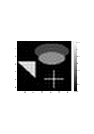
(a)	(b)

Fig. 1: Example 1. Noise level $0.1\%$. Blurred and noisy image (a) and image restored with the proposed preconditioner (b).

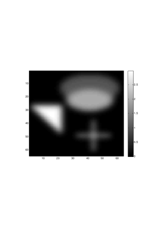
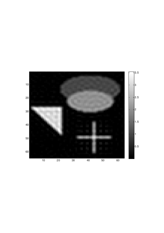
(a)	(b)

Fig. 2: Example 1. Noise level $0.01\%$. Blurred and noisy image (a) and image restored with the proposed preconditioner (b).

We add to the blurred image determined by blur.m a noise vector $e$ with normally distributed random entries with mean zero. The vector is normalized to correspond to a specified noise level. The pixels of the noise- and blur-contaminated image are ordered column-wise and stored in the right-hand side vector $\mbox{\boldmath{$b$}}\in{\mathbb{R}}^{64^{2}}$. First consider $0.1\%$ noise. Then the parameter $p$ for the proposed BCCB preconditioner has the value $14$; it is defined using (12). The discrepancy principle prescribes $k=18$ iterations. This yields a restored image with relative error $0.3404$. Figure 1 displays both the available blur- and noise-contaminated image and the computed restoration. When no preconditioner is used, the discrepancy principle terminates the iterations after $k=33$ steps. The restoration so obtained has relative error $0.3361$. It cannot be distinguished visually from the restoration determined by preconditioned iterations. We therefore do not display the former. We conclude that preconditioning reduces the number of iterations and therefore the computational effort by more than a half and gives a restoration of about the same quality as unpreconditioned iterations. Table 1 displays the $p$-values used and the number of iterations required for $0.1\%$, $0.05\%$, and $0.01\%$ noise in $b$. The noise- and blur-contaminated image together with the restoration determined by preconditioned iterations for the smallest noise level are displayed in Figure 2.

Example 2. We use the same blur and relative noise as in the previous example, but now use the test image “Ken”. For this image, $n_{1}=n_{2}=136$. The BTTB matrix $T$ was generated by the MATLAB function blur.m from [11] with the same parameter values as in the previous example. We add $0.1\%$, $0.05\%$, and $0.01\%$ white Gaussian noise to the blurred image to obtain a blur- and noise-contaminated image, which is stored in the right-hand side vector $\mbox{\boldmath{$b$}}\in{\mathbb{R}}^{136^{2}}$. Table 2 displays the number of iterations required with and without preconditioner to satisfy the discrepancy principle and the $p$-values that define the preconditioners for different noise levels. Figure 3 displays the contaminated and restored images for the noise level $0.1\%$ and Figure 4 shows the contaminated and restored images for the noise level $0.01\%$. Similarly as for Example 1, preconditioned and unpreconditioned iterations give restorations of essentially the same quality. We therefore only show the restoration determined by preconditioned iterations.

% relative data error	$p$	steps $k$	$\|\mbox{\boldmath{$x$}}_{k}-\widehat{\mbox{\boldmath{$x$}}}\|/\|\widehat{\mbox{\boldmath{$x$}}}\|$
$0.10$	$27$	$16$	$0.0764$
$0.10$	$-$	$21$	$0.0726$
$0.05$	$30$	$16$	$0.0691$
$0.05$	$-$	$28$	$0.0673$
$0.01$	$35$	$24$	$0.0571$
$0.01$	$-$	$54$	$0.0575$

Table 2: Example 2: “Ken”. A hyphen signifies that no preconditioner is used.

(a)	(b)

Fig. 3: Example 2. Noise level $0.1\%$. Blurred and noisy image (a) and image restored with the proposed preconditioner (b).

Finally, consider the situation when the zero vector is chosen as initial approximate solution for the preconditioned iterations instead of the vector (8). The parameter $p$ that defines the preconditioner is given by (12) and the iterations are terminated by the discrepancy principle. Then for noise level $0.1\%$, the discrepancy principle prescribes $k=20$ iterations and gives a restoration with relative error $0.0904$. The noise level $0.05\%$ requires $k=21$ iterations and gives a restoration with relative error $0.0776$, and the noise level $0.01\%$ demands $k=28$ iterations and gives a restoration with relative error $0.0596$. A comparison with Table 2 shows that the initialization (8) requires fewer iterations and gives restorations of higher quality than when using the initial vector ${\mbox{\boldmath{$x$}}}_{0}={\mbox{\boldmath{$0$}}}$.

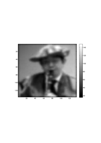
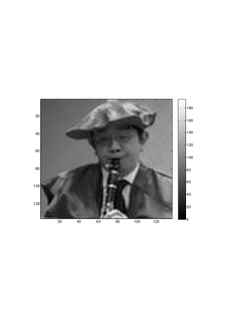
(a)	(b)

Fig. 4: Example 2. Noise level $0.01\%$. Blurred and noisy image (a) and image restored with the proposed preconditioner (b).

Example 3. Our last example is the problem gravity from [11]. The linear system of equations (1) is obtained by discretizing an integral equation of the first kind with a space invariant kernel. This yields a Toeplitz matrix $T\in{\mathbb{R}}^{256\times 256}$ and right-hand side $\widehat{\mbox{\boldmath{$b$}}}\in{\mathbb{R}}^{256}$ to which we add an error vector ${\mbox{\boldmath{$e$}}}\in{\mathbb{R}}^{256}$ to obtain the right-hand side of (1); see (2). The error vector has normally distributed entries with mean zero and is scaled to correspond to the noise levels $0.1\%$, $0.05\%$, or $0.01\%$. The noise level $0.1\%$ gives the parameter $p=3$ for the circulant preconditioner and the discrepancy principle is satisfied after $k=8$ iterations. We obtain the approximation ${\mbox{\boldmath{$x$}}}_{8}$ of the desired solution $\widehat{\mbox{\boldmath{$x$}}}$ with relative error $0.0144$. Without a preconditioner, the same number of iterations are required to satisfy the discrepancy principle and the approximate solution obtained has a larger relative error, namely $0.0160$. Table 3 summarizes the results for all noise levels considered. In this example, the preconditioner does not reduce the number of iterations required to satisfy the discrepancy principle, but improves the quality of the computed solution.

In the computations reported in Table 3, we used the initial iterate (8). If instead the initial iterate $\mbox{\boldmath{$x$}}_{0}={\mbox{\boldmath{$0$}}}$ is used for the preconditioned iterations, then the discrepancy principle is for the noise level $0.1\%$ satisfied after $k=9$ iterations and gives an approximate solution with relative error $0.0316$. When the noise level is reduced to $0.05\%$, the discrepancy principle prescribes that $k=10$ iterations be carried out, resulting in an approximate solution with relative error $0.0222$ and, finally, for noise level $0.01\%$, $k=11$ iterations are needed to satisfy the discrepancy principle and the computed approximate solution has relative error $0.0160$. Thus, for all noise levels the initial iterate $\mbox{\boldmath{$x$}}_{0}={\mbox{\boldmath{$0$}}}$ requires more iterations and gives approximate solutions of inferior quality than the initial iterate (8).

% relative data error	$p$	steps $k$	$\|\mbox{\boldmath{$x$}}_{k}-\widehat{\mbox{\boldmath{$x$}}}\|/\|\widehat{\mbox{\boldmath{$x$}}}\|$
$0.10$	$3$	$8$	$0.0144$
$0.10$	$-$	$8$	$0.0160$
$0.05$	$3$	$9$	$0.0105$
$0.05$	$-$	$9$	$0.0119$
$0.01$	$3$	$10$	$0.0077$
$0.01$	$-$	$10$	$0.0078$

Table 3: Example 3: gravity. A hyphen signifies that no preconditioner is used.

4 Conclusion and extension

This paper presents a novel method to determine BCCB preconditioners to be used for iterative solution of discretized linear ill-posed problem with a BTTB matrix. The computed examples show that the number of iterations is reduced by roughly a half when using the proposed preconditioner, whereas the quality of the computed solution is about the same as without preconditioning.

Also, we would like to mention that instead of using the circulant preconditioners described, one may use the generalized optimal circulant preconditioners described in [15] at the same computational cost. This may be attractive for certain Toeplitz and BTTB matrices.

References

- [1] R. H.-F. Chan and X.-Q. Jin, An Introduction to Iterative Toeplitz Solvers, SIAM, Philadelphia, 2007.
- [2] T. Chan, An optimal circulant preconditioner for Toeplitz systems, SIAM J. Sci. Statist. Comput., 9 (1988), pp. 766–771.
- [3] T. Chan and J. A. Olkin, Circulant preconditioners for Toeplitz-block matrices, Numer. Algorithms, 6 (1994), pp. 89–101.
- [4] F. Di Benedetto, C. Estatico, and S. Serra Capizzano, Superoptimal preconditioned conjugate gradient iteration for image deblurring, SIAM J. Sci. Comput., 26 (2005), pp. 1012–1035.
- [5] L. Dykes, F. Marcellán, and L. Reichel, The structure of iterative methods for symmetric linear discrete ill-posed problems, BIT, 54 (2014), pp. 129–145.
- [6] L. Dykes and L. Reichel, A family of range restricted iterative methods for linear discrete ill-posed problems, Dolomites Research Notes on Approximation, 6 (2013), pp. 27–36.
- [7] H. W. Engl, M. Hanke, and A. Neubauer, Regularization of Inverse Problems, Kluwer, Dordrecht, 1996.
- [8] M. Hanke and J. G. Nagy, Restoration of atmospherically blurred images by symmetric indefinite conjugate gradient techniques, Inverse Problems, 12 (1996), pp. 157–173.
- [9] M. Hanke, J. Nagy, and R. Plemmons, Preconditioned iterative regularization for ill-posed problems, in: L. Reichel, A. Ruttan, and R. S. Varga, eds., Numerical Linear Algebra, de Gruyter, Berlin, 1993, pp. 141–163.
- [10] P. C. Hansen, Rank-Deficient and Discrete Ill-Posed Problems, SIAM, Philadelphia, 1998.
- [11] P. C. Hansen, Regularization tools version 4.0 for Matlab 7.3, Numer. Algorithms, 46 (2007), pp. 189–194.
- [12] M. K. Ng, Iterative Methods for Toeplitz Systems, Oxford University Press, Oxford, 2004.
- [13] S. Kindermann, Convergence analysis of minimization-based noise level-free parameter choice rules for linear ill-posed problems, Electron. Trans. Numer. Anal., 38 (2011), pp. 233–257.
- [14] A. Neuman, L. Reichel, and H. Sadok, Implementations of range restricted iterative methods for linear discrete ill-posed problems, Linear Algebra Appl., 436 (2012), pp. 3974–3990.
- [15] S. Noschese and L. Reichel, The structured distance to normality of Toeplitz matrices with application to preconditioning, Numer. Linear Algebra Appl., 18 (2011), pp. 429–447.
- [16] M. Redivo–Zaglia and G. Rodriguez, smt: a Matlab toolbox for structured matrices, Numer. Algorithms, 59 (2002), pp. 639–659.
- [17] L. Reichel and G. Rodriguez, Old and new parameter choice rules for discrete ill-posed problems, Numer. Algorithms, 63 (2013), pp. 65–87.
- [18] Y. Saad, Iterative Methods for Sparse Linear Systems, 2nd ed., SIAM, Philadelphia, 2003.
- [19] C. van der Mee, G. Rodriguez, and S. Seatzu, Fast computation of two-level circulant preconditioners, Numer. Algorithms, 41 (2006), pp. 275–295.
- [20] C. van der Mee, G. Rodriguez, and S. Seatzu, Fast superoptimal preconditioning of multiindex Toeplitz matrices, Linear Algebra Appl., 418, (2006), pp. 576–590.