Dependence of the Sunspot-group Size on the Level of Solar Activity and its Influence on the Calibration of Solar Observers

1 Introduction

Sec:Intro The sunspot number series was introduced in the 1860s by Rudolf Wolf of Zürich and became the most commonly used index of long-term solar variability ever since. The sunspot number series is longer than 400 years, including the Maunder minimum (Eddy, 1976; Sokoloff, 2004; Usoskin et al., 2015), and is composed of observations from a large number of different observers. Since they used different instruments and different techniques for observing and recording sunspots, it is unavoidable that data from different observers need to be calibrated to each other to produce a homogeneous dataset. The first inter-calibration of data from different observers was performed by Rudolf Wolf in the mid-19th century. He proposed a simple linear scaling between the different observers (the so-called $k-$factors) so that the data (count of groups and sunspots) from one observer should be multiplied by a $k-$factor to rescale it to another reference observer. The value of the correction $k-$factor is assumed to be rigidly fixed, as found by a linear regression, for each observer, and it characterizes the observer’s quality in a relative way with respect to the reference observer. Since then, this method has always been used until very recently (Clette et al., 2014; Svalgaard and Schatten, 2016).

The $k-$factor approach utilizes the method of ordinary linear least square regression forced through the origin. This method is based on several formal assumptions which are usually not discussed, but their violation may lead to incorrect results:

1. Linearity, i.e. the relation between two variables $X$ and $Y$ can be described as linear in the entire range of the $X$-values. This assumption is invalid for the sunspot (group) numbers, as shown by Lockwood et al. (2016a) or Usoskin et al. (2016) and discussed here, because of the essential nonlinearity.

2. Random sample, i.e. the pairs of $X$- and $Y$-values are taken randomly from the same population and have sufficient lengths. This assumption is valid in this case.

3. Zero conditional mean, i.e. normality and independence of errors, implying that all errors are normally distributed around the true values. This assumption is also invalid since the errors are asymmetric and not normal (Usoskin et al., 2016).

4. Constant variance (homoscedasticity). This assumption is violated since the variance of the data is not constant but depends on the level of solar activity so that the variance of the data points is much larger for periods of high activity than around solar minima.

5. X-values are supposed to be known exactly without errors. This assumption is invalid since data from the calibrated observer (X-axis) can be even more uncertain than those by the reference observer (Y-axis).

6. Additionally, forcing through the origin is assumed for the $k-$factors. This assumption is also invalid as shown by Lockwood et al. (2016a), since no spot reported by an observer does not necessarily mean that an observer with a better instrument would not see some small spots.

We do not discuss here the issue of collinearity, since this assumption is not directly applied to the regression problem considered here. Accordingly, five out of six assumptions listed above are invalid in the case of sunspot numbers making the linear scaling calibration by $k-$factor formally invalid. This method was reasonable in the mid-19th century for interpolations to fill short gaps in observations, but now we aim to develop a more appropriate method for a direct calibration of different observers to each other. Several indirect methods of solar-observer calibration have been introduced recently (Friedli, 2016a; Usoskin et al., 2016) but here we focus on a direct inter-calibration based on modern statistical methods.

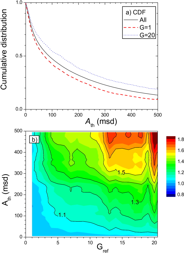
Figure 1.: Size distribution of sunspot groups from the reference database. Panel a: Cumulative distribution function (CDF) of sizes of sunspot groups above the given threshold $A_{\rm th}$. The solid line depicts the entire population of sunspot groups, the red dashed and blue dotted lines show the CDF for low-activity ($G=1$) and high-activity days ($G=20$), respectively. Panel b: The 2D map of the CDF (color code is shown on the right) as a function of the activity level (the daily $G_{\rm ref}$ – X-axis) and the group size (Y-axis), normalized to the CDF at $G=1$ (the red dashed curve in panel a). Fig:map

It was proposed recently (Lockwood et al., 2016a; Usoskin et al., 2016) that the “quality” of a solar observer can be quantified not by a relative $k-$factor but by the observational acuity threshold, i.e. the minimum size of a sunspot group the observer can see considering the used instrumentation, technique and eyesight. This quantity [$A_{\rm th}$] (in millions of the solar disc, msd) has a clear meaning – all sunspot groups bigger than $A_{\rm th}$ are reported while all the groups smaller than $A_{\rm th}$ are missed by the observer. We note that weather conditions and age or experience may lead to variations of the actual threshold for a given observer in time, but here we consider that the threshold is constant in time. This is also assumed in the $k-$factor methodology. The threshold would be consistent with the $k-$factor if the fraction of small ($<A_{\rm th}$) groups on the solar disc was roughly constant and independent on the level of solar activity. However, as many studies imply (Kilcik et al., 2011; Jiang et al., 2011; Nagovitsyn, Pevtsov, and Livingston, 2012; Obridko and Badalyan, 2014), the fraction of small groups varies with solar activity: it is large around solar minima and decreases with the level of solar activity. Accordingly, the use of the linear $k-$factor method may lead to a distortion of the calibrated sunspot numbers (Lockwood et al., 2016b).

In this article we study the relation between sunspot group counts by a “poor” observer and those by the reference “perfect” observer, using the reference dataset described in Section Sec:data. In Section Sec:dist we study the distribution of sunspot group sizes and its dependence on the level of solar activity. Its effect on observations by solar observers of different quality and their inter-calibrations are discussed in Section Sec:obs. We propose the use of a new nonlinear $c-$factor to calibrate data from a “poor” observer to the reference conditions depending on the level of solar activity, in a more realistic manner than that offered by the traditionally used linear $k-$factor.

2 Data

Sec:data

We base our analysis on the Royal Greenwich Observatory (RGO) data series of sunspot groups with their areas. This series is referred to as the reference dataset throughout this article. Although the RGO data series starts in 1874, there are indications that its quality might be variable before 1900 (Clette et al., 2014) or even before 1915 (Cliver and Ling, 2016) due to the “learning” curve, although other studies did not find this effect or attributed it only to the very early part of the RGO record before 1880 (Sarychev and Roshchina, 2009; Carrasco et al., 2013; Aparicio et al., 2014). To stay on the conservative safe-side, we consider here RGO data only for the period 1916–1976 when the data series is homogeneous in quality. We have checked that the result remains qualitatively the same if the period of 1874–1915 is included into the analysis. Since the RGO series was terminated in 1976, we also stop our reference dataset at that time, not extending it with data from the Solar Observing Optical Network (SOON) because of a possible transition inhomogeneity (Lockwood, Owens, and Barnard, 2014; Hathaway, 2015).

To make the results compatible with the direct observations, we used in our analysis the uncorrected (for foreshortening) whole area of sunspot groups, i.e. as it is seen from Earth. We consider sunspot groups, not individual spots, since several closely located spots indistinguishable by the observer can be seen as one blurred spot even with a poor telescope and thus are more representative for the actual data.

From the reference RGO data series we compiled files of daily numbers of sunspot groups with different observational acuity thresholds [$A_{\rm th}$] quantified as the group areas in msd, so that a group is counted (observed) if its uncorrected total area is not smaller that the threshold value in msd. The corresponding daily number of groups is denoted as $G_{\rm A}(t)$ where the subscript $A$ denotes the value of the threshold in msd. For example $G_{100}$ denotes the number of groups with area $\geq 100$ msd for each day. The number of groups without applying any threshold ($A_{\rm th}=0$, i.e. the total number of groups in the reference dataset irrespectively of their size) is called the reference series $G_{\rm ref}$.

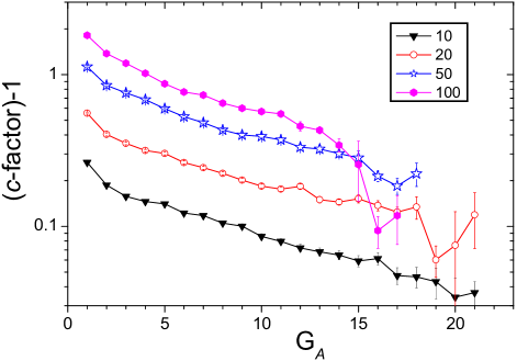
Figure 2.: Ratio of the “small” (viz. smaller than the given value of the threshold [$A_{\rm th}$] in units of msd as denoted in the legend) to “large” sunspot groups as a function of the number of ‘large’ groups, in the total daily number of sunspot groups for the RGO dataset for the period 1916–1976. This corresponds to the correction $c-$factor (see text) minus 1. The error bars represent the standard statistical errors of the ratio. Fig:CF

For the analysis of data by Rudolf Wolf and Alfred Wolfer (Section Sec:WW) we used the daily number of sunspot groups as presented in the database of Hoyt and Schatten (1998) and the new revised collection of sunspot group numbers by Vaquero et al. (2016), for the period of their overlap 1876-1893. However, the latest (not available for the time of making the present analysis) revision of the Wolf’s records (Friedli, 2016b) is not included in these two databases. On the other hand, the analysis of Wolf and Wolfer data is shown for illustration and would not be altered with the slightly revised dataset.

3 Distribution of Sunspot-group Sizes

Sec:dist

Here we investigated how size of sunspot groups changes with solar activity. This is usually studied using the mean size of sunspot groups (Jiang et al., 2011) but this may be confusing because the size distribution of spots is highly asymmetric and the mean value is not a robust feature.

Figure Fig:mapa depicts the cumulative distribution function (CDF) of sunspot-group sizes (uncorrected total area in msd) for the reference dataset (Section Sec:data). CDF($A_{\rm th}$) is defined as the fraction of the sunspot groups with area not smaller than the given value of the area threshold [$A_{\rm th}$]. By definition CDF(0) is equal to unity (each group has a non-zero size). The black curve shows the global CDF for all the sunspot groups (about 119300 groups) in the reference dataset. The blue dotted line represents the CDF for 920 groups (46 days) for high activity days with 20 groups ($G=20$) reported. The red dashed curve depicts the CDF for 2781 days with low activity (only one group reported, $G=1$). One can see that there is a significant fraction of large groups even for low-activity days: $\approx$10% of groups have area greater than 500 msd. The group-size distribution changes with the level of solar activity: while the CDF for low-activity days is lower than the global CDF, the distribution for high-activity days is significantly higher. For example, as one can see from Figure Fig:mapa, the relative contribution of large sunspot groups ($A\geq 500$ msd) doubles for high-activity days ($G=20$) with respect to low-activity days ($G=1$). This implies that the rise of activity is mostly due to the emergence of large sunspot groups, indicating that the sunspot-group size distribution changes with the level of solar activity.

To generalize the study of the CDF dependence on the level of solar activity, we plotted in Figure Fig:mapb a contour plot of the CDF as a function of the activity level (quantified in $G$) and the group size (quantified in msd). All the CDF were normalized to that at the low-activity level ($G=1$, see red dashed line in Figure Fig:mapa) so that CDF($G=1$) is unity for all $A_{\rm th}$. One can see that the shape of CDF changes with the level of solar activity so that the fraction of large spots is growing, while the fraction of small spot decreases with activity. For example, the brown spot in the top-right corner implies that the relative fraction of groups with area $>500$ msd is nearly doubled for high-activity days ($G=20$) compared to low-activity days ($G=1$), as discussed above for Figure Fig:mapa.

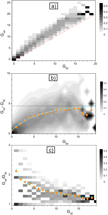
Figure 3.: Relation between daily sunspot-group numbers as counted by a ‘perfect’ observer $G_{\rm ref}$ and by an observer with the acuity threshold $A_{\rm th}=50$ msd, $G_{50}$, using data from the reference data set. Panel a: The PDF of the scatter plot of $G_{\rm ref}$ vs. $G_{50}$. The red dashed line marks the diagonal. Panel b: The difference ($G_{\rm ref}-G_{50}$) vs. $G_{50}$. The orange dots with error bars depict the mean values (with the asymmetric errors of the mean) of the difference in each PDF strip for fixed $G_{50}$. The cyan line is the best fit Equation (Eq:exp), while the horizontal dashed line is the value of $R_{\infty}$. Panel c: The correction factor, $c_{50}\equiv G_{\rm ref}/G_{50}$ vs. $G_{50}$. The orange dots with error bars depict the mean values (with the errors of the mean) of the difference in each PDF strip for fixed $G_{50}$. The cyan line corresponds to that in panel b. The color code for all PDFs is shown on the right. Fig:rgo50

In the subsequent section we study how the fact that the size distribution of sunspot groups changes with the level of solar activity affects solar observers of different quality and their mutual inter-calibration.

4 Observer’s View

Sec:obs

4.1 “Imperfect” vs. “perfect” observers

Sec:imp We assume (similar to Lockwood et al., 2016a and Usoskin et al., 2016) that a solar observer is imperfect and has an observational acuity threshold [$A_{\rm th}$] for the (uncorrected for foreshortening) sunspot-group area so that he/she reports all the groups bigger than $A_{\rm th}$ and miss all the groups smaller than $A_{\rm th}$. Accordingly, we simulated a set of sunspot-group records produced by pseudo-observers synthesized from the reference dataset and characterized only by the acuity threshold [$A_{\rm th}$].

We define the “correction factor” $c_{A}$ as the ratio of the number of sunspot groups $G_{\rm ref}$ reported by the perfect observer ($A_{\rm th}=0$) to that $G_{A}$ by an imperfect observer with the finite acuity threshold [$A$] ($A_{\rm th}=a$), as a function of $G$:

$$c_{A}(G_{A})\equiv{G_{\rm ref}\over G_{A}}.\ilabel{Eq:ca}$$ (1)

Figure Fig:CF depicts ($c_{A}$-1) as function of $G_{A}$ for several values of the threshold $A_{\rm th}$. One can see that the relative observational errors (the fraction of missed sunspot groups to the “true” number of groups) of a “poor” observer rapidly decrease with the level of solar activity. For example, while the observer with $A_{\rm th}=100$ msd would count roughly ²/₃ less groups at very low activity $G_{100}=1$, the fraction of missed small groups is only 20-25% for the high activity days $G_{100}=15$. It is obvious that applying a constant correction factor (as used in the $k-$factor method) is inappropriate, since this would distort the entire series and overcorrect the periods of high solar activity. Here we introduce the $c-$factor to correct sunspot-group counts by an “imperfect” observer to the reference observer. The concept of the $c-$factor is similar to that of the $k-$factor but depends on the level of solar activity quantified as $G_{A}$.

In Figure Fig:rgo50 we depict the relation between the reference and “poor” observers for the acuity threshold of $A_{\rm th}=50$ msd. Panel a shows the conversion matrix for the reference observer and the one with $A_{\rm th}$, constructed in the same way as by Usoskin et al. (2016), for all days during the period 1916–1976. The matrix represents the statistics of the reported $G-$values for the two observers, normalized to unity in each column so that it represents the probability density function (PDF) of the number of groups reported by the reference observer $G_{\rm ref}$ for the days when the poor observer reported $G_{50}$ groups. One can see that the poor observer always counts less groups than the reference one (all shaded areas lie above the diagonal), but the shape of the relation is not clear and could seemingly be approximated by a straight line.

To verify our previous assertion, we show in Figure Fig:rgo50b the PDF for the difference between the observers, i.e. $D_{50}=(G_{\rm ref}-G_{50})$ as a function of $G_{50}$. One can see that the relation is essentially nonlinear but bends to become flat at high activity. While the actual spread of the distribution (grey shading) is wide, this feature is clearly visible from the mean values (orange dots on the plot) of $D_{50}$ that form a smooth curve which tends to reach a saturation at high values of $G_{50}$. This relation is very smooth and we approximate it with a simple euqation

$$D_{A}(G_{A})=R_{\infty}-(R_{\infty}-R_{0})\,\exp(-\alpha\,G_{A}),\ilabel{Eq:exp}$$ (2)

where $R_{0}=D_{A}(0)$ is the mean value of $G_{\rm ref}$ at $G_{A}=0$, $R_{\infty}$ is the asymptotic value (shown as the horizontal dotted line in Fig. Fig:rgo50b), and $\alpha$ defines the exponential rate. We note that $R_{0}$ represents the mean number of sunspot groups reported by the reference observer for days when the “poor” observer reports no sunspot group. For this particular case, $R_{0}=0.64_{-0.01}^{+0.03}$ implying that on average the reference observer sees 0.64 sunspot groups on days when the “poor” observer with $A_{\rm th}=50$ msd reports no groups because of their small size.

Since the value of $R_{0}$ is fixed for a given observer, Equation (Eq:exp) includes two free parameters $\alpha$ and $R_{\infty}$. We fitted this relation to the mean values of $D_{A}$ (orange dots in Fig. Fig:rgo50b) using the $\chi^{2}$ method. The best-fit parameters for the dependence shown in Fig. Fig:rgo50b are: $\alpha=0.15\pm 0.01$, $R_{\infty}=4.89\pm 0.22$. The value of $\chi^{2}$ for 14 degrees of freedom (DoF) is 15, implying a good fit.

The correction factor $c_{A}(G_{A})$ (see Equation Eq:ca) can be computed from the difference $D_{A}$ as

$$\ilabel{Eq:cf}c_{A}(G_{A})\equiv{G_{\rm ref}\over G_{A}}={D_{A}\over G_{A}}+1,\ilabel{Eq:CC}$$ (3)

as shown in Fig. Fig:rgo50C. The proposed empirical relation (blue curve) describes the dependence of $c_{A}$ on $G_{A}$ quite well. We note that this curve was not fitted again to the data points but simply recalculated from that shown in panel b. The value of $c_{A}$ is not defined for $G_{A}=0$.

4.2 Empirical Dependence

Sec:emp We have repeated the exercise described in Section Sec:imp, i.e. fitting Equation Eq:exp to the difference $D_{A}$, for different values of the observational acuity threshold [$A_{\rm th}$] from 10 to 200 msd. This range corresponds to actual observers with proper telescopes (Vaquero and Vázquez, 2009; Arlt et al., 2013; Neuhäuser et al., 2015; Usoskin et al., 2016). Generally, an observer with the visual acuity threshold exceeding 100 msd would be considered as one with very poor quality.

Some examples of the fits are shown in Figure Fig:fits for several values of $A_{\rm th}$. Although the fits were actually done for the $D_{A}(G_{A})$ distributions (similar to that shown in Fig. Fig:rgo50b), we show here the $c-$factors. We see that the equation fits the data almost perfectly when the statistic is good but the errors bars of the data points increase for higher values of $G_{A}$ because of a poorer statistic. . The fit is always good in the entire range of the $A_{\rm th}$ values analyzed here, and the values of $\chi^{2}$ are typically around 1 per DoF with a variability between 0.5 and 1.5 per DoF, indicating a good agreement.

It is interesting to note that the best-fit curves tend to slightly overestimate the $c-$factor for the highest activity periods (see Figure Fig:fits). This implies that an “imperfect” observer appears not as bad as it should be according to its acuity limitation. However, this tendency is not statistically significant, and we do not consider it in this study. Since we use the method of minimizing $\chi^{2}$ to fit the curve, the contribution of these points is small.

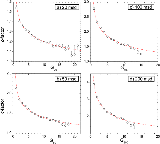
Figure 4.: The correction $c-$factors for different values of the acuity threshold [$A_{\rm th}$] as indicated in the insets. Only the means with their standard errors are shown (see Fig. Fig:rgo50c) as open circles. The red dashed curves are the best-fit relations given by Equation Eq:cf. Fig:fits

The dependence of the parameters of the empirical relation on the value of $A_{\rm th}$ is shown in Figure Fig:par. One can see a smooth growth of the parameters with increasing acuity threshold. The parameter $R_{0}$ raises from its obvious zero value to nearly 1.5. The parameter $R_{\infty}$ grows from its obvious zero value to about eight and tends to saturate there. The parameter $\alpha$ varies between 0.15 and 0.27.

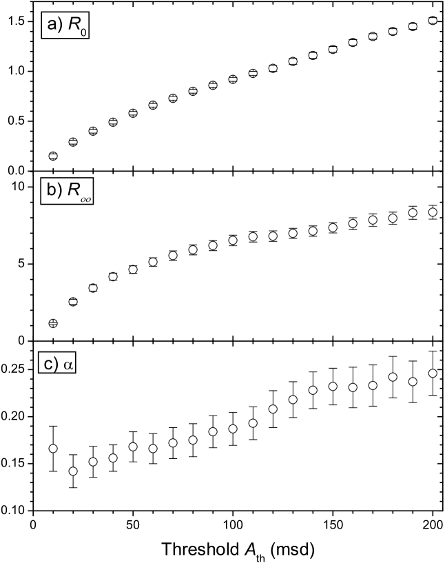
Figure 5.: Dependence of the best-fit parameters of Equation (Eq:exp) on the acuity threshold [$A_{\rm th}$], using the reference dataset. The parameters are shown with the 68% confidence interval ($1\sigma$) uncertainties. Fig:par

The empirical relation studied here (Equations Eq:exp–Eq:CC) implies that the fraction of small sunspot groups is not constant as a function of solar activity level, but declines exponentially with the activity as is apparent from Figure Fig:fits. Over the solar cycle, the number of sunspot groups increases mostly because of large groups, while the amount of small groups remains nearly constant in accordance with the analysis presented in Section Sec:dist.

4.3 A Test: Wolf vs. Wolfer

Sec:WW

Here we study the relation between the sunspot-group numbers reported by two classical sunspot observers of the second half of the 19th century: Rudolf Wolf and Alfred Wolfer, both from Zürich Observatory. They were primary observers for the Wolf (and its successor the International) sunspot number series and thus defined the values of the sunspot numbers the late 19th and earlier 20th centuries. A scaling $k-$ factor of 1.66 is traditionally applied to the sunspot (group) number by Wolf to match it with Wolfer in quality, as initially proposed by Wolfer himself. This factor was used continuously (Clette et al., 2014; Svalgaard and Schatten, 2016) in the daisy-chain procedure to calibrate the sunspot number series ever since. Thus, it is important to verify the inter-calibration of the two observers. We use all the days (4385 in total) when we have observations from both observers for the period 1876–1893. This analysis is close to that of Usoskin et al. (2016) but is focused on the use of the proposed parameterization (Equation (Eq:exp)).

Figure Fig:WWa shows a conversion matrix, constructed in the same way as that in Figure Fig:rgo50 but for the Wolfer vs. Wolf data, so that Wolfer is now the reference observer and Wolf is a “poor” one. One can see that Wolfer was indeed a better observer than Wolf since he reported more groups than Wolf did, for the same days. This is shown by as the grey area in Figure Fig:WWa that lies systematically above the diagonal (red dotted line). On the other hand, the blue dashed line (the $k-$factor of 1.66) lies systematically above the grey area for $G_{\rm Wolf}>4$.

Figure Fig:WWb depicts the difference $G_{\rm Wolfer}-G_{\rm Wolf}$ as function of $G_{\rm Wolf}$, similar to Figure Fig:rgo503. One can see that the relation between the number of groups reported by the two observers is not linear, but again has the same shape of an asymptotic approach to the constant difference. The value of $R_{0}$ was found to be $0.401_{-0.13}^{+0.06}$, implying that Wolfer on average reported 0.4 sunspot groups for days when Wolf reported none, due to the difference in the instrumentation and eyesight. Mean values of the distribution (orange balls in the figure) can be fitted well by Equation (Eq:exp) with $R_{\infty}=2.43$. The linear relation ($k-$factor of 1.66, the blue dashed line) does not describe the relation in a reasonable way as it systematically overestimates the corrected Wolf’s records for days with mid- and high-activity ($G_{\rm Wolf}>4$).

Figure Fig:WWc shows the correction factor ($G_{\rm Wolfer}/G_{\rm Wolf}$) as a function of $G_{\rm Wolf}$. It is obviously nonlinear: while Wolf underestimated (comparing to Wolfer) the number of groups by a factor of two during the low activity periods (one sunspot group per day), his under-count of groups was only 20% for the days with a number of groups exceeding eight. Accordingly, the assumption of the constancy of the correction $k-$factor at the level of 1.66 (the blue dashed line) is invalid in this case.

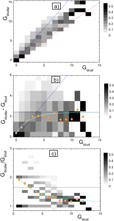
Figure 6.: Similar to Figure Fig:rgo50 but for the relation between group numbers as reported by Wolfer, $G_{\rm Wolfer}$, and Wolf, $G_{\rm Wolf}$. The blue dashed lines in all panels denote the constant scaling $k-$fator of 1.66 often used to scale Wolf to Wolfer. Fig:WW

A principle assumption behind the $k-$factor methodology (see Section Sec:Intro) is that the relation between the number of sunspots (groups) reported by different observers is linear. However, as shown here for the example of two famous observers, the relation between the number of sunspot groups reported by them is essentially nonlinear and, when applying the constant $k-$factor, leads to underestimate of the number of groups during low activity but overestimate is during high activity periods. This is illustrated in Figure Fig:Aug93, where daily group numbers are shown for August 1893 (a month with high activity) by both observers: the original group counts by Wolfer, the counts by Wolf corrected using the constant $k-$factor of 1.66, and the counts by Wolf corrected using Equation (Eq:exp). We see that for the period from 6th to 26th of August, when the temporal profiles of the number of groups by Wolf and Wolfer were close to each other, indicating that they reported the same sunspot activity evolution, the correction based on the $k-$factor yields a good agreement for the days with moderate activity ($G_{\rm Wolfer}<8$) but systematically overestimates counts by 3–4 groups (40–60%) for the days with high activity ($G_{\rm Wolfer}>10$). On the other hand, the nonlinear method proposed here reproduces the level for the entire period correctly.

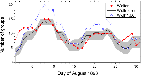
Figure 7.: Daily number of sunspot groups for August 1893. The red curve depicts the number of groups reported by Wolfer, the black curve with its 68% confidence interval denotes the data by Wolf normalized to Wolfer by the method described here, and the blue dotted curve is the data by Wolf scaled by the $k-$factor 1.66. Fig:Aug93

5 Conclusions

We have studied the distribution of sunspot group size or area and its dependence on the level of solar activity. We show that the size distribution of sunspot groups cannot be assumed constant but varies significantly with solar activity. The fraction of small groups, which can be potentially missed by an “imperfect” solar observer, is found to be not constant but decreasing with the level of solar activity. An empirical relation (Equation (Eq:exp)) is proposed which describes the amount of small groups as a function of the solar activity level. It is shown that the number of small groups asymptotically approaches a saturation level so that high solar activity is largely defined by big groups.

We have studied the effect of the changing sunspot group area on the ability of realistic observers to see and report the daily number of sunspot groups. It is shown that the relation between the numbers of sunspot groups as seen by different observers with different observational acuity thresholds (defined by the quality of their instrumentation and eye sights) is strongly non-linear and cannot be approximated by a linear scaling, in contrast to how it was traditionally done earlier. We propose to use the observational acuity threshold $A_{\rm th}$ to quantify the quality of each observer, instead of the relative $k-$factor used earlier. The value of $A_{\rm th}$ means that all sunspot groups bigger than $A_{\rm th}$ would be reported while all the groups smaller than $A_{\rm th}$ missed by the observer. We have introduced the non-linear $c-$factor, based on the observer’s acuity threshold $A_{\rm th}$, which can be used to correct each observer to the reference conditions.

The method has been applied to a pair of principal solar observers of the 19th century, Rudolf Wolf and Alfred Wolfer of Zürich. We have shown that the earlier used linear method to correct Wolf data to the conditions of Wolfer, using the constant $k-$factor of 1.66, tends to overestimate of solar activity around solar maxima.

This result presents a new tool to recalibrate different solar observers to the reference conditions. A full recalibration based on the new method will be a subject of a forthcoming work.

Disclosure of Potential Conflicts of Interest

The authors declare that they have no conflicts of interest.

References

- Aparicio et al. (2014) Aparicio, A.J.P., Vaquero, J.M., Carrasco, V.M.S., Gallego, M.C.: 2014, Sunspot Numbers and Areas from the Madrid Astronomical Observatory (1876 - 1986). Solar Phys. 289, 4335. DOI. ADS.
- Arlt et al. (2013) Arlt, R., Leussu, R., Giese, N., Mursula, K., Usoskin, I.G.: 2013, Sunspot positions and sizes for 1825-1867 from the observations by Samuel Heinrich Schwabe. Mon. Not. Royal Astron. Soc. 433, 3165. DOI.
- Carrasco et al. (2013) Carrasco, V.M.S., Vaquero, J.M., Gallego, M.C., Trigo, R.M.: 2013, Forty two years counting spots: Solar observations by d.e. hadden during 1890–1931 revisited. New Astron. 25, 95. DOI. ADS.
- Clette et al. (2014) Clette, F., Svalgaard, L., Vaquero, J.M., Cliver, E.W.: 2014, Revisiting the sunspot number: A 400-year perspective on the solar cycle. Space Sci. Rev. 186, 35. DOI.
- Cliver and Ling (2016) Cliver, E.W., Ling, A.G.: 2016, The Discontinuity Circa 1885 in the Group Sunspot Number. Solar Phys.,. DOI. ADS.
- Eddy (1976) Eddy, J.A.: 1976, The Maunder minimum. Science 192, 1189. DOI. ADS.
- Friedli (2016a) Friedli, T.: 2016a, The construction of the Wolf series from 1749 to 1980. Solar. Phys, in press.
- Friedli (2016b) Friedli, T.K.: 2016b, Sunspot Observations of Rudolf Wolf from 1849 - 1893. Solar Phys. in press. DOI. ADS.
- Hathaway (2015) Hathaway, D.H.: 2015, The solar cycle. Living Rev. Solar Phys. 12, 4. DOI. http://www.livingreviews.org/lrsp-2015-4.
- Hoyt and Schatten (1998) Hoyt, D.V., Schatten, K.H.: 1998, Group sunspot numbers: A new solar activity reconstruction. Solar Phys. 179, 189. DOI. ADS.
- Jiang et al. (2011) Jiang, J., Cameron, R.H., Schmitt, D., Schüssler, M.: 2011, The solar magnetic field since 1700. I. Characteristics of sunspot group emergence and reconstruction of the butterfly diagram. Astron. Astrophys. 528, A82. DOI.
- Kilcik et al. (2011) Kilcik, A., Yurchyshyn, V.B., Abramenko, V., Goode, P.R., Ozguc, A., Rozelot, J.P., Cao, W.: 2011, Time Distributions of Large and Small Sunspot Groups Over Four Solar Cycles. Astrophys. J. 731, 30. DOI. ADS.
- Lockwood, Owens, and Barnard (2014) Lockwood, M., Owens, M.J., Barnard, L.: 2014, Centennial variations in sunspot number, open solar flux, and streamer belt width: 1. Correction of the sunspot number record since 1874. J. Geophys. Res., Space Phys. 119, 5172. DOI. ADS.
- Lockwood et al. (2016a) Lockwood, M., Owens, M.J., Barnard, L., Usoskin, I.G.: 2016a, Tests of Sunspot Number Sequences: 3. Effects of Regression Procedures on the Calibration of Historic Sunspot Data. Solar Phys., (in press. DOI. ADS.
- Lockwood et al. (2016b) Lockwood, M., Owens, M.J., Barnard, L., Usoskin, I.G.: 2016b, An assessment of sunspot number data composites over 1845–2014. Astrophys. J. 824(1), 54. DOI.
- Nagovitsyn, Pevtsov, and Livingston (2012) Nagovitsyn, Y.A., Pevtsov, A.A., Livingston, W.C.: 2012, On a Possible Explanation of the Long-term Decrease in Sunspot Field Strength. Astrophys. J. 758, L20. DOI. ADS.
- Neuhäuser et al. (2015) Neuhäuser, R., Arlt, R., Pfitzner, E., Richter, S.: 2015, Newly found sunspot observations by Peter Becker from Rostock for 1708, 1709, and 1710. Astron. Nachr. 336, 623. DOI. ADS.
- Obridko and Badalyan (2014) Obridko, V.N., Badalyan, O.G.: 2014, Cyclic and secular variations sunspot groups with various scales. Astron. Rep. 58, 936. DOI. ADS.
- Sarychev and Roshchina (2009) Sarychev, A.P., Roshchina, E.M.: 2009, Comparison of three solar activity indices based on sunspot observations. Solar Syst. Res. 43, 151. DOI. ADS.
- Sokoloff (2004) Sokoloff, D.: 2004, The maunder minimum and the solar dynamo. Solar Phys. 224, 145. DOI. ADS.
- Svalgaard and Schatten (2016) Svalgaard, L., Schatten, K.H.: 2016, Reconstruction of the Sunspot Group Number: The Backbone Method. Solar Phys., in press. DOI. ADS.
- Usoskin et al. (2015) Usoskin, I.G., Arlt, R., Asvestari, E., Hawkins, E., Käpylä, M., Kovaltsov, G.A., Krivova, N., Lockwood, M., Mursula, K., O’Reilly, J., Owens, M., Scott, C.J., Sokoloff, D.D., Solanki, S.K., Soon, W., Vaquero, J.M.: 2015, The Maunder minimum (1645-1715) was indeed a grand minimum: A reassessment of multiple datasets. Astron. Astrophys. 581, A95. DOI. ADS.
- Usoskin et al. (2016) Usoskin, I.G., Kovaltsov, G.A., Lockwood, M., Mursula, K., Owens, M., Solanki, S.K.: 2016, A New Calibrated Sunspot Group Series Since 1749: Statistics of Active Day Fractions. Solar Phys., in press DOI. ADS.
- Vaquero and Vázquez (2009) Vaquero, J.M., Vázquez, M.: 2009, The Sun Recorded Through History: Scientific Data Extracted from Historical Documents, Astrophys. Space Sci. Lib. 361, Springer, Berlin. ADS.
- Vaquero et al. (2016) Vaquero, J.M., Svalgaard, L., Carrasco, V.M.S., Clette, F., Lefèvre, L., Gallego, M.C., Arlt, R., Aparicio, A.J.P., Richard, J., Howe, R.: 2016, A Revised Collection of Sunspot Group Numbers. Solar Phys., submitted.