Non-equilibrium fluctuations of a semi-flexible filament driven by active cross-linkers

Abstract

The cytoskeleton is an inhomogeneous network of semi-flexible filaments, which are involved in a wide variety of active biological processes. Although the cytoskeletal filaments can be very stiff and embedded in a dense and cross–linked  network, it has been shown that, in cells, they typically exhibit significant bending on all length scales. In this work we propose a model of a semi-flexible filament deformed by different types of cross-linkers for which one can compute and investigate the bending spectrum. Our model allows to couple the evolution of the deformation of the semi-flexible polymer with the stochastic dynamics of linkers which exert transversal forces onto the filament. We observe a $q^{-2}$ dependence of the bending spectrum for some biologically relevant parameters and in a certain range of wavenumbers $q$. However, generically, the spatially localized forcing and the non-thermal dynamics both introduce deviations from the thermal-like $q^{-2}$ spectrum.

In recent years many studies were performed on active gels to investigate their complex and dynamic structure, which shows generic non-equilibrium behavior. The cytoskeleton, an important example of an active gel, is able to form self-organized structures that are the basis of many fundamental processes within cells Alberts et al. (2014); Bray (2000); Howard (2001). The cytoskeleton is composed of actin and intermediate filaments, as well as microtubules, that take important roles for example in cell motility, cell division and intracellular transport Alberts et al. (2014); Stricker et al. (2010). It has been shown that these cytoskeletal filaments can cross-link via static Selden and Pollard (1986) and dynamic interactions Rodriguez et al. (2003); Straube et al. (2006).

Mechanically the cytoskeletal filaments are semi-flexible filaments with very different persistence lengths. In vitro measurements estimated a thermal persistence lengths of the order of $17\mu$m for actin and a few millimeters for microtubules Gittes et al. (1993); van Mameren et al. (2009); Brangwynne et al. (2007a). By contrast, much smaller persistence lengths are observed for microtubules in vivo ($\approx 30\mu m$ in Brangwynne et al. (2007b)). These strong deformations are interpreted to be the result of large non-thermal forces of the order of $1$-$10$pN, which is in the range of individual motors’ strength. While in some experiments it was surprisingly observed that the bending spectrum exhibits the same shape as thermal ones Brangwynne et al. (2007b), other observations reported strong deviations Brangwynne et al. (2008).

Some continuous theoretical descriptions of active networks exist Jülicher et al. (2007); Marchetti et al. (2013); Broedersz and MacKintosh (2014), which allow to study the deformation of an embedded filament Kikuchi et al. (2009), However, it is of great interest to understand how deformations originate from microscopic discrete forcing MacKintosh and Levine (2008); Ronceray and Lenz (2015); Ronceray et al. (2016); Broedersz et al. (2010); Shekhar et al. (2013); Gladrow et al. (2016).

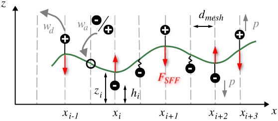
Figure 1: Sketch of the model in the case of active cross-linkers. Cross-linkers (black dots) are connected to the SFF (green) through rope-like chains, which can be fully extended (straight segment) or not (wavy line). With rate $\omega_{\rm a}$, cross-linkers can attach at empty intersections ($\circ$) between the SFF and the background filaments. The SFF exerts some forces $F_{\rm{SFF}}$ (red arrows) on fully extended cross-linkers, which are located at positions $(x_{i},h_{i})$ and impose the vertical positions $z_{i}(x_{i})$ of the SFF. Cross-linkers step upwards or downwards ($(+)$ or $(-)$ labels) along the polarized vertical background filaments, with stepping rate $p\equiv p(F_{\rm{SFF}})$. Cross-linkers detach with rate $\omega_{\rm d}\equiv\omega_{\rm d}(F_{\rm{SFF}})$.

In this paper we consider an idealized system (Fig. 1) in which a set of cross-linkers impose transverse deformations to a semi-flexible filament (SFF). To couple the dynamics of SFF and linkers, we determine at each instant the equilibrium shape of the SFF under the constraints imposed by the cross-linkers. The method also provides the forces exerted by the deformed filament on each cross-linker, allowing to implement some feedback of the SFF onto the stochastic linkers dynamics.

We shall consider two types of linkers, having thermal or non-thermal dynamics. This will allow us to disentangle the geometrical effects from those due to the non-thermal dynamics of active linkers. We apply our algorithm to explore the dependence of the persistence length $L_{\text{p}}$ and of the bending spectrum upon various parameters, including the properties of linkers and of the surrounding network.

We now introduce our model in more details.

Semi-flexible filament – The bending energy $E$ of a SFF of length $L$ with bending rigidity $k$ is given by Landau and Lifshitz (1981)

$$E=k\int_{0}^{L}\left(\frac{\partial\theta}{\partial s}\right)^{2}ds$$ (1)

and depends on the local curvature ${\partial\theta}/{\partial s}$, where $\theta(s)$ is the tangent angle and $s$ the contour length. We shall express the value of $k$ in units of $k_{MT}$, the experimentally measured bending rigidity of microtubules (see Table 1 in Supplementary Material (SM) sm ). In the following, we assume periodic boundary conditions and connect the SFF’s ends to form a ring. Therewith we avoid filament rotation like in vortices Sumino et al. (2012) which are not relevant within the cell context.

Cross-linkers – We consider two types of cross-linkers which are connected to some static background filaments and induce SFF shape fluctuations. The background filaments are all perpendicular to the SFF, with a lattice spacing $d_{\rm{mesh}}$ (see Fig. 1).

Thermal cross-linkers (see Fig. S1 in SM sm ) are permanently bound to the SFF. They step in both directions along the background network and thereby alter the SFF’s shape. A step of a cross-linker, and hence the new SFF shape, is accepted according to the detailed balance condition, i.e., with probability $\min(1,\exp(-\Delta E/k_{B}T))$, where $\Delta E$ is the associated energy change and $k_{B}$ the Boltzmann constant.

Active cross-linkers may bind to or unbind from the SFF. Their binding is not direct but via a small infinitely flexible chain with maximum length $l_{\rm{max}}$. The linker can exert a force only when its chain is extended. An unbound active linker attaches to an available binding site (i.e., an intersection point between the SFF and one background filament) with constant rate $\omega_{\rm a}$. For each attachment event, the stepping direction $(+)$ or $(-)$ of the cross-linker is randomly chosen and kept fixed until it detaches again.

Once attached, the active cross-linker stochastically takes discrete steps along the background filament in the direction determined above. The stepping rate $p(F_{\rm{SFF}})$ depends strongly on the load force $F_{\rm{SFF}}$ exerted by the SFF on the linker (see formulas (S1-S2) in SM sm ). If the load force pulls in opposite direction to the stepping direction of the active linker, the linker velocity is reduced. It stops when the load force exceeds the linker’s stall force $F_{\rm{s}}$. The active linkers stochastically detach with rate $\omega_{\rm d}(F_{\rm{SFF}})=\omega_{{\rm d}_{0}}\exp\left(\frac{|F_{\rm{SFF}}|}{F_{\rm{d}}}\right)$ where $F_{\rm{d}}$ gives the detachment force scale.

Bound cross-linkers with an extended chain can exert a force and possibly deform the SFF, which in turn will apply a restoring force on the linkers. For some deformations of the SFF the restoring force may induce sudden detachments of cross-linkers or even initiate detachment cascades.

The time scale separation of the linker dynamics and SFF relaxation allows the simulation of single linker activity and consecutive instantaneous SFF relaxation. The coupling between the dynamics of SFF and cross-linkers is implemented as follows for both types of linkers (see SM, Section IV sm for more details).

Equilibrium shape of a constrained SFF – The semi-flexible filament’s shape is chosen to minimize the bending energy under the constraints imposed by the pulling cross-linkers. Between two consecutive pulling cross-linkers located in $x_{i}$ and $x_{i+1}$ the SFF shape is given by a profile $u_{i}(x)$, that minimizes the energy (1) of this portion of the SFF

$$E_{i}=k\int_{x_{i}}^{x_{i+1}}\left[\partial_{x}^{2}u_{i}(x)\right]^{2}dx$$ (2)

assuming no overhang and $\left|\partial_{x}u_{i}(x)\right|\ll 1$.

The force per unit length is $F\sim\partial^{4}_{x}u_{i}(x)$, which vanishes at equilibrium between two attachment points. Thus the equilibrium is given by (see for instance Ref. Schwarz and Maimon (2001))

$$u_{i}(x)=a_{i}(x-x_{i})^{3}+b_{i}(x-x_{i})^{2}+c_{i}(x-x_{i})+d_{i}$$ (3)

for $x_{i}\leq x\leq x_{i+1}$. Let $z_{i}$ be the vertical displacement of the SFF imposed at position $x_{i}$ and $v_{i}$ the local slope. The global SFF shape is given by the sequence of single segments respecting the boundary constrains to ensure the differentiability of the global polynomial:

$$u_{i}(x_{i})=z_{i}, u_{i}(x_{i+1})=z_{i+1}$$ (4)

$$\partial_{x}u_{i}(x_{i})=v_{i}, \partial_{x}u_{i}(x_{i+1})=v_{i+1}\;.$$ (5)

As detailed in SM, Section III sm , the coefficients of the polynomial can be expressed in terms of the constraints in $x_{i}$ and $x_{i+1}$.

Now if we consider that several of these segments are put end-to-end, we have to minimize the global energy. This minimization will determine the slopes at attachment points - and thus the whole shape. The detailed calculation is given in SM, Section III sm . One important point is that, as a byproduct of the calculation, we obtain also the local forces exerted on the pulling cross-linkers.

The calculation above requires that the vertical displacements $z_{i}$ at positions $x_{i}$ are known. When a cross-linker is pulling, its chain is elongated. Thus, if $h_{i}$ is the vertical position of the cross-linker, we have $z_{i}=h_{i}\pm l_{\rm{max}}$, the sign depending on the direction of the pulling force. However, the semi-flexibility causes non-trivial response in terms of SFF geometry and forces. As the action of a single linker may change the SFF’s global shape, we need to check after each relaxation of the SFF shape whether there is a change in the number of pulling cross-linkers, and in that case reevaluate the SFF shape that minimizes the bending energy. An iterative procedure alternatively adjusting the coupling chains and relaxing the SFF shape allows to converge towards the full equilibrium of the system. Eventually, a procedure described in SM, Section V sm allows to keep the length of the non tensile SFF constant.

Avalanches – A characteristics of SFFs is that small changes in the applied forces may lead to large deformations of the SFF. For our model this means that a single motor step may change considerably the shape of the SFF, and therefore the restoring forces, which may become so high that a subset of motors will instantaneously detach. Such a detachment avalanche is done iteratively beginning with the linker that bears the largest restoring force. The SFF shape and the forces are re-estimated after each detachment event.

Now that our model is defined, we shall present some numerical results on the SFF’s shape characteristics under coupled SFF-linkers dynamics.

Bending spectrum and persistence length – Following Gittes et al. (1993); Brangwynne et al. (2007b), we analyze the fluctuations of the SFF shape $\theta(s)$ by using a decomposition into cosine modes $\theta(s)=\sqrt{2/L}\sum_{n=0}^{\infty}a(q)\cos(qs)$, with the wavenumber $q=\left(n\pi/L\right)$.

For purely thermal fluctuations in 2D with Boltzmann weight $\propto e^{[-E/(k_{B}T)]}$ and $E$ given by Eq. (1), the variance of cosine modes’ amplitudes is known to vary with $q$ as

$$\text{Var}(a(q))\equiv\langle a(q)^{2}\rangle=\frac{1}{L_{\text{p}}}\frac{1}{q^{2}}\;\;\;\;\mbox{with}\;\;L_{\text{p}}^{thermal}=\frac{2k}{k_{\text{B}}T}\;.$$ (6)

For other types of fluctuations, if the bending spectrum has also a full $q^{-2}$ dependence, one can still extract the persistence length by a simple fit as in (6). However, for a more general case, a more direct definition of the persistence length is given from the two point correlation function of the tangent angle $\theta$ Landau and Lifshitz (1981):

$$\langle\cos\left(\theta(s)-\theta(s^{\prime})\right)\rangle=\exp\left(-|s-s^{\prime}|/(2L_{\text{p}})\right)$$ (7)

for two dimensional fluctuations (see Section VI in SM sm for more details).

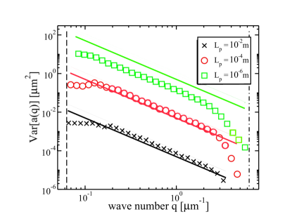
Figure 2: Variance of the amplitudes $a(q)$ for a SFF pulled by thermal linkers (symbols), for various bending rigidities (or, equivalently, various persistence lengths). The straight lines give the purely thermal bending spectra for the same persistence lengths (see Eq. (6)).

In our model, the fluctuations enforced through the active linkers differ strongly from purely thermal fluctuations: First, the fluctuations are transmitted not continuously in space but only at the binding sites of the cross-linkers. Second, the dynamics of active cross-linkers does not fulfill detailed-balance, as discussed previously. In order to disentangle these two effects, we start our analysis with thermal cross-linkers rather than with active ones.

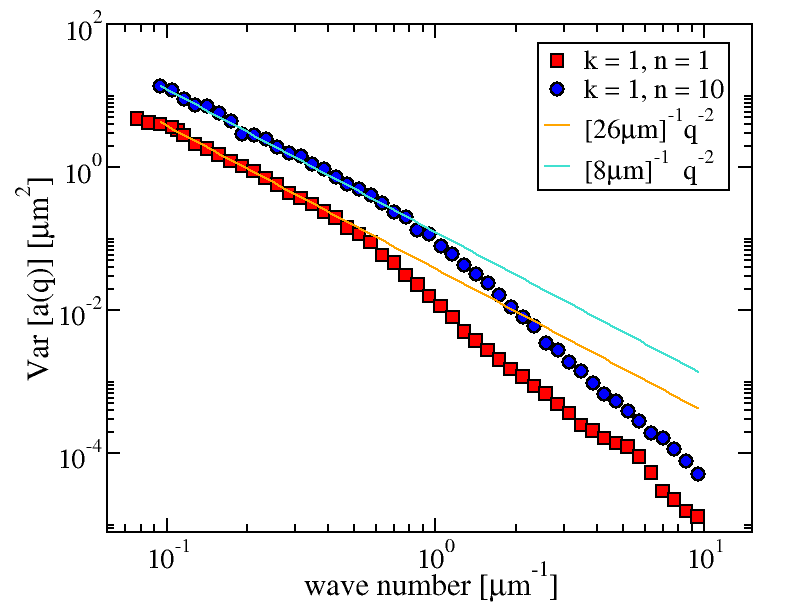
Figure 3: Variance of the amplitudes $a(q)$ for a SFF deformed by active linkers. For the red squares, the parameters are those of Table 1 (SM sm ). The data follow a $q^{-2}$ behavior (orange line) for small $q$, which can be associated with a persistence length of $26\mu$m. However we find a significant deviation from the $q^{-2}$ spectrum for larger wave vectors. An increase by a factor of $n=10$ of both $F_{d}$ and $F_{s}$ (blue circles, stronger motors) extends the $q^{-2}$ regime, but does not suppress the deviation completely.

Thermal cross-linkers – In Fig. 2 we show the cosine bending spectrum for thermal linkers, for three different bending rigidities and compare it to the purely thermal spectrum. For all bending rigidities we observe deviations from the purely thermal spectrum for small values of $q\sim 1/L$. These can be attributed to the finite length of the SFF. Modes for large wavenumbers $q\sim 1/d_{\rm mesh}$ are also suppressed due to the finite distance between neighboring cross-linkers. For intermediate values of $q$ one indeed observes the expected $q^{-2}$ spectrum. As long as the persistence length is at least of the order of the system size, we are in the regime of small deviations and one obtains the expected value of the persistence length. In the context of biological applications it is interesting to notice that the mesh size of the background lattice and the typical length of the SFF determine the range of the $q^{-2}$ spectrum.

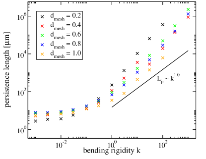
Figure 4: Persistence length as a function of the bending rigidity for various background network mesh size $d_{\rm{mesh}}$ (in $\mu$m) and for active linkers. For comparison, the straight line gives the linear increase expected for purely thermal fluctuations (Eq. 6).

Active cross-linkers – As a second step of our analysis, we now consider model with active cross-linkers. For active cross-linkers one observes generically strong deviations of the bending spectrum from $q^{-2}$ even in the regime $1/L<q<1/d_{\rm mesh}$. The actual form of the spectrum depends strongly on the model parameters. In Fig. 3 we show bending spectra for SFF with $k=1$, i.e. the bending rigidity of microtubules. For this value of $k$ and realistic biological parameters for the linker forces and mesh size, we find a thermal like $q^{-2}$ spectrum for small wave vectors while deviations arise for larger wave numbers. The extension of the $q^{-2}$ regime is even larger if $F_{d}$ and $F_{s}$ are scaled up by a factor of $n=10$, i.e. if linkers are made stronger. Using the $q^{-2}$ part of the bending spectrum we obtain an apparent persistence length of $26\mu m$, surprisingly close to the experimentally obtained value of $30\mu m$ for in vivo microtubule fluctuations Brangwynne et al. (2007b).

As mentioned above, generically we observe rather strong deviations from the $q^{-2}$ regime. Therefore, from now on, the persistence is estimated via the tangent angle correlation (7) to ensure reliable persistence length estimation for all bending rigidities. In the case of purely thermal fluctuations, the persistence length is proportional to the bending rigidity. Fig. 4 reveals that the active linker-driven SFF’s persistent length evolves in a more complex way. For small $k$ we observe only a weak dependency of the apparent SFF stiffness on the bending rigidity, as the deformations are limited by the mesh size. An increase of the bending rigidity to $k\geq 1$ leads to a super-linear increase of the persistence length up to, and beyond the SFF length.

Finally we also studied the effect of varying the mesh size of the underlying network, for various bending rigidities of the SFF and a fixed number of active-linkers. As seen in Fig. 4, for low bending rigidities, the persistence length slightly decreases with $d_{\rm{mesh}}$ (This dependence is linear in $d_{\rm{mesh}}$, as can be seen in Fig. S2 in SM sm ). Though we use here the model beyond the limit of small deformations, we expect this conclusion to hold. Indeed, closer linkers can enforce deformations at smaller scales.

Surprisingly this behavior is inverted for large bending rigidities, where one observes larger persistence lengths for higher densities of active linkers. Indeed, when $d_{\rm{mesh}}$ decreases, the curvature induced by a single linker step is more pronounced. At high bending rigidities, this strong local deformation will result into strong load forces, which most likely the linker will not be able to sustain. Therefore, it is difficult to deform the stiff SFF at all, if the density of cross-linkers is too high.

Discussion– In this paper we have proposed a modeling approach to describe the dynamics of a semi-flexible filament subject to fluctuations generated by a finite set of cross-linkers. For any configuration of the linkers, we are able to compute the equilibrium shape of the semi-flexible filament, using a semi-analytical method, and also to calculate the feedback on the linkers dynamics due to the SFF rigidity. This allows us to study quantitatively the effect of cross-linker induced deformations on the shape of the SFF for various types of linker dynamics.

In this work we considered fluctuations generated by thermal and active linkers, where the dynamics of the latter is based on the dynamics of typical kinesin motors. In both cases linkers step perpendicular to the SFF. For thermal linkers we observe a $q^{-2}$ regime in the bending spectrum, whose range is limited by the length of the SFF for small $q$ and by the distance between two linkers for large $q$.

In the case of active cross-linkers, one observes typically strong deviations from the $q^{-2}$ bending spectrum, as a signature of non-thermal fluctuations, in agreement with experimental observations Brangwynne et al. (2008). For biologically relevant parameters, however, a $q^{-2}$ spectrum has been observed in a certain interval of wave-numbers. Interestingly, using this part of the bending spectrum one obtains an estimate of the persistence length which is very close to the experimental value found in Brangwynne et al. (2007b). This agreement is remarkable, in view of the fact that we only assumed fluctuations perpendicular to the filament and motor based microscopic dynamics.

Regarding the dynamics of the motor-driven SFF, our simulation results show the absence of bidirectional persistent displacement, which could be expected from a tug-of-war scenario Müller et al. (2008). These results are in agreement with explicit transport models Kunwar et al. (2011); Klein et al. (2015).

Our approach can be generalized to other types of non-thermal forcing and boundary conditions and thus could be used in order to describe a large range of experimental settings.

Supplementary Material
Non-equilibrium fluctuations of a semi-flexible filament driven by active cross-linkers

$$p(F_{\rm{SFF}})=\rm{max}\left[0,p_{0}\left(1-\frac{|F_{\rm{SFF}}|}{F_{\rm{s}}}\right)\right].$$ (S1)

On the contrary, stepping rate increases for a load force in the same direction as the stepping

$$p(F_{\rm{SFF}})=\rm{min}\left[2p_{0},p_{0}\left(1+\frac{|F_{\rm{SFF}}|}{F_{\rm{s}}}\right)\right].$$ (S2)

Though our model is an idealized one, we still used some parameters corresponding to biological measurements, as given in the table below. In particular, the linkers’ parameters are close to the kinesin ones. The reference bending rigidity is the experimentally measured value $k=1.10^{-23}$Nm² for microtubules Gittes et al. (1993).

Semi-flexible filament parameters		Value
Bending rigidity in $k_{MT}$ units	$k$	$1\,k_{MT}$
Bending rigidity of microtubules	$k_{MT}$	$1.10^{-23}\,\text{Nm}^{2}$
Background mesh size	$d_{\rm{mesh}}$	$1$ $\mu$m
Filament contour length	$L$	$100$ $\mu$m
Cross linkers parameters		Value
Binding rate	$\omega_{\rm{a}}$	$0.05\,\text{s}^{-1}$
Unbinding rate	$\omega_{\rm{d}_{0}}$	$0.01\,\text{s}^{-1}$
Hopping rate	$p_{0}$	$1\,\text{s}^{-1}$
Detachment force	$F_{\rm{d}}$	3 pN
Stall force	$F_{\rm{s}}$	6 pN
Step size	$\delta$	10 nm
Length of coupling chain	$l_{\rm{max}}$	10 steps

Table 1: System parameters and single active cross-linker characteristics.

I Polynomial description of the semi flexible filament shape: Bending energy and local forces

As stated in the core of the paper, the equilibrium shape of the SFF between two attachment points can be taken under the form of a polymer of degree 3 (see Eq. (3) of the main text), with the boundary conditions given by Eqs. (4) and (5) of the main text. Putting all these polynomials end-to-end to construct the whole SFF, this allows us to determine the polynomial’s coefficients

$$a_{i} = -2\frac{\Delta z_{i}}{\Delta x_{i}^{3}}+\frac{1}{\Delta x_{i}^{2}}\left(2v_{i}+\Delta v_{i}\right)$$ (S3)

$$b_{i} = 3\frac{\Delta z_{i}}{\Delta x_{i}^{2}}-\frac{1}{\Delta x_{i}}\left(3v_{i}+\Delta v_{i}\right)$$ (S4)

$$c_{i} = v_{i}$$ (S5)

$$d_{i} = z_{i}.$$ (S6)

Here $\Delta x_{i}=x_{i+1}-x_{i}$ is the distance of two consecutive pulling cross-linkers, $\Delta z_{i}=z_{i+1}-z_{i}$ their vertical displacement difference and $\Delta v_{i}=v_{i+1}-v_{i}$ the difference of slopes. For simplicity, we admit periodic boundary conditions. The energy of the SFF

$$E=z^{t}\tilde{B}z-v^{t}\Lambda+v^{t}\,\tilde{A}\,v\;,$$ (S7)

where the matrices $\tilde{A}$ and $\tilde{B}$ are given by

$$\tilde{A}_{ij} = 4k\left(\frac{1}{\Delta x_{i}}+\frac{1}{\Delta x_{i-1}}\right),\quad\text{if }i=j$$ (S8)

$$= \frac{2k}{x_{\max(i,j)}-x_{\min(i,j)}},\quad\text{if }i=j\pm 1$$

$$= 0\quad\text{else}$$

and

$$\tilde{B}_{ij} = 12k\left(\frac{1}{\Delta x_{i}^{3}}+\frac{1}{\Delta x_{i-1}^{3}}\right),\quad\text{if }i=j,$$ (S9)

$$= -\frac{12k}{(x_{\max(i,j)}-x_{\min(i,j)})^{3}},\quad\text{if }i=j\pm 1$$

$$= 0\quad\text{else.}$$

while the components of the vector $\Lambda$ in Eq. (S7) are given by

$$\Lambda_{i}=12\,k\,\left[\frac{\Delta z_{i}}{(\Delta x_{i})^{2}}+\frac{\Delta z_{i-1}}{(\Delta x_{i-1})^{2}}\right]\;.$$ (S10)

The gradient $v$ is chosen in such a way that it minimizes the total energy in (S7), which allows us to write

$$\Lambda_{i}=2\sum_{j}\tilde{A}_{ji}v_{j}.$$ (S11)

The coupling matrix for slopes $\tilde{A}$ and for the local displacements $\tilde{B}$ are both cyclic-tridiagonal and take the form With the gradient $v_{i}=\frac{1}{2}\sum_{k}\tilde{A}_{ik}^{-1}\Lambda_{k}$ a simple form for the global SFF energy is

$$E=z^{t}\tilde{B}z-\frac{1}{4}\Lambda^{t}\tilde{A}^{-1}\Lambda$$ (S12)

and the local force reads

$$F_{k}=\frac{\partial E}{\partial z_{k}} = 24k\left(\frac{\Delta z_{k-1}}{\Delta x_{k-1}^{3}}-\frac{\Delta z_{k}}{\Delta x_{k}^{3}}\right)$$ (S13)

$$-12k\left\{v_{k}\left(\frac{1}{\Delta x_{k-1}^{2}}-\frac{1}{\Delta x_{k}^{2}}\right)\right\}$$

$$-12k\left\{\frac{v_{k-1}}{\Delta x_{k-1}^{2}}-\frac{v_{k+1}}{\Delta x_{k}^{2}}\right\}.$$

II Update Algorithm

Let us assume we start in a state for which we know the force applied on each bound cross-linker, and thus all the transition rates (a possible initial state can be a flat SFF with no cross-linker attached).

• We update the system of linkers with a tower sampling algorithm and perform stochastic events until the occurrence of an event that modifies the force exerted on the SFF.

• Then the new equilibrium shape of the SFF is calculated as explained in the next section.

• The new forces exerted on the linkers are obtained and the value of force-dependent rates is calculated for each linker.

This procedure is repeated to update the system.

III No tensibility condition

Though we assume that deformations are small enough to have no overhang in the SFF shape, still deformations can be large enough to change significantly the length of the polymer. As we assume a non tensile polymer, we have to rescale the SFF in order to keep a constant length. When the vertical deformation becomes important, the horizontal extension of the SFF should decrease, and the other way round when the deformation decreases. This is done by removing or adding an empty attachment site at a randomly chosen position. As this is a discrete adjustment, it cannot compensate completely the length change, and a small rescaling in $x$ and $z$ direction is needed to keep the SFF’s contour length constant.

IV Definition of the persistence length

A persistence length gives the typical distance over which a polymer subject to a given type of fluctuations is deformed. The persistence length obviously depends on the fluctuations which are applied. When not stated, these fluctuations are in general implicitly assumed to be purely thermal fluctuations. However, a persistence length can a priori be defined for any kind of fluctuations - including the fluctuations due to cross-linkers as we consider in this paper.

As stated in the main text (Eq. (7)), a general definition of persistence lengths can be given from the two point correlation function of the tangent angle $\theta(s)$.

However, it is important to realize that, even when one considers purely thermal fluctuations, it is important to distinguish two dimensional and three dimensional fluctuations. Indeed, the deformation will not be the same in these two cases. In the literature, one can find two strategies to account for these differences.

• (i) either a unique definition is given in terms of the two point correlation function of the tangent angle $\theta(s)$, but different values of the persistence length will be found for purely thermal fluctuations depending whether these fluctuations are applied in a 2D or 3D space.

• (ii) or a different definition is given depending on the dimension of space, resulting in a unique value of the persistence length for purely thermal fluctuations.

While the first point of view was used for example in Kierfeld et al. (2008), the second one was considered in Gittes et al. (1993); Brangwynne et al. (2007b).

In our paper, we chose to take the point of view (ii). Then the definition of the persistence length for 3D fluctuations is

$$\langle\cos\left(\theta(s)-\theta(s^{\prime})\right)\rangle=\exp\left(-|s-s^{\prime}|/L_{\text{p}}\right),$$ (S14)

while a factor $2$ has to be added in front of $L_{\text{p}}$ when considering two dimensional fluctuations, as given in Eq. (7) of the main text. Then the definition of Eq. (7) is consistent with the one of Eq. (6).

V Deformations under active linkers

In Fig. S1, we show the linear dependence of the persistence length as a function of the background network mesh size $d_{\rm{mesh}}$.

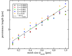
Figure S1: Persistence length as a function of the background network mesh size $d_{\rm{mesh}}$ in the case of active linkers. For flexible SFFs we observe a linear increase of the apparent stiffness with increasing mesh size.