Explosive Phase Transition in a Majority-Vote Model with Inertia

Abstract

We generalize the original majority-vote model by incorporating an inertia into the microscopic dynamics of the spin flipping, where the spin-flip probability of any individual depends not only on the states of its neighbors, but also on its own state. Surprisingly, the order-disorder phase transition is changed from a usual continuous type to a discontinuous or an explosive one when the inertia is above an appropriate level. A central feature of such an explosive transition is a strong hysteresis behavior as noise intensity goes forward and backward. Within the hysteresis region, a disordered phase and two symmetric ordered phases are coexisting and transition rates between these phases are numerically calculated by a rare-event sampling method. A mean-field theory is developed to analytically reveal the property of this phase transition.

Phase transitions in ensembles of complex networked systems have been a subject of intense research in statistical physics and many other disciplines Dorogovtsev et al. (2008). These results are of fundamental importance for understanding various dynamical processes in real world, such as percolation Cohen et al. (2000); Callaway et al. (2000), epidemic spreading Pastor-Satorras et al. (2015), synchronization Arenas et al. (2008); Rodrigues et al. (2016), and collective phenomena in social networks Castellano et al. (2009).

Recently, explosive or discontinuous transitions in complex networks have received growing attention since the discovery of an abrupt percolation transition in random networks Achlioptas et al. (2009); Friedman and Landsberg (2009) and scale-free networks Radicchi and Fortunato (2009); Cho et al. (2009). Later studies affirmed that this transition is actually continuous but with an unusual finite size scaling da Costa et al. (2010); Grassberger et al. (2011); Riordan and Warnke (2011), yet many related models show truly discontinuous and anomalous transitions (cf. Souza and Nalger (2015) for a recent review). Striking different from continuous phase transitions, in an explosive transition an infinitesimal increase of the control parameter can give rise to a considerable macroscopic effect. Subsequently, an explosive phenomenon was found in the dynamics of cascading failures in interdependent networks Buldyrev et al. (2010); Parshani et al. (2010); Gao et al. (2011), in contrast to the second-order continuous phase transition found in isolated networks. More recently, such explosive phase transitions have been reported in various systems, such as explosive synchronization due to a positive correlation between the degrees of nodes and the natural frequencies of the oscillators Gómez-Gardeñes et al. (2011); Leyva et al. (2012); Ji et al. (2013) or an adaptive mechanism Zhang et al. (2015), discontinuous percolation transition due to an inducing effect Zhao et al. (2013), spontaneous recovery Majdandzic et al. (2014), and explosive epidemic outbreak due to cooperative coinfections of multiple diseases Chen et al. (2013); Cai et al. (2015); Hébert-Dufresnea and Althousea (2015).

In this paper we report an explosive order-disorder phase transition in a generalized majority-vote (MV) model by incorporating the effect of individuals’ inertia (called inertial MV model). The MV model is one of the simplest nonequilibrium generalizations of the Ising model that displays a continuous order-disorder phase transition at a critical value of noise de Oliveira (1992). It has been extensively studied in the context of complex networks, including random graphs Pereira and Moreira (2005); Lima et al. (2008), small world networks Campos et al. (2003); Luz and Lima (2007); Stone and McKay (2015), and scale-free networks Lima (2006); Lima and Malarz (2006). However, the continuous nature of the order-disorder phase transition is not affected by the topology of the underlying networks Chen et al. (2015). In our model, we have included a substantial change to make it more realistic, namely the state update of each node depends not only on the states of its neighboring nodes, but also on its own state. In fact, in a social or biological context individuals have a tendency for beliefs to endure once formed. In a recent experimental study, behavioral inertia was found to be essential for collective turning of starling flocks Attanasi et al. (2014). We refer this modification as inertial effect. Surprisingly, we find that as the level of the inertia increases, the nature of the order-disorder phase transition is changed from a continuous second-order transition to a discontinuous, or an explosive, first-order one. For the latter case, a clear hysteresis region appears in which the order and disordered phases are coexisting. In particular, a relevant phenomenon of inertia-induced first-order synchronization transition was found in a second-order Kuramoto model Tanaka et al. (1997); Gupta et al. (2014). A counterintuitive “slower is faster” effect of the inertia on ordering dynamics of the voter model was reported in a recent work Stark et al. (2008).

We first describe the original MV model defined on underlying networks. Each node is assigned to a binary spin variable ${\sigma_{i}}\in\{+1,-1\}$ $(i=1,\ldots,N)$. In each step, a node $i$ is randomly chosen and tends to align with the local neighborhood majority but with a noise parameter $f$ giving the probability of misalignment. In this way, the single spin-flip probability from $\sigma_{i}$ to $-\sigma_{i}$ can be written as

$$w(\sigma_{i})=\frac{1}{2}\left[{1-(1-2f)\sigma_{i}S\left({\Theta_{i}}\right)}\right]$$ (1)

with

$$\Theta_{i}=\sum\limits_{j=1}^{N}a_{ij}\sigma_{j}$$ (2)

where $S(x)=sgn(x)$ if $x\neq 0$ and $S(0)=0$. The elements of the adjacency matrix of the underlying network are defined as $a_{ij}=1$ if nodes $i$ and $j$ are connected and $a_{ij}=0$ otherwise.

In the original MV model, the state update of each node depends exclusively on the states of its neighboring nodes, regardless of its own state. Here, we incorporate the inertial effect into the original model by replacing Eq.(2) with

$$\Theta_{i}=(1-\theta)\sum\limits_{j=1}^{N}a_{ij}\sigma_{j}/k_{i}+\theta\sigma_{i}$$ (3)

where $k_{i}=\sum\nolimits_{j=1}^{N}a_{ij}$ is the degree of node $i$, and $\theta\in[0,0.5]$ is a parameter controlling the weight of the inertia. The larger the value of $\theta$ is, the larger the inertia of the system is. For $\theta=0$, we recover to the original MV model where no inertia exists. For $\theta=0.5$, our model is dominated by the inertia other than the random spin flip with the probability $f$. In this case, there is no spontaneous magnetization to appear. If $\theta=0.5$ and $f=0$, the spins are frozen into the initial configuration. We should note that the generalization of the inertial MV model from two states to multiple states is straightforward, which is discussed in the Supplementary Material SM (1).

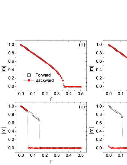
Figure 1: (color online). The absolute magnetization $|m|$ as a function of noise intensity $f$ on ER random networks with different inertia parameter $\theta=0$ (a), $\theta=0.2$ (b), $\theta=0.3$ (c), and $\theta=0.35$ (d). The symbols squares and circles correspond to forward and backward simulations, respectively. The network parameters are $N=10,000$ and $\left\langle k\right\rangle=20$.

The phase behavior of the system can be characterized by the average magnetization per node, $m=\sum\nolimits_{i=1}^{N}\sigma_{i}/N$. $m=0$ for the disordered phase and $m\neq 0$ for the ordered phase. By Monte Carlo (MC) simulations, Fig.1 shows the absolute value of $m$ as a function of $f$ for several different values of $\theta$ on Erdös-Rényi (ER) random networks (ER-RN) with the size $N=10,000$ and the average degree $\left\langle k\right\rangle=20$. The simulation results are obtained by performing forward and backward simulations, respectively. The former is done by calculating the stationary value of $m$ as $f$ increases from 0 to 0.5 in steps of 0.01, and using the final configuration of the last simulation run as the initial condition of the next run, while the latter is performed by decreasing $f$ from 0.5 to 0 with the same step. For $\theta=0$, the results on the forward and backward simulations coincide, implying that the order-disorder transition is a continuous second-order phase transition that is the main feature of the original MV model. For $\theta=0.2$, although the transition becomes sharper and the transition point shifts to a smaller value of $f$, the forward and backward simulations still coincide. Strikingly, for $\theta=0.3$, one can see that as $f$ increases, $|m|$ abruptly jumps from nonzero to zero at $f=f_{c_{F}}$, which shows that a sharp transition takes place for the order-disorder transition (Fig.1(c)). On the other hand, the curve corresponding to the backward simulations also shows a sharp transition from the disordered phase to the order phase at $f=f_{c_{B}}$. These two sharp transitions occur at different values of $f$, leading to a clear hysteresis loop with respect to the dependence of $|m|$ on $f$. Such a feature indicates that a discontinuous first-order order-disorder transition arises due to the effect of inertia. Further increasing $\theta$ to $\theta=0.35$, $f_{c_{F}}$ shifts to a smaller value and $f_{c_{B}}$ decreases to zero, but the nature of a discontinuous phase transition is still present.

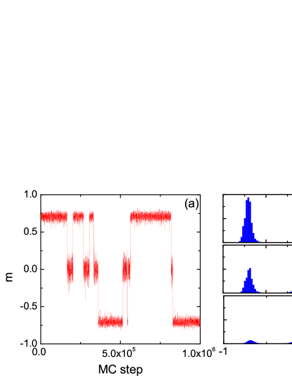
Figure 2: (color online). (a) Time series of magnetization $m$ show the transition events between ordered and disordered phases within the hysteresis region. (b-d) show the PDF of $m$ for $f=0.136$ (b), $f=0.138$ (c), and $f=0.14$ (d). The other parameters are $\theta=0.3$, $N=500$, and $\left\langle k\right\rangle=20$.

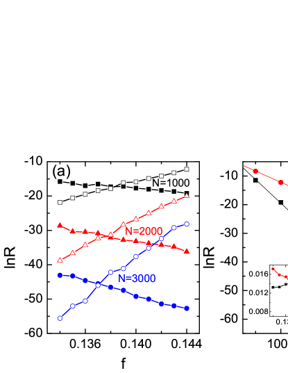
Figure 3: (color online). (a) The logarithm of transition rates $\ln R$ as a function of $f$ for different $N$. Solid symbols correspond to the transition rate from disordered state to ordered state, and empty symbols to the transition rate from ordered state to disordered state. (b) $\ln R$ as a function of $N$ for $f=0.144$. The lines indicate the linear fitting $\ln R_{1(2)}\sim-\nu_{1(2)}N$. The inset shows the fitting exponents $\nu_{1(2)}$ as a function of $f$.

Within the hysteresis region, we observe phase flips between the ordered phase and the disordered one for a rather small network size $N$, as shown in Fig.2(a) by a long time series of $m$ in a ER network of $N=500$. We show in Fig.2(b-d) the probability density function (PDF) of $m$ for three distinct $f$ chosen from the hysteresis region. On the one hand, all of them are multimodal distributions with a peak at $m=0$ and two other peaks symmetrically located at both sides of it. On the other hand, with the increase of $f$ the peak at $m=0$ becomes higher implying that the disorder phase becomes more stable. To calculate the transition rates between the ordered and disordered phases, a long-time simulation is necessary. However, for a larger network size the transition rates are extremely low and brute-force simulation is prohibitively expensive. To overcome this difficulty, we have used a recently developed rare-event simulation method, the forward flux sampling (FFS) Allen et al. (2005, 2009). In Fig.3(a), we show the transition rates $R_{1}$ from disordered to ordered phases and the inverse transition rate $R_{2}$ as a function of $f$ for several different $N$. $R_{1}$ is a deceasing function of $f$ and $R_{2}$ is an increasing function of $f$. The intersection point of both curves determines the location at which the ordered and the disordered phase are equally stable. As $N$ increases, the intersection point slightly shifts to a smaller value. In Fig.3(b), we show the transition rates as a function of $N$ at $f=0.144$. Obviously, both $R_{1}$ and $R_{2}$ decrease exponentially with $N$, $R_{1(2)}\sim\exp\left(-\nu_{1(2)}N\right)$ with the exponents $\nu_{1(2)}$, implying that the disordered and ordered phases are coexisting in the thermodynamic limit. In the inset of Fig.3(b), we give the fitting exponents $\nu_{1(2)}$ as a function of $f$, and they clearly exhibit the different variation trends with $f$.

In the following, we will present a mean-field theory to understand the simulation results. We first define $m_{k}$ as the average magnetization of a node of degree $k$, and $\tilde{m}$ as the average magnetization of a randomly chosen nearest-neighbor node. For uncorrelated networks, the probability that a randomly chosen nearest-neighbor node has degree $k$ is $kP(k)/\left\langle k\right\rangle$, where $P(k)$ is the degree distribution defined as the probability that a node chosen at random has degree $k$ and $\left\langle k\right\rangle$ is the average degree Dorogovtsev et al. (2008). Thus, $m_{k}$ and $\tilde{m}$ satisfy the following relation

$$\tilde{m}=\sum\limits_{k}kP(k)m_{k}/\left\langle k\right\rangle.$$ (4)

For an up-spin node $i$ of degree $k$, the probability that its local field is positive can be written as the cumulative binomial distribution,

$$P_{>}^{+}=\sum\limits_{n=\left\lceil{n_{k}^{+}}\right\rceil}^{k}{\left({1-\frac{1}{2}{\delta_{n,n_{k}^{+}}}}\right)}C_{k}^{n}{p_{\uparrow}^{n}}{p_{\downarrow}^{k-n}}.$$ (5)

Here, $p_{\uparrow(\downarrow)}=(1\pm\tilde{m})/2$ is the probability that a randomly chosen nearest-neighbor node has $+1$ ($-1$) state, $\left\lceil\cdot\right\rceil$ is the ceiling function, $\delta$ is the Kronecker symbol, $C_{k}^{n}=k!/[n!(k-n)!]$ are the binomial coefficients, and $n_{k}^{+}=(1-2\theta)k/[2(1-\theta)]$ is the number of up-spin neighbors of node $i$ satisfying $\Theta_{i}=0$. Similarly, we can write the probability that the local field of a down-spin node of degree $k$ is positive as,

$$P_{>}^{-}=\sum\limits_{n=\left\lceil{n_{k}^{-}}\right\rceil}^{k}{\left({1-\frac{1}{2}{\delta_{n,n_{k}^{-}}}}\right)}C_{k}^{n}{p_{\uparrow}^{n}}{p_{\downarrow}^{k-n}},$$ (6)

where $n_{k}^{-}=k-n_{k}^{+}=k/[2(1-\theta)]$.

Furthermore, the spin-flip probability $\omega_{k}^{+}$ of an up-spin node of degree $k$ can be expressed as the sum of two parts.

$$\omega_{k}^{+}=fP_{>}^{+}+(1-f)(1-P_{>}^{+}),$$ (7)

where the first part is that the local field of the node is positive and the minority rule is applied, and the other one is that the local field of the node is negative and the majority rule is applied. Likewise, we can write the spin-flip probability of a down-spin node of degree $k$ as,

$$\omega_{k}^{-}=f(1-P_{>}^{-})+(1-f)P_{>}^{-}$$ (8)

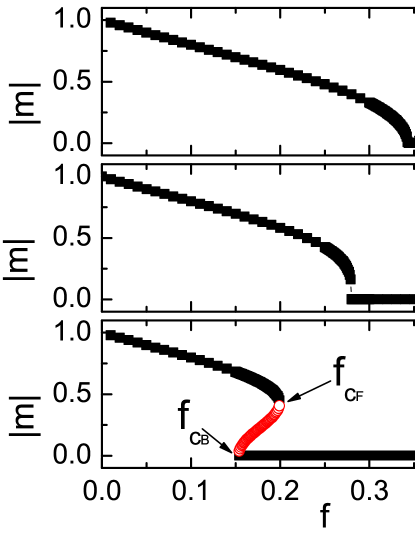
Figure 4: (color online). Theoretical result of $|m|$ as a function of $f$ for three typical values of $\theta$: (a) $\theta=0.15$, (b) $\theta=0.23$, and (c) $\theta=0.3$. In Fig.4(c), circles within the hysteresis region indicate the unstable solution.

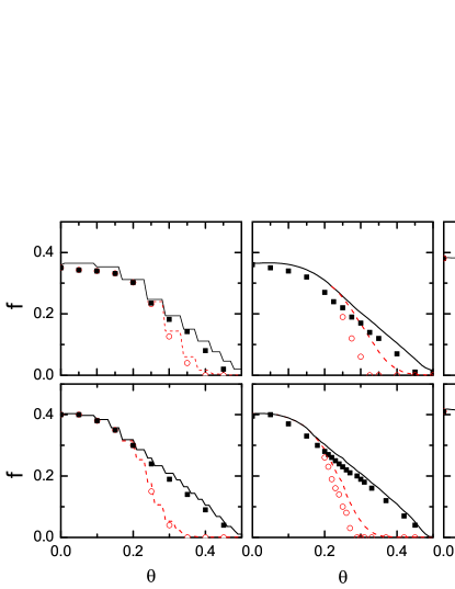
Figure 5: (color online). Phase diagram in the $\theta-f$ plane for three types of networks with two different average degree: $\left\langle k\right\rangle=20$ (top panels) and $\left\langle k\right\rangle=40$ (bottom panels). For left to right: Rd-RN, ER-RN, and BA-SFN. Lines and symbols correspond to the theoretical and simulation results, respectively. $f_{c_{F}}$ are indicated by solid lines and squares, and $f_{c_{B}}$ by dashed lines and circles. The sizes of all the networks are the same: $N=10,000$.

Thus, the rate equations for $m_{k}$ are

$$\dot{m}_{k}=-\left({\frac{1+m_{k}}{2}}\right)\omega_{k}^{+}+\left({\frac{1-m_{k}}{2}}\right)\omega_{k}^{-}$$ (9)

In the steady state $\dot{m}_{k}=0$, we have

$$m_{k}=\frac{\omega_{k}^{-}-\omega_{k}^{+}}{\omega_{k}^{+}+\omega_{k}^{-}}$$ (10)

Inserting Eq.(10) into Eq.(4), we get a self-consistent equation of $\tilde{m}$,

$$\tilde{m}=\Psi(\tilde{m}),$$ (11)

with

$$\Psi(\tilde{m})=\sum\limits_{k}{\frac{{kP(k)}}{{\left\langle k\right\rangle}}\frac{{\omega_{k}^{-}-\omega_{k}^{+}}}{{\omega_{k}^{+}+\omega_{k}^{-}}}}.$$

Since $P_{>}^{+}+P_{>}^{-}=1$ and $\omega_{k}^{+}=\omega_{k}^{-}$ at $\tilde{m}=0$, one can easily check that $\tilde{m}=0$ is always a stationary solution of Eq.(11). This solution corresponds to a disordered phase. The other possible solutions can be obtained by numerically iterating Eq.(11). Once $\tilde{m}$ is found, we can immediately calculate $m_{k}$ by Eq.(10) and the average magnetization per node by $m=\sum\nolimits_{k}{P(k)m_{k}}$.

By a detailed numerical calculation for Eq.(11) on ER-RN with the Poisson degree distribution $P(k)=\left\langle k\right\rangle^{k}e^{-\left\langle k\right\rangle}/k!$ and the average degree $\left\langle k\right\rangle=20$, we find that the critical value of $\theta$ is $\theta_{c}=0.23$. In Fig.4, we show the theoretical results on $|m|$ as a function of $f$ for three typical values of $\theta=0.15$, 0.23, and 0.3. For $\theta<\theta_{c}$, the order-disordered phase transition is of continuous second-order type. For $\theta>\theta_{c}$, the phase transition is of discontinuous first-order type and a clear hysteresis loop appears. At $\theta=\theta_{c}$, the order parameter $|m|$ has still a jump at $f=f_{c}$ but no hysteresis loop exists.

At the critical noises, $f_{c_{F}}$ and $f_{c_{B}}$, the susceptibilities $\tilde{\chi}=\partial\tilde{m}/\partial f$ are diverging. According to Eq.(11), the condition is equivalent to

$$\frac{{\partial\Psi}}{{\partial\tilde{m}}} = (1-2f)\sum\limits_{k}{\frac{{kP(k)}}{{\left\langle k\right\rangle}}}[{(\omega_{k}^{-}+\omega_{k}^{+})^{-1}}(\frac{{\partial P_{>}^{+}}}{{\partial\tilde{m}}}+\frac{{\partial P_{>}^{-}}}{{\partial\tilde{m}}})$$ (12)

$$+ (\omega_{k}^{-}-\omega_{k}^{+}){(\omega_{k}^{-}+\omega_{k}^{+})^{-2}}(\frac{{\partial P_{>}^{+}}}{{\partial\tilde{m}}}-\frac{{\partial P_{>}^{-}}}{{\partial\tilde{m}}})]=1$$

Here, $\partial P_{>}^{\pm}/\partial\tilde{m}$ can be derived from Eq.(5) and Eq.(6)

$$\frac{{\partial P_{>}^{\pm}}}{{\partial\tilde{m}}}=\left({1-\frac{1}{2}{\delta_{n_{k}^{\pm},\left\lceil{n_{k}^{\pm}}\right\rceil}}}\right)\mathbb{P}\left({\left\lceil{n_{k}^{\pm}}\right\rceil};k\right)$$

$$+\frac{1}{2}{\delta_{n_{k}^{\pm},\left\lceil{n_{k}^{\pm}}\right\rceil}}\mathbb{P}\left({\left\lceil{n_{k}^{\pm}}\right\rceil+1};k\right),$$ (13)

where the function $\mathbb{P}(n;k)$ is defined as

$$\mathbb{P}(n;k)=\frac{1}{2}kC_{k-1}^{n-1}p_{\uparrow}^{n-1}p_{\downarrow}^{k-n}$$ (14)

For any given $\theta$, $f_{c_{F}}$ and $f_{c_{B}}$ are determined by numerically solving Eqs.(11-12). In fact, $f_{c_{B}}$ can be obtained more conveniently, since $f_{c_{B}}$ corresponds to the point at which the trivial solution $\tilde{m}=0$ loses its stability. Therefore, $f_{c_{B}}$ is determined solely by Eq.(12). At $\tilde{m}=0$, Eq.(12) can be reduced to

$${\left.{\frac{{\partial\Psi}}{{\partial\tilde{m}}}}\right|_{\tilde{m}=0}}=(1-2{f_{c_{B}}}){\sum\limits_{k}{\frac{{kP(k)}}{{\left\langle k\right\rangle}}\left[{\frac{{\frac{{\partial P_{>}^{+}}}{{\partial\tilde{m}}}+\frac{{\partial P_{>}^{-}}}{{\partial\tilde{m}}}}}{{\omega_{k}^{-}+\omega_{k}^{+}}}}\right]}_{\tilde{m}=0}}=1$$ (15)

In Fig.5 we plot the phase diagram in the $\theta-f$ plane for three types of networks (from left to right: random degree-regular networks (Rd-RN), ER-RN, and Barabási-Albert scale-free networks (BA-SFN)) with two different average degrees: $\left\langle k\right\rangle=20$ (top panels) and $\left\langle k\right\rangle=40$ (bottom panels). The lines and symbols indicate the theoretical and simulation results, respectively. For Rd-RN, each node has the same degree $k$, which is a typical representation of degree homogeneous networks. For BA-SFN, its degree distribution follows a power-law function with the exponent $-3$, which is typical for degree heterogeneous networks. Clearly, there is no essential difference in the phase diagrams for different network types and average degree. The phase diagram is divided into three regions by $f_{c_{F}}$ and $f_{c_{B}}$. In the region below $f_{c_{B}}$, the system is ordered. In the region above $f_{c_{F}}$, the system is disordered. Between $f_{c_{F}}$ and $f_{c_{B}}$, the region is of hysteresis with a disordered phase and two ordered phases of up-down symmetry. As expected, for networks with a larger average degree the mean-field theory provides a better prediction for the simulation results. Although there exists obvious differences for a smaller network connectivity, the theory and simulations are qualitatively consistent.

In conclusion, we have investigated the order-disorder phase transition in a MV model with inertia, where the inertia is introduced into the state-updating dynamics of nodes by considering the state of each node itself besides the states of its neighboring nodes. We mainly find that in contrast to a continuous second-order phase transition in the original MV model, the inertial MV model undergoes a discontinuous first-order phase transition when the inertia is large enough. In the hysteresis region of the first-order phase transition, a disordered phase and two symmetric ordered phases are coexisting. The transition rates between the disordered and ordered phases have been calculated by FFS sampling. A mean-field theory provides an analytical understanding for this interesting phenomenon. Since behavioral inertia is an essential characteristic of human being and animal groups, our work may shed a novel understanding of transition phenomena from disorder to order, like the emergence of consensus and decision-making Sood and Redner (2005); Hartnett et al. (2016), as well as the spontaneous formation of a common language/culture Castellano et al. (2009, 2000). Finally, we expect further investigations of inertial effect in other dynamical systems.