Projective method of multipliers for linearly constrained convex minimization

Abstract.

We present a method for solving linearly constrained convex optimization problems, which is based on the application of known algorithms for finding zeros of the sum of two monotone operators (presented by Eckstein and Svaiter) to the dual problem. We establish convergence rates for the new method, and we present applications to TV denoising and compressed sensing problems.

1. Introduction

A broad class of problems of recent interest in image science and signal processing can be posed in the framework of convex optimization. Examples include the TV denoising model [23] for image processing and basis pursuit, which is well known for playing a central role in the theory of compressed sensing. A general subclass of such programming problems is:

(1) $$\begin{split}\min_{u\in\mathbb{R}^{m_{1}},v\in\mathbb{R}^{m_{2}}}\left\{f(u)+g(v)\,:\,Mu+Cv=d\right\}.\end{split}$$

Here $f:\mathbb{R}^{m_{1}}\rightarrow(-\infty,\infty]$ and $g:\mathbb{R}^{m_{2}}\rightarrow(-\infty,\infty]$ are proper closed convex functions, $M:\mathbb{R}^{m_{1}}\rightarrow\mathbb{R}^{n}$ and $C:\mathbb{R}^{m_{2}}\rightarrow\mathbb{R}^{n}$ are linear operators, and $d\in\mathbb{R}^{n}$.

A well-known iterative method for solving optimization problems that have a separable structure as (1) does, is the Alternating Direction Method of Multipliers (ADMM), which goes back to the works of Glowinski and Marrocco [12], and of Gabay and Mercier [11]. ADMM solves the coupled problem (1) performing a sequences of steps that decouple functions $f$ and $g$, making it possible to exploit the individual structure of these functions. It can be interpreted in terms of alternating minimization, with respect to $u$ and $v$, of the augmented Lagrangian function associated with problem (1). ADMM can also be viewed as an instance of the method called Douglas-Rachford splitting applied to the dual problem of (1), as was shown by Gabay in [10].

Other splitting schemes have been effectively applied to the dual problem of (1), which is a special case of the problem of finding a zero of the sum of two maximal monotone operators. For example, the Proximal Forward Backward splitting method, developed by Lions and Mercier [16], and Passty [20], corresponds to the well-known Tseng’s [24] Alternating Minimization Algorithm (AMA) for solving (1). This method has simpler steps than ADMM, in the former one of the minimizations of the augmented Lagrangian is replaced by the minimization of the Lagrangian itself; however, it requires strong convexity of one of the objective functions.

The goal of our work is to construct an optimization scheme for solving (1) applying a splitting method to its dual problem. Specifically we are interested in the family of splitting-projective methods proposed in [7] by Eckstein and Svaiter to address inclusion problems given by the sum of two maximal monotone operators. We will apply a specific instance of these algorithms to solve a reformulation of the dual problem of (1) as the problem of finding a zero of the sum of two maximal monotone operators, which allows us to obtain a new algorithm for solving this problem. This iterative method will be referred to as the Projective Method of Multipliers (PMM). The convergence properties of the PMM will be obtained using the convergence results already established in [7]. In contrast to [7], which only studies the global convergence of the family of splitting-projective methods, we also establish in this work the iteration complexity of the PMM. Using the Karush-Kuhn-Tucker (KKT) conditions for problem (1) we give convergence rate for the PMM measured by the pointwise and ergodic iteration-complexities.

The remainder of this paper is organized as follows. Section 2 reviews some definitions and facts on convex functions that will be used in our subsequent presentation. It also briefly discusses Lagrangian duality theory for convex optimization, for more details in this subject we refer the reader to [21]. Section 3 presents the Projective Method of Multipliers (PMM) for solving the class of linearly constrained optimization problems (1). This section also presents global convergence of the PMM using the convergence analysis presented in [7]. Section 4 derives iteration-complexity results for the PMM. Finally, section 5 presents some applications in image restoration and compressed sensing. This section also exhibits numerical results demonstrating the effectiveness of the PMM in solving these problems.

1.1. Notation

Throughout this paper, we let $\mathbb{R}^{n}$ denote an $n$-dimensional space with inner product and induced norm denoted by $\left\langle\cdot,\cdot\right\rangle$ and $\left\|\cdot\right\|$, respectively. For a matrix $A$, $A^{T}$ indicates its transpose and $\left\|A\right\|_{F}=\sqrt{trace(AA^{T})}$ its Frobenius norm. Given a linear operator $M$, we denote by $M^{\ast}$ its adjoint operator. If $C$ is a convex set we indicate by $\textnormal{ri}\left(C\right)$ its relative interior.

2. Preliminaries

In this section we describe some basic definitions and facts on convex analysis that will be needed along this work. We also discuss the Lagrangian formulation and dual problem of (1). This approach will play an important role in the design of the PMM for problem (1).

2.1. Generalities on convex functions

Given an extended real valued convex function $f:\mathbb{R}^{n}\rightarrow(-\infty,\infty]$, the domain of $f$ is the set

$$\textnormal{dom}\,f=\left\{x\in\mathbb{R}^{n}\,:\,f(x)<\infty\right\}.$$

Since $f$ is a convex function, it is obvious that $\textnormal{dom}\,f$ is convex. We say that function $f$ is proper if $\textnormal{dom}\,f\neq\emptyset$. Furthermore, we say that $f$ is closed if it is a lower semicontinuous function.

Definition 1.

Given a convex function $f:\mathbb{R}^{n}\rightarrow(-\infty,\infty]$ a vector $v\in\mathbb{R}^{n}$ is called a subgradient of $f$ at $x\in\mathbb{R}^{n}$ if

$$f(x^{\prime})\geq f(x)+\left\langle v,x^{\prime}-x\right\rangle\qquad\qquad\forall x^{\prime}\in\mathbb{R}^{n}.$$

The set of all subgradients of $f$ at $x$ is denoted by $\partial f(x)$. The operator $\partial f$, which maps each $x$ to $\partial f(x)$, is called the subdifferential map associated with $f$.

It can be seen immediately from the definition that $x^{\ast}$ is a global minimizer of $f$ in $\mathbb{R}^{n}$ if and only if $0\in\partial f(x^{\ast})$. If $f$ is differentiable at $x$, then $\partial f(x)$ is the singleton set $\{\nabla f(x)\}$.

The subdifferential mapping of a convex function $f$ has the following monotonicity property: for any $x$, $x^{\prime}$, $v$ and $v^{\prime}\in\mathbb{R}^{n}$ such that $v\in\partial f(x)$ and $v^{\prime}\in\partial f(x^{\prime})$, it follows that

(2) $$\left\langle x-x^{\prime},v-v^{\prime}\right\rangle\geq 0.$$

In addition, if $f$ is a proper closed convex function, then $\partial f$ is a maximal monotone operator [22]. This is to say that if $x,\,v\in\mathbb{R}^{n}$ are such that inequality (2) holds for all $x^{\prime}\in\mathbb{R}^{n}$ and $v^{\prime}\in\partial f(x^{\prime})$, then $x\in\textnormal{dom}\,f$ and $v\in\partial f(x)$.

Given $\lambda>0$, the resolvent mapping (or proximal mapping) [19] associated with $\partial f$ is defined as

$$(I+\lambda\partial f)^{-1}(z):=\arg\min_{x\in\mathbb{R}^{n}}\lambda f(x)+\frac{1}{2}\left\|x-z\right\|^{2},\qquad\qquad\forall z\in\mathbb{R}^{n}.$$

The fact that $(I+\lambda\partial f)^{-1}$ is an everywhere well defined function, if $f$ is proper, closed and convex, is a consequence of a fundamental result due to Minty [17]. For example, if $f(x)=\mu\left\|x\right\|_{1}=\mu\sum|x_{i}|$ where $\mu>0$, then

$$(I+\partial f)^{-1}(z)=\textbf{shrink}(z,\mu),$$

where

(3) $$\textbf{shrink}(z,\mu)_{i}:=\max\{|z_{i}|-\mu,0\}sign(z_{i}).$$

The Fenchel-Legendre conjugate of a convex function $f$, denoted by $f^{\ast}:\mathbb{R}^{n}\rightarrow(-\infty,\infty]$, is defined as

$$f^{\ast}(v)=\sup_{x\in\mathbb{R}^{n}}\left\langle v,x\right\rangle-f(x)\,,\qquad\qquad\forall v\in\mathbb{R}^{n}.$$

It is simple to see that $f^{\ast}$ is a convex closed function. Furthermore, if $f$ is proper, closed and convex, then $f^{\ast}$ is a proper function [1].

Definition 2.

Given any convex function $f:\mathbb{R}^{n}\to(-\infty,\infty]$ and $\epsilon\geq 0$, a vector $v\in\mathbb{R}^{n}$ is called an $\epsilon$-subgradient of $f$ at $x\in\mathbb{R}^{n}$ if

$$f(x^{\prime})\geq f(x)+\left\langle v,x^{\prime}-x\right\rangle-\epsilon\qquad\qquad\forall x^{\prime}\in\mathbb{R}^{n}.$$

The set of all $\epsilon$-subgradients of $f$ at $x$ is denoted by $\partial_{\epsilon}f(x)$, and $\partial_{\epsilon}f$ is called the $\epsilon$-subdifferential mapping.

It is trivial to verify that $\partial_{0}f(x)=\partial f(x)$, and $\partial f(x)\subseteq\partial_{\epsilon}f(x)$ for every $x\in\mathbb{R}^{n}$ and $\epsilon\geq 0$. The proposition below lists some useful properties of the $\epsilon$-subdifferential that will be needed in our presentation.

Proposition 2.1.

If $f:\mathbb{R}^{n}\to(-\infty,\infty]$ is a proper closed convex function, $g:\mathbb{R}^{n}\to\mathbb{R}$ is a convex differentiable function in $\mathbb{R}^{n}$, and $M:\mathbb{R}^{m}\to\mathbb{R}^{n}$ is a linear transformation, then the following statements hold:

• $v\in\partial_{\epsilon}f(x)$ if and only if $x\in\partial_{\epsilon}f^{\ast}(v)$ for all $\epsilon\geq 0$;

• $\partial(f+g)(x)=\partial f(x)+\nabla g(x)$ for all $x\in\mathbb{R}^{n}$;

• $\partial(f\circ M)(x)\supseteq M^{\ast}\partial f(Mx)$ for all $x\in\mathbb{R}^{m}$. In addition, if $\textnormal{ri}\left(\textnormal{dom}\,f\right)\cap\textnormal{range}\,M\neq\emptyset$, then $\partial(f\circ M)(x)=M^{\ast}\partial f(Mx)$ for every $x\in\mathbb{R}^{m}$;

• if $x_{i},v_{i}\in\mathbb{R}^{n}$ and $\epsilon_{i},\alpha_{i}\in\mathbb{R}_{+}$, for $i=1,\ldots,k$, are such that

  $$v_{i}\in\partial_{\epsilon_{i}}f(x_{i}),\quad i=1,\ldots,k,\qquad\qquad\sum_{i=1}^{k}\alpha_{i}=1,$$

  and we define

  $$\overline{x}=\sum_{i=1}^{k}\alpha_{i}x_{i},\qquad\quad\overline{v}=\sum_{i=1}^{k}\alpha_{i}v_{i},\qquad\quad\overline{\epsilon}=\sum_{i=1}^{k}\alpha_{i}(\epsilon_{i}+\left\langle x_{i}-\overline{x},v_{i}\right\rangle);$$

  then, we have $\overline{\epsilon}\geq 0$ and $\overline{v}\in\partial_{\overline{\epsilon}}f(\overline{x})$.

Proof.

Statements (a)-(c) are classical results which can be found, for example, in [15] and [21]. For a proof of item (d) see [2] and references therein. ∎

2.2. Lagrangian duality

The Lagrangian function $L:\mathbb{R}^{m_{1}}\times\mathbb{R}^{m_{2}}\times\mathbb{R}^{n}\rightarrow(-\infty,\infty]$ for problem (1) is defined as

(4) $$L(u,v,z)=f(u)+g(v)+\left\langle Mu+Cv-d,z\right\rangle.$$

The dual function is the concave function $\varphi:\mathbb{R}^{n}\to[-\infty,\infty)$ defined by

$$\begin{split}\varphi(z)&=\inf_{(u,v)\in\mathbb{R}^{m_{1}}\times\mathbb{R}^{m_{2}}}L(u,v,z),\end{split}$$

and the dual problem to (1) is

(5) $$\max_{z\in\mathbb{R}^{n}}\varphi(z).$$

Problem (1) will be called the primal problem. Straightforward calculations show that weak duality holds, i.e. $\varphi^{\ast}\leq p^{\ast}$, where $p^{\ast}$ and $\varphi^{\ast}$ are the optimal values of (1) and (5), respectively.

A vector $(u^{\ast},v^{\ast},z^{\ast})$ such that $L(u^{\ast},v^{\ast},z^{\ast})$ is finite and it satisfies

(6) $$\min_{(u,v)\in\mathbb{R}^{m_{1}}\times\mathbb{R}^{m_{2}}}L(u,v,z^{\ast})=L(u^{\ast},v^{\ast},z^{\ast})=\max_{z\in\mathbb{R}^{n}}L(u^{\ast},v^{\ast},z)$$

is called a saddle point of the Lagrangian function $L$. Finding optimal solutions of problems (1) and (5) is equivalent to finding saddle points of $L$ (see [21]). That is, $(u^{\ast},v^{\ast})$ is an optimal primal solution and $z^{\ast}$ is an optimal dual solution if and only if $(u^{\ast},v^{\ast},z^{\ast})$ is a saddle point. Furthermore, if a saddle point of $L$ exists then $p^{\ast}=\varphi^{\ast}$, i.e. there is no duality gap [21].

Notice that, if $(u^{\ast},v^{\ast},z^{\ast})$ is a saddle point, from the definition of $L$ in (4) and equalities (6) we deduce that

$$f(u)+g(v)+\left\langle Mu+Cv-d,z^{\ast}\right\rangle\geq L(u^{\ast},v^{\ast},z^{\ast})\geq f(u^{\ast})+g(v^{\ast})+\left\langle Mu^{\ast}+Cv^{\ast}-d,z\right\rangle$$

for all $u\in\mathbb{R}^{m_{1}}$, $v\in\mathbb{R}^{m_{2}}$, $z\in\mathbb{R}^{n}$. From these relations we can directly derive the Karush-Kuhn-Tucker (KKT) conditions

(7) $$\begin{split}&0=Mu^{\ast}+Cv^{\ast}-d,\\ &0\in\partial f(u^{\ast})+M^{\ast}z^{\ast},\\ &0\in\partial g(v^{\ast})+C^{\ast}z^{\ast},\end{split}$$

which describe an optimal solution of problem (1). Observe that the equality in (7) implies that the primal variables $(u^{\ast},v^{\ast})$ must be feasible. The inclusions in (7) are known as the dual feasibility conditions. We also have that the KKT conditions hold if and only if $(u^{\ast},v^{\ast},z^{\ast})$ is a saddle point of $L$.

Observe that the dual function $\varphi$ can be written in terms of the Fenchel-Legendre conjugates of the functions $f$ and $g$. Specifically,

$$\varphi(z)= \inf_{(u,v)\in\mathbb{R}^{m_{1}}\times\mathbb{R}^{m_{2}}}f(u)+g(v)+\left\langle Mu+Cv-d,z\right\rangle$$

$$= \inf_{u\in\mathbb{R}^{m_{1}}}f(u)+\left\langle Mu,z\right\rangle+\inf_{v\in\mathbb{R}^{m_{2}}}g(v)+\left\langle Cv,z\right\rangle-\left\langle d,z\right\rangle$$

$$= -f^{\ast}(-M^{\ast}z)-g^{\ast}(-C^{\ast}z)-\left\langle d,z\right\rangle.$$

Hence, if we define the functions $h_{1}(z)=\left(f^{\ast}\circ-M^{\ast}\right)(z)$ and $h_{2}(z)=\left(g^{\ast}\circ-C^{\ast}\right)(z)+\left\langle d,z\right\rangle$, we have that the dual problem (5) is equivalent to minimizing $h_{1}+h_{2}$ over $\mathbb{R}^{n}$. Furthermore, since $f^{\ast}$ and $g^{\ast}$ are convex and closed, and $M^{\ast}$ and $C^{\ast}$ are linear operators, it follows that $h_{1}$ and $h_{2}$ are convex closed functions [21]. Therefore, $z^{\ast}$ is a solution of (5) if and only if

(8) $$0\in\partial(h_{1}+h_{2})(z^{\ast}).$$

Throughout this work, we assume that

1. there exists $(u^{\ast},v^{\ast},z^{\ast})$ a saddle point of $L$.

Since condition A.1 implies that the KKT conditions hold, we have from the first inclusion in (7) and Proposition 2.1(a),(c) that $z^{\ast}\in\textnormal{dom}\,(f^{\ast}\circ-M^{\ast})$, which implies that $h_{1}$ is a proper function. A similar argument shows that $h_{2}$ is also a proper function. Therefore, under hypothesis A.1, we have that the subdifferentials $\partial h_{1}$ and $\partial h_{2}$ are maximal monotone operators.

3. The Projective Method of Multipliers

Our proposal in this work is to apply the splitting-projective methods developed in [7], by Eckstein and Svaiter, to find a solution of problem

$$0\in\partial h_{1}(z)+\partial h_{2}(z),$$

and as a consequence a solution of the dual problem (5), since the following inclusion holds

$$\partial h_{1}(z)+\partial h_{2}(z)\subseteq\partial(h_{1}+h_{2})(z)\qquad\quad\forall z\in\mathbb{R}^{n}$$

(see equation (8) and the comments above).

The framework presented in [7] reformulates the problem of finding a zero of the sum of two maximal monotone operators in terms of a convex feasibility problem, which is defined by a certain closed convex “extended” solution set. To solve the feasibility problem, the authors introduced successive projection algorithms that use, on each iteration, independent calculations involving each operator.

Specifically, if we consider the subdifferential mappings $\partial h_{1}$ and $\partial h_{2}$, then the associated extended solution set, defined as in [7], is

(9) $$S_{e}(\partial h_{1},\partial h_{2}):=\left\{(z,w)\in\mathbb{R}^{n}\times\mathbb{R}^{n}\,:\,-w\in\partial h_{1}(z)\,,\,w\in\partial h_{2}(z)\right\}.$$

Since $\partial h_{1}$ and $\partial h_{2}$ are maximal monotone operators it can be proven that $S_{e}(\partial h_{1},\partial h_{2})$ is a closed convex set in $\mathbb{R}^{n}\times\mathbb{R}^{n}$, see [7]. It is also easy to verify that if $(z^{\ast},w^{\ast})$ is a point in $S_{e}(\partial h_{1},\partial h_{2})$ then $z^{\ast}$ satisfies inclusion (8) and consequently it is a solution of the dual problem. Furthermore, the following lemma holds.

Lemma 3.1.

If $(u^{\ast},v^{\ast},z^{\ast})$ is a saddle point of $L$, then

$$(z^{\ast},d-Cv^{\ast})\in S_{e}\left(\partial h_{1},\partial h_{2}\right).$$

Moreover, if we assume the following conditions

1. $\textnormal{ri}\left(\textnormal{dom}\,f^{\ast}\right)\cap\textnormal{range}\,M^{\ast}\neq\emptyset$;

2. $\textnormal{ri}\left(\textnormal{dom}\,g^{\ast}\right)\cap\textnormal{range}\,C^{\ast}\neq\emptyset$.

Then, for all $(z^{\ast},w^{\ast})\in S_{e}(\partial h_{1},\partial h_{2})$ there exist $u^{\ast},v^{\ast}\in\mathbb{R}^{n}$ such that $w^{\ast}=d-Cv^{\ast}$, $w^{\ast}=Mu^{\ast}$ and $(u^{\ast},v^{\ast},z^{\ast})$ is a saddle point of the Lagrangian function $L$.

Proof.

If $(u^{\ast},v^{\ast},z^{\ast})$ is a saddle point of the Lagrangian function, then the KKT optimality conditions hold, and the inclusions in (7), together with Proposition 2.1(a), imply that

$$u^{\ast}\in\partial f^{\ast}(-M^{\ast}z^{\ast})\qquad\text{and}\qquad v^{\ast}\in\partial g^{\ast}(-C^{\ast}z^{\ast}).$$

Thus, we have

(10) $$-Mu^{\ast}\in-M\partial f^{\ast}(-M^{\ast}z^{\ast})\subseteq\partial(f^{\ast}\circ-M^{\ast})(z^{\ast})=\partial h_{1}(z^{\ast})$$

and

(11) $$-Cv^{\ast}\in-C\partial g^{\ast}(-C^{\ast}z^{\ast})\subseteq\partial(g^{\ast}\circ-C^{\ast})(z^{\ast});$$

where the second inclusions in (10) and (11) follow from Proposition 2.1(c). Adding $d$ to both sides of (11) and using the definition of $h_{2}$ and Proposition 2.1(b) we have $d-Cv^{\ast}\in\partial h_{2}(z^{\ast})$. Now, adding this last inclusion to (10) we conclude that

$$-Mu^{\ast}+d-Cv^{\ast}\in\partial h_{1}(z^{\ast})+\partial h_{2}(z^{\ast}).$$

The first assertion of the lemma follows combining the relation above with the equality in (7) and the definition of $S_{e}\left(\partial h_{1},\partial h_{2}\right)$.

By (9) we have that if $(z^{\ast},w^{\ast})\in S_{e}(\partial h_{1},\partial h_{2})$ then $w^{\ast}\in\partial h_{2}(z^{\ast})=-C\partial g^{\ast}(-C^{\ast}z^{\ast})+d$, where the equality follows from condition A.3 and Proposition 2.1(b),(c). Thus, there exists $v^{\ast}\in\partial g^{\ast}(-C^{\ast}z^{\ast})$ such that $w^{\ast}=-Cv^{\ast}+d$, and applying Proposition 2.1(a) we obtain that $-C^{\ast}z^{\ast}\in\partial g(v^{\ast})$.

Equivalently, using $-w^{\ast}\in\partial h_{1}(z^{\ast})$, hypothesis A.2 and Proposition 2.1(a),(c), we deduce that there is a $u^{\ast}$ such that $-w^{\ast}=-Mu^{\ast}$ and $-M^{\ast}z^{\ast}\in\partial f(u^{\ast})$. All these conditions put together imply that $(u^{\ast},v^{\ast},z^{\ast})$ is a saddle point of $L$. ∎

According to Lemma 3.1, we can attempt to find a saddle point of the Lagrangian function (4), by seeking a point in the extended solution set $S_{e}(\partial h_{1},\partial h_{2})$.

In order to solve the feasibility problem defined by $S_{e}(\partial h_{1},\partial h_{2})$, by successive orthogonal projection methods, the authors of [7] used the resolvent mappings associated with the operators to construct affine separating hyperplanes.

In our setting the family of algorithms in [7] follows the set of recursions

(12) $$\lambda_{k}b_{k}+x_{k}=z_{k-1}+\lambda_{k}w_{k-1}, b_{k}\in\partial h_{2}(x_{k});$$

(13) $$\mu_{k}a_{k}+y_{k}=(1-\alpha_{k})z_{k-1}+\alpha_{k}x_{k}-\mu_{k}w_{k-1}, a_{k}\in\partial h_{1}(y_{k});$$

(14) $$\gamma_{k}=\frac{\left\langle z_{k-1}-x_{k},b_{k}-w_{k-1}\right\rangle+\left\langle z_{k-1}-y_{k},a_{k}+w_{k-1}\right\rangle}{\left\|a_{k}+b_{k}\right\|^{2}+\left\|x_{k}-y_{k}\right\|^{2}},$$

(15) $$z_{k}=z_{k-1}-\rho_{k}\gamma_{k}(a_{k}+b_{k}),$$

(16) $$w_{k}=w_{k-1}-\rho_{k}\gamma_{k}(x_{k}-y_{k}),$$

where $\lambda_{k}$, $\mu_{k}>0$ and $\alpha_{k}\in\mathbb{R}$ are such that $(\mu_{k}/\lambda_{k}-(\alpha_{k}/2)^{2})>0$, and $\rho_{k}\in(0,2)$.

We observe that relations in (12) and the definition of the resolvent mapping yield that $x_{k}=(I+\lambda_{k}\partial h_{2})^{-1}(z_{k-1}+\lambda_{k}w_{k-1})$ and $b_{k}=\frac{1}{\lambda_{k}}(z_{k-1}-x_{k})+w_{k-1}$. Similarly, (13) implies that $y_{k}=(I+\mu_{k}\partial h_{1})^{-1}((1-\alpha_{k})z_{k-1}+\alpha_{k}x_{k}-\mu_{k}w_{k-1}))$ and $a_{k}=\frac{1}{\mu_{k}}((1-\alpha_{k})z_{k-1}+\alpha_{k}x_{k}-y_{k})-w_{k-1}$. Hence, steps (12) and (13) are evaluations of the proximal mappings.

With the view to see that iterations (12)-(16) truly are successive (relaxed) projection methods for the convex feasibility problem of finding a point in $S_{e}(\partial h_{1},\partial h_{2})$, we define, for all integer $k\geq 1$, the affine function $\phi_{k}(z,w):\mathbb{R}^{n}\times\mathbb{R}^{n}\to\mathbb{R}$ as

(17) $$\phi_{k}(z,w)=\left\langle z-x_{k},b_{k}-w\right\rangle+\left\langle z-y_{k},a_{k}+w\right\rangle,$$

and its non-positive level set

$$H_{\phi_{k}}=\left\{(z,w)\;:\;\phi_{k}(z,w)\leq 0\right\}.$$

Thus, by the monotonicity of the subdifferential mappings we have that $S_{e}(\partial h_{1},\partial h_{2})\subseteq H_{\phi_{k}}$ and it is also easy to verify that the following relations hold

(18) $$\nabla\phi_{k}=(a_{k}+b_{k},x_{k}-y_{k}),$$

(19) $$\gamma_{k}=\frac{\phi_{k}(z_{k-1},w_{k-1})}{\left\|\nabla\phi_{k}\right\|^{2}}\quad\text{ and }\quad\gamma_{k}\geq 0,$$

for all integer $k\geq 1$. Therefore, we conclude that if $\rho_{k}=1$ the point $(z_{k},w_{k})$, calculated by the update rule given by (15)-(16), is the orthogonal projection of $(z_{k-1},w_{k-1})$ onto $H_{\phi_{k}}$. Besides, if $\rho_{k}\neq 1$ we have that $(z_{k},w_{k})$ is an under relaxed projection of $(z_{k-1},w_{k-1})$.

As was observed in the paragraph after (16), in order to apply algorithm (12)-(16) it is necessary to calculate the resolvent mappings associated with $\partial h_{1}$ and $\partial h_{2}$. The next result shows how we can invert operators $I+\lambda\partial h_{1}$ and $I+\lambda\partial h_{2}$ for any $\lambda>0$.

Lemma 3.2.

Consider $c\in\mathbb{R}^{n}$, $\theta:\mathbb{R}^{m}\to(-\infty,\infty]$ a proper closed convex function and $A:\mathbb{R}^{m}\to\mathbb{R}^{n}$ a linear operator such that $\textnormal{dom}\,\theta^{\ast}\cap\textnormal{range}\,A^{\ast}\neq\emptyset$. Let $z\in\mathbb{R}^{n}$ and $\lambda>0$. Then, if $\tilde{\nu}\in\mathbb{R}^{m}$ is a solution of problem

(20) $$\min_{\nu\in\mathbb{R}^{m}}\theta(\nu)+\left\langle z,A\nu-c\right\rangle+\frac{\lambda}{2}\left\|A\nu-c\right\|^{2}$$

it holds that $c-A\tilde{\nu}\in\partial h(\hat{z})$ where $h(\cdot)=(\theta^{\ast}\circ-A^{\ast})(\cdot)+\left\langle c,\cdot\right\rangle$ and $\hat{z}=z+\lambda(A\tilde{\nu}-c)$. Hence, $\hat{z}=(I+\lambda\partial h)^{-1}(z)$. Furthermore, the set of optimal solutions of (20) is nonempty.

Proof.

If $\tilde{\nu}\in\mathbb{R}^{m}$ is a solution of (20), deriving the optimality condition of this minimization problem, we have

$$\begin{split}0\in\partial\theta(\tilde{\nu})+A^{\ast}z+\lambda A^{\ast}(A\tilde{\nu}-c)=\partial\theta(\tilde{\nu})+A^{\ast}(z+\lambda(A\tilde{\nu}-c)).\end{split}$$

From the definition of $\hat{z}$ and the identity above it follows that

$$0\in\partial\theta(\tilde{\nu})+A^{\ast}\hat{z}.$$

Now, by equation above and Proposition 2.1(a),(c) we have

(21) $$-A\tilde{\nu}\in\partial(\theta^{\ast}\circ-A^{\ast})(\hat{z}).$$

Since we are assuming that $\textnormal{dom}\,\theta^{\ast}\cap\textnormal{range}\,A^{\ast}\neq\emptyset$, the definition of $h$ and Proposition 2.1(b),(c) yield

(22) $$\partial h(z)=\partial(\theta^{\ast}\circ-A^{\ast})(z)+c=-A\partial\theta^{\ast}(-A^{\ast}z)+c,\qquad\quad\forall z\in\mathbb{R}^{n}.$$

Therefore, adding $c$ to both sides of (21) and combining with the equation above we deduce that $c-A\tilde{\nu}\in\partial h(\hat{z})$. The assertion that $\hat{z}=(I+\lambda\partial h)^{-1}(z)$ is a direct consequence of this last inclusion and the definition of $\hat{z}$.

Next, we notice that, since $\partial h$ is maximal monotone, Minty’s theorem [17] asserts that for all $z\in\mathbb{R}^{n}$ and $\lambda>0$ there exist $\tilde{z}$, $w\in\mathbb{R}^{n}$ such that

(23) $$\begin{cases}&w\in\partial h(\tilde{z}),\\ &\lambda w+\tilde{z}=z.\end{cases}$$

Therefore, the inclusion above, together with equation (22), implies that there exits $\overline{\nu}\in\partial\theta^{\ast}(-A^{\ast}\tilde{z})$ such that $w=-A\overline{\nu}+c$. This last inclusion yields $-A^{\ast}\tilde{z}\in\partial\theta(\overline{\nu})$, from which we deduce that

$$\begin{split}0\in\partial\theta(\overline{\nu})+A^{\ast}\tilde{z}=\partial\theta(\overline{\nu})+A^{\ast}(z-\lambda w),\end{split}$$

where the equality above follows from the equality in (23). Finally, replacing $w$ by $c-A\overline{\nu}$ in the equation above, we obtain

$$0\in\partial\theta(\overline{\nu})+A^{\ast}(z+\lambda(A\overline{\nu}-c)),$$

from which follows that $\overline{\nu}$ is an optimal solution of problem (20). ∎

In what follows we assume that conditions A.2 and A.3 are satisfied. We can now introduce the Projective Method of Multipliers.

Algorithm (PMM).

Let $(z_{0},w_{0})\in\mathbb{R}^{n}\times\mathbb{R}^{n}$, $\lambda>0$ and $\overline{\rho}\in[0,1)$ be given. For $k=1,2,\ldots$.

• Compute $v_{k}\in\mathbb{R}^{m_{2}}$ as

  (24) $$v_{k}=\arg\min_{v\in\mathbb{R}^{m_{2}}}g(v)+\left\langle z_{k-1}+\lambda w_{k-1},Cv-d\right\rangle+\frac{\lambda}{2}\left\|Cv-d\right\|^{2},$$

  and $u_{k}\in\mathbb{R}^{m_{1}}$ as

  (25) $$u_{k}=\arg\min_{u\in\mathbb{R}^{m_{1}}}f(u)+\left\langle z_{k-1}+\lambda(Cv_{k}-d),Mu\right\rangle+\frac{\lambda}{2}\left\|Mu\right\|^{2}.$$

• If $\left\|Mu_{k}+Cv_{k}-d\right\|+\left\|Mu_{k}-w_{k-1}\right\|=0$ stop. Otherwise, set

  $$\gamma_{k}=\frac{\lambda\left\|Cv_{k}-d+w_{k-1}\right\|^{2}+\lambda\left\langle d-Cv_{k}-Mu_{k},w_{k-1}-Mu_{k}\right\rangle}{\left\|Mu_{k}+Cv_{k}-d\right\|^{2}+\lambda^{2}\left\|Mu_{k}-w_{k-1}\right\|^{2}}.$$

• Choose $\rho_{k}\in[1-\overline{\rho},1+\overline{\rho}]$ and set

  $$z_{k}=z_{k-1}+\rho_{k}\gamma_{k}(Mu_{k}+Cv_{k}-d),$$

  $$w_{k}=w_{k-1}-\rho_{k}\gamma_{k}\lambda(w_{k-1}-Mu_{k}).$$

Proposition 3.1.

The PMM is a special instance of algorithm (12)-(16) where

(26) $$\lambda_{k}=\mu_{k}=\lambda,\qquad\qquad\alpha_{k}=1,$$

and

(27) $$x_{k}=z_{k-1}+\lambda w_{k-1}+\lambda(Cv_{k}-d), \qquad\quad b_{k}=d-Cv_{k}\in\partial h_{2}(x_{k}),$$

$$y_{k}=x_{k}-\lambda(w_{k-1}-Mu_{k}), \qquad\quad a_{k}=-Mu_{k}\in\partial h_{1}(y_{k}),$$

for every integer $k\geq 1$.

Proof.

First we notice that (26) implies

(28) $$\frac{\lambda_{k}}{\mu_{k}}-\left(\frac{\alpha_{k}}{2}\right)^{2}=\frac{\lambda}{\lambda}-\left(\frac{1}{2}\right)^{2}=\dfrac{3}{4},$$

for all integer $k\geq 1$. Next, applying Lemma 3.2 with $\theta=g$, $A=C$, $c=d$, $z=z_{k-1}+\lambda w_{k-1}$ and $\tilde{\nu}=v_{k}$ we have that $x_{k}$ and $b_{k}$, defined as in (27), satisfy $b_{k}\in\partial h_{2}(x_{k})$ and $x_{k}=(I+\lambda\partial h_{2})^{-1}(z_{k-1}+\lambda w_{k-1})$. Therefore, the pair $(x_{k},b_{k})$ satisfies the relations in (12) with $\lambda_{k}=\lambda$.

Similarly, applying Lemma 3.2 with $\theta=f$, $A=M$, $c=0$, $z=x_{k}-\lambda w_{k-1}$ and $\tilde{\nu}=u_{k}$ we have that the points $y_{k}$ and $a_{k}$, given in (27), satisfy (13) with $\mu_{k}=\lambda$, $\alpha_{k}=1$ and $x_{k}$ defined in (27).

Moreover, identities in (27) yield

(29) $$b_{k}+a_{k}=d-Cv_{k}-Mu_{k},\qquad\quad x_{k}-y_{k}=\lambda(w_{k-1}-Mu_{k}),$$

and

(30) $$z_{k-1}-y_{k}=\lambda(d-Mu_{k}-Cv_{k}).$$

Using (29), (30) and the definitions of $x_{k}$, $b_{k}$, $y_{k}$ and $a_{k}$ in (27), we can rewrite $\gamma_{k}$ in step 2 of the PMM as

$$\gamma_{k}=\frac{\left\langle z_{k-1}-x_{k},b_{k}-w_{k-1}\right\rangle+\left\langle z_{k-1}-y_{k},a_{k}+w_{k-1}\right\rangle}{\left\|a_{k}+b_{k}\right\|^{2}+\left\|x_{k}-y_{k}\right\|^{2}},$$

which is exactly equation (14). Finally, (29) and the update rule in step 3 of the PMM imply that

$$\begin{split}&z_{k}=z_{k-1}-\rho_{k}\gamma_{k}(a_{k}+b_{k}),\\ &w_{k}=w_{k-1}-\rho_{k}\gamma_{k}(x_{k}-y_{k}).\end{split}$$

Thus, the proposition is proven. ∎

From Proposition 3.1 and equalities in (29) it follows that if for some $k$ the stopping criterion in step 2 of the PMM holds, then

(31) $$Mu_{k}+Cv_{k}-d=0\qquad\text{and}\qquad x_{k}-y_{k}=0.$$

Furthermore, by the definitions of $x_{k}$ and $y_{k}$ in (27), and the optimality conditions of problems (24) and (25), we have

(32) $$0\in\partial g(v_{k})+C^{\ast}x_{k}\qquad\text{and}\qquad 0\in\partial f(u_{k})+M^{\ast}y_{k},$$

for all integer $k\geq 1$. Combining (31) with (32) we may conclude that if the PMM stops in step 2, then $(u_{k},v_{k},x_{k})$ satisfies the KKT conditions, and consequently it is a saddle point of $L$.

Otherwise, if the PMM generates an infinite sequence, in view of Proposition 3.1, we are able to establish its global convergence using the convergence results presented in [7].

Theorem 3.1.

Consider the sequences $\{(u_{k},v_{k})\}$, $\{(z_{k},w_{k})\}$, $\{\gamma_{k}\}$ and $\{\rho_{k}\}$ generated by the PMM. Consider also the sequences $\{x_{k}\}$, $\{b_{k}\}$, $\{y_{k}\}$ and $\{a_{k}\}$ defined in (27). Then, the following statements hold.

• There exist $z^{\ast}$ a solution of the dual problem (5) and $w^{\ast}\in\mathbb{R}^{n}$ such that $-w^{\ast}\in\partial h_{1}(z^{\ast})$, $w^{\ast}\in\partial h_{2}(z^{\ast})$, and $(x_{k},b_{k})\to(z^{\ast},w^{\ast})$, $(y_{k},-a_{k})\to(z^{\ast},w^{\ast})$ and $(z_{k},w_{k})\to(z^{\ast},w^{\ast})$.

• $Mu_{k}+Cv_{k}-d\to 0$ and $x_{k}-y_{k}\to 0$.

• $\lim\limits_{k\to\infty}f(u_{k})+g(v_{k})=p^{\ast}$.

Proof.

According to Proposition 3.1 the PMM is an instance of the algorithms in [7] applied to the subdifferential operators $\partial h_{1}$ and $\partial h_{2}$, and with generated sequences $\{(z_{k},w_{k})\}$, calculated by step 3 of the PMM, and $\{(x_{k},b_{k})\}$, $\{(y_{k},a_{k})\}$, which are defined in (27). From assumption A.1 and equation (28) it follows that the hypotheses of [7, Proposition 3] are satisfied. Thus, invoking this proposition we have that there exists $(z^{\ast},w^{\ast})\in S_{e}(\partial h_{1},\partial h_{2})$ such that

(33) $$(z_{k},w_{k})\to(z^{\ast},w^{\ast}),\qquad(x_{k},b_{k})\to(z^{\ast},w^{\ast})\qquad\text{and}\qquad(y_{k},-a_{k})\to(z^{\ast},w^{\ast}).$$

Moreover, since $(z^{\ast},w^{\ast})\in S_{e}(\partial h_{1},\partial h_{2})$ we have that $-w^{\ast}\in\partial h_{1}(z^{\ast})$, $w^{\ast}\in\partial h_{2}(z^{\ast})$ and $z^{\ast}$ is a solution of the dual problem (5).

By (33) it trivially follows that $x_{k}-y_{k}\to 0$ and $a_{k}+b_{k}\to 0$. Hence, using the definition of $a_{k}$ and $b_{k}$ we deduce that $Mu_{k}+Cv_{k}-d\to 0$.

Let $(u^{\ast},v^{\ast},z^{\ast})$ be a KKT point of $L$, which exists from hypothesis A.1, then from the first equality in (6) we have

$$L(u^{\ast},v^{\ast},z^{\ast})\leq L(u_{k},v_{k},z^{\ast}),\qquad\quad\text{for }\,k=1,2,\ldots.$$

From equation above, the definition of the Lagrangian function in (4) and the KKT conditions (7) it follows that

$$f(u^{\ast})+g(v^{\ast})\leq f(u_{k})+g(v_{k})+\left\langle Mu_{k}+Cv_{k}-d,z^{\ast}\right\rangle.$$

Since $p^{\ast}=f(u^{\ast})+g(v^{\ast})$, combining inequality above with item (b) we deduce that

(34) $$p^{\ast}\leq\liminf_{k\to\infty}f(u_{k})+g(v_{k}).$$

Now, we observe that the first inclusion in (32), together with Definition 1, implies

$$g(v^{\ast})\geq g(v_{k})-\left\langle C^{\ast}x_{k},v^{\ast}-v_{k}\right\rangle.$$

Equivalently, from the second inclusion in (32) and Definition 1 it follows that

$$f(u^{\ast})\geq f(u_{k})-\left\langle M^{\ast}y_{k},u^{\ast}-u_{k}\right\rangle.$$

Adding the two equations above we obtain

$$\begin{split}p^{\ast}\geq&\,f(u_{k})+g(v_{k})-\left\langle C^{\ast}x_{k},v^{\ast}-v_{k}\right\rangle-\left\langle M^{\ast}y_{k},u^{\ast}-u_{k}\right\rangle\\ =&\,f(u_{k})+g(v_{k})-\left\langle x_{k},Cv^{\ast}-Cv_{k}\right\rangle-\left\langle y_{k},Mu^{\ast}-Mu_{k}\right\rangle\\ =&\,f(u_{k})+g(v_{k})-\left\langle x_{k}-y_{k},Cv^{\ast}-Cv_{k}\right\rangle-\left\langle y_{k},d-Mu_{k}-Cv_{k}\right\rangle,\end{split}$$

where the last equality follows from a simple manipulation and the equality in (7). Since $\{b_{k}=d-Cv_{k}\}$ and $\{y_{k}\}$ are convergent sequences, therefore bounded sequences, equation above, together with item (b), yields

$$p^{\ast}\geq\limsup_{k\to\infty}f(u_{k})+g(v_{k}).$$

Combining inequality above with (34) we conclude the proof. ∎

4. Complexity results

Our goal in this section is to study the iteration complexity of the PMM for solving problem (1). In order to develop global convergence bounds for the method we will examine how well its iterates satisfy the KKT conditions. Observe that the inclusions in (32) indicate that the quantities $\left\|Mu_{k}+Cv_{k}-d\right\|$ and $\left\|x_{k}-y_{k}\right\|$ can be used to measure the accuracy of an iterate $(u_{k},v_{k},x_{k})$ to a saddle point of the Lagrangian function. More specifically, if we define the primal and dual residuals, associated with $(u_{k},v_{k},x_{k})$, by

$$\begin{split}&r^{p}_{k}=Mu_{k}+Cv_{k}-d,\\ &r^{d}_{k}=x_{k}-y_{k};\end{split}$$

then, from the inclusions in (32) and the KKT conditions it follows that when $\left\|r_{k}^{p}\right\|=\left\|r_{k}^{d}\right\|=0$, the triplet $(u_{k},v_{k},x_{k})$ is a saddle point of $L$. Therefore, the size of these residuals indicates how far the iterates are from a saddle point, and it can be viewed as an error measurement of the PMM. It is thus reasonable to seek upper bounds for these quantities for the purpose of investigating the convergence rate of the PMM.

The  theorem  below estimates the quality of the best iterate among $(u_{1},v_{1},x_{1}),\dots,(u_{k},v_{k},x_{k})$, in terms of the error measurement given by the primal and dual residuals. We refer to these estimates as pointwise complexity bounds for the PMM.

Theorem 4.1.

Consider the sequences $\{(u_{k},v_{k})\}$, $\{(z_{k},w_{k})\}$, $\{\gamma_{k}\}$ and $\{\rho_{k}\}$ generated by the PMM. Consider also the sequences $\{x_{k}\}$, $\{b_{k}\}$, $\{y_{k}\}$ and $\{a_{k}\}$ defined in (27). If $d_{0}$ is the distance of $(z_{0},w_{0})$ to the set $S_{e}\left(\partial h_{1},\partial h_{2}\right)$, then for all $k=1,2,\dots,$ we have

(35) $$0\in\partial g(v_{k})+C^{\ast}x_{k},\qquad\qquad 0\in\partial f(u_{k})+M^{\ast}y_{k},$$

and there exists and index $1\leq i\leq k$ such that

(36) $$\left\|Mu_{i}+Cv_{i}-d\right\|\leq\frac{2d_{0}}{(1-\overline{\rho})\tau\sqrt{k}},\qquad\qquad\quad\left\|x_{i}-y_{i}\right\|\leq\frac{2d_{0}}{(1-\overline{\rho})\tau\sqrt{k}};$$

where $\tau=\min\left\{\lambda,\dfrac{1}{\lambda}\right\}$.

Proof.

Inclusions (35) were established in (32). Therefore, what is left is to show the bounds in (36). Since for all integer $k\geq 1$ the point $(z_{k},w_{k})$ is a relaxed projection of $(z_{k-1},w_{k-1})$ onto the set $H_{\phi_{k}}$ and $S_{e}(\partial h_{1},\partial h_{2})\subseteq H_{\phi_{k}}$, we take an arbitrary $(z^{\ast},w^{\ast})\in S_{e}(\partial h_{1},\partial h_{2})$ and use well-known properties of the orthogonal projection to obtain

$$\begin{split}\left\|(z_{k},w_{k})-(z^{\ast},w^{\ast})\right\|^{2}\leq&\left\|(z_{k-1},w_{k-1})-(z^{\ast},w^{\ast})\right\|^{2}+\left(1-\dfrac{2}{\rho_{k}}\right)\left\|(z_{k},w_{k})-(z_{k-1},w_{k-1})\right\|^{2}\\ =&\left\|(z_{k-1},w_{k-1})-(z^{\ast},w^{\ast})\right\|^{2}\\ &\qquad\qquad-\rho_{k}(2-\rho_{k})\gamma_{k}^{2}\left\|(Mu_{k}+Cv_{k}-d,\lambda(w_{k-1}-Mu_{k}))\right\|^{2},\end{split}$$

for $k=1,2,\dots$. Thus, applying the inequality above recursively, we have

(37) $$\begin{split}\left\|(z_{k},w_{k})-(z^{\ast},w^{\ast})\right\|^{2}\leq&\left\|(z_{0},w_{0})-(z^{\ast},w^{\ast})\right\|^{2}\\ &\quad-\sum_{j=1}^{k}\rho_{j}(2-\rho_{j})\gamma_{j}^{2}\left\|(Mu_{j}+Cv_{j}-d,\lambda(w_{j-1}-Mu_{j}))\right\|^{2}.\end{split}$$

We rearrange terms in the equation above and notice that $\lambda(w_{j-1}-Mu_{j})=x_{j}-y_{j}$, which yields

$$\sum_{j=1}^{k}\rho_{j}(2-\rho_{j})\gamma_{j}^{2}\left\|(Mu_{j}+Cv_{j}-d,x_{j}-y_{j})\right\|^{2} \leq\left\|(z_{0},w_{0})-(z^{\ast},w^{\ast})\right\|^{2}-\left\|(z_{k},w_{k})-(z^{\ast},w^{\ast})\right\|^{2}$$

(38) $$\leq\left\|(z_{0},w_{0})-(z^{\ast},w^{\ast})\right\|^{2}.$$

Taking $(z^{\ast},w^{\ast})$ to be the orthogonal projection of $(z_{0},w_{0})$ onto $S_{e}(\partial h_{1},\partial h_{2})$ in inequality (38), we obtain

(39) $$\sum_{j=1}^{k}\rho_{j}(2-\rho_{j})\gamma_{j}^{2}\left\|(Mu_{j}+Cv_{j}-d,x_{j}-y_{j})\right\|^{2}\leq d_{0}^{2}.$$

Now, for $i$ such that

$$i\in\arg\min_{j=1,\dots,k}\left(\left\|(Mu_{j}+Cv_{j}-d,x_{j}-y_{j})\right\|^{2}\right),$$

we use inequality (39) and the fact that $\rho_{j}\in[1-\overline{\rho},1+\overline{\rho}]$ to conclude that

(40) $$\left\|Mu_{i}+Cv_{i}-d\right\|^{2}+\left\|x_{i}-y_{i}\right\|^{2}\leq\frac{d_{0}^{2}}{(1-\overline{\rho})^{2}\sum\limits_{j=1}^{k}\gamma_{j}^{2}}.$$

Next, we notice that Proposition 3.1, together with the equality in (19), implies

(41) $$\gamma_{j}=\frac{\phi_{j}(z_{j-1},w_{j-1})}{\left\|\nabla\phi_{j}\right\|^{2}},\qquad\qquad\text{for }\,j=1,\dots,k,$$

where $\phi_{j}$ is the affine function given in (17) associated with $x_{j}$, $y_{j}$, $b_{j}$ and $a_{j}$ defined in (27). Moreover, combining equations (17), (27), (29) and (30) we have

$$\begin{split}\phi_{j}(z_{j-1},w_{j-1})=&\,\lambda\left\|Cv_{j}-d+w_{j-1}\right\|^{2}+\lambda\left\langle d-Cv_{j}-Mu_{j},w_{j-1}-Mu_{j}\right\rangle\\ =&\,\dfrac{\lambda}{2}\left\|Cv_{j}-d+w_{j-1}\right\|^{2}+\frac{\lambda}{2}\left(\left\|d-Cv_{j}-Mu_{j}\right\|^{2}+\left\|w_{j-1}-Mu_{j}\right\|^{2}\right).\end{split}$$

Hence, we substitute the relation above into (41) to obtain

(42) $$\begin{split}\gamma_{j}&=\frac{\lambda\left\|Cv_{j}-d+w_{j-1}\right\|^{2}}{2\left\|\nabla\phi_{j}\right\|^{2}}+\frac{\lambda\left\|d-Cv_{j}-Mu_{j}\right\|^{2}+\lambda\left\|w_{j-1}-Mu_{j}\right\|^{2}}{2\left\|\nabla\phi_{j}\right\|^{2}}\\ &\geq\frac{\lambda\left\|d-Cv_{j}-Mu_{j}\right\|^{2}+\lambda\left\|w_{j-1}-Mu_{j}\right\|^{2}}{2\left\|\nabla\phi_{j}\right\|^{2}}.\end{split}$$

Now, we use the following estimate

$$\lambda\left\|d-Cv_{j}-Mu_{j}\right\|^{2}+\lambda\left\|w_{j-1}-Mu_{j}\right\|^{2} =\lambda\left\|d-Cv_{j}-Mu_{j}\right\|^{2}+\frac{1}{\lambda}\lambda^{2}\left\|w_{j-1}-Mu_{j}\right\|^{2}$$

$$\geq\tau(\left\|d-Cv_{j}-Mu_{j}\right\|^{2}+\lambda^{2}\left\|w_{j-1}-Mu_{j}\right\|^{2})$$

$$=\tau\left\|\nabla\phi_{j}\right\|^{2},$$

and the inequality in (42) to deduce that

(43) $$\gamma_{j}\geq\frac{\tau}{2},\qquad\qquad\text{for }\,j=1,\dots,k.$$

This last inequality, together with (40), implies

$$\left\|Mu_{i}+Cv_{i}-d\right\|^{2}+\left\|x_{i}-y_{i}\right\|^{2}\leq\frac{4d_{0}^{2}}{(1-\overline{\rho})^{2}\tau^{2}k},$$

from which the theorem follows. ∎

We now develop alternative complexity bounds for the PMM, which we call ergodic complexity bounds. We define a sequence of ergodic iterates as weighted averages of the iterates and derive a convergence rate for the PMM, which as before, is obtained from estimates of the residuals for the KKT conditions associated with these ergodic sequences.

The idea of considering averages of the iterates in the analysis of the convergence rate for methods for solving problem (1) has been already used in other works. For instance, in [18, 14] it was shown a worst-case $\mathcal{O}(1/k)$ convergence rate for the ADMM in the ergodic sense.

The sequences of ergodic means $\{\overline{u}_{k}\}$, $\{\overline{v}_{k}\}$, $\{\overline{x}_{k}\}$ and $\{\overline{y}_{k}\}$ associated with $\{u_{k}\}$, $\{v_{k}\}$, $\{x_{k}\}$ and $\{y_{k}\}$, respectively, are defined as

(44) $$\begin{split}&\overline{u}_{k}=\frac{1}{\Gamma_{k}}\sum_{j=1}^{k}\rho_{j}\gamma_{j}u_{j},\qquad\qquad\overline{v}_{k}=\frac{1}{\Gamma_{k}}\sum_{j=1}^{k}\rho_{j}\gamma_{j}v_{j},\\ &\overline{x}_{k}=\frac{1}{\Gamma_{k}}\sum_{j=1}^{k}\rho_{j}\gamma_{j}x_{j},\qquad\qquad\overline{y}_{k}=\frac{1}{\Gamma_{k}}\sum_{j=1}^{k}\rho_{j}\gamma_{j}y_{j},\end{split}\qquad\quad\text{where }\,\Gamma_{k}=\sum_{j=1}^{k}\rho_{j}\gamma_{j}.$$

Lemma 4.1.

For all integer $k\geq 1$ define

(45) $$\begin{split}&\overline{\epsilon}_{k}^{u}=\frac{1}{\Gamma_{k}}\sum_{j=1}^{k}\rho_{j}\gamma_{j}\left\langle u_{j}-\overline{u}_{k},-M^{\ast}y_{j}\right\rangle,\qquad\qquad\overline{\epsilon}_{k}^{v}=\frac{1}{\Gamma_{k}}\sum_{j=1}^{k}\rho_{j}\gamma_{j}\left\langle v_{j}-\overline{v}_{k},-C^{\ast}x_{j}\right\rangle.\end{split}$$

Then,   $\overline{\epsilon}_{k}^{v}\geq 0$,  $\overline{\epsilon}_{k}^{u}\geq 0$  and

(46) $$0\in\partial_{\overline{\epsilon}_{k}^{v}}g(\overline{v}_{k})+C^{\ast}\overline{x}_{k},\qquad\qquad 0\in\partial_{\overline{\epsilon}_{k}^{u}}f(\overline{u}_{k})+M^{\ast}\overline{y}_{k}.$$

Proof.

From inclusions in (35) we have

$$-C^{\ast}x_{k}\in\partial g(v_{k})\qquad\text{ and }\qquad-M^{\ast}y_{k}\in\partial f(u_{k}).$$

Thus, the assertion that $\overline{\epsilon}_{k}^{v}\geq 0$ and the first inclusion in (46) are a direct consequence of the first inclusion in the equation above, the definitions of $\overline{x}_{k}$, $\overline{v}_{k}$ and $\overline{\epsilon}_{k}^{v}$, the fact that $C^{\ast}$ is a linear operator and Proposition 2.1(d).

Similarly, the second inclusion in (46) and the fact that $\overline{\epsilon}_{k}^{u}\geq 0$ follow from the definitions of $\overline{y}_{k}$, $\overline{u}_{k}$ and $\overline{\epsilon}_{k}^{u}$, linearity of the $M^{\ast}$ operator, the second inclusion in relation above and Proposition 2.1(d). ∎

According to Lemma 4.1, if $\left\|\overline{r}^{p}_{k}\right\|=\left\|\overline{r}^{d}_{k}\right\|=0$ and $\overline{\epsilon}_{k}^{u}=\overline{\epsilon}_{k}^{v}=0$, where $\overline{r}_{k}^{p}=M\overline{u}_{k}+C\overline{v}_{k}-d$ and $\overline{r}_{k}^{d}=\overline{x}_{k}-\overline{y}_{k}$; then it follows that $(\overline{u}_{k},\overline{v}_{k},\overline{x}_{k})$ satisfies the KKT conditions and, consequently, it is a saddle point of the Lagrangian function. Thus, we have computable residuals for the sequence of ergodic means, i.e. the residual vector $(\overline{r}_{k}^{p},\overline{r}^{d}_{k},\overline{\epsilon}_{k}^{u},\overline{\epsilon}_{k}^{v})$, and we can attempt to construct bounds on its size.

For this purpose, we first prove the following technical result. It establishes an estimate for the quantity $\overline{\epsilon}_{k}^{u}+\overline{\epsilon}_{k}^{v}$.

Lemma 4.2.

Let $\{u_{k}\}$, $\{v_{k}\}$, $\{z_{k}\}$, $\{w_{k}\}$, $\{\gamma_{k}\}$ and $\{\rho_{k}\}$ be the sequences generated by the PMM and $\{x_{k}\}$, $\{y_{k}\}$ be defined in (27). Define also the sequences of ergodic iterates $\{\overline{u}_{k}\}$, $\{\overline{v}_{k}\}$, $\{\overline{x}_{k}\}$, $\{\overline{y}_{k}\}$, $\{\overline{\epsilon}_{k}^{u}\}$ and $\{\overline{\epsilon}_{k}^{v}\}$ as in (44) and (45). Then, for every integer $k\geq 1$, we have

(47) $$\overline{\epsilon}_{k}^{u}+\overline{\epsilon}_{k}^{v}\leq\frac{1}{\Gamma_{k}}\left[\frac{1}{\Gamma_{k}}\sum_{j=1}^{k}\rho_{j}\gamma_{j}\left(\lambda^{2}\left\|Mu_{j}+Cv_{j}-d\right\|^{2}+\left\|d-Cv_{j}-w_{j-1}\right\|^{2}\right)+4d_{0}^{2}\right].$$

Proof.

We first show that

(48) $$\overline{\epsilon}_{k}^{u}+\overline{\epsilon}_{k}^{v}=-\frac{1}{\Gamma_{k}}\sum_{j=1}^{k}\rho_{j}\gamma_{j}\phi_{j}(\overline{y}_{k},d-C\overline{v}_{k}).$$

By the definitions of $\phi_{j}$, $b_{j}$ and $a_{j}$, we have

$$\phi_{j}(\overline{y}_{k},d-C\overline{v}_{k}) =\left\langle\overline{y}_{k}-x_{j},C\overline{v}_{k}-Cv_{j}\right\rangle+\left\langle\overline{y}_{k}-y_{j},d-C\overline{v}_{k}-Mu_{j}\right\rangle$$

(49) $$=-\left\langle\overline{y}_{k},Cv_{j}\right\rangle-\left\langle x_{j},C\overline{v}_{k}-Cv_{j}\right\rangle+\left\langle\overline{y}_{k}-y_{j},d\right\rangle+\left\langle y_{j},C\overline{v}_{k}\right\rangle-\left\langle\overline{y}_{k}-y_{j},Mu_{j}\right\rangle.$$

We use the definitions of $\overline{y}_{k}$, $\overline{v}_{k}$, $\Gamma_{k}$ and the fact that $C$ is a linear map, to obtain

$$\frac{1}{\Gamma_{k}}\sum_{j=1}^{k}\rho_{j}\gamma_{j}\left(\left\langle\overline{y}_{k}-y_{j},d\right\rangle-\left\langle\overline{y}_{k},Cv_{j}\right\rangle+\left\langle y_{j},C\overline{v}_{k}\right\rangle\right)=\left\langle\overline{y}_{k}-\overline{y}_{k},d\right\rangle-\left\langle\overline{y}_{k},C\overline{v}_{k}\right\rangle+\left\langle\overline{y}_{k},C\overline{v}_{k}\right\rangle=0.$$

Now, multiplying (49) by $\rho_{j}\gamma_{j}/\Gamma_{k}$, adding from $j=1$ to $k$ and combining with the relation above, we conclude that

(50) $$\frac{1}{\Gamma_{k}}\sum_{j=1}^{k}\rho_{j}\gamma_{j}\phi_{j}(\overline{y}_{k},d-C\overline{v}_{k})=-\frac{1}{\Gamma_{k}}\sum_{j=1}^{k}\rho_{j}\gamma_{j}\left(\left\langle x_{j},C\overline{v}_{k}-Cv_{j}\right\rangle+\left\langle\overline{y}_{k}-y_{j},Mu_{j}\right\rangle\right).$$

Next, we observe that

$$\begin{split}\overline{\epsilon}_{k}^{u}+\overline{\epsilon}_{k}^{v}&=\frac{1}{\Gamma_{k}}\sum_{j=1}^{k}\rho_{j}\gamma_{j}\left(\left\langle M\overline{u}_{k}-Mu_{j},y_{j}\right\rangle+\left\langle C\overline{v}_{k}-Cv_{j},x_{j}\right\rangle\right)\\ &=\frac{1}{\Gamma_{k}}\sum_{j=1}^{k}\rho_{j}\gamma_{j}\left(\left\langle Mu_{j},\overline{y}_{k}-y_{j}\right\rangle+\left\langle C\overline{v}_{k}-Cv_{j},x_{j}\right\rangle\right),\end{split}$$

where the last equality above is a consequence of the definitions of $\overline{y}_{k}$ and $M\overline{u}_{k}$. We deduce formula (48) combining the equation above with (50).

For an arbitrary $(z,w)\in\mathbb{R}^{n}\times\mathbb{R}^{n}$ and all integer $j\geq 1$ we have

$$\dfrac{1}{2}\left\|(z,w)-(z_{j-1},w_{j-1})\right\|^{2}= \,\dfrac{1}{2}\left\|(z,w)-(z_{j},w_{j})\right\|^{2}+\left\langle(z,w)-(z_{j},w_{j}),(z_{j},w_{j})-(z_{j-1},w_{j-1})\right\rangle$$

$$+\dfrac{1}{2}\left\|(z_{j},w_{j})-(z_{j-1},w_{j-1})\right\|^{2}$$

(51) $$= \,\dfrac{1}{2}\left\|(z,w)-(z_{j},w_{j})\right\|^{2}-\rho_{j}\gamma_{j}\left\langle(z,w)-(z_{j},w_{j}),\nabla\phi_{j}\right\rangle+\dfrac{1}{2}\rho_{j}^{2}\gamma_{j}^{2}\left\|\nabla\phi_{j}\right\|^{2},$$

where the second equality follows from the identity $(z_{j},w_{j})=(z_{j-1},w_{j-1})-\rho_{j}\gamma_{j}\nabla\phi_{j}$, which is a consequence of step 3 in the PMM, (29) and (18). Now, we notice that

$$\begin{split}\left\langle(z,w)-(z_{j},w_{j}),\nabla\phi_{j}\right\rangle&=\left\langle(z,w)-(y_{j},d-Cv_{j}),\nabla\phi_{j}\right\rangle+\left\langle(y_{j},d-Cv_{j})-(z_{j},w_{j}),\nabla\phi_{j}\right\rangle\\ &=\phi_{j}(z,w)-\phi_{j}(z_{j},w_{j})\\ &=\phi_{j}(z,w)-\phi_{j}((z_{j-1},w_{j-1})-\rho_{j}\phi_{j}\nabla\phi_{j})\\ &=\phi_{j}(z,w)-\phi_{j}(z_{j-1},w_{j-1})+\rho_{j}\phi_{j}\left\|\nabla\phi_{j}\right\|^{2},\end{split}$$

where the second and forth equalities are due to (17), (18) and (27). Substituting the equation above into (51) yields

$$\begin{split}\dfrac{1}{2}\left\|(z,w)-(z_{j-1},w_{j-1})\right\|^{2}=&\,\dfrac{1}{2}\left\|(z,w)-(z_{j},w_{j})\right\|^{2}-\rho_{j}\gamma_{j}\phi_{j}(z,w)+\rho_{j}\gamma_{j}\phi_{j}(z_{j-1},w_{j-1})\\ &-\rho_{j}^{2}\gamma_{j}^{2}\left\|\nabla\phi_{j}\right\|^{2}+\dfrac{1}{2}\rho_{j}^{2}\gamma_{j}^{2}\left\|\nabla\phi_{j}\right\|^{2}\\ =&\,\dfrac{1}{2}\left\|(z,w)-(z_{j},w_{j})\right\|^{2}-\rho_{j}\gamma_{j}\phi_{j}(z,w)+\rho_{j}\gamma_{j}^{2}\left\|\nabla\phi_{j}\right\|^{2}-\dfrac{1}{2}\rho_{j}^{2}\gamma_{j}^{2}\left\|\nabla\phi_{j}\right\|^{2},\end{split}$$

where formula (19) is used for obtaining the last equality. Rearranging terms in the equation above and adding from $j=1$ to $k$, we obtain

$$-\sum_{j=1}^{k}\rho_{j}\gamma_{j}\phi_{j}(z,w)=\dfrac{1}{2}\left\|(z,w)-(z_{0},w_{0})\right\|^{2}-\dfrac{1}{2}\left\|(z,w)-(z_{k},w_{k})\right\|^{2}-\sum_{j=1}^{k}\dfrac{1}{2}\rho_{j}(2-\rho_{j})\gamma_{j}^{2}\left\|\nabla\phi_{j}\right\|^{2}.$$

Consequently, we have

$$-\sum_{j=1}^{k}\rho_{j}\gamma_{j}\phi_{j}(z,w)\leq\dfrac{1}{2}\left\|(z,w)-(z_{0},w_{0})\right\|^{2},\qquad\qquad\forall(z,w)\in\mathbb{R}^{n}\times\mathbb{R}^{n}.$$

Now we use inequality above with $(z,w)=(\overline{y}_{k},d-C\overline{v}_{k})$, and combine with (48), to obtain

(52) $$\begin{split}\overline{\epsilon}_{k}^{u}+\overline{\epsilon}_{k}^{v}\leq&\dfrac{1}{2\Gamma_{k}}\left\|(\overline{y}_{k},d-C\overline{v}_{k})-(z_{0},w_{0})\right\|^{2}\\ \leq&\dfrac{1}{2\Gamma_{k}}\sum_{j=1}^{k}\dfrac{\rho_{j}\gamma_{j}}{\Gamma_{k}}\left\|(y_{j},d-Cv_{j})-(z_{0},w_{0})\right\|^{2}\\ \leq&\dfrac{1}{\Gamma_{k}}\sum_{j=1}^{k}\dfrac{\rho_{j}\gamma_{j}}{\Gamma_{k}}\left(\left\|(y_{j},d-Cv_{j})-(z_{j-1},w_{j-1})\right\|^{2}+\left\|(z_{j-1},w_{j-1})-(z_{0},w_{0})\right\|^{2}\right),\end{split}$$

where the second inequality above is due to the definitions of $\overline{y}_{k}$, $\overline{v}_{k}$, the fact that $C$ is a linear operator and the convexity of $\left\|\cdot\right\|^{2}$. Further, the third inequality in equation above is obtained using the triangle inequality for norms.

Next, we notice that inequality (37) implies

$$\left\|(z_{j},w_{j})-(z^{\ast},w^{\ast})\right\|\leq\left\|(z^{\ast},w^{\ast})-(z_{0},w_{0})\right\|,$$

for all integers $j\geq 0$ and all $(z^{\ast},w^{\ast})\in S_{e}(\partial h_{1},\partial h_{2})$. Taking $(z^{\ast},w^{\ast})$ to be the orthogonal projection of $(z_{0},w_{0})$ onto $S_{e}(\partial h_{1},\partial h_{2})$ in the relation above and using the triangle inequality, we deduce that

(53) $$\left\|(z_{j},w_{j})-(z_{0},w_{0})\right\|\leq\left\|(z_{j},w_{j})-(z^{\ast},w^{\ast})\right\|+\left\|(z^{\ast},w^{\ast})-(z_{0},w_{0})\right\|\leq 2d_{0}.$$

Combining (53) with (52) we have

$$\overline{\epsilon}_{k}^{u}+\overline{\epsilon}_{k}^{v}\leq\frac{1}{\Gamma_{k}}\left[\frac{1}{\Gamma_{k}}\sum_{j=1}^{k}\rho_{j}\gamma_{j}\left\|(y_{j},d-Cv_{j})-(z_{j-1},w_{j-1})\right\|^{2}+4d_{0}^{2}\right].$$

To end the proof we substitute the identity $y_{j}-z_{j-1}=\lambda(Mu_{j}+Cv_{j}-d)$, which follows from the definition of $y_{j}$ in (27), into the above inequality. ∎

The following theorem provides estimates for the quality of the measure of the ergodic means $\overline{u}_{k}$, $\overline{v}_{k}$, $\overline{x}_{k}$ and $\overline{y}_{k}$. More specifically, we show that the residuals associated with the ergodic sequences are $\mathcal{O}(1/k)$.

Theorem 4.2.

Assume the hypotheses of Theorem 4.1. Consider also the sequences $\{\overline{u}_{k}\}$, $\{\overline{v}_{k}\}$, $\{\overline{x}_{k}\}$ and $\{\overline{y}_{k}\}$ given in (44), and $\{\overline{\epsilon}_{k}^{u}\}$, $\{\overline{\epsilon}_{k}^{v}\}$ defined in (45). Then, for all integer $k\geq 1$, we have

(54) $$0\in\partial_{\overline{\epsilon}_{k}^{v}}g(\overline{v}_{k})+C^{\ast}\overline{x}_{k},\qquad\qquad 0\in\partial_{\overline{\epsilon}_{k}^{u}}f(\overline{u}_{k})+M^{\ast}\overline{y}_{k},$$

and

(55) $$\left\|M\overline{u}_{k}+C\overline{v}_{k}-d\right\|\leq\frac{4d_{0}}{k(1-\overline{\rho})\tau},\qquad\qquad\quad\left\|\overline{x}_{k}-\overline{y}_{k}\right\|\leq\frac{4d_{0}}{k(1-\overline{\rho})\tau},$$

(56) $$\overline{\epsilon}^{u}_{k}+\overline{\epsilon}^{v}_{k}\leq\frac{8d_{0}^{2}\vartheta}{k(1-\overline{\rho})\tau};$$

where $\vartheta=\dfrac{1}{\tau^{2}(1-\overline{\rho})^{2}}+1$.

Proof.

The inclusions in (54) were proven in Lemma 4.1. To prove the estimates in (55) we first observe that, since

$$x_{k}-y_{k}=\lambda(w_{k-1}-Mu_{k})\qquad\qquad\text{ for }\,k=1,2,\dots,$$

by the update rule in step 3 of the PMM we have

$$(z_{k},w_{k}) =(z_{k-1},w_{k-1})-\rho_{k}\gamma_{k}(d-Cv_{k}-Mu_{k},x_{k}-y_{k})$$

$$=(z_{0},w_{0})-\sum_{j=1}^{k}\rho_{j}\gamma_{j}(d-Cv_{j}-Mu_{j},x_{j}-y_{j})$$

(57) $$=(z_{0},w_{0})-\Gamma_{k}(d-C\overline{v}_{k}-M\overline{u}_{k},\overline{x}_{k}-\overline{y}_{k}),$$

where the last equality above follows from the definitions of $\Gamma_{k}$, $\overline{v}_{k}$, $\overline{u}_{k}$, $\overline{x}_{k}$ and $\overline{y}_{k}$ in (44), and the fact that $M$ and $C$ are linear operators. Therefore, from (57) we deduce that

$$\left\|(d-C\overline{v}_{k}-M\overline{u}_{k},\overline{x}_{k}-\overline{y}_{k})\right\|=\frac{1}{\Gamma_{k}}\left\|(z_{0},w_{0})-(z_{k},w_{k})\right\|,$$

and combining the identity above with estimate (53) we obtain

(58) $$\left\|(d-C\overline{v}_{k}-M\overline{u}_{k},\overline{x}_{k}-\overline{y}_{k})\right\|\leq\frac{2d_{0}}{\Gamma_{k}}.$$

Next, we notice that equation (43) and the fact that $\rho_{j}\in[1-\overline{\rho},1+\overline{\rho}]$ imply

(59) $$\Gamma_{k}=\sum_{j=1}^{k}\rho_{j}\gamma_{j}\geq\sum_{j=1}^{k}(1-\overline{\rho})\frac{\tau}{2}=(1-\overline{\rho})\frac{\tau}{2}k.$$

The inequality above, together with (58), yields

$$\left\|(d-C\overline{v}_{k}-M\overline{u}_{k},\overline{x}_{k}-\overline{y}_{k})\right\|\leq\frac{4d_{0}}{(1-\overline{\rho})\tau k},$$

from which the bounds in (55) follow directly.

Now, using the equality in (42) we have

$$\gamma_{j}\geq\frac{\lambda\left\|Cv_{j}-d+w_{j-1}\right\|^{2}}{2\left\|\nabla\phi_{j}\right\|^{2}}+\frac{\lambda\left\|d-Cv_{j}-Mu_{j}\right\|^{2}}{2\left\|\nabla\phi_{j}\right\|^{2}},$$

and as a consequence we obtain

$$\left\|\nabla\phi_{j}\right\|^{2}\gamma_{j}\geq\frac{\tau}{2}\left(\left\|Cv_{j}-d+w_{j-1}\right\|^{2}+\lambda^{2}\left\|d-Cv_{j}-Mu_{j}\right\|^{2}\right),\qquad\text{for }j=1,\dots,k.$$

Multiplying the inequality above by $\rho_{j}\gamma_{j}2/\tau$, adding from $j=1$ to $k$ and using (47), we have

$$\begin{split}\overline{\epsilon}_{k}^{u}+\overline{\epsilon}_{k}^{v}&\leq\frac{1}{\Gamma_{k}}\left[\frac{2}{\tau\Gamma_{k}}\sum_{j=1}^{k}\rho_{j}\gamma_{j}^{2}\left\|\nabla\phi_{j}\right\|^{2}+4d_{0}^{2}\right]\\ &=\frac{1}{\Gamma_{k}}\left[\frac{2}{\tau\Gamma_{k}}\sum_{j=1}^{k}\frac{1}{2-\rho_{j}}\rho_{j}(2-\rho_{j})\gamma_{j}^{2}\left\|\nabla\phi_{j}\right\|^{2}+4d_{0}^{2}\right].\end{split}$$

Finally, relation above, together with (39) and the fact that $\rho_{j}\in[1-\overline{\rho},1+\overline{\rho}]$, yields

$$\begin{split}\overline{\epsilon}_{k}^{u}+\overline{\epsilon}_{k}^{v}\leq\frac{1}{\Gamma_{k}}\left[\frac{2}{\tau\Gamma_{k}(1-\overline{\rho})}d_{0}^{2}+4d_{0}^{2}\right].\end{split}$$

The bound in (56) is achieved using this last inequality and (59). ∎

5. Applications

In this section we discuss the specialization of the PMM to two common test problems. First, we consider the total variation model for image denoising (TV denoising). Then, we consider a compressed sensing problem for Magnetic Resonance Imaging. We also exhibit some preliminary numerical experiments to illustrate the performance of the PMM when solving these problems.

5.1. TV denoising

Total variation (TV) or ROF model is a common image model developed by Rudin, Osher and Fatemi [23] for the problem of removing noise from an image. If $b\in\mathbb{R}^{m\times n}$ is an observed noisy image, the TV problem for image denoising estimates the unknown original image $u\in\mathbb{R}^{m\times n}$ by solving the minimization problem

(60) $$\min_{u\in\mathbb{R}^{m\times n}}\zeta TV(u)+\frac{1}{2}\left\|u-b\right\|^{2}_{F},$$

where $TV$ is the total variation norm defined as

(61) $$TV(u)=\left\|\nabla_{1}u\right\|_{1}+\left\|\nabla_{2}u\right\|_{1}.$$

Here $\nabla_{1}:\mathbb{R}^{m\times n}\to\mathbb{R}^{m\times n}$ and $\nabla_{2}:\mathbb{R}^{m\times n}\to\mathbb{R}^{m\times n}$ are the discrete forward gradients in the first and second direction, respectively, given by

$$\begin{aligned} (\nabla_{1}u)_{ij}=u_{i+1,j}-u_{i,j},\qquad(\nabla_{2}u)_{ij}=u_{i,j+1}-u_{i,j},\end{aligned}\qquad i=1,\ldots,m,\,\,j=1,\ldots,n,\,\,u\in\mathbb{R}^{m\times n};$$

and we assume standard reflexive boundary conditions

$$u_{m+1,j}-u_{m,j}=0,\quad j=1,\dots,n\qquad\text{and}\qquad u_{i,n+1}-u_{i,n}=0,\quad i=1,\dots,m.$$

The regularization parameter $\zeta>0$ controls the tradeoff between fidelity to measurements and the smoothness term given by the total variation.

To solve the TV problem using the PMM we first have to sate it in the form of a linearly constrained minimization problem (1). If we define $\Omega:=\mathbb{R}^{m\times n}\times\mathbb{R}^{m\times n}$, and the linear map $\nabla:\mathbb{R}^{m\times n}\to\Omega$ by

$$\nabla u=(\nabla_{1}u,\nabla_{2}u);$$

then, taking $v=\nabla u\in\Omega$, we have that (60) is equivalent to the optimization problem

(62) $$\min_{(u,v)\in\mathbb{R}^{m\times n}\times\Omega}\left\{\zeta\left\|v\right\|_{1}+\frac{1}{2}\left\|u-b\right\|^{2}_{F}\,:\,\nabla u-v=0\right\}.$$

Now, we solve (62) by applying the PMM with $f(u)=\dfrac{1}{2}\left\|u-b\right\|_{F}^{2}$, $g(v)=\zeta\left\|v\right\|_{1}$, $M=\nabla$, $C=-I$ and $d=0$.

Given ${z}_{k-1},\,{w}_{k-1}\in\Omega$, the PMM requires the solution of problems,

(63) $$v_{k}=\arg\,\min_{v\in\Omega}\zeta\left\|v\right\|_{1}-\left\langle z_{k-1}+\lambda w_{k-1},v\right\rangle+\dfrac{\lambda}{2}\left\|v\right\|^{2}_{F},$$

and

(64) $$u_{k}=\arg\min_{u\in\mathbb{R}^{m\times n}}\dfrac{1}{2}\left\|u-b\right\|^{2}_{F}+\left\langle z_{k-1}-\lambda v_{k},\nabla u\right\rangle+\dfrac{\lambda}{2}\left\|\nabla u\right\|^{2}_{F}.$$

The optimality condition of problem (63), yields

$$0\in\zeta\partial\left\|\cdot\right\|_{1}(v_{k})-(z_{k-1}+\lambda w_{k-1})+\lambda v_{k};$$

hence,

$$v_{k}=\left(I+\dfrac{\zeta}{\lambda}\partial\left\|\cdot\right\|_{1}\right)^{-1}\left(\dfrac{1}{\lambda}z_{k-1}+w_{k-1}\right).$$

Therefore, the solution of problem (63) can be computed explicitly as

$$v_{k}=\textbf{shrink}\left(\dfrac{1}{\lambda}z_{k-1}+w_{k-1},\dfrac{\zeta}{\lambda}\right),$$

where the shrink operator is defined in (3). Deriving the optimality condition for problem (64) we have that

$$0=u_{k}-b+\nabla^{\ast}(z_{k-1}-\lambda v_{k})+\lambda\nabla^{\ast}\nabla u_{k},$$

from which it follows that $u_{k}$ has to be the solution of the system of linear equations

$$(I+\lambda\nabla^{\ast}\nabla)u_{k}=b-\nabla^{\ast}(z_{k-1}-\lambda v_{k}).$$

Thus, the PMM applied to problem (62) produces the iteration:

(65) $$v_{k}=\textbf{shrink}\left(\dfrac{1}{\lambda}z_{k-1}+w_{k-1},\dfrac{\zeta}{\lambda}\right),$$

(66) $$(I+\lambda\nabla^{\ast}\nabla)u_{k}=b-\nabla^{\ast}(z_{k-1}-\lambda v_{k}),$$

(67) $$\gamma_{k}=\frac{\lambda\left\|w_{k-1}-v_{k}\right\|^{2}+\lambda\left\langle v_{k}-\nabla u_{k},w_{k-1}-\nabla u_{k}\right\rangle}{\left\|\nabla u_{k}-v_{k}\right\|^{2}+\lambda^{2}\left\|\nabla u_{k}-w_{k-1}\right\|^{2}},$$

(68) $$z_{k}=z_{k-1}+\rho_{k}\gamma_{k}(\nabla u_{k}-v_{k}),$$

(69) $$w_{k}=w_{k-1}-\rho_{k}\gamma_{k}\lambda(w_{k-1}-\nabla u_{k}).$$

We used three images to test the PMM in our experiments: the first was “Lena” image of size $512\times 512$, the second was “Baboon” image of size $512\times 512$, and the third was “Man” image of size $768\times 768$, see Figure 1. All images were contaminated with Gaussian noise using the Matlab function “imnoise” with variance $\sigma=0.02$ and $\sigma=0.06$. The PMM was implemented in Matlab code and it was chosen $\lambda=1$ in all tests, since we have found that choosing this valued for $\lambda$ was effective for all the experiments. Images were denoised with $\zeta=20$ and $\zeta=50$.

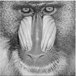
Figure 1. Test images: Lena (left), Baboon (center) and Man (right).

As a way to provide a reference, we also report the results obtained with ADMM, which is actually equivalent to the Split Bregman (SB) method [13, 9] for TV regularized problems. For a fair comparison, we implemented the generalized ADMM [6] with over and under relaxation factors, see also [5]. In the numerical tests we used $\rho_{k}=1$ or $\rho_{k}=1.5$ for all integer $k\geq 1$, in both methods. In Figure 2 we present some denoising results. It shows the noise contaminated images and the reconstructed images with the PMM. As in [13] iterations were terminated when condition $\left\|u_{k}-u_{k-1}\right\|/\left\|u_{k}\right\|\leq 10^{-3}$ was met; since this stopping criterion is satisfied faster than the stopping condition given by the KKT residuals, while yielding good denoised images.

Additionally, in Figure 3 we report the primal and dual residuals for the KKT optimality conditions for problem (62) for both methods, in some specific tests. The primal and dual residuals for the PMM were defined in section 4. For the ADMM the primal residual is also defined as $\nabla u_{k}-v_{k}$, i.e. it is the residual for the equality constraint at iteration $k$. The dual residual for the ADMM is defined as the residual for the dual feasibility condition (see equation (7) and the comments below). Since the exact solution of the problems are known we also plotted in Figure 3 the error $\left\|u_{k}-u^{\ast}\right\|$ vs iteration, where $u^{\ast}$ is the exact solution. In these experiments both methods were stopped at iteration $50$. It can be observed in Figure 3 that the speed of the PMM and ADMM measured by the residuals curves are very similar; however the residuals for the PMM decay faster, and this difference is more evident in the dual residual curve.

In Table 1 we present a more detailed comparison between the methods. It reports the iteration counts and total time, in seconds, required for the PMM and ADMM in the experiments. We observe that in the tests the PMM executed fewer iterations than ADMM, and the PMM was generally faster. We also observe that both methods accelerate when $\rho=1.5$.

(a) $\sigma=0.02$

(b) 12/14, $\rho=1.5$

(c) 20/21, $\rho=1$

(d) $\sigma=0.02$

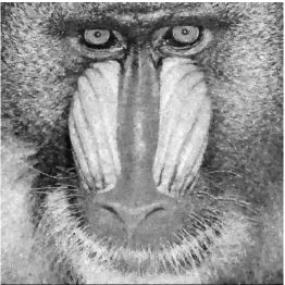
(e) 13/18, $\rho=1$

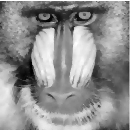
(f) 20/21, $\rho=1$

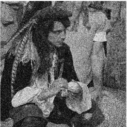
(g) $\sigma=0.06$

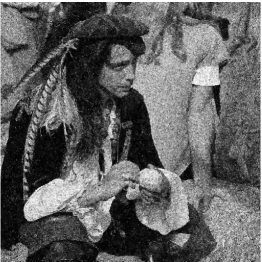
(h) 13/16, $\rho=1.5$

(i) 19/21, $\rho=1.5$

Figure 2. Denoising results. Images (a), (d) and (g) are contaminated with Gaussian noise, the value of variance ($\sigma$) is reported below each image. Images were denoised with $\zeta=20$ (center) and $\zeta=50$ (right). The value of $\rho$ and the number of iterations required to satisfy the stopping criterion, for both the PMM/ADMM, are listed below each image.

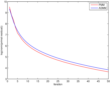
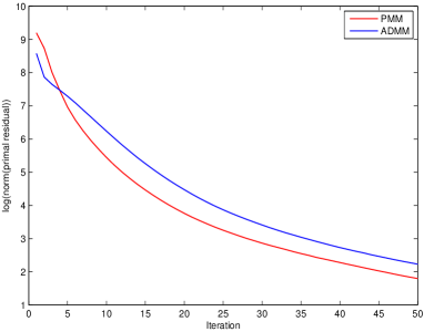
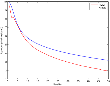
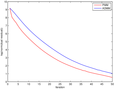
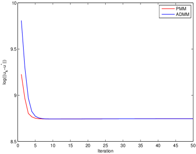
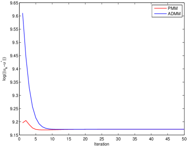
Figure 3. Residual curves of the PMM and ADMM for the TV denoising problems. (top) Primal error $\left\|\nabla u_{k}-v_{k}\right\|$ vs iteration number $k$. (center) Dual error $\left\|x_{k}-y_{k}\right\|$ vs iteration number $k$. (bottom) Error $\left\|u_{k}-u^{\ast}\right\|$ vs iteration number $k$ ($u^{\ast}$ is the exact solution). (left) Convergence results are for the tested image Lena with $\sigma=0.06$, $\zeta=50$ and $\rho=1.5$. (right) Convergence results are for the tested image Baboon with $\sigma=0.02$, $\zeta=20$ and $\rho=1$.

Image	$\zeta$	$\rho$	$\sigma$	PMM	ADMM
Lena	$20$	$1$	$0.02$	$13(2.789)$	$17(3.510)$
Lena	$20$	$1.5$	$0.02$	$12(1.803)$	$14(2.050)$
Lena	$50$	$1$	$0.06$	$19(2.855)$	$21(3.050)$
Lena	$50$	$1.5$	$0.06$	$17(2.642)$	$18(2.656)$
Baboon	$50$	$1$	$0.02$	$20(2.862)$	$21(2.811)$
Baboon	$50$	$1.5$	$0.02$	$19(2.920)$	$19(2.789)$
Baboon	$20$	$1$	$0.06$	$15(2.311)$	$21(2.928)$
Baboon	$20$	$1.5$	$0.06$	$13(2.025)$	$15(2.336)$
Man	$50$	$1$	$0.02$	$24(7.537)$	$24(7.364)$
Man	$50$	$1.5$	$0.02$	$21(6.700)$	$22(6.597)$
Man	$20$	$1$	$0.06$	$16(5.322)$	$21(6.540)$
Man	$20$	$1.5$	$0.06$	$13(4.395)$	$16(5.143)$
Man	$50$	$1$	$0.06$	$21(6.625)$	$24(7.371)$

Table 1. Iterations and computation times (seconds) in parenthesis required for the TV problem.

The operation of highest computational cost within each iteration of the PMM, and ADMM, for the TV problem, consists in solving problem (66). In our tests we solved this step for both algorithms using the Conjugate Gradient (CG) method with tolerance $10^{-5}$. This strategy consistently yielded convergence in fewer iterations when using the PMM. Table 2 presents the total number of iteration executed by the CG method in each algorithm for some specific experiments. In the tests presented both methods were stopped at iteration 20.

Image	$\zeta$	$\rho$	$\sigma$	PMM	ADMM
Lena	$20$	$1$	$0.02$	$108$	$117$
Lena	$20$	$1.5$	$0.06$	$101$	$110$
Baboon	$20$	$1.5$	$0.02$	$102$	$110$
Baboon	$50$	$1$	$0.02$	$121$	$122$
Man	$20$	$1.5$	$0.06$	$104$	$112$
Man	$50$	$1$	$0.06$	$124$	$126$

Table 2. Total number of iteration of CG method. Tests were stopped at iteration 20.

However, the authors of [13] observed that the ADMM (SB method) attained optimal efficiency executing, at each iteration of the algorithm, just a single iteration of an iterative method to solve problem (66). This inexact minimization can be justified by the convergence theory for the generalized ADMM developed by Eckstein and Bertsekas in [6], see also [9].

In [8], Eckstein and Svaiter generalized the projective-splitting algorithm for the sum of $N\geq 2$ maximal monotone operators, and they introduced a relative error criterion for approximately evaluating the proximal mappings. This framework suggests that the PMM can also admit inexact minimization for the subproblems. Indeed, as Figure 4 below shows, the PMM also yields good denoised images performing a single iteration of the CG method at each step of the algorithm.

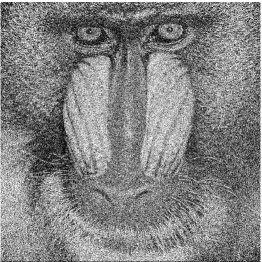
(a) $\sigma=0.06$

(b) 20(1.594), $\zeta=50$, $\rho=1$

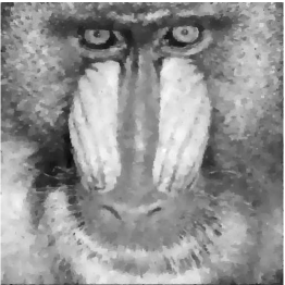
(c) 22(1.557), $\zeta=50$, $\rho=1$

(d) $\sigma=0.02$

(e) 14(2.436), $\zeta=20$, $\rho=1.5$

(f) 16(2.514), $\zeta=20$, $\rho=1.5$

Figure 4. Denoising with one iteration of CG method per iteration. (left) Noisy images, the value of variance is reported below each image. (center) Images denoised with PMM. (right) Images denoised with ADMM. The number of iterations, the total time in seconds (in parenthesis); as well as the used values of $\zeta$ and $\rho$ are displayed below each image.

5.2. Compressed sensing

In many areas of applied mathematics and computer science it is often desirable to reconstruct a signal from small amount of data. Compressed sensing is a signal processing technique that allow the reconstruction of signals and images from small number of measurements, provided that they have a sparse representation. This technique has gained considerable attention in the signal processing community since the works of Candès, Romberg and Tao [3], and of Donoho [4], and it has had a significant impact in several applications, for example in imaging, video and medical imaging.

For testing the PMM we consider a particular application of compressed sensing in Magnetic Resonance Imaging (MRI), which is an essential medical imaging tool. MRI is based on the reconstruction of an image from a subset of measurements in the Fourier domain. This imaging problem can be modeled by the optimization problem

(70) $$\min_{u}\,\,TV(u)+\dfrac{\zeta}{2}\left\|RFu-b\right\|_{F}^{2},$$

where $TV$ is the total variation norm (61), $F$ is the Discrete Fourier Transform, $R$ is a diagonal matrix, $b$ is the known Fourier data and $u$ is the unknown image that we wish to reconstruct.

The matrix $R$ has a $1$ along the diagonal at entries corresponding to the Fourier coefficients that were measured, and $0$ for the unknown coefficients. The second term in (70) induces the Fourier transform of the reconstructed image to be close to the measured data, while the TV term in the minimization enforces “smoothness” of the image. The parameter $\zeta>0$ provides a tradeoff between the fidelity term and the smoothness term.

Problem (70) can be posed as a linearly constrained minimization problem (1) in much the same manner as was done for the TV problem in the previous subsection. Therefore, to apply the PMM to (70) we take $f(u)=\dfrac{\zeta}{2}\left\|RFu-b\right\|^{2}_{F}$, $g(v)=\left\|v\right\|_{1}$, $M=\nabla$, $C=-I$ and $d=0$. The resulting minimization problems are

(71) $$v_{k}=\arg\min_{v}\,\,\left\|v\right\|_{1}-\left\langle z_{k-1}+\lambda w_{k-1},v\right\rangle+\dfrac{\lambda}{2}\left\|v\right\|^{2}_{F},$$

and

(72) $$u_{k}=\arg\min_{u}\,\,\dfrac{\zeta}{2}\left\|RFu-b\right\|^{2}_{F}+\left\langle z_{k-1}-\lambda v_{k},\nabla u\right\rangle+\dfrac{\lambda}{2}\left\|\nabla u\right\|^{2}_{F}.$$

Problem (71) can be solved explicitly using the shrink operator (3). Indeed, by the optimality conditions for this problem we have

$$v_{k}=\textbf{shrink}\left(\dfrac{1}{\lambda}z_{k-1}+w_{k-1},\dfrac{1}{\lambda}\right).$$

The optimality condition for the minimization problem (72) is

$$0=\zeta F^{T}R^{T}(RFu_{k}-b)+\nabla^{\ast}(z_{k-1}-\lambda v_{k})+\lambda\nabla^{\ast}\nabla u_{k},$$

or equivalently

$$(\zeta F^{T}R^{T}RF+\lambda\nabla^{\ast}\nabla)u_{k}=\zeta F^{T}R^{T}b-\nabla^{\ast}(z_{k-1}-\lambda v_{k}).$$

Thus, we obtain $u_{k}$, the solution of the system above, by

$$u_{k}=F^{T}(\zeta R^{T}R+\lambda F\nabla^{\ast}\nabla F^{T})^{-1}F(\zeta F^{T}R^{T}b-\nabla^{\ast}(z_{k-1}-\lambda v_{k})).$$

We tested the PMM on two synthetic phantom. The first is the digital Shepp-Logan phantom with dimensions $256\times 256$, which was created with the Matlab function “phantom”. For the compressed sensing problem of reconstructing this image we measured at random $25\%$ of the Fourier coefficients. The second experiment was done with a CS-Phantom of size $512\times 512$, which was taken from the mathworks web site. For this image we used $50\%$ of the Fourier coefficients. As stopping condition for these problems was used the criterion given by the residuals for the KKT conditions. More specifically, the PMM and ADMM were stopped when both, the primal and dual residual, associated with each method was less than a prefixed tolerance. Figure 5 shows the test images and their reconstructions using the PMM.

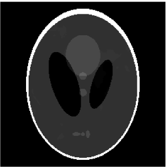
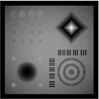
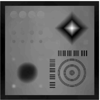
Figure 5. (left) Images used in compressed sensing tests. (right) The images reconstructed with the PMM. The Shepp-Logan phantom (top) was recovered with $25\%$ sampling and the CS-Phantom (bottom) with $50\%$.

For all the experiments we used $\zeta=500$, $\rho=1.5$ and $\lambda=1$, since we found that these choices were effective for both methods.

The performance of the PMM and ADMM can be seen in Figure 6, which reports the residuals curves for both methods, as were the error $\left\|u^{k}-u^{\ast}\right\|$, where $u^{\ast}$ is the exact solution. Observe that the primal curves for both methods are very similar along all iterations. However, the decay for the dual residual curve for the PMM is much faster than the dual residual for the ADMM.

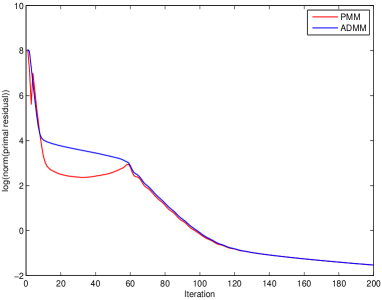
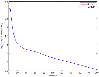
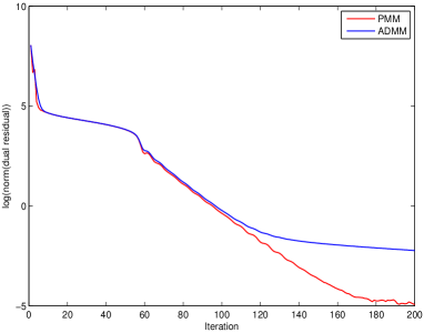
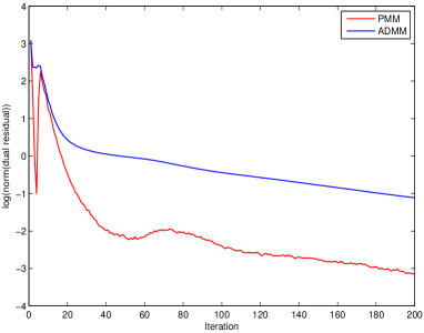
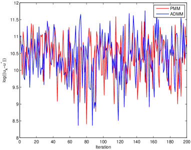
Figure 6. Residuals curves of the PMM and ADMM for the compressed sensing problems. (top) Primal error $\left\|\nabla u_{k}-v_{k}\right\|$ vs iteration number. (center) Dual error $\left\|x_{k}-y_{k}\right\|$ vs iteration number. (bottom) Error $\left\|u_{k}-u^{\ast}\right\|$ vs iteration number ($u^{\ast}$ is the exact solution). (left) Convergence results are for the Shepp-Logan phantom. (right) Convergence results are for the CS-Phantom.

5.3. The dual residual

It was observed in our numerical experiments that, despite the overall rate of decrease for the PMM and the ADMM are very similar, the dual variable in the PMM sequence is smaller than the ADMM dual variable. This could be an advantage for the PMM, and motivates us to study the performance of the method using a stopping criterion based on the dual residual.

In this subsection we present some preliminary computational results considering a termination condition that only uses information from the dual residual sequences. We use as test problems the TV (60) and CS (70) problems discussed in the previous subsections. The algorithms were run until condition

(73) $$\left\|d_{k}\right\|/(m*n)\leq 10^{-6}$$

was satisfied, where $d_{k}$ is the corresponding dual residual of the sequence at iteration $k$, and $m$ and $n$ are the dimensions of the images. In all the experiments we fixed $\lambda=1$.

Table 3 presents the number of iterations and time in seconds required for the PMM and ADMM to solve the problems in the experiments. We observe that the performances of the PMM and ADMM using criterion (73) are very similar in processing time and number of iterations when $\rho=1$. However, for $\rho>1$ the PMM is generally much faster than ADMM. We also notice that the PMM accelerates for $\rho>1$, when compared to the $\rho=1$ case, which does not always occur for the ADMM.

Figures 7 and 8 show the image reconstruction results for some tests. It can be observed in Figure 7 that for the TV problem both methods recover good images using (73). This is not surprising since the stopping criterion used in subsection 5.1 is more flexible than (73), and the restoration results were satisfactory (see subsection 5.1). It turns out that for the CS problem, although the termination condition considered in subsection 5.2 is more restrictive than (73), the PMM and ADMM can also reconstruct images with good quality using this last stopping criterion, as can be seen in Figure 8.

	PMM		ADMM
Problem	$\#$ It	time(s)	$\#$ It	time(s)
TV(Man, $\zeta=20$, $\rho=1$, $\sigma=0.03$)	98	154.708	114	161.859
TV(Man, $\zeta=20$, $\rho=1.8$, $\sigma=0.03$)	71	56.753	79	55.086
TV(Lena, $\zeta=40$, $\rho=1$, $\sigma=0.04$)	248	74.617	289	74.603
TV(Lena, $\zeta=40$, $\rho=1.5$, $\sigma=0.04$)	184	60.477	418	89.560
TV(Baboon, $\zeta=20$, $\rho=1$, $\sigma=0.01$)	137	45.185	148	45.251
TV(Baboon, $\zeta=20$, $\rho=1.3$, $\sigma=0.01$)	101	34.016	170	44.787
CS(Shepp-Logan, $\zeta=500$, $\rho=0.8$, $25\%$)	193	28.623	273	46.412
CS(Shepp-Logan, $\zeta=500$, $\rho=1$, $25\%$)	160	23.508	160	27.055
CS(Shepp-Logan, $\zeta=500$, $\rho=1.3$, $25\%$)	140	21.524	229	36.013
CS(Shepp-Logan, $\zeta=500$, $\rho=1.6$, $25\%$)	138	16.998	338	45.221

Table 3. Performance results using stooping criterion (73).

Figure 7. TV problem for the test image Lena, which was contaminated with Gaussian noise with variance $\sigma=0.04$. (left) Image denoised with PMM. (right) Image denoised with ADMM. The image was denoised using $\zeta=40$ and $\rho=1$.

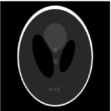
Figure 8. Compressed sensing problem for the test image Shepp-Logan phantom with $25\%$ sampling. (left) Image recovered with the PMM. (right) Image recovered with the ADMM. In the experiments were used $\zeta=500$ and $\rho=1.3$.

References

- [1] Brezis, H. Functional analysis, Sobolev spaces and partial differential equations. Universitext. Springer, New York, 2011.
- [2] Burachik, R. S., Sagastizábal, C. A., and Svaiter, B. F. -enlargements of maximal monotone operators: theory and applications. In Reformulation: nonsmooth, piecewise smooth, semismooth and smoothing methods (Lausanne, 1997), vol. 22 of Appl. Optim. Kluwer Acad. Publ., Dordrecht, 1999, pp. 25–43.
- [3] Candès, E. J., Romberg, J., and Tao, T. Robust uncertainty principles: exact signal reconstruction from highly incomplete frequency information. IEEE Trans. Inform. Theory 52, 2 (2006), 489–509.
- [4] Donoho, D. L. Compressed sensing. IEEE Trans. Inform. Theory 52, 4 (2006), 1289–1306.
- [5] Eckstein, J. Augmented lagrangian and alternating direction methods for convex optimization: A tutorial and some illustrative computational results. RUTCOR Research Reports 32 (2012).
- [6] Eckstein, J., and Bertsekas, D. P. On the Douglas-Rachford splitting method and the proximal point algorithm for maximal monotone operators. Math. Programming 55, 3, Ser. A (1992), 293–318.
- [7] Eckstein, J., and Svaiter, B. F. A family of projective splitting methods for the sum of two maximal monotone operators. Math. Program. 111, 1-2, Ser. B (2008), 173–199.
- [8] Eckstein, J., and Svaiter, B. F. General projective splitting methods for sums of maximal monotone operators. SIAM J. Control Optim. 48, 2 (2009), 787–811.
- [9] Esser, E. Applications of lagrangian-based alternating direction methods and connections to split bregman. CAM report 9 (2009), 31.
- [10] Gabay, D. Chapter ix applications of the method of multipliers to variational inequalities. Studies in mathematics and its applications 15 (1983), 299–331.
- [11] Gabay, D., and Mercier, B. A dual algorithm for the solution of nonlinear variational problems via finite element approximation. Computers & Mathematics with Applications 2, 1 (1976), 17–40.
- [12] Glowinski, R., and Marrocco, A. Sur l’approximation, par éléments finis d’ordre un, et la résolution, par pénalisation-dualité, d’une classe de problèmes de Dirichlet non linéaires. Rev. Française Automat. Informat. Recherche Opérationnelle Sér. Rouge Anal. Numér. 9, R-2 (1975), 41–76.
- [13] Goldstein, T., and Osher, S. The split Bregman method for -regularized problems. SIAM J. Imaging Sci. 2, 2 (2009), 323–343.
- [14] He, B., and Yuan, X. On the convergence rate of the Douglas-Rachford alternating direction method. SIAM J. Numer. Anal. 50, 2 (2012), 700–709.
- [15] Hiriart-Urruty, J.-B., and Lemaréchal, C. Convex analysis and minimization algorithms. II, vol. 306 of Grundlehren der Mathematischen Wissenschaften [Fundamental Principles of Mathematical Sciences]. Springer-Verlag, Berlin, 1993. Advanced theory and bundle methods.
- [16] Lions, P.-L., and Mercier, B. Splitting algorithms for the sum of two nonlinear operators. SIAM J. Numer. Anal. 16, 6 (1979), 964–979.
- [17] Minty, G. J. Monotone (nonlinear) operators in Hilbert space. Duke Math. J. 29 (1962), 341–346.
- [18] Monteiro, R. D. C., and Svaiter, B. F. Iteration-complexity of block-decomposition algorithms and the alternating direction method of multipliers. SIAM J. Optim. 23, 1 (2013), 475–507.
- [19] Moreau, J.-J. Proximité et dualité dans un espace hilbertien. Bull. Soc. Math. France 93 (1965), 273–299.
- [20] Passty, G. B. Ergodic convergence to a zero of the sum of monotone operators in Hilbert space. J. Math. Anal. Appl. 72, 2 (1979), 383–390.
- [21] Rockafellar, R. T. Convex analysis. Princeton Mathematical Series, No. 28. Princeton University Press, Princeton, N.J., 1970.
- [22] Rockafellar, R. T. On the maximal monotonicity of subdifferential mappings. Pacific J. Math. 33 (1970), 209–216.
- [23] Rudin, L. I., Osher, S., and Fatemi, E. Nonlinear total variation based noise removal algorithms. Phys. D 60, 1-4 (1992), 259–268. Experimental mathematics: computational issues in nonlinear science (Los Alamos, NM, 1991).
- [24] Tseng, P. Applications of a splitting algorithm to decomposition in convex programming and variational inequalities. SIAM J. Control Optim. 29, 1 (1991), 119–138.