Network reconstruction from infection cascades

Abstract

Accessing the network through which a propagation dynamics diffuse is essential for understanding and controlling it. In a few cases, such information is available through direct experiments or thanks to the very nature of propagation data. In a majority of cases however, available information about the network is indirect and comes from partial observations of the dynamics, rendering the network reconstruction a fundamental inverse problem. Here we show that it is possible to reconstruct the whole structure of an interaction network and to simultaneously infer the complete time course of activation spreading, relying just on single epoch (i.e. snapshot) or time-scattered observations of a small number of activity cascades. The method that we present is built on a Belief Propagation approximation, that has shown impressive accuracy in a wide variety of relevant cases, and is able to infer interactions in presence of incomplete time-series data by providing a detailed modeling of the posterior distribution of trajectories conditioned to the observations. Furthermore, we show by experiments that the information content of full cascades is relatively smaller than that of sparse observations or single snapshots.

Much effort has been devoted recently to the inverse problem of reconstructing the topology of a network from time series of a dynamical process acting on it. The methods proposed so far in the literature heavily rely on complete knowledge of the dynamical trajectories of some spreading process. In certain cases, when information about the time-series of the process is available, the problem can be, and has been, cast into relatively simple terms, since a sequence of time-consecutive states of a pair of nodes gives direct information about the potential interaction between them. In many cases, however, the set of available observations is much sparser, possibly on a much slower timescale than that of the dynamics, and often skipping the initial stages of the propagation which would give precious information about the initial condition. In particular, in an observation consisting on a single snapshot of the system there is no direct information about the interaction of nodes, as evidence of interaction indeed comes from variation of the state of nodes in time.

Let us take the example of second messenger cascades in a cell, and suppose the experimenter has access to the expression profile of a huge number of proteins in different cascades. Monitoring the exact time course of the concentration of each protein is currently challenging, if not unfeasible: one observes a concerted up and down-regulation of a big number of proteins, which naturally follow from a complex time course in a network of reciprocal protein-protein interactions. One is confronted with a similar information shortage in the context of epidemic spreading in a network of individuals: there is no information about who was the first one to contract the disease, and little is known about the underlying networks of contacts between individuals, which may even be dynamically changing over time.

Even though direct experimental data about contact networks in diverse contexts is being collected at a fast rate (Salathé et al., 2010; Isella et al., 2011; Rocha et al., 2010), there are some strong experimental and technical limitations to this collection, sometimes due to privacy protection regulations or concerns. However, knowledge of propagation networks would have a large list of benefits. First, it may allow to understand the propagation process better, including finding entry-points (e.g. the so called index case or patient zero in epidemiological jargon) of an ongoing epidemic. Second, it may allow to devise strategies to control the process in various ways, for example hindering the propagation (e.g. targeted vaccination) or favoring it (e.g. in the context of maximizing information diffusion on social networks, in viral or targeted advertising, etc). In this respect, a number of computational studies have introduced optimization methods based on message-passing that address the problem of containing (Altarelli et al., 2014a)or maximizing spreading (Altarelli et al., 2013a; Lokhov and Saad, 2016).

Recently, several approaches have been proposed for the problem of deducing the propagation network from time-series, based on a naive Bayes approach (Lokhov and Misiakiewicz, 2015) with efficient computations based on dynamic message-passing equations (Karrer and Newman, 2010; Lokhov et al., 2014), compressed sensing schemes (Shen et al., 2014), genetic (Wan et al., 2014) and dynamic programming algorithms (Wang et al., 2016), tensor decomposition (Yang et al., 2017) or on Monte Carlo sampling (Li and Li, 2017). These methods all share the need for observations at consecutive epochs.

Despite this recent progress, in most contexts the available observations of each cascade are sparse, noisy and discontinuous in time. In such situations, none of the methods proposed in the literature can be applied. One example is the problem of inferring functional contacts in signaling pathways, in which interacting proteins generate cascades of phosphorilation which eventually transmit signals from the cell membrane to the nucleus. Observations come in general from gene expression data, and the network to be inferred is a subnetwork of a large-scale protein-protein interaction network (PPI), also known as interactome. Although several experimental and computational approaches are able to identify candidate links of these networks, they lack in distinguishing false positive from true positive links (Bork et al., 2004; Valencia and Pazos, 2002; Yu and Fotouhi, 2006) that seems to be a challenging task. Social science and epidemiology offer another interesting domain of application, as one generally tries to infer the network of social contacts from a limited amount of sparse and noisy observations of some propagation histories.

Here we present a Bayesian technique that allows to uncover the complete functional structure (including its topology and parameters) of a network from a limited amount of single snapshots of the state of the network cascades. Starting from a functional parametrization of the posterior probability distribution of propagation trajectories, our technique builds on a Message Passing procedure that allows to compute, and then maximize, the likelihood of a given network structure. This computation can be performed efficiently thanks to Belief Propagation (BP), which is proven to be exact for tree graphs and has been successfully used in a variety of problems in general graphs with loops. Upon convergence, the parameters allow both to identify the network and the sources of the infection for each cascade with great accuracy. The method is effective on progressive propagation models like susceptible-infected (SI), susceptible-infected-removed (SIR), independent cascades (IC) and variants, including models with hidden variables (e.g. representing latency times). We called this method Gradient Ascent Belief Propagation (GABP)

Although the proposed inference machinery is very general, we focus on the well known Susceptible-Infected-Recovered (SIR)(Kermack and McKendrick, 1927) model, which describes those diseases in which infected individuals become immune to future infections after recovery (such as measles, rubella, chicken pox and generic influenza). More generally, SIR constitutes a good model for the spreading of rumor and information over a network or for the interaction dynamics among proteins.

Our minimal model of activity propagation in a network is very simple: if a node $i$ is active (Infected) at time $t$, it has a finite probability $\lambda_{ij}$ to activate (or infect) any of its neighbors $j$, which will in turn be active at time $t+1$. An active node will recover in each time-step with a (generally site-dependent) recovery probability $\mu_{i}$. Once recovered, individuals do not get sick anymore, and will not be able to infect other nodes. This will result in a propagation throughout the network, that we call a cascade.

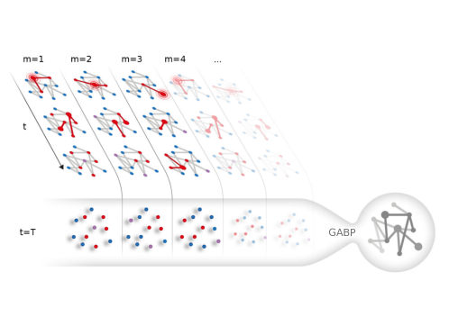
Let us then suppose that a number $M$ of independent realizations (or cascades) of the SIR dynamics can be observed. With independent cascades we mean that the realization of each stochastic process (in terms of infection and recovery times) do not affect the dynamics of other cascades. Identical realizations (same infected and recovered nodes, same infection and recovery times) are obviously strongly correlated but this does not limit the applicability of the method as far as each process is independent of one another. In the prototypical situation, the complete history of the propagation is not available: all we can observe is a number of “frozen” snapshots of a wave-front of the activity at a given time $T$, when all the states of the nodes in the network can be assessed to a reasonable extent of accuracy. Our aim is to identify the hidden network structure and the set of transmission probabilities for each link. Fig. 1 shows a cartoon representation of the problem.

Figure 1: Cartoon representation of the network reconstruction problem: $M$ independent cascades starting from different sources (highlighted in the first frame of each vertical stripe) are represented, with time flowing downward. Infected nodes are red, Susceptible nodes are blue and Recovered nodes are purple. The GABP algorithm is provided a set of $M$ snapshots taken $T$ time steps after the cascade onset: the goal is to reconstruct the functional interactions in the network $G$ as well as to identify the source of each cascade.

Results

A static formulation of the dynamical process

Reconstructing the unknown connectivity structure of the network is inevitably coupled to that of tracing back in time the entire history of the spreading process for each cascade $m$, $m\in\left\{1,...,M\right\}$, which in turn results in the identification of the sources of diffusion. Our approach builds on computing a joint posterior probability distribution over all cascades that are compatible with the observations, and then maximizing the likelihood of interaction parameters of the network at the same time. To set our notation, let us consider a weighted undirected graph $G=\left(V,E,\Lambda,\Omega\right)$ with a number $|G|$ of nodes, where $\Lambda=\left\{\lambda_{ij}\right\}_{ij\in E}$ play the role of edge-dependent infection probabilities in a SIR stochastic model, and that is also equipped with a set $\Omega=\left\{\mu_{i}\right\}_{i\in V}$ of site-dependent recovery probabilities. For directed graphs, we allow parameters $\lambda_{ij}\neq\lambda_{ji}$. Focusing, for the moment, on a single cascade, at any point in time each node $i$ will be in one of three possible states: susceptible $(S)$, infected $(I)$, and recovered/removed $(R)$. The state of node $i$ at time $t$ in each cascade $m$ is represented by a variable $x_{i}\left(t\right)\in\{S,I,R\}$, with $t$ in some discrete set. At each time step (e.g. a day) of the stochastic dynamics, an infected node $i$ can first spread the disease to each susceptible neighbor $j$ with given probability $\lambda_{ij}$, then recover with probability $\mu_{i}$. Each cascade is defined by the set of vectors $\mathbf{x}^{m}\left(t\right)$, with $m$ labeling the cascade, and we assume that for each cascade the initial state $\mathbf{x}^{m}\left(0\right)$ is composed of just one Infected node $i_{0}^{m}$, with all the other nodes in the network in the being in the Susceptible state. We will assume that we have access to the state of the nodes in the networks only $T^{m}=T$ steps after the initiation of each cascade.

Let us consider a node $i$ which gets infected at its infection time $t_{i}$: since it has a finite probability to pass the disease to a neighbor $j$ in each time step, this results in a stochastic transmission delay $s_{ij}$. In addition, the individual $i$ recovers at time $t_{i}+g_{i}$, with $g_{i}$ a stochastic recovery delay. Owing to the irreversibility of the spreading process, each cascade is fully specified by the quantities $\left\{t_{i},g_{i}\right\}_{i\in V}$ and $\left\{s_{ij}\right\}_{(i,j)\in E}$ for each node and each link in the network. It is then possible to construct a simple static graphical model representation of the dynamical process for each cascade on the grounds of the following simple observation: the time at which a given node $i$ gets infected only depends on the infection times of its neighbors $j$, and the infection delays of these nodes. Infection times $t_{i}>0$ are related by the deterministic equations

$$t_{i}=1+\min_{j\in\partial i}\left\{t_{j}+s_{ji}\right\}$$ (1)

which are a set of $|G|$ constraints encoding the infection dynamics, involving only local quantities at each node. Once the initial condition $\boldsymbol{x}\left(0\right)$ and stochastic quantities $s_{ij}$ and $g_{i}$ are thrown independently from their own distributions, the infection times are given deterministically by virtue of equation (1).

This observation was exploited in a series of works (Altarelli et al., 2013a, 2014b, 2014c) to develop a fully Bayesian method for approximating the whole probability distribution of the time evolution of the system, conditioned on some observations, and was originally used to identify the origin of the epidemic outbreak in SIR and similar models. The method is built on a Belief Propagation approximation (see Methods), which is exact on tree graphs and has proven successful in general networks with loops.

What if the underlying network is unknown, and so are the epidemic parameters $\left\{\lambda_{ij},\mu_{i}\right\}$? In a Maximum Likelihood approach, one needs to define the quantity $\mathcal{P}\left(\left\{\mathbf{x}^{m}\left(T\right)\right\}|\left\{\lambda_{ij}\right\},\left\{\mu_{i}\right\}\right),$ namely the likelihood of epidemic parameters with respect to observations, and then be able to maximize over the relevant parameters. Note that in a fully Bayesian framework, incorporating a priori information on the network topology or epidemic parameters is straightforward: it would lead to add a log-prior term $f_{\lambda,\mu}=\log\mathcal{P_{\lambda}}\left(\left\{\lambda_{ij}\right\}\right)+\log\mathcal{P_{\mu}}\left(\left\{\mu_{i}\right\}\right)$ to the log-likelihood to obtain a log-posterior. The log-likelihood of the parameters coincides with the so-called free-entropy of the system $\mathcal{L}\left(\left\{\lambda_{ij}\right\},\left\{\mu_{i}\right\}\right)=\log\mathcal{P}\left(\left\{\mathbf{x}^{m}\left(T\right)\right\}|\left\{\lambda_{ij}\right\},\left\{\mu_{i}\right\}\right)=-f\left(\left\{\lambda_{ij}\right\},\left\{\mu_{i}\right\}\right)$, which can be computed, consistently with the BP approximation, employing the Bethe decomposition (see Methods).

The BP method for the (cavity) marginal distributions of infection times can be then interleaved with simple log-likelihood climbing steps in a Gradient Ascent (GA) scheme, leading to a unique set of equations that are solved by iteration. In this setting, the computation of the gradient of the log-likelihood relies only on local updates involving the BP cavity messages. Ultimately all the information has to be processed locally at each node. That, in addition to other simplifications, entails a huge reduction of computational time, making the analysis of large-scale networks feasible efficiently (see Methods). One starts from a flat assignment of the parameters, and the initial fully connected network gets progressively pruned by means of the GA updates, eventually leading to a reconstructed network strongly resembling the real one.

Reconstructing random networks

We start by investigating three basic random network structures, namely Random Regular (RR), Erdos-Renyi (ER) and Barabasi-Albert (BA) scale-free networks: an impressive level of accuracy may be reached with a small number $M$ of observations. In a RR network, each node is connected at random with a fixed number of neighbors in the networks, whereas in the ER graph the number of neighbors is Poisson distributed. Scale-free networks, on the other hand, possess a power law degree distribution, and are known to capture some key ingredients of many real networks encountered in practical applications (for a review, see (Albert and Barabási, 2002)).

As a first step, a random graph is constructed, and a set of $M$ cascades are simulated, each one being an independent realization of the stochastic SIR process with a random initial source $i_{0}^{m}$. GABP is then run until the parameters $\lambda_{ij}$ and $\mu_{i}$ reach a stable value. Since the goal of the inference is two-fold, we use two different measures of the inference performance. For each cascade $m$, the nodes in the network are ranked in decreasing order with respect of the estimated probability of being the origin of the observed epidemic: the ability to identify the sources of the spreading is easily quantified by the rank of $i_{0}^{m}$, namely the position of $i_{0}^{m}$ in the ordered list.

On the other hand, a simple method for quantifying the accuracy of network reconstruction is the Receiver Operating Characteristic (ROC) curve, namely a plot of the true positive rate against the false positive rate in a binary classification problem. Constructing the ROC curve in the present case is very easy: the inferred values of $\lambda_{ij}$ are ranked in decreasing order, and one step upward in the ROC is taken if the link is present in the original graph (true positive) or one step rightward if the link is absent (false positive). The area under the ROC curve is a good indication of the discrimination ability: areas close to one signal a good discrimination between true links and non existent links. The reconstruction performances are compared to those of an empirical correlations based method. For each possible couple of nodes we compute, at the time of the observation $T$, the probability of having an edge $\left(i,\,j\right)$ as the mutual information (MI) between node $i$ and $j$; details of the calculations are reported in Mutual information. As for the case of parameters $\lambda_{ij}$, we construct ROC curves and we compute ROC areas from the set of correlation measures $m_{ij}$.

We report in Fig. 2 (a) a systematic investigation of the reconstruction performances of GABP and MI in the three types of random networks with an increasing number of cascades $M.$ The parameters of the infection are $\lambda=0.6$ and $\mu=0.4$ for all the experiments. For all values of $M$ GABP outperforms the MI method as the ROC areas associated with the GABP predictions are notably greater then the one obtained from MI. In the case of BA graphs, we notice smaller values of the ROC areas because, for these values of the parameters of the SIR dynamics, we observe huge epidemies in which at time $T$ almost all nodes are infected or recovered. This efficient spreading is caused by the presence of hubs that easily infect a good portion of the network in one time-step. In this regime and even for large value of $M$ there is not sufficient information to fully recover the true links of the graphs.

The ability to identify the sources of spreading (patient zero) is easily quantified by the rank $r_{0}^{(m)}$ of the true patient zero $i_{0}^{m}$ in each of the $M$ cascade: if $M$ is high enough so that enough information is conveyed on the underlying network structure, GABP is able to successfully identify most of the true initial spreaders in each cascade. This can be seen in Fig. 2 (b), that shows the distribution of $r_{0}^{(m)}$ for a value of $M=150$ in the three types of random networks considered here, which is fairly concentrated on low values of $r_{0}^{(m)}$.

Figure 2: a: Reconstruction accuracy in three types of random networks using GABP and MI. Each curve is an average over $30$ random instances of the area under the ROC curve, as a function of the number of observed cascades $M$ at time $T=5$. Epidemic parameters, $\lambda_{ij}=0.6$ and $\mu_{i}=0.4$, are the same for all the three type of networks. The size of the network is $|G|=50$. Blue curve (RR): Random Regular graphs with degree $d=4$; red curve (BA): Barabasi-Albert (scale-free) networks with average degree $d_{av}=4$; yellow curve (ER): Erdos-Renyi graphs with average degree $d_{av}=4$. Triangular and circular marks show GABP and MI results, respectively. b: Identification of initial spreaders. Each filled curve is the histogram of the rank of the true patient zero $i_{0}^{m}$ at $M=150$ for the three types of network. Histograms refer to $30$ random instances, thus considering a total of $30*150=4500$ independent cascades. c: Reconstruction accuracy versus connectivity. The blue curve is the area under the ROC curve in different instances of Random Regular graphs of size $|G|=50$ with increasing degree $d$. In each case, $M=50$ cascades are observed at time $T=7$. Recovery rate is fixed to$\mu_{i}=0.4$, $\lambda_{ij}$ is scaled down as degree increases in order to keep the size of epidemics roughly constant. Inset: area under the ROC curve as a function of the number of observed cascades $M$ in a random regular graph with degree $d=10$ (corresponding to the red point at the end of the blue curve in the main plot).

The reconstruction performance is expected to be substantially related to the density of the network. This can be investigated by systematically varying the degree of connectivity of a network, as it is shown in Fig. 2 (c), where the performance of GABP is assessed in a RR graph of size $|G|=50$ with an increasing connectivity degree $d$, from $d=4$ to $d=10$. The accurate reconstruction of denser networks requires, consequently, a larger number of cascades $M$.

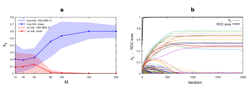
As can be seen in Fig. 3 (a), the distribution of inferred values of true links rapidly separates from the one of non-existent ones, that concentrates around vanishing values even for a very small number of observations. The strict separation of the two distributions confirms the results from the area under the ROC curve.

It is worth noting that GABP achieves a good level of reconstruction accuracy in a very small number of steps. The dynamics of the inferred $\lambda_{ij}$ as a function of iterations of the algorithm is exemplified in Fig. 3 (b). Even after a very small number of iterations, true links are clearly distinguished from non existent ones, as can be seen from the steep rise of the area under the ROC curve as a function of iterations: we observe that this kind of behavior is quite general and not restricted to the case $M=\mathcal{O}\left(N\right)$.

Figure 3: GABP rapidly identifies true links. a: average value of $\lambda_{ij}$ for true links (blue) versus non existent ones (red) as a function of the number of observed cascades in a Random Regular graph with size $|G|=50$, $\lambda_{ij}=0.6$, $\mu_{i}=0.4$ and $d=4$; shaded areas correspond to the intervals between the $10$th and the $90$th percentile in each distribution. b: the thin lines represent the$\lambda_{ij}$ values of a random subset of $200$ links in the case with $M=200$ cascades as a function of iterations of the GABP algorithm; black thick line: area under the ROC curve.

Reconstructing real networks

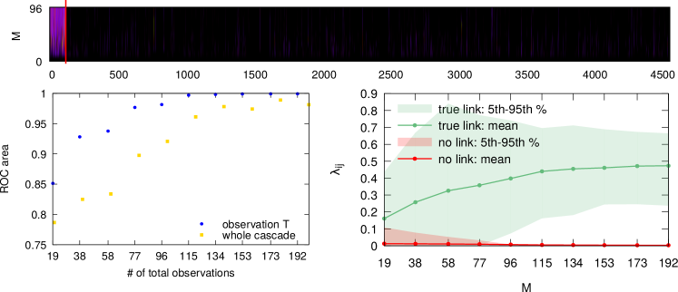
We tested the GABP algorithm on two different real interaction networks on which information about contacts is available for validation purposes. The first dataset consists of a networks of Twitter retweets (Rossi and Ahmed, 2013, 2015): the networks is composed of $|G|=96$ nodes, which represent Twitter users, linked through $|E|=117$ edges corresponding to retweets (these were collected from various social and political hash-tags). The average degree of a node in the network is $d_{av}=2$, with a minimum degree of $1$ and a maximum degree of $17$. Figure 4 shows the reconstruction performance in the retweet networks using two different observation paradigms: in the single-observation-per-cascade paradigm (which we considered as the standard case), the nodes state is available only once per cascade, whereas in the whole-cascade paradigm all nodes are observable at all times. It is apparent that an extremely accurate reconstruction is achievable with a number of cascade $M$ quite small compared to $|G|$.

Figure 4: Reconstruction performance of GABP in the network of retweets ($|G|=96$) with increasing number of independent cascades $M$. Epidemic parameters are $\lambda_{ij}=0.5$ and $\mu_{i}=0.4$, observation time $T=5$. Gold curve: area under ROC curve in the case where the state of the networks is fully observed at each time $t\in\left\{1,\dots,T\right\}$ for each cascade $m$. Blue curve: area under ROC curve in the case where the network is observed only at time $T$ in each cascade. Inset: average value of $\lambda_{ij}$ for true links (green) versus non existent ones (red) as a function of the number of observed cascades in the standard case (observation at time $T$ only); shaded areas correspond to the intervals between the $5$th and the $95$th percentile in each distribution.

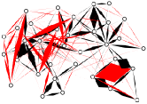
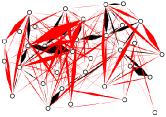
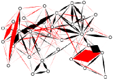
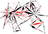
As another illustrative example, in Fig. 5 we show a pictorial representation of the reconstruction of the Zachary’s Karate Club network, a small social network which consists of $|G|=34$ nodes and $|E|=78$ edges, documenting the pairwise interactions over the course of three years among members of an university-based karate club. In this case, we simulated up to $M=102$ cascades and investigated the performance of the inference method with homogeneous parameters $\lambda=0.3$ and $\mu=0.4$ at increasing $M$. In Fig. 5, links not present in the actual graph are colored in red, and appear clearly distinguished from the true ones (colored in black) even for very small values of $M$.

$M=14$	$M=41$	M=68	$M=102$

Figure 5: Pictorial representation of the GABP performance in Zachary’s Karate Club network with an increasing number of cascades $M$. An edge is thrown between node $i$ and node $j$ if $\lambda_{ij}$ in non zero, the width of the edge being proportional to the value $\lambda_{ij}$. True links are colored in black, red links are not present in the original network.

For a more thorough representation of the reconstruction process in the Karate Club network, we show in Fig. 6 (Left) a color intensity plot of the dynamics of inference as the number of cascades is increased: true links are immediately identified, as the ROC area indicates (Right, blue curve).

It is very interesting to note that, while observing cascades in their entirety clearly conveys a lot of information on the network structure, if the total number of observations of the full state of the network is constrained, distributing these observations far apart in time pays better. This is clearly shown in Fig. 6 (Right) by the difference in the area under the ROC curve between the whole cascade scenario and the single-observation-per-cascade paradigm.

Figure 6: Left: Reconstruction performance of GABP in the Zachary’s Karate Club network with different numbers $M$ of independent cascades. $M$ is on the $y$ axis. The links are on the $x$ axis, ordered in such a way that the first $78$ are the true links in the original graph. The color intensity is proportional to the value $\lambda_{ij}$ for each putative link $\left(i,j\right)$ at increasing values of $M$. Right: area under the ROC curve (x axis) for increasing total observations (see text) of the entire networks (y axis, scale as in the left part). The blue curve corresponds to a single final observations per cascade at time $T=5$, the gold curve shows the case in which cascades are fully observed.

Detecting false positive links in PPI networks

A challenging problem in reconstructing protein-protein interaction networks consists in discriminating between true positive (TP) and false positive (FP) links. We show in this section how GABP algorithm can be used as a post-processing method to tackle this issue.

In our experiments we consider as ground-truth networks the giant components of five interactomes of the PSICQUIC dataset (Orchard, 2012) available on the software Cytoscape 3.5.1 (Shannon et al., 2003) (properties are summarized in Table (1)), while contact cascades are synthetically simulated with infection parameters $\lambda=0.8$ and $\mu=0.3$. To the true networks we add $Z=\alpha\left|E\right|$ extra edges, for $\alpha=\left[0.2,0.5\right]$, that mimic the presence of false positive interactions. This step is performed in a “scale-free” fashion: we first pick a node $i$ with probability proportional to its degree and we then connect it to a randomly uniformly chosen node $j\notin\partial i$. We then simulate $M\in\left[3,\,150\right]$ cascades on the true network and, from the final observations (at time $T=5$), we try to infer the transmission parameters $\lambda_{ij}$ associated with both true and false positive edges of the extended graph that, differently to the cases examined before, is not a fully connected graph. We compare our reconstructions to the ones obtained by a MI based method. In Fig. 7 we plot a table containing the areas under the ROC curves as a function of the number of cascades of the five interaction networks. Each row of the main figure corresponds to an organism and the columns run over $\alpha$. For all organisms the areas under the ROC curves of GABP results are significantly larger then those of MI reconstructions and they reach values above $0.9$ even when few cascades are available, i.e. $M=10$. Quite surprisingly, performances seem to be independent on the number of extra-edges suggesting that our method is quite robust in detecting false positive links when the extended graph to be pruned has a reasonable, but large, number of edges.

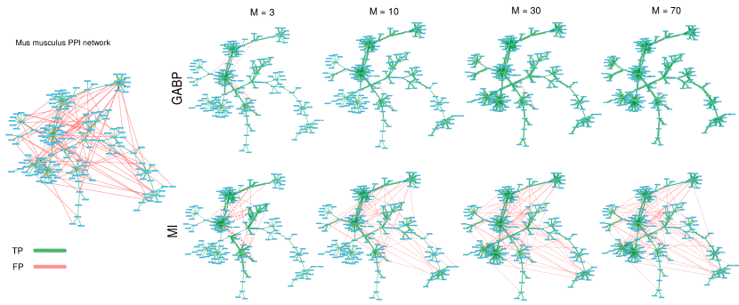
To underline the performances of GABP, we show in Fig. 8 (a) the Mus musculus interactome containing the true positive (green links) and 80 false positive edges (red links). The retrieved network for an increasing number of cascades is plotted in Fig. 8 (b); edges thickness is proportional to the inferred values of $\lambda_{ij}$ for GABP and to $m_{ij}$ for MI. It is worth noting that, for very few cascades ($M=3$), both GABP and MI are able to recognize almost all true links but GABP misclassifies fewer false positive than MI. When $M$ increases, GABP detects all true edges as the associated $\lambda_{ij}$ significantly increase and it incorrectly classifies only few false positive edges that, in any case, exhibit values of the infection parameters close to zero and negligible if compared to the ones associated with TP links. On the contrary MI distributes the weights over all the edges and, for large $M$, it is not able to sharply distinguish the two sets of links as some of the FP edges have comparable values of $m_{ij}$ to those of TP links.

Organism	|V|	|E|	Dataset name
Caenorhabditis Elegans	372	400	MINT (Orchard et al., 2014)
Drosophila Melanogaster	398	491	MINT
Homo Sapiens	801	1190	BHF-UCL
Mus Musculus	172	217	EBI-GOA-miRNA
Saccharomyces Cerevisiae	185	1476	UniProt (Consortium, 2017)

Table 1: Properties of the interactomes. This table shows the name of the organisms, the number of nodes and edges of the PPI networks and the name of the public datasets supported by PSICQUIC.

Figure 7: Plots of the ROC areas for GABP and MI interactomes predictions. Each row of the table corresponds to one of the five studied interactomes while each column to a different $\alpha$, the fraction of extra edges. Subplots show the areas under the ROC curves as a function of the number of cascades $M$ for GABP (blue line) and MI (red line).

Figure 8: False positive edges detection in PPI networks. (a) Mouse interactome of 172 nodes and 297 edges (217 true positive in green and 80 false positive in red). (b) the first (second) row shows the networks reconstructed by GABP (MI) for $M=\left\{3,\,10,\,30,\,70\right\}$. The thickness of each edge is proportional to the infection parameters of GABP and the mutual information among couples of nodes for MI; edges with weights smaller then $10^{-3}$ are not shown.

Inferring transmission probabilities

Let us now briefly consider a slightly different application of the general formalism presented so far. Suppose that the underlying network structure is known but little or any information is available on the transmission probabilities $\lambda_{ij}$, which are, in the general case, inhomogeneous. Our method can be easily accommodated so as to provide the maximum likelihood estimation of the quantities $\lambda_{ij}$. Starting from an initial assignment of the coupling parameters (we used $\lambda_{ij}\equiv 0.5)$ defined over a known topology, one seeks a fixed point of the coupled BP and gradient equations using GABP.

As an example, we consider a random regular graph of size $|G|=20$ with degree $d=4$, and evaluate the inference performance with increasing number of cascades $M$. Figure 9 (a) shows the value of the Mean Square Error $MSE=\frac{\sum_{\left(ij\right)\in E}\left(\lambda_{ij}-\lambda_{ij}^{true}\right)^{2}}{|E|}$ between the inferred transmission probabilities $\lambda_{ij}$ and the true ones, $\lambda_{ij}^{true}$. To better appreciate the quality of the inference, we show a scatter plot for two different values of $M$ in Figure 9 (b).

Figure 9: Reconstructing spreading couplings in inhomogeneous networks. a: mean squared reconstruction error $MSE=\frac{\sum_{i<j}\left(\lambda_{ij}-\lambda_{ij}^{true}\right)^{2}}{|E|}$ in a random regular graph of size $|G|=20$ and degree $d=4$, as a function of the number of observed cascades $M$. The network structure is known in advance. The spreading couplings $\lambda_{ij}^{true}$ have been extracted randomly from the homogeneous distribution in the interval $[0,1]$. The state of the network is observed only at time $T=5$ for each cascade. b: scatter plot of reconstructed transmission probabilities $\lambda_{ij}$ versus true spreading couplings $\lambda_{ij}^{true}$ for the cases $M=20$ and $M=400$, corresponding to the golden and green points in the left plot, respectively.

Discussion

We have presented a new method that allows to reconstruct a hidden network from limited information of activity propagations, and showed that the reconstruction performance is extremely accurate even when the number of snapshot observations is very small. This scheme can be effectively applied to the detection of false positive links in protein-protein interactions networks even when the number of candidate false edges is comparable to the effective number of true positive contacts. In this particular case it suffices very few independent cascades to correctly classify the great majority of the links.

There are several advantages of this approach over existing ones. The main one is that several inference problems can be treated under a unique formulation. Our technique can be easily extended to incorporate effects of unreliable observations, taking into account all those situations when some noise enters the measurements, or all those cases where Susceptible nodes cannot be distinguished from Recovered ones (Altarelli et al., 2014c). When a complete list of contact times between nodes is available, the construction of an equivalent network of timely dependent infection probability is straightforward, and the current approach has been proven to be effective.

Owing to the generality of the Bayesian method, the described technique is capable of dealing with a wide variety of irreversible spreading processes on networks. A possible simple generalization is to the (random) Bootstrap Percolation case where each node gets activated when aggregated input from neighbors overcome an intrinsic stochastic activation threshold of the node. These models are widely used to describe the features of dynamical processes in neuronal networks, and we consider this an exciting research direction.

Methods

Graphical model formulation of the spreading process

Let us first consider a single cascade on a network with a fixed topology. For a fixed initial configuration $\mathbf{x}\left(0\right)$, a realization of the stochastic process can be generated by drawing randomly a set of infection transmission delay $s_{ij}$ for all pairs $(ij)$ and the recovery times $g_{i}$ of each node $i$. The recovery times $\{g_{i}\}$ are independent random variables extracted from the geometric distributions $\mathcal{G}_{i}\left(g_{i}\right)=\mu_{i}\left(1-\mu_{i}\right)^{g_{i}}$, the delays $\{s_{ij}\}$ are conditionally independent random variables distributed according to a truncated geometric distribution,

$$\omega_{ij}\left(s_{ij}|g_{i}\right)=\begin{cases}\lambda_{ij}\left(1-\lambda_{ij}\right)^{s_{ij}},&s_{ij}\leq g_{i}\\ \left(1-\lambda_{ij}\right)^{g_{i}+1},&s_{ij}=\infty,\end{cases}$$ (2)

Note that we concentrate in the value $s_{ij}=\infty$ the mass of the distribution beyond the hard cut-off $g_{i}$ imposed by the recovery time. The joint probability distribution of infection and recovery times conditioned on the initial state is easily written:

$$\mathcal{P}\left(\mathbf{t},\mathbf{g}|\mathbf{x}\left(0\right)\right) =\sum_{\mathbf{s}}\mathcal{P}\left(\mathbf{s}|\mathbf{g}\right)\mathcal{P}\left(\mathbf{t}|\mathbf{x}\left(0\right),\mathbf{s},\mathbf{g}\right)\mathcal{P\left(\mathbf{g}\right)}$$

$$=\sum_{\mathbf{s}}\prod_{i,j}\omega_{ij}\left(s_{ij}|g_{i}\right)\prod_{i}\psi_{i}(t_{i},\{t_{k},s_{ki}\}_{k\in\partial i})\mathcal{G}_{i}(g_{i}),$$ (3)

where

$$\psi_{i}(t_{i},\{t_{k},s_{ki}\}_{k\in\partial i})=\delta(t_{i,}\mathbb{I}[x_{i}\left(0\right)\neq I](1+\min_{k\in\partial i}\{t_{k}+s_{ki}\}))$$ (4)

is a characteristic function which imposes on each node $i$ the dynamical constraint of equation (1).

Using the Bayes formula, the posterior probability of the initial configuration given an observation at time $T$ reads:

$$\mathcal{P}\left(\mathbf{x}\left(0\right)|\mathbf{x}\left(T\right)\right) \propto \sum_{\mathbf{t,g}}\mathcal{P}\left(\mathbf{x}\left(T\right)|\mathbf{t},\mathbf{g}\right)\mathcal{P}\left(\mathbf{t},\mathbf{g}|\mathbf{x}\left(0\right)\right)\mathcal{P}\left(\mathbf{x}\left(0\right)\right)$$ (5)

$$= \sum_{\mathbf{t},\mathbf{g},\mathbf{s}}\prod_{i,j}\omega_{ij}\prod_{i}\psi_{i}\mathcal{G}_{i}\gamma_{i}\zeta_{i}^{T}$$ (6)

where $\mathcal{P}\left(\mathbf{x}\left(0\right)\right)=\prod_{i}\gamma_{i}\left(x_{i}\left(0\right)\right)$ is a factorized prior on the initial infection with

$$\gamma_{i}(x_{i}\left(0\right))=\gamma\delta(x_{i}\left(0\right),I)+(1-\gamma)\delta(x_{i}\left(0\right),S)$$ (7)

for a generally small constant $\gamma$ (we don’t allow state $(R)$ at time 0). Note that the network state $\mathbf{x}\left(t\right)$ is a deterministic function of the set of infection and recovery times $(\mathbf{t},\mathbf{g})$, so that we obtain

$$\mathcal{P}\left(\mathbf{x}\left(T\right)|\mathbf{t},\mathbf{g}\right) = \prod_{i}\zeta_{i}^{T}\left(t_{i},g_{i},x_{i}\left(T\right)\right)$$ (8)

with $\zeta_{i}^{t}=\mathbb{I}\left[x_{i}\left(t\right)=S,t<t_{i}\right]+\mathbb{I}\left[x_{i}\left(t\right)=I,t_{i}\leq t<t_{i}+g_{i}\right]+\mathbb{I}\left[x_{i}\left(t\right)=R,t_{i}+g_{i}\leq t\right].$ Note that assuming $x_{i}\left(0\right)\in\left\{\left(S\right),\left(I\right)\right\}$, then $\psi_{i}(t_{i},\{t_{k},s_{ki}\}_{k\in\partial i})$ could be also rewritten equivalently as $\zeta_{i}^{0}\left(t_{i},g_{i},x_{i}\left(0\right)\right)[\delta(t_{i,}1+\min_{k\in\partial i}\{t_{k}+s_{ki}\})+\delta\left(t_{i},0\right)]$. Now, if we introduce a set of observational weights $\zeta_{i}^{m,T}$, one for each observation $m$, together with a set of priors priors $\zeta_{i}^{m,0}$, the posterior distribution of the initial states conditioned to observations, because of the assumption of independence, will be proportional to the product over all the single probability weights for each cascade $\mathcal{P}\left(\mathbf{x}^{1:M}\left(0\right)|\mathbf{x}^{1:M}\left(T\right)\right)\propto\prod_{m=1}^{M}\sum_{\mathbf{t}^{m},\mathbf{g}^{m}}\mathcal{P}\left(\mathbf{x}^{m}\left(T\right)|\mathbf{t}^{m},\mathbf{g}^{m}\right)\mathcal{P}\left(\mathbf{t}^{m},\mathbf{g}^{m}|\mathbf{x}^{m}\left(0\right)\right)\mathcal{P}\left(\mathbf{x}^{m}\left(0\right)\right)$ that taking into account equation (6) will take the form:

$$\mathcal{P}\left(\mathbf{x}^{1:M}\left(0\right)|\mathbf{x}^{1:M}\left(T\right)\right) \propto \prod_{m=1}^{M}\sum_{\mathbf{t}^{m},\mathbf{g}^{m},\mathbf{s}^{m}}\prod_{i<j}\omega_{ij}^{m}\prod_{i}\psi_{i}^{m}\mathcal{G}_{i}^{m}\gamma_{i}^{m}\zeta_{i}^{m,T}$$ (9)

where all the factors have been labeled with an extra cascade index $m$ and $\mathbf{x}^{1:M}\left(T\right)=\left(\mathbf{x}^{m}\left(T\right)\right)_{m=1,\dots,M}$. Since we have no a priori information on the graph topology, the product in the term $\prod_{i<j}\omega_{ij}^{m}$ runs over all the possible pair $i$ and $j$ in the set $V$, meaning that we always work in the setting of a fully connected network with weights $\left\{\lambda_{ij}\right\}$. If the number of cascades $M$ is large enough, the non zero elements of the matrix $\left\{\lambda_{ij}\right\}$ will signal, upon convergence of the GABP algorithm, the true links in the original graph, their value being informative of the heterogeneity of infection probabilities. The same holds for the set of recovery parameters $\left\{\mu_{i}\right\}$. Note that for $\lambda_{ij}=0$, (2) imposes the condition $s_{ij}=\infty$, meaning that $\left(ij\right)$ can be ignored in (1), effectively pruning the link from the equations.

Belief Propagation approach

Given a high dimensional probability distribution $M\left(\mathbf{z}\right)$ with a locally factorized interaction structure, computing marginals and aggregated quantities may be addressed with the use of a Message Passing procedure built on a cavity approximation for locally tree-like graphs (Yedidia et al., 2001, 2003; Mézard and Montanari, 2009). In the present problem, we obtain a full set of (cavity) marginal probabilities over the set of all the possible cascades compatible with the observations. BP is proven to be exact on tree graphs, and has been successfully employed on general loopy graphs under mild regularity conditions (Altarelli et al., 2013b, a)(Altarelli et al., 2013b, a).

To briefly describe the essence of the the method, let us consider a probability distribution over the variables $\mathbf{z}=\left\{z_{i}\right\}$ that has the following factorized form:

$$M\left(\mathbf{z}\right)=\frac{1}{Z}\prod_{a}\chi_{a}\left(\mathbf{z}_{a}\right)$$ (10)

where each $\chi_{a}$ is called compatibility function, or factor. We write $\mathbf{z}_{a}=\left\{z_{i}\right\}_{i\in\partial a}$ as the set of variables it depends on, $\partial a$ the subset of indices of variables in factor $\chi_{a}$, and accordingly $\partial i$ will be the subset of factors that depend on $z_{i}$. Belief Propagation equations are a set of self-consistent equations for the so-called cavity messages (or beliefs), a set of single-site probability distributions which are associated to each directed link in the graphical model representing to the joint distribution of equation (10). The general form of BP equations is the following:

$$p_{\chi_{a}\to i}\left(z_{i}\right) = \frac{1}{Z_{ai}}\sum_{\left\{z_{j}:j\in\partial a\setminus i\right\}}\chi_{a}\left(\mathbf{z}_{a}\right)\prod_{j\in\partial a\setminus i}m_{j\to\chi_{a}}\left(z_{j}\right)$$ (11)

$$m_{i\to\chi_{a}}\left(z_{i}\right) = \frac{1}{Z_{ia}}\prod_{b\in\partial i\setminus a}p_{\chi_{b}\to i}\left(z_{i}\right)$$ (12)

$$m_{i}\left(z_{i}\right) = \frac{1}{Z_{i}}\prod_{b\in\partial i}p_{\chi_{b}\to i}\left(z_{i}\right)$$ (13)

where the terms $Z_{ia},Z_{ai}$ and $Z_{i}$ are local partition function, serving as normalizers. To solve equations (11) and (12) an iterative procedure is typically used, where the cavity messages are initialized with uniform distributions and they are asynchronously updated until convergence to a fixed point (see e.g. (Yedidia et al., 2001; Mézard and Montanari, 2009) for an introduction). The BP equations can be thought as local update rules for messages in a so-called Factor Graph, a bipartite graph where each term $\chi_{a}$ is associated to a factor node, connected to all the variable nodes in the set $\mathbf{z}_{a}$ it depends on. A naive implementation of the BP scheme at the level of equation (9) would simply not work, since the corresponding graphical model has a loopy structure both at local and global scale. It is however possible to construct a disentangled factor graph by means of a re-parametrization of the cavity messages. We provide a brief description of this procedure in the Supplementary Methods. For a thorough discussion we refer the reader to previous works (see (Altarelli et al., 2014b), (Altarelli et al., 2014c)). Here we just want to stress that the modified factor graph is an enriched dual version of the original graph, whence the particular appeal of the method. In particular, this implies that Belief Propagation provides the exact Bayesian solution when the underlying network is acyclic.

While the computation of equation (12) is straightforward, the sum in equation (11) generally involves a number of steps growing exponentially with the size of $\partial a$. An efficient implementation of the BP equations for the posterior distribution is given in the Supplementary Methods. Once Belief Propagation converges, equation (13) can be used to compute the marginal probability $\mathcal{P}\left(t_{i}^{n}=0\mid\left\{\mathbf{x}^{m}\left(T\right)\right\}\right)$, which brings a posterior estimation of the probability for the node $i$ to be the active at time $t=0$ in the $m$th cascade.

Network reconstruction algorithm

We employ an alternating optimization scheme in which Belief Belief Propagation is coupled to a Maximum Likelihood strategy, implemented with a Gradient Ascent method. In the BP phase, the network parameters $\left\{\lambda_{ij},\mu_{i}\right\}$ are kept fixed and a solution is searched iteratively for equations (11) and (12). At this stage, the source can be located independently for each cascade looking at the single-site marginals $\mathcal{P}\left(x_{i}^{m}\left(0\right)|\left\{\mathbf{x}^{m}\left(T\right)\right\}\right)$. In the Maximum Likelihood phase, the log-likelihood of network parameters is maximized by means of a simple Gradient Ascent (GA) procedure. The gradient may be computed efficiently in the BP approximation. The likelihood $\mathcal{P}\left(\left\{\mathbf{x}^{m}\left(T\right)\right\}|\left\{\lambda_{ij}\right\},\left\{\mu_{i}\right\}\right)$ with respect to the network parameters is

$$Z\left(\left\{\lambda_{ij}\right\},\left\{\mu_{i}\right\}\right)=\prod_{m=1}^{M}\sum_{\mathbf{x}^{m}\left(0\right),\mathbf{t}^{m},\mathbf{g}^{m}}\mathcal{P}\left(\mathbf{x}^{m}\left(T\right)|\mathbf{t}^{m},\mathbf{g}^{m}\right)\mathcal{P}\left(\mathbf{t}^{m},\mathbf{g}^{m}|\mathbf{x}^{m}\left(0\right)\right)\mathcal{P}\left(\mathbf{x}^{m}\left(0\right)\right)$$

The logarithm of this quantity (log-likelihood) corresponds to the negative free energy of the model $\mathcal{L}\left(\left\{\lambda_{ij}\right\},\left\{\mu_{i}\right\}\right)=-f\left(\left\{\lambda_{ij}\right\},\left\{\mu_{i}\right\}\right)=\log Z\left(\left\{\lambda_{ij}\right\},\left\{\mu_{i}\right\}\right)$, and can be expressed as a sum of local terms depending only on the BP messages (see Supplementary Methods). BP updates for the distribution in equation (9) are then coupled to Gradient Ascent (GA) updates with respect to each network parameter, that take the form:

$$\lambda_{ij} \leftarrow \lambda_{ij}+\epsilon\frac{\partial\mathcal{L}}{\partial\lambda_{ij}}$$ (14)

$$\mu_{i} \leftarrow \mu_{i}+\epsilon\frac{\partial\mathcal{L}}{\partial\mu_{i}}$$ (15)

with $\epsilon$ a small multiplier parameter (we found $\epsilon=10^{-4}$ yields good results and stable convergence and used this value for all our simulations). The results presented in this work have been obtained by interleaving one BP step with a GA step: this simple scheme suffices to provide good joint estimates for the patient zero in each cascade, together with a remarkably good reconstruction of the underlying network. An alternative would consist in applying an expectation maximization (EM) scheme, in which alternatively BP equations are iterated to convergence (BP step) and parameters are fully optimized for fixed BP messages (EM step). However, the EM step requires the maximization of a high order polynomial that must be solved numerically in any case (e.g. in a GA scheme). We obtained faster convergence by alternating single GA and BP steps rather than alternating full convergence cycles of both steps.

Mutual information

For comparison we have tried to reconstruct the networks in interest using correlation based measures. At the observation time, we have computed the probabilities of observing edges $\left(i,j\right)$ as the mutual information between nodes $i$ and $j$:

$$m_{ij}=\sum_{\{x_{i},x_{j}\}}f_{ij}\left(x_{i}\left(T\right),x_{j}\left(T\right)\right)\log\frac{f_{ij}\left(x_{i}\left(T\right),x_{j}\left(T\right)\right)}{f_{i}\left(x_{i}\left(T\right)\right)f_{j}\left(x_{j}\left(T\right)\right)}$$ (16)

where $f_{ij},\,f_{i}\,$ are empirical probabilities computed as

$$f_{ij}\left(x_{i}\left(T\right),x_{j}\left(T\right)\right) =\frac{1}{M}\sum_{m}\delta_{x_{i}\left(T\right),\,x_{i}^{m}\left(T\right)}\delta_{x_{j}\left(T\right),\,x_{j}^{m}\left(T\right)}$$ (17)

$$f_{i}\left(x_{i}\left(T\right)\right) =\frac{1}{M}\sum_{m}\delta_{x_{i}\left(T\right),\,x_{i}^{m}\left(T\right)}$$ (18)

Appendix A BP equation: efficient disentangled implementation

We would like to use a factor graph representation that maintains the same topological properties of the original graph of contacts, in order to guarantee that BP is exact when the original contact graph is a tree. Following an approach developed in previous works (Altarelli et al., 2013b, a, 2014c), we proceed to disentangle the factor graph by grouping pairs of infection times $(t_{i},t_{j})$ in the same variable node. For convenience, we will keep all variable nodes $\{t_{i}\}$ but we will also introduce for each edge $(i,j)$ emerging from a node $i$ a set of copies $t_{i}^{(j)}$ of the infection time $t_{i}$, that will be forced to take the common value $t_{i}$ by including the constraint $\prod_{k\in\partial i}\delta(t_{i}^{(k)},t_{i})$ in an additional factor $\phi_{i}$.

The factors $\phi_{i}$ depend on infection times and transmission delays just through the sums $t_{i}^{(j)}+s_{ij}$, so that it is more convenient to introduce the variables $t_{ij}=t_{i}^{(j)}+s_{ij}$ and express the dependencies through the pairs $(t_{i}^{(j)},t_{ij})$.

Finally it is convenient to group the variable $g_{i}$ with the corresponding infection times $t_{i}$ in the same variable node, replace $g_{i}$ and $g_{j}$ by their copies $g_{i}^{(j)}$ and $g_{j}^{(i)}$ in the edge constraints $\omega_{ij}(t_{ij}-t_{i}^{(j)}|g_{i}^{(i)})$ and $\omega_{ji}(t_{ji}-t_{j}|g_{j}^{(i)})$ and impose the identity $\prod_{k\in\partial i}\delta(g_{i}^{(k)},g_{i})$ for each node $i$. The resulting disentangled factor graph appears in Fig. 10.

Figure 10: Disentangled Factor graph representation of the graphical model. White round nodes correspond to variables, gray rectangle nodes correspond to factors (or constraints). The topology of the disentangled factor graph follows the one of the original contact network.

An efficient form for the update equations of the $\psi_{i}$ factor nodes is the following:

$$p_{\psi_{i}\to j}\left(t_{i}^{\left(j\right)},t_{ji},g_{i}^{\left(j\right)}\right) \propto \sum_{g_{i},t_{i}}\sum_{\left\{t_{i}^{\left(k\right)},t_{ki},g_{i}^{\left(k\right)}\right\}}m_{i\to\psi_{i}}\left(t_{i},g_{i}\right)\times$$

$$\times\prod_{k\in\partial i\setminus j}m_{k\to\psi_{i}}\left(t_{i}^{\left(k\right)},t_{ki},g_{i}^{\left(k\right)}\right)\psi_{i}\left(t_{i},g_{i},\left\{\left(t_{i}^{(k)},t_{ki},g_{i}^{(k)}\right)\right\}_{k\in\partial i}\right)$$

$$\propto m_{i\to\psi_{i}}\left(t_{i}^{\left(j\right)},g_{i}^{\left(j\right)}\right)\sum_{t_{ki}}\prod_{k\in\partial i\setminus j}m_{k\to\psi_{i}}\left(t_{i}^{\left(j\right)},t_{ki},g_{i}^{\left(j\right)}\right)\times$$

$$\times\left[\delta\left(t_{i}^{(j)},0\right)+\delta\left(t_{i}^{(j)},\left(1+\min_{k\in\partial i}\left\{t_{ki}\right\}\right)\right)\right]$$

$$\propto \delta\left(t_{i}^{\left(j\right)},0\right)m_{i\to\psi_{i}}\left(0,g_{i}^{\left(j\right)}\right)\prod_{k\in\partial i\setminus j}\sum_{t_{ki}}m_{k\to\psi_{i}}\left(0,t_{ki},g_{i}^{\left(j\right)}\right)+$$

$$+\;m_{i\to\psi_{i}}\left(t_{i}^{\left(j\right)},g_{i}^{\left(j\right)}\right)\mathbb{I}\left(t_{i}^{\left(j\right)}\leq t_{ji}+1\right)\prod_{k\in\partial i\setminus j}\sum_{t_{ki}\geq t_{i}^{\left(j\right)}-1}m_{k\to\psi_{i}}\left(t_{i}^{\left(j\right)},t_{ki},g_{i}^{\left(j\right)}\right)$$

$$-\;m_{i\to\psi_{i}}\left(t_{i}^{\left(j\right)},g_{i}^{\left(j\right)}\right)\mathbb{I}\left(t_{i}^{\left(j\right)}<t_{ji}+1\right)\prod_{k\in\partial i\setminus j}\sum_{t_{ki}>t_{i}^{\left(j\right)}-1}m_{k\to\psi_{i}}\left(t_{i}^{\left(j\right)},t_{ki},g_{i}^{\left(j\right)}\right)$$

where in (A) we use the fact that

$$\delta\left(t_{i},\left(1+\min_{j\in\partial i}\left\{t_{ji}\right\}\right)\right)=\prod_{j\in\partial i}\mathbb{I}\left(t_{i}\leq t_{ji}+1\right)-\prod_{j\in\partial i}\mathbb{I}\left(t_{i}<t_{ji}+1\right).$$

Up to now, messages depend on the $T^{2}G$ values $\left(t_{i}^{\left(k\right)},t_{ki},g_{i}^{\left(k\right)}\right)$. It is however possible to use more concise representation, retaining just information on the relative timing between infection time $t_{i}^{\left(j\right)}$ for a node $i$ and the infection propagation time $t_{ji}$ on its link with node $j$, introducing the variables

$$\sigma_{ji}=1+\mbox{sign}\left(t_{ji}-\left(t_{i}^{\left(j\right)}-1\right)\right),$$ (22)

In order to switch to the simplified representation with $\left(\sigma_{ji},\sigma_{ij}\right)$ variables defined in (22) instead of $t_{ji},t_{ij}$ ones, we will proceed as follows. In equation (A) we can easily group the sums over different configurations of $\left(t_{ki},t_{i}^{(j)}\right)$ and write:

$$p_{\psi_{i}\to j}\left(t_{i}^{\left(j\right)},\sigma_{ji},g_{i}^{\left(j\right)}\right) \propto \delta\left(t_{i}^{\left(j\right)},0\right)m_{i\to\psi_{i}}\left(0,g_{i}^{\left(j\right)}\right)\prod_{k\in\partial i\setminus j}\sum_{\sigma_{ki}}m_{k\to\psi_{i}}\left(0,\sigma_{ki},g_{i}^{\left(j\right)}\right)+$$

$$+\;m_{i\to\psi_{i}}\left(t_{i}^{\left(j\right)},g_{i}^{\left(j\right)}\right)\mathbb{I}\left(\sigma_{ji}=1,2\right)\prod_{k\in\partial i\setminus j}\sum_{\sigma_{ki}=1,2}m_{k\to\psi_{i}}\left(t_{i}^{\left(j\right)},\sigma_{ki},g_{i}^{\left(j\right)}\right)$$

$$-\;m_{i\to\psi_{i}}\left(t_{i}^{\left(j\right)},g_{i}^{\left(j\right)}\right)\mathbb{I}\left(\sigma_{ji}=2\right)\prod_{k\in\partial i\setminus j}m_{k\to\psi_{i}}\left(t_{i}^{\left(j\right)},2,g_{i}^{\left(j\right)}\right)$$

Similarly, the outgoing message to the $(t_{i},g_{i})$ variable node is:

$$p_{\psi_{i}\to i}\left(t_{i},g_{i}\right) \propto \delta\left(t_{i},0\right)\prod_{k\in\partial i}\sum_{\sigma_{ki}}m_{k\to\psi_{i}}\left(0,\sigma_{ki},g_{i}\right)+$$

$$+\prod_{k\in\partial i}\sum_{\sigma_{ki}=1,2}m_{k\to\psi_{i}}\left(t_{i},\sigma_{ki},g_{i}\right)$$

$$-\prod_{k\in\partial i}m_{k\to\psi_{i}}\left(t_{i},2,g_{i}\right)$$

In the simplified  $\left(t,\sigma,g\right)$ representation for the messages, the update equation for the $\phi_{ij}$ nodes reads:

$$p_{\phi_{ij}\to j}\left(t_{j},\sigma_{ij},g_{j}\right)\propto\sum_{t_{i},\sigma_{ji},g_{i}}\Omega\left(t_{i},t_{j},\sigma_{ij},\sigma_{ji},g_{i},g_{j}\right)m_{i\to\phi_{ij}}\left(t_{i},\sigma_{ji},g_{i}\right)$$ (25)

where:

$$\Omega\left(t_{i},t_{j},\sigma_{ij},\sigma_{ji},g_{i},g_{j}\right)=\begin{cases}\chi\left(t_{i},t_{j},\sigma_{ij},g_{i}\right)&:t_{i}<t_{j},\leavevmode\nobreak\ \sigma_{ji}=2,\leavevmode\nobreak\ \sigma_{ij}\neq 2\\ \chi\left(t_{i},t_{j},\sigma_{ij},g_{i}\right)+\left(1-\lambda\right)^{g_{i}+1}&:t_{i}<t_{j},\leavevmode\nobreak\ \sigma_{ji}=2,\leavevmode\nobreak\ \sigma_{ji}=2\\ \chi\left(t_{j},t_{i},\sigma_{ji},g_{j}\right)&:t_{j}<t_{i},\leavevmode\nobreak\ \sigma_{ji}=2,\leavevmode\nobreak\ \sigma_{ji}\neq 2\\ \chi\left(t_{j},t_{i},\sigma_{ji},g_{j}\right)+\left(1-\lambda\right)^{g_{j}+1}&:t_{j}<t_{i},\leavevmode\nobreak\ \sigma_{ij}=2,\leavevmode\nobreak\ \sigma_{ji}=2\\ 1&:t_{i}=t_{j},\leavevmode\nobreak\ \sigma_{ji}=\sigma_{ij}=2\\ 0&:otherwise\end{cases}$$ (26)

and

$$\chi\left(t_{1},t_{2},\sigma,g\right)=\sum_{t=t_{1}}^{t_{1}+g}\delta\left(\sigma\left(t_{2},t\right),\sigma\right)\lambda\left(1-\lambda\right)^{t-t_{1}}$$ (27)

Simple algebra and precalculation of terms in (25)-(27) brings a significant optimization for updates involving the factor node $\phi_{ij}$ down to $O(TG^{2})$ operations per update.

 

Appendix B Gradient descent updates

The log-likelihood of the epidemic parameters is nothing but the free energy of the model. In the Bethe approximation, it can be expressed as a sum of local terms which only depends on the BP messages:

$$-f=\sum_{a}f_{a}+\sum_{i}f_{i}-\sum_{(ia)}f_{(ia)}$$ (28)

where

$$f_{a} = \log\left(\sum_{\left\{z_{i}:i\in\partial a\right\}}F_{a}\left(\left\{z_{i}\right\}_{i\in\partial a}\right)\prod_{i\in\partial a}m_{i\to a}(z_{i})\right)$$ (29)

$$f_{(ia)} = \log\left(\sum_{z_{i}}m_{i\to a}(z_{i})p_{F_{a}\to i}(z_{i})\right)$$ (30)

$$f_{i} = \log\left(\sum_{z_{i}}\prod_{b\in\partial i}p_{F_{b}\to i}(z_{i})\right)$$ (31)

Since $f$ is a function of all the BP messages, one would argue that this messages depend on the model parameters too, at every step in the BP algorithm. Actually, there is no need to consider this implicit $\left\{\lambda_{ij},\mu_{i}\right\}$ dependence if BP has reached its fixed point, that is when BP equations are satisfied and the messages are nothing else but Lagrange multipliers with respect to the constraint minimization of the Bethe free energy functional (Yedidia et al., 2001). In the present parametrization, the only explicit dependence of free energy on epidemic parameters is in the factor node terms $f_{a}$’s involving the compatibility functions $\phi_{ij}=\omega_{ij}\left(t_{ij}-t_{i}|g_{i}\right)\omega_{ji}\left(t_{ji}-t_{j}|g_{j}\right)$ and $\mathcal{G}_{i}\left(g_{i}\right)=\mu_{i}\left(1-\mu_{i}\right)^{g_{i}}$, and the gradient can be computed very easily. Please note that formulas below show the derivative of the free energy $f=-\mathcal{L}$: the GA updates of the log-likelihood only differ up to a minus sign. For the $\phi_{ij}$ nodes we have:

$$\frac{\partial f_{\phi_{ij}}}{\partial\lambda_{ij}}=\frac{\sum_{t_{i},t_{ji},g_{i},t_{j},t_{ij},g_{j}}\frac{\partial\phi_{ij}}{\partial\lambda_{ij}}\left(t_{i},t_{ji},g_{i},t_{j},t_{ij},g_{j}\right)m_{i\to\phi_{ij}}\left(t_{i},t_{ji},g_{i}\right)m_{j\to\phi_{ij}}\left(t_{j},t_{ij},g_{j}\right)}{\sum_{t_{i},t_{ji},g_{i},t_{j},t_{ij},g_{j}}\phi_{ij}\left(t_{i},t_{ji},g_{i},t_{j},t_{ij},g_{j}\right)m_{i\to\phi_{ij}}\left(t_{i},t_{ji},g_{i}\right)m_{j\to\phi_{ij}}\left(t_{j},t_{ij},g_{j}\right)}$$ (32)

where

$$\frac{\partial\phi_{ij}}{\partial\lambda_{ij}}=\begin{cases}1&t_{i}<t_{j}\mbox{ and }t_{i}=t_{ij}<t_{i}+g_{i}\\ -\left(g_{i}-t_{i}\right)\lambda_{ij}\left(1-\lambda_{ij}\right)^{g_{i}-t_{i}-1}&t_{i}<t_{j}\mbox{ and }t_{i}<t_{ij}=t_{i}+g_{i}\\ \left(1-\lambda_{ij}\right)^{t_{ij}-t_{i}}-\left(t_{ij}-t_{i}\right)\lambda_{ij}\left(1-\lambda_{ij}\right)^{t_{ij}-t_{i}-1}&t_{i}<t_{j}\mbox{ and }t_{i}<t_{ij}<t_{i}+g_{i}\\ 1&t_{j}<t_{i}\mbox{ and }t_{j}=t_{j}<t_{j}+g_{j}\\ -\left(g_{j}-t_{j}\right)\lambda_{ij}\left(1-\lambda_{ij}\right)^{g_{j}-t_{j}-1}&t_{j}<t_{i}\mbox{ and }t_{j}<t_{ji}=t_{j}+g_{j}\\ \left(1-\lambda_{ij}\right)^{t_{ji}-t_{j}}-\left(t_{ji}-t_{j}\right)\lambda_{ij}\left(1-\lambda_{ij}\right)^{t_{ji}-t_{j}-1}&t_{j}<t_{i}\mbox{ and }t_{j}<t_{ji}<t_{j}+g_{j}\\ 0&\mbox{else}\end{cases}$$ (33)

In the simplified $\left(t,\sigma,g\right)$ representation for the messages, equation (33) takes the form:

$$\frac{\partial\phi_{ij}}{\partial\lambda_{ij}}=\begin{cases}\chi\left(t_{i},t_{j},\sigma_{ij},g_{i}\right)&t_{i}<t_{j},\sigma_{ji}=2,\sigma_{ij}\neq 2\\ \chi\left(t_{i},t_{j},\sigma_{ij},g_{i}\right)-\left(g_{i}+1\right)\left(1-\lambda\right)^{g_{i}}&t_{i}<t_{j},\sigma_{ji}=2,\sigma_{ij}=2\\ \chi\left(t_{j},t_{i},\sigma_{ji},g_{j}\right)&t_{j}<t_{i},\sigma_{ji}=2,\sigma_{ij}\neq 2\\ \chi\left(t_{j},t_{i},\sigma_{ji},g_{j}\right)-\left(g_{j}+1\right)\left(1-\lambda\right)^{g_{j}}&t_{j}<t_{i},\sigma_{ji}=2,\sigma_{ij}=2\\ 0&otherwise\end{cases}$$ (34)

where:

$$\chi\left(t_{1},t_{2},\sigma,g\right)=\sum_{t=t_{1}}^{t_{1}+g}\delta\left(\sigma\left(t_{2},t\right),\sigma\right)\left(1-\lambda_{ij}\right)^{t-t_{1}}-\left(t-t_{1}\right)\lambda_{ij}\left(1-\lambda_{ij}\right)^{t-t_{1}-1}$$ (35)

For the $\mathcal{G}_{i}$ nodes we have:

$$\frac{\partial f_{\mathcal{G}_{i}}}{\partial\mu_{i}}=\frac{\sum_{g_{i}}\mathcal{\tilde{G}}_{i}(g_{i})m_{i\to\mathcal{G}_{i}}(g_{i})}{\sum_{g_{i}}\mathcal{G}_{i}(g_{i})m_{i\to\mathcal{G}_{i}}(g_{i})}$$ (36)

where

$$\mathcal{\tilde{G}}_{i}(g_{i})=\begin{cases}\left(1-\mu_{i}\right)^{g_{i}}-g_{i}\mu_{i}\left(1-\mu_{i}\right)^{g_{i}-1}&:g_{i}<G\\ G-G\left(1-\mu_{i}\right)^{G-1}&:g_{i}=G.\end{cases}$$ (37)

Author Contributions

AB, AI and APM contributed equally to this work.

References

- Salathé et al. [2010] Marcel Salathé, Maria Kazandjieva, Jung Woo Lee, Philip Levis, Marcus W. Feldman, and James H. Jones. A high-resolution human contact network for infectious disease transmission. Proceedings of the National Academy of Sciences, 107(51):22020–22025, 2010. doi: 10.1073/pnas.1009094108.
- Isella et al. [2011] Lorenzo Isella, Juliette Stehlé, Alain Barrat, Ciro Cattuto, Jean-François Pinton, and Wouter Van den Broeck. What’s in a crowd? analysis of face-to-face behavioral networks. Journal of Theoretical Biology, 271(1):166–180, February 2011. ISSN 0022-5193. doi: 10.1016/j.jtbi.2010.11.033.
- Rocha et al. [2010] Luis E. C. Rocha, Fredrik Liljeros, and Petter Holme. Information dynamics shape the sexual networks of internet-mediated prostitution. Proceedings of the National Academy of Sciences, 107(13):5706–5711, March 2010. ISSN 0027-8424, 1091-6490. doi: 10.1073/pnas.0914080107.
- Altarelli et al. [2014a] Fabrizio Altarelli, Alfredo Braunstein, Luca Dall’Asta, Joseph Rushton Wakeling, and Riccardo Zecchina. Containing epidemic outbreaks by message-passing techniques. Physical Review X, 4(2):021024, 2014a.
- Altarelli et al. [2013a] F. Altarelli, A. Braunstein, L. Dall’Asta, and R. Zecchina. Optimizing spread dynamics on graphs by message passing. Journal of Statistical Mechanics: Theory and Experiment, 2013(09):P09011, September 2013a. ISSN 1742-5468. doi: 10.1088/1742-5468/2013/09/P09011.
- Lokhov and Saad [2016] Andrey Y Lokhov and David Saad. Optimal deployment of resources for maximizing impact in spreading processes. arXiv preprint arXiv:1608.08278, 2016.
- Lokhov and Misiakiewicz [2015] Andrey Y Lokhov and Theodor Misiakiewicz. Efficient reconstruction of transmission probabilities in a spreading process from partial observations. arXiv preprint arXiv:1509.06893, 2015.
- Karrer and Newman [2010] Brian Karrer and M. E. J. Newman. Message passing approach for general epidemic models. Physical Review E, 82(1):016101, July 2010. doi: 10.1103/PhysRevE.82.016101.
- Lokhov et al. [2014] Andrey Y. Lokhov, Marc Mézard, Hiroki Ohta, and Lenka Zdeborová. Inferring the origin of an epidemic with a dynamic message-passing algorithm. Phys. Rev. E, 90:012801, Jul 2014. doi: 10.1103/PhysRevE.90.012801.
- Shen et al. [2014] Zhesi Shen, Wen-Xu Wang, Ying Fan, Zengru Di, and Ying-Cheng Lai. Reconstructing propagation networks with natural diversity and identifying hidden sources. Nature communications, 5, 2014.
- Wan et al. [2014] Xiang Wan, Jiming Liu, William K. Cheung, and Tiejun Tong. Inferring Epidemic Network Topology from Surveillance Data. PLOS ONE, 9(6):e100661, June 2014. ISSN 1932-6203. doi: 10.1371/journal.pone.0100661. URL http://journals.plos.org/plosone/article?id=10.1371/journal.pone.0100661.
- Wang et al. [2016] J. B. Wang, L. Wang, and X. Li. Identifying Spatial Invasion of Pandemics on Metapopulation Networks Via Anatomizing Arrival History. IEEE Transactions on Cybernetics, 46(12):2782–2795, December 2016. ISSN 2168-2267. doi: 10.1109/TCYB.2015.2489702.
- Yang et al. [2017] B. Yang, H. Pei, H. Chen, J. Liu, and S. Xia. Characterizing and Discovering Spatiotemporal Social Contact Patterns for Healthcare. IEEE Transactions on Pattern Analysis and Machine Intelligence, 39(8):1532–1546, August 2017. ISSN 0162-8828. doi: 10.1109/TPAMI.2016.2605095.
- Li and Li [2017] Xun Li and Xiang Li. Reconstruction of stochastic temporal networks through diffusive arrival times. Nature Communications, 8:15729, June 2017. ISSN 2041-1723. doi: 10.1038/ncomms15729. URL https://www.nature.com/articles/ncomms15729.
- Bork et al. [2004] Peer Bork, Lars J Jensen, Christian von Mering, Arun K Ramani, Insuk Lee, and Edward M Marcotte. Protein interaction networks from yeast to human. Current Opinion in Structural Biology, 14(3):292 – 299, 2004. ISSN 0959-440X. doi: https://doi.org/10.1016/j.sbi.2004.05.003. URL http://www.sciencedirect.com/science/article/pii/S0959440X04000776.
- Valencia and Pazos [2002] Alfonso Valencia and Florencio Pazos. Computational methods for the prediction of protein interactions. Current Opinion in Structural Biology, 12(3):368 – 373, 2002. ISSN 0959-440X. doi: https://doi.org/10.1016/S0959-440X(02)00333-0. URL http://www.sciencedirect.com/science/article/pii/S0959440X02003330.
- Yu and Fotouhi [2006] Jingkai Yu and Farshad Fotouhi. Computational approaches for predicting protein–protein interactions: A survey. Journal of Medical Systems, 30(1):39–44, Feb 2006. ISSN 1573-689X. doi: 10.1007/s10916-006-7402-3. URL https://doi.org/10.1007/s10916-006-7402-3.
- Kermack and McKendrick [1927] W. O. Kermack and A. G. McKendrick. A contribution to the mathematical theory of epidemics. Proceedings of the Royal Society of London. Series A, 115(772):700–721, August 1927. ISSN 1364-5021, 1471-2946. doi: 10.1098/rspa.1927.0118.
- Altarelli et al. [2014b] Fabrizio Altarelli, Alfredo Braunstein, Luca Dall’Asta, Alejandro Lage-Castellanos, and Riccardo Zecchina. Bayesian inference of epidemics on networks via belief propagation. Physical Review Letters, 112(11):118701, March 2014b. doi: 10.1103/PhysRevLett.112.118701.
- Altarelli et al. [2014c] Fabrizio Altarelli, Alfredo Braunstein, Luca Dall’Asta, Alessandro Ingrosso, and Riccardo Zecchina. The patient-zero problem with noisy observations. Journal of Statistical Mechanics: Theory and Experiment, 2014(10):P10016, 2014c.
- Albert and Barabási [2002] Réka Albert and Albert-László Barabási. Statistical mechanics of complex networks. Rev. Mod. Phys., 74:47–97, Jan 2002. doi: 10.1103/RevModPhys.74.47.
- Rossi and Ahmed [2013] Ryan A. Rossi and Nesreen K. Ahmed. rt-retweet - retweet networks, 2013. URL http://networkrepository.com/rt_retweet.php.
- Rossi and Ahmed [2015] Ryan A. Rossi and Nesreen K. Ahmed. The network data repository with interactive graph analytics and visualization. In Proceedings of the Twenty-Ninth AAAI Conference on Artificial Intelligence, 2015. URL http://networkrepository.com.
- Orchard [2012] Sandra Orchard. Molecular interaction databases. Proteomics, 12(10):1656–1662, May 2012. ISSN 1615-9861. doi: 10.1002/pmic.201100484.
- Shannon et al. [2003] P. Shannon, A. Markiel, O. Ozier, N. S. Baliga, J. T. Wang, D. Ramage, N. Amin, B. Schwikowski, and T. Ideker. Osgi alliance cytoscape: a software environment for integrated models of biomolecular interaction networks. Genome Res, 13(11):2498–2504, 2003.
- Orchard et al. [2014] Sandra Orchard, Mais Ammari, Bruno Aranda, Lionel Breuza, Leonardo Briganti, Fiona Broackes-Carter, Nancy H. Campbell, Gayatri Chavali, Carol Chen, Noemi del Toro, Margaret Duesbury, Marine Dumousseau, Eugenia Galeota, Ursula Hinz, Marta Iannuccelli, Sruthi Jagannathan, Rafael Jimenez, Jyoti Khadake, Astrid Lagreid, Luana Licata, Ruth C. Lovering, Birgit Meldal, Anna N. Melidoni, Mila Milagros, Daniele Peluso, Livia Perfetto, Pablo Porras, Arathi Raghunath, Sylvie Ricard-Blum, Bernd Roechert, Andre Stutz, Michael Tognolli, Kim van Roey, Gianni Cesareni, and Henning Hermjakob. The MIntAct project–IntAct as a common curation platform for 11 molecular interaction databases. Nucleic Acids Research, 42(Database issue):D358–363, January 2014. ISSN 1362-4962. doi: 10.1093/nar/gkt1115.
- Consortium [2017] The UniProt Consortium. UniProt: the universal protein knowledgebase. Nucleic Acids Research, 45(D1):D158–D169, January 2017. ISSN 0305-1048. doi: 10.1093/nar/gkw1099. URL https://academic.oup.com/nar/article/45/D1/D158/2605721.
- Yedidia et al. [2001] Jonathan S Yedidia, William T Freeman, and Yair Weiss. Bethe free energy, kikuchi approximations, and belief propagation algorithms. Advances in neural information processing systems, 13, 2001.
- Yedidia et al. [2003] Jonathan S. Yedidia, William T. Freeman, and Yair Weiss. Exploring artificial intelligence in the new millennium. chapter Understanding Belief Propagation and Its Generalizations, pages 239–269. Morgan Kaufmann Publishers Inc., San Francisco, CA, USA, 2003. ISBN 1-55860-811-7.
- Mézard and Montanari [2009] Marc Mézard and Andrea Montanari. Information, Physics, and Computation. Oxford University Press, January 2009. ISBN 9780198570837.
- Altarelli et al. [2013b] Fabrizio Altarelli, Alfredo Braunstein, Luca Dall’Asta, and Riccardo Zecchina. Large deviations of cascade processes on graphs. Physical Review E, 87(6):062115, June 2013b. doi: 10.1103/PhysRevE.87.062115.