2017

Yuan et al.

No Time to Observe: Adaptive Influence Maximization with Partial Feedback

No Time to Observe: Adaptive Influence Maximization with Partial Feedback

Jing Yuan Shaojie Tang The University of Texas at Dallas

Although influence maximization problem has been extensively studied over the past ten years, majority of existing work adopt one of the following models: full-feedback model or zero-feedback model. In the zero-feedback model, we have to commit the seed users all at once in advance, this strategy is also known as non-adaptive policy. In the full-feedback model, we select one seed at a time and wait until the diffusion completes, before selecting the next seed. Full-feedback model has better performance but potentially huge delay, zero-feedback model has zero delay but poorer performance since it does not utilize the observation that may be made during the seeding process. To fill the gap between these two models, we propose Partial-feedback Model, which allows us to select a seed at any intermediate stage. We develop two novel greedy policies that, for the first time, achieve bounded approximation ratios under both uniform and non-uniform cost settings.

1 Introduction

Since the seminal work of (Domingos and Richardson 2001), the influence maximization problem has attracted tremendous attention in recent years. This problem is first formalized and studied by (Kempe et al. 2003) as a discrete optimization problem. They study this problem under several diffusion models including independent cascade model and linear threshold model. They demonstrate that the influence maximization problem under both models are NP-hard, however, the objective function is monotone and submodular. Leveraging these nice properties, they propose an elegant greedy algorithm with constant approximation ratio. Since then, considerable work (Chen et al. 2013, Leskovec et al. 2007, Cohen et al. 2014, Chen et al. 2010, 2009, Tang et al. 2011, Tang and Yuan 2016, Tong et al. 2016, Yuan and Tang 2017) has been devoted to this topic and its variants.

However, majority of existing work fall into one of the following categories: full-feedback model (Golovin and Krause 2011) or zero-feedback model (Kempe et al. 2003). In the zero-feedback model, we have to commit the seed users all at once in advance, this strategy is also known as non-adaptive policy. In the full-feedback model, we select one seed at a time and wait until the diffusion completes, before selecting the next seed, this policy is also known as adaptive policy. This type of policy has better performance in terms of expected cascade because of its adaptivity, e.g, it allows us to adaptively choose the next seed after observing the actual spread resulting from previously selected seeds. However, the viral marketing in reality is often time-critical, implying that it is impractical, sometimes impossible, to collect the full status of the actual spread before selecting the next seed.

To fill this gap, we propose a generalized feedback model, called partial-feedback model, that captures the tradeoff between performance and delay. We adopt independent cascade model (IC) (Kempe et al. 2003), which is one of the most commonly used models, to model the diffusion dynamics in a social network. Unfortunately, we show that the objective under partial-feedback model and IC is not adaptive submodular, implying that existing results on adaptive submodular maximization does not apply to our model directly. To overcome this challenge, we develop two novel greedy policies, that, for the first time, achieve bounded approximation ratios under partial-feedback model. One nice feature of our policies is that we can balance the delay/performance tradeoff by adjusting the value of a controlling parameter.

1.1 Related Work

In (Domingos and Richardson 2001), they show that data mining can be used to determine potential seed users in viral market. Since then, there is a rich body of works that has been devoted to viral marketing problem. Most of existing works on this topic can be classified into two categories.

The first category is non-adaptive influence maximization: we must find a set of influential customers all at once in advance subject to a budget constraint. Kempe et al. (Kempe et al. 2003) first formalized and studied this problem under two diffusion models, namely Independent Cascade model and Linear Threshold model. (Chen et al. 2013, Leskovec et al. 2007, Cohen et al. 2014, Chen et al. 2010, 2009) study influence maximization problem under various extended models.

The second category is adaptive influence maximization, which is closely related to adaptive/stochastic submodular maximization Golovin and Krause (2011), Badanidiyuru et al. (2016), Tong et al. (2016), Yuan and Tang (2017). Existing studies mainly adopt full-feedback model, assuming that we can observe the full status of the previous cascade before selecting the next seed. We relax this assumption by incorporating partial-feedback and develop two adaptive policies that achieve the first bounded approximation ratios under partial-feedback model.

2 Network Model and Diffusion Process

2.1 Independent Cascade Model

A social network is modeled as a directed graph $G=(V,E)$, where $V$ is a set of $n$ nodes and $E$ is a set of social ties. We adopt independent cascade model (Kempe et al. 2003) to model the diffusion dynamics in a social network. Each node $v\in V$ is associated with a cost $c_{v}$, each edge $(u,v)$ in the graph is associated with a propagation probability $p_{uv}$, which is the probability that node $u$ independently influences node $v$ in the next slot after $u$ is influenced. The expected cascade of $U$, which is the expected number of influenced nodes given seed set $U$, is denoted as $I(U)$.

2.2 The Feedback Model

Majority of existing work adopt one of the following feedback models: zero-feedback model or full-feedback model.

Zero-feedback Model: During the seeding process, we can not observe anything about the resulting spread of adoption. Since there is no benefit in “waiting”, we can simply commit the seeds all at once in advance. This model is equivalent to traditional non-adaptive influence maximization problem which has been well studied in the literature, (Kempe et al. 2003) showed that the utility function under this model is submodular and then propose a Greedy algorithm whose performance is lower bounded $(1-1/e)$ times the optimal non-adaptive solution. It is still unclear about the upper bound on the adaptivity gap, e.g., the performance gap between non-adaptive and adaptive solutions.

Full-feedback Model: We select one seed at a time and wait until the diffusion completes, before selecting the next seed, this policy is also known as adaptive policy. In particular, after selecting a seed $u$, we can observe the status of all edges existing $v$, where $v$ is any node that is reachable from $u$ via live edges in the full realization. For this model, (Golovin and Krause 2011) introduced the concept of adaptive submodularity and proposed a Greedy algorithm has a $(1-1/e)$ approximation guarantee.

As discussed in Section 1, full-feedback (resp. zero-feedback) model has better (resp. poorer) performance but potentially huge (resp. small) delay. To fill the gap between these two models, we propose partial-feedback model, which generalizes the previous two models by allowing us to select the next seed at some intermediate stage.

Based on independent cascade model, we next introduce the concept of diffusion realization (Golovin and Krause 2011) and other related concepts.

Definition 2.1 (Diffusion Realization)

Let $\psi((u,v))\in\{0,1,?\}$ denote the state of $(u,v)$ given realization $\psi$ where $\psi((u,v))=0$ means that $(u,v)$ is blocked, $\psi((u,v))=1$ means that $(u,v)$ is live, and $\psi((u,v))=?$ means that the state of $(u,v)$ is unknown. We represent the state of the diffusion stage using function $\psi:E\rightarrow\{0,1,?\}$, called diffusion realization.

Definition 2.2 (Partial and Full Realization)

Let $\mathrm{dom}(\psi)=\{(u,v):\psi((u,v))\in\{0,1\}\}$ denote the set of edges observed in $\psi$. $\psi$ is a full realization if $\mathrm{dom}(\psi)=E$ (i.e., all edges are observed in full realization). Otherwise, $\psi$ is called partial realization.

Definition 2.3 (Intermediate and Final Realization)

Given a realization $\psi$ of seeds $S$, we say $\psi$ is a final realization if $\mathrm{dom}(\psi)$ is finalized (i.e., we can not observe more edges other than $\mathrm{dom}(\psi)$ by waiting longer). Otherwise, $\psi$ is called intermediate realization. Let $X(S)$ denote the set of all final realizations of $S$.

Definition 2.4 (Subrealization and Superrealization)

A realization $\psi_{a}$ is consistent with a realization $\psi_{b}$ (i.e., $\psi_{a}\thicksim\psi_{b}$) if they are equal everywhere in $\mathrm{dom}(\psi_{a})\cap\mathrm{dom}(\psi_{b})$. We say $\psi_{a}$ is a subrealization of $\psi_{b}$ (or equivalently $\psi_{b}$ is a suprealization of $\psi_{a}$) if $\psi_{a}$ is consistent with $\psi_{b}$ and $\mathrm{dom}(\psi_{a})\subseteq\mathrm{dom}(\psi_{b})$, or $\psi_{a}\subseteq\psi_{b}$. We say $\psi_{b}$ is a final superrealization of $\psi_{a}$ given $S$ if $\psi_{b}\in X(S)$ and $\psi_{b}\supseteq\psi_{a}$ (i.e., $\psi_{b}$ is a final realization and $\psi_{b}$ is a superrealization of $\psi_{a}$).

Consider an intermediate realization $\psi$ of seeds $S$, let $X_{\mathrm{final}}(S|\psi):=\{\phi:\phi\in X(S),\phi\supseteq\psi\}$ denote the set of all final realizations of $S$ given $\psi$.

3 Problem Formulation

Under the partial-feedback model, we perform the decision process in a sequential manner where the decision made in each round is depending on the current observation of the network status and the remaining budget.

Definition 3.1 (Adaptive Policy)

We define our adaptive policy $\pi:(\psi,S)\rightarrow v$, which is a function from the current “observation” $\psi$ and the set of existing seeds $S$ to $v$, specifying which seed to pick next given a particular set of observations.

Definition 3.2 (Policy Concatenation)

Given two policies $\pi_{a}$ and $\pi_{b}$, we use $\pi_{a}@\pi_{B}$ to denote a policy that runs $\pi_{a}$ first, and then runs policy $\pi_{b}$, ignoring the information obtained from running $\pi_{a}$.

We use $\Psi$ to denote a random realization. Assume there is a known prior probability distribution $\Pr[\psi]:=\Pr[\Psi=\psi]$ over $W$ which is the universe of all possible full realizations. Given a full realization $\psi$, let $S_{\psi}$ denote all seeds picked by $\pi$ under $\psi$, and $c(S_{\psi})=\sum_{v\in S_{\psi}}c_{v}$ denote the total cost of $S_{\psi}$. The expected cascade of a policy $\pi$ is

$$f(\pi)=\mathbb{E}[I(S_{\Psi}|\Psi)]=\sum_{\psi\in W}\Pr[\psi]I(S_{\psi})$$

where $I(S_{\psi})$ denotes the cascade of $S_{\psi}$ given realization $\psi$, e.g., all nodes that are reachable from $S_{\psi}$ under $\psi$. The goal of the adaptive influence maximization problem is to find a policy $\pi$ such that

  Maximize $f(\pi)$ subject to: $$c(S_{\psi})\leq B,\forall\psi\in W$$

We first show that the objective is not adaptive submodular under partial feedback model. The concept of adaptive submodularity is a generalization of submodularity to adaptive policies: we say a function $f$ is adaptive submodular if adding an element $e$ to a realization $\psi$ increases $f$ at least as much as adding $e$ to a superset of $\psi$. Since the Myopic Feedback model proposed in (Golovin and Krause 2011) is a special case of our partial-feedback model, we borrow the same counter example from their work to prove the following lemma.

Theorem 3.3

(Golovin and Krause 2011) The objective $f$ under partial-feedback model is not adaptive submodular.

First of all, we want to emphasize the difference between “round” and “slot”. One round corresponds to one execution of our algorithm, while one slot corresponds to one step of information propagation. In the rest of this paper, we use $|\cdot|$ to denote the size of a set.

4 $\alpha$-Greedy Adaptive Policy with Partial Feedback

In this section, we present the first adaptive policy, called $\alpha$-Greedy policy, and analyze its performance bound. For ease of presentation, we start with uniform cost setting where all nodes have identical costs. Then we extend this result to non-uniform cost setting.

4.1 Uniform Cost

We first study the case with uniform cost, e.g., $\forall v\in V:c_{v}=1$. Since each node has the same cost, the budget constraint can be reduced to cardinality constraint, e.g., the number of seeds that can be selected is upper bounded by $B$.

4.1.1 Policy Description

$\alpha$-Greedy policy $\pi^{\alpha}$ (Algorithm 1) is performed in a sequential greedy manner as follows: After observing the current partial realization, we choose to either wait for another slot or select the next seed immediately that maximizes the expected marginal benefit. This process iterates until the budget is used up.

1. Start with slot $t=1$, seeds $S=\emptyset$, and a control parameter $\alpha\in[0,1]$;

2. Suppose we have made observations $\psi_{[t]}$ at slot $t$, let $p_{v}(S;\psi_{[t]})$ denote the activation probability of $v$ given seeds $S$ and observation $\psi_{[t]}$, and let $f(S|\psi_{[t]})=\sum_{v\in V}p_{v}(S;\psi_{[t]})$ denote the expected cascade under the same setting. Define ${O(S;\psi_{[t]})}:=\{v:p_{v}(S;\psi_{[t]})=0\}$ as the set of nodes whose activation probability is zero under $\psi_{[t]}$ and $S$. We then examine the following condition.

   $$\frac{f(S|\psi_{[t]})}{|V\setminus O(S;\psi_{[t]})|}\geq\alpha$$ (1)

   If condition (1) is satisfied, select $\arg\max_{u\in V}\Delta_{u}(S;\psi_{[t]})$ where $\Delta_{u}(\psi_{[t]};S)=f(\{u\}\cup S|\psi_{[t]})-f(S|\psi_{[t]})$ denotes the expected marginal benefit of $v$ given existing seeds $S$ and partial realization $\psi_{[t]}$ (i.e., we select a node that maximizes the expected marginal benefit). Otherwise, if condition (1) is not satisfied, we wait for another slot.

3. This process iterates until the budget is used up.

Condition (1) can be interpreted as follows: we will not select the next seed until the average activation probability of all nodes with non-zero activation probability is sufficiently high. Note that this condition can always be satisfied when we reach a final realization (i.e., $\frac{f(S|\psi_{[t]})}{|V\setminus O(S;\psi_{[t]})|}=1$ when $\psi_{[t]}$ is a final realization). We use $\alpha$ to control the tradeoff of delay and performance. In particular, a larger $\alpha$ indicates longer delay but better performance. For example, if we set $\alpha=1$, our model becomes full-feedback model, that is, we must wait until every node is either in active state or non-active state, before selecting the next seed. On the other hand, if we set $\alpha=0$, our model is reduced to zero-feedback model, implying that we can select all seeds in advance.

It was worth noting that we may select multiple seeds in one slot as long as condition (1) holds, thus one slot may contain multiple rounds.

Algorithm 1 $\alpha$-Greedy Policy: $\pi^{\alpha}$

Input: $0\leq\alpha\leq 1$.
Output: $S$.

1:  $S=\emptyset$; $t=0$;

2:  $S\leftarrow S\cup\{\arg\max_{u\in V}\Delta_{u}(S|\psi_{[t]})\}$;

3:  $B\leftarrow B-1$; $t\leftarrow t+1$

4:  while $B\geq 0$ do

5:     if $\frac{f(S|\psi_{[t]})}{|V\setminus O(S;\psi_{[t]})|}\geq\alpha$ then

6:        $S\leftarrow S\cup\{\arg\max_{u\in V}\Delta_{u}(S|\psi_{[t]})\}$;

7:        $B\leftarrow B-1$;

8:     else

9:        $t\leftarrow t+1$; update $\psi_{[t]}$;

10:  return  $S$

4.1.2 Performance Analysis

Let $\pi_{[t]}$ denote the level-$t$-truncation of $\pi$ obtained by running until it terminates or until slot $t$. For every $1\leq i\leq B$, assume the $i$-th seed is added to $S$ at slot $t_{i}$ (i.e., $\frac{f(S|\psi_{[t_{i}]})}{|V\setminus O(S;\psi_{[t_{i}]})|}\geq\alpha$). For brevity, we use $O$ to denote $O(S;\psi_{[t_{i}]})$. Let $f^{O}(S|\psi_{[t_{i}]})=\sum_{v\in O}p_{v}(S;\psi_{[t_{i}]})$ denote the expected cascade in ${O}$ given seeds $S$ and observation $\psi_{[t_{i}]}$. We use $\pi^{*}$ to denote the optimal adaptive policy. In the rest of this paper, let $f(\pi|\psi)$, $f^{O}(\pi|\psi)$, $f^{V\setminus O}(\pi|\psi)$ denote respectively the expected cascade of $\pi$ in $V$, $O$, $V\setminus O$ under realization $\psi$. In order to prove the main theorem (Theorem 4.3), we first prove two preparatory lemmas (Lemma 4.1 and Lemma 4.2).

Lemma 4.1

For any $1\leq i\leq B$ and $0<\alpha\leq 1$, we have

$$f(\pi^{*}|\psi_{[t_{i}]})-f(\pi^{\alpha}_{[t_{i}]}|\psi_{[t_{i}]})/\alpha\leq f^{O}(\pi^{*}|\psi_{[t_{i}]})-f^{O}(\pi^{\alpha}_{[t_{i}]}|\psi_{[t_{i}]})$$

Proof: First, we have

$$f(\pi^{*}|\psi_{[r_{i}]})-f(\pi^{\alpha}_{[t_{i}]}|\psi_{[t_{i}]})/\alpha$$ (2)

$$=(f^{O}(\pi^{*}|\psi_{[t_{i}]})-f^{O}(\pi^{\alpha}_{[t_{i}]}|\psi_{[t_{i}]})/\alpha)+(f^{V\setminus O}(\pi^{*}|\psi_{[t_{i}]})-f^{V\setminus O}(\pi^{\alpha}_{[t_{i}]}|\psi_{[t_{i}]})/\alpha)$$ (3)

$$\leq(f^{O}(\pi^{*}|\psi_{[t_{i}]})-f^{O}(\pi^{\alpha}_{[t_{i}]}|\psi_{[t_{i}]}))+(f^{V\setminus O}(\pi^{*}|\psi_{[t_{i}]})-f^{V\setminus O}(\pi^{\alpha}_{[t_{i}]}|\psi_{[t_{i}]})/\alpha)$$ (4)

Based on the definition of $t_{i}$, we have $\frac{\sum_{v\in V}p_{v}(S;\psi_{[t_{i}]})}{|V\setminus O|}=\frac{\sum_{v\in V\setminus O}p_{v}(S;\psi_{[t_{i}]})}{|V\setminus O|}\geq\alpha$. It follows that $f^{V\setminus O}(\pi^{\alpha}_{[t_{i}]}|\psi_{[t_{i}]})=\sum_{v\in V\setminus O}p_{v}(S;\psi_{[t_{i}]})\geq\alpha|V\setminus O|$, thus $f^{V\setminus O}(\pi^{*}|\psi_{[t_{i}]})-f^{V\setminus O}(\pi^{\alpha}_{[t_{i}]}|\psi_{[t_{i}]})/\alpha\leq 0$. Then $f(\pi^{*}|\psi_{[t_{i}]})-f(\pi^{\alpha}_{[t_{i}]}|\psi_{[t_{i}]})/\alpha\leq f^{O}(\pi^{*}|\psi_{[t_{i}]})-f^{O}(\pi^{\alpha}_{[t_{i}]}|\psi_{[t_{i}]})$. $\Box$

Lemma 4.2

For any $1\leq i\leq B$, we have

$$\max_{u\in V}\Delta_{u}(S;\psi_{[t_{i}]})\geq\frac{1}{B}\left(f^{O}(\pi^{*}|\psi_{[t_{i}]})-f^{O}(\pi^{\alpha}_{[t_{i}]}|\psi_{[t_{i}]})\right)$$

Proof: Assume $\psi^{\prime}$ and $\psi$ are two partial realizations satisfying $\psi^{\prime}\supseteq\psi$, let $S^{\prime}$ and $S$ denote the seeds selected under $\psi^{\prime}$ and $\psi$, satisfying $S^{\prime}\supseteq S$. Since the activation probability of $v\in O(S;\psi)$ is zero, then based on similar proof of Theorem 8.1 in (Golovin and Krause 2011), we can prove the following $\forall v\in O(S;\psi),\forall z\in V:p_{v}(S\cup\{z\};\psi)-p_{v}(S;\psi)\geq p_{v}(S^{\prime}\cup\{z\};\psi^{\prime})-p_{v}(S^{\prime};\psi^{\prime})$.

Notice that $f^{O(S;\psi)}(S|\psi)=\sum_{v\in O(S;\psi)}p_{v}(S;\psi)$, it follows that $f^{O(S;\psi)}(S\cup\{z\}|\psi)-f^{O(S;\psi)}(S|\psi)\geq f^{O(S;\psi)}(S^{\prime}\cup\{z\}|\psi^{\prime})-f^{O(S;\psi)}(S^{\prime}|\psi^{\prime})$. This implies that function $f^{O}(\cdot)$ is submodular. Based on the standard analysis of submodular maximization, we have $\max_{z\in V}[f^{O}(S\cup\{z\}|\psi_{[t_{i}]})-f^{O}(S|\psi_{[t_{i}]})]\geq\frac{1}{B}\left(f^{O}(\pi^{*}|\psi_{[t_{i}]})-f^{O}(\pi^{\alpha}_{[t_{i}]}|\psi_{[t_{i}]})\right)$. Because $\max_{u\in V}\Delta_{u}(S;\psi)\geq\max_{z\in V}[f^{O}(S\cup\{z\}|\psi_{[t_{i}]})-f^{O}(S|\psi_{[t_{i}]})]$, we have $\max_{u\in V}\Delta_{u}(S;\psi)\geq\frac{1}{B}\left(f^{O}(\pi^{*}|\psi_{[t_{i}]})-f^{O}(\pi^{\alpha}_{[t_{i}]}|\psi_{[t_{i}]})\right)$. $\Box$

Now we are ready to prove the performance bound of $\pi^{\alpha}$.

Theorem 4.3

The expected cascade of $\pi^{\alpha}$ is bounded by $f(\pi^{\alpha})\geq\alpha(1-e^{-\frac{1}{\alpha}})f(\pi^{*})$.

Proof: Let $\Delta_{i}=f(\pi^{*})-f(\pi^{\alpha}_{[t_{i}]})/\alpha$ and $\Pr(\psi_{[t_{i-1}]})$ denote the probability that $\psi_{[t_{i-1}]}$ is observed at slot $t_{i-1}$, we have

$$\alpha(\Delta_{i-1}-\Delta_{i}) =f(\pi^{\alpha}_{[t_{i}]})-f(\pi^{\alpha}_{[t_{i-1}]})=\Pr(\psi_{[t_{i-1}]})(f(\pi^{\alpha}_{[t_{i}]}|\psi_{[t_{i-1}]})-f(\pi^{\alpha}_{[t_{i-1}]}|\psi_{[t_{i-1}]}))$$ (5)

$$\geq\Pr(\psi_{[t_{i-1}]})(\frac{1}{B}\left(f^{O}(\pi^{*}|\psi_{[t_{i-1}]})-f^{O}(\pi^{\alpha}_{[t_{i-1}]}|\psi_{[t_{i-1}]})\right))$$ (6)

$$\geq\Pr(\psi_{[t_{i-1}]})(\frac{1}{B}(f(\pi^{*}|\psi_{[t_{i-1}]})-f(\pi^{\alpha}_{[t_{i-1}]}|\psi_{[t_{i-1}]})/\alpha))$$ (7)

$$=\frac{1}{B}f(\pi^{*})-\frac{1}{\alpha B}\Pr(\psi_{[t_{i-1}]})f(\pi^{\alpha}_{[t_{i-1}]}|\psi_{[t_{i-1}]})$$ (8)

$$=\frac{1}{B}f(\pi^{*})-\frac{1}{\alpha B}f(\pi^{\alpha}_{[t_{i}-1]})=\frac{1}{B}\Delta_{i-1}$$ (9)

The first inequality is due to Lemma 4.2, and the second inequality is due to Lemma 4.1. It follows that $\Delta_{i+1}\leq(1-\frac{1}{\alpha B})\Delta_{i}$. Hence $\Delta_{B}\leq(1-\frac{1}{\alpha B})^{B}\Delta_{0}\leq e^{-\frac{1}{\alpha}}\Delta_{0}$. It follows that $f(\pi^{*})-f(\pi^{\alpha}_{[t_{B}]})/\alpha\leq e^{-\frac{1}{\alpha}}\Delta_{0}=e^{-\frac{1}{\alpha}}f(\pi^{*})$. Hence $f(\pi^{\alpha})=f(\pi^{\alpha}_{[t_{B}]})\geq\alpha(1-e^{-\frac{1}{\alpha}})f(\pi^{*})$. $\Box$

As a corollary of Theorem 4.3, we can prove that the approximation ratio of our greedy policy under full-feedback setting is $(1-e^{-1})$.

Corollary 4.4

Under full-feedback model, i.e., $\alpha=1$, we have $f(\pi^{\alpha})\geq(1-e^{-1})f(\pi^{*})$.

Another interesting finding is that if we set $\alpha=0$, then condition (1) is always true regardless of the observation $\psi_{[t]}$. Our policy under this setting becomes non-adaptive, implying that we can select all $B$ seeds in advance without observing any partial realization. It is also worth noting that select the seed at a later slot never worsens the result.

Implications of our results. One immediate implication of Theorem 4.3 is that given a desired approximation ratio, we can decide the appropriate seed selection point. Another implication is that we can decide the approximation ratio of the greedy selection strategy given any partial feedback.

4.2 Non-Uniform Cost

4.2.1 Policy Description

We next study the case with non-uniform cost. The previous adaptive policy can be naturally modified to handle non-uniform item costs by replacing its selection rule by selecting $\arg\max_{u\in V}\frac{\Delta_{u}(S;\psi_{[t]})}{c_{u}}$ (i.e., select the node that achieves the largest benefit-to-cost ratio). The detailed description of our greedy policy with non-uniform cost is listed in Algorithm 2.

Algorithm 2 $\alpha$-Greedy Policy with non-uniform cost: $\pi^{\alpha}$

Input: $0\leq\alpha\leq 1$.
Output: $S$.

1:  $S=\emptyset$; $t=0$;

2:  select $v=\arg\max_{u\in V}\frac{\Delta_{u}(S;\psi_{[t]})}{c_{u}}$;

3:  $S\leftarrow S\cup\{v\}$; $B\leftarrow B-c_{v}$;

4:  $t\leftarrow t+1$; update $\psi_{[t]}$;

5:  while $B\geq 0$ do

6:     if $\frac{f(S|\psi_{[t]})}{|V\setminus O(S;\psi_{[t]})|}\geq\alpha$ then

7:        select $v=\arg\max_{u\in V}\frac{\Delta_{u}(S;\psi_{[t]})}{c_{u}}$;

8:        if $B-c_{v}<0$ then

9:           break;

10:        else

11:           $S\leftarrow S\cup\{v\}$; $B\leftarrow B-c_{v}$;

12:     else

13:        $t\leftarrow t+1$;

14:        update $\psi_{[t]}$;

15:  return  $S$

4.2.2 Performance Analysis

We next focus on analyzing the performance bound of $\pi^{\alpha}$. For this purpose, we introduce the concepts of virtual time and virtual slot. Imagine that a policy $\pi$ runs over virtual time, after $\pi$ adds a node $u$ to $S$, it starts to run $u$, and stops after $c_{u}$ virtual slots. Notice that running a node over virtual time does not consume actual time. We next introduce two important concepts. The level-$k$-truncation of a policy $\pi$ over virtual time, denoted by $\pi_{k}$, is a randomized policy defined as follows.

Definition 4.5 (Level-$k$-truncation of $\pi$ over virtual time)

First run $\pi$ for $k$ virtual slots, and for every node $v\in V$, if $v$ has been running for $\gamma\leq c_{v}$ virtual slots, selecting $v$ independently with probability $\gamma/c_{v}$.

The strict level-$k$-truncation of $\pi$, denoted $\pi_{\leftarrow k}$, is defined as follows.

Definition 4.6 (Strict level-$k$-truncation of $\pi$ over virtual time)

First run $\pi$ for $k$ virtual slots, and for every node $v\in V$, selecting $v$ if and only if it has been run for $\gamma=c_{v}$ virtual slots (i.e., removing any node whose virtual running time is strictly less than its cost).

Theorem 4.7

Let $\overline{c}=\max_{v\in V}c_{v}$, the expected cascade of $\pi^{\alpha}$ is bounded by $f(\pi^{\alpha})\geq\alpha(1-e^{-\frac{1}{\alpha}\frac{B-\overline{c}}{B}})f(\pi^{*})$.

Proof: Our proof is based on techniques studied in the context of adaptive submodular maximization Golovin and Krause (2011). In the rest of the proof, let $S$ denote the set of seeds selected by $\pi^{\alpha}_{\leftarrow k}$, $O$ denote the set of nodes whose activation probability is zero under $\psi_{k}$ and $S$, and $\psi_{k}$ denote the partial realization observed at virtual slot $k$. We first provide two preparatory lemmas whose proofs are similar to the proofs of Lemma 4.1 and Lemma 4.2.

Lemma 4.8

For any $k\geq 1$, we have $f(\pi^{*}|\psi_{k})-f(\pi^{\alpha}_{\leftarrow k}|\psi_{k})/\alpha\leq f^{O}(\pi^{*}|\psi_{k})-f^{O}(\pi^{\alpha}_{\leftarrow k}|\psi_{k})$.

Lemma 4.9

For any $k\geq 1$, $\max_{u\in V}(\Delta_{u}(S;\psi_{k})/c_{u})\geq\frac{1}{B}\left(f^{O}(\pi^{*}|\psi_{k})-f^{O}(\pi^{\alpha}_{\leftarrow k}|\psi_{k})\right)$.

Let $\Delta_{k}=f(\pi^{*})-f(\pi_{k}^{\alpha})/\alpha$ and $\Pr[\psi_{i}]$ denote the probability that $\psi_{i}$ is observed in virtual slot $i$, we have

$$\alpha(\Delta_{k-1}-\Delta_{k}) =f(\pi^{\alpha}_{i})-f(\pi^{\alpha}_{k-1})$$

$$=\Pr[\psi_{i-1}]\max_{v\in V}(\Delta_{v}(S;\psi_{k-1})/c_{v})$$

$$\geq\frac{1}{B}\Pr[\psi_{k-1}](f^{O}(\pi^{*}|\psi_{k-1})-f^{O}(\pi^{\alpha}_{\leftarrow(k-1)}|\psi_{k-1}))$$

$$\geq\frac{1}{B}\Pr[\psi_{k-1}](f(\pi^{*}|\psi_{k-1})-f(\pi^{\alpha}_{\leftarrow(k-1)}|\psi_{k-1})/\alpha))$$

$$\geq\frac{1}{B}\Pr[\psi_{k-1}](f(\pi^{*}|\psi_{k-1})-f(\pi^{\alpha}_{k-1}|\psi_{k-1})/\alpha))$$

$$=\frac{1}{B}\Delta_{k-1}$$

The first inequality is due to Lemma 4.9 and the second inequality is due to Lemma 4.8. It follows that $\Delta_{k}\leq(1-\frac{1}{\alpha B})\Delta_{k-1}$. Hence, assume $\pi^{\alpha}$ terminates after $l$ virtual slots, we have $\Delta_{l}\leq[\prod_{k=1}^{l}(1-\frac{1}{\alpha B})]\Delta_{0}\leq e^{-\frac{1}{\alpha}\frac{l}{B}}\Delta_{0}$ where for the second inequality we have used the fact that $1-x<e^{-x}$ for all $x>0$. Hence

$$f(\pi^{\alpha}_{l})\geq\alpha(1-e^{-\frac{1}{\alpha}\frac{l}{B}})f(\pi^{*})$$ (10)

Although we are not guaranteed to use up all the budget at the end of $\pi^{\alpha}$, the remaining budget in every realization can not be larger than $\overline{c}$. In other words, the last virtual slot reached by $\pi_{\alpha}$ is $l\geq B-\overline{c}$. It follows that $f(\pi^{\alpha})\geq\pi^{\alpha}_{B-\overline{c}}\geq\alpha(1-e^{-\frac{1}{\alpha}\frac{B-\overline{c}}{B}})f(\pi^{*})$. $\Box$

Based on $\pi^{\alpha}$, we next provide an enhanced greedy policy $\pi^{\alpha-\mathrm{enhanced}}$ with constant approximation ratio. $\pi^{\alpha-\mathrm{enhanced}}$ (Algorithm 5) randomly picks one from the following two candidate solutions with equal probability: The first candidate solution contains a single node $v^{*}$ which can maximize the expected cascade: $v^{*}=\arg\max_{v\in V}I(\{v\})$; the second candidate solution is computed by the greedy policy $\pi^{\alpha}$.

Algorithm 3 Enhanced Greedy Policy $\pi^{\alpha-\mathrm{enhanced}}$

1:  Let $v^{*}=\arg\max_{v\in V}I(\{v\})$;

2:  Randomly pick one from the following two strategies with equal probability: return $\{v^{*}\}$ or run $\pi^{\mathrm{\alpha}}$;

Theorem 4.10

The expected cascade of $\pi^{\alpha-\mathrm{enhanced}}$ is bounded by $f(\pi^{\alpha-\mathrm{enhanced}})\geq\frac{\alpha(1-e^{-\frac{1}{\alpha}})}{2}f(\pi^{*})$.

Proof: Consider a policy $\pi^{\prime}$ obtained by first running $\pi^{\alpha}$, then selecting one more node according to the same greedy manner. It is easy to verify that $\pi^{\prime}$ runs for at least $B$ virtual slots. According to Theorem 4.7, we have $f(\pi^{\prime})\geq\alpha(1-e^{-\frac{1}{\alpha}})f(\pi^{*})$. Due to the submodularity of $I(\cdot)$, we have $f(\pi^{\prime})\leq f(\pi^{\alpha})+I(\{v^{*}\})$. Thus $f(\pi^{\alpha})+I(\{v^{*}\})\geq f(\pi^{\prime})\geq\alpha(1-e^{-\frac{1}{\alpha}})f(\pi^{*})$. Then $f(\pi^{\alpha-\mathrm{enhanced}})=(f(\pi^{\alpha})+I(\{v^{*}\}))/2\geq\frac{\alpha(1-e^{-\frac{1}{\alpha}})}{2}f(\pi^{*})$.

$\Box$

As a corollary of Theorem 4.10, we can prove that the approximation ratio of $\pi^{\alpha-\mathrm{enhanced}}$ under full-feedback and non-uniform cost setting is $(1-e^{-1})/2$.

Corollary 4.11

Under full-feedback model, i.e., $\alpha=1$, we have $f(\pi^{\alpha-\mathrm{enhanced}})\geq\frac{(1-e^{-1})}{2}f(\pi^{*})$.

5 $\beta$-Greedy Adaptive Policy with Partial Feedback

Our second policy $\pi^{\beta}$ (Algorithm 4) is still a simple greedy policy. However, we replace condition (1) used in the previous policy by condition (11). We first explain the idea of $\beta$-Greedy policy with non-uniform cost and then analyze the performance bound of $\pi^{\beta}$.

5.1 Policy Description

We next summarize the work flow of $\beta$-Greedy policy with non-uniform cost.

1. Start with slot $t=1$, $S=\emptyset$, and a control parameter $\beta\in[0,1]$;

2. Suppose we have made observations $\psi_{[t]}$ at slot $t$, let $\Pr[\psi|\psi_{[t]}]$ denote the probability that $\psi$ is the final superrealization of $\psi_{[t]}$. Given $S$ and final realization $\psi$, let $\max_{u\in V}(\Delta_{u}(S;\psi)/c_{u})$ denote the largest benefit-to-cost ratio achieved by selecting one more node. We then examine the following condition.

   $$\frac{\max_{v\in V}(\Delta_{v}(S;\psi_{[t]})/c_{v})}{E_{\Psi}[\max_{u\in V}(\Delta_{u}(S;\Psi)/c_{u})|\Psi\in X_{\mathrm{final}}(S|\psi_{[t]})]}\geq\beta$$ (11)

   where

   $$E_{\Psi}[\max_{u\in V}(\Delta_{u}(S;\Psi)/c_{u})|\Psi\in X_{\mathrm{final}}(S|\psi_{[t]})]=\sum_{\psi\in X_{\mathrm{final}}(S|\psi_{[t]})}\Pr[\psi|\psi_{[t]}]\max_{u\in V}(\Delta_{u}(S;\psi)/c_{u})$$

   If condition (11) is satisfied, add $\arg\max_{u\in V}(\Delta_{u}(S;\psi_{[t]})/c_{u})$ to $S$ (i.e., we select a node that maximizes the expected benefit-to-cost ratio). Otherwise, if condition (11) is not satisfied, wait for another slot.

3. This process iterates until the budget is used up.

The left side of condition (11) can be interpreted as the gap between adaptive policy and non-adaptive policy given $\psi_{[t]}$. We use $\beta$ to control the tradeoff of delay and performance. It was worth noting that $E_{\Psi}[\max_{u\in V}(\Delta_{u}(S;\Psi)/c_{u})|\Psi\in X_{\mathrm{final}}(S|\psi_{[t]})]$ in condition (11) can be replaced by $\max_{\psi\in X_{\mathrm{final}}(S|\psi_{[t]})}\max_{u\in V}(\Delta_{u}(S;\psi)/c_{u})$ without affecting our results, this is due to $\max_{\psi\in X_{\mathrm{final}}(S|\psi_{[t]})}\max_{u\in V}(\Delta_{u}(S;\psi)/c_{u})\geq E_{\Psi}[\max_{u\in V}(\Delta_{u}(S;\Psi)/c_{u})|\Psi\in X_{\mathrm{final}}(S|\psi_{[t]})]$. However, this may prolong the waiting time before selecting the next seed. In fact, Tang (2018) uses this value to derive a performance bound on adaptive influence maximization problem subject to partition matroid constraint. As pointed out in (Tang 2018), $\arg\max_{\psi\in X_{\mathrm{final}}(S|\psi_{[t]})}\max_{u\in V}(\Delta_{u}(S;\psi)/c_{u})$ can be interpreted as the most “pessimistic” final superrealization of $\psi_{[t]}$ under which no additional users, other than those who have been influenced under $\psi_{[t]}$, will be influenced. As compared with $E_{\Psi}[\max_{u\in V}(\Delta_{u}(S;\Psi)/c_{u})|\Psi\in X_{\mathrm{final}}(S|\psi_{[t]})]$, it is easier to evaluate the value of $\max_{\psi\in X_{\mathrm{final}}(S|\psi_{[t]})}\max_{u\in V}(\Delta_{u}(S;\psi)/c_{u})$. Assume that no additional nodes can be further influenced given $\psi_{[t]}$, we select the node, say $v$, that maximizes the marginal benefit-to-cost ratio. It is easy to verify that the benefit-to-cost ratio of $v$ is $\max_{\psi\in X_{\mathrm{final}}(S|\psi_{[t]})}\max_{u\in V}(\Delta_{u}(S;\psi)/c_{u})$.

Algorithm 4 $\beta$-Greedy Policy: $\pi^{\beta}$

Input: $0\leq\beta\leq 1$.
Output: $S$.

1:  $S=\emptyset$; $t=0$;

2:  select $v=\arg\max_{u\in V}\frac{\Delta_{u}(S;\psi_{[t]})}{c_{u}}$;

3:  $S\leftarrow S\cup\{v\}$; $B\leftarrow B-c_{v}$;

4:  $t\leftarrow t+1$; update $\psi_{[t]}$;

5:  while $B\geq 0$ do

6:     if $\frac{\max_{v\in V}(\Delta_{v}(S;\psi_{[t]})/c_{v})}{E_{\Psi}[\max_{u\in V}(\Delta_{u}(S;\Psi)/c_{u})|\Psi\in X_{\mathrm{final}}(S|\psi_{[t]})]}\geq\beta$ then

7:        select $v=\arg\max_{u\in V}\frac{\Delta_{u}(S;\psi_{[t]})}{c_{u}}$;

8:        if $B-c_{v}<0$ then

9:           break;

10:        else

11:           $S\leftarrow S\cup\{v\}$; $B\leftarrow B-c_{v}$;

12:     else

13:        $t\leftarrow t+1$;

14:        update $\psi_{[t]}$;

15:  return  $S$

5.2 Performance Analysis

We next provide the performance bound of $\pi^{\beta}$. In the rest of this section, we adopt the same notations used in Section 4.2.2.

Theorem 5.1

Let $\overline{c}=\max_{v\in V}c_{v}$, the expected cascade of $\pi^{\beta}$ is bounded by $f(\pi^{\beta})\geq(1-e^{-\beta\frac{B-\overline{c}}{B}})f(\pi^{*})$.

Proof: Let $\Delta_{k}=f(\pi^{*})-f(\pi^{\beta}_{k})$, we have

$$\Delta_{k-1}-\Delta_{k} =f(\pi^{\beta}_{{k}})-f(\pi^{\beta}_{{k-1}})=\Pr[\psi_{k-1}](f(\pi^{\beta}_{k}|\psi_{k-1})-f(\pi^{\beta}_{k-1}|\psi_{k-1}))$$

$$\geq\Pr[\psi_{k-1}]\max_{v\in V}(\Delta_{v}(S;\psi_{k-1})/c_{v})$$

$$\geq\Pr[\psi_{k-1}](\beta\sum_{\psi\in X_{\mathrm{final}}(S|\psi_{k-1})}\Pr[\psi|\psi_{k-1}]\max_{u\in V}(\Delta_{u}(S;\psi)/c_{u}))$$

$$\geq\Pr[\psi_{k-1}]\frac{\beta}{B}(f(\pi^{\beta}_{[\leftarrow(k-1)]}@\pi^{*}|\psi_{k-1})-f(\pi^{\beta}_{[\leftarrow(k-1)]}|\psi_{k-1}))$$

$$\geq\Pr[\psi_{k-1}]\frac{\beta}{B}(f(\pi^{*}|\psi_{k-1})-f(\pi^{\beta}_{k-1}|\psi_{k-1}))$$

$$=\frac{\beta}{B}(f(\pi^{*})-f(\pi^{\beta}_{k-1}))\geq\frac{\beta}{B}\Delta_{k-1}$$

The first inequality is due to the selection rule of $\pi^{\beta}_{k}$ (Line 7 in Algorithm 4). The second inequality holds due to condition (11) is satisfied before selecting the next node. The third inequality is due to the adaptive submodularity of $f$ under full-feedback model. The last inequality is due to $f(\pi^{*})\geq f(\pi^{\beta}_{[\leftarrow(k-1)]}@\pi^{*})$ and $f(\pi^{\beta}_{[\leftarrow(k-1)]})\geq(\pi^{\beta}_{k-1})$. It follows that $\Delta_{k}\leq(1-\frac{\beta}{B})\Delta_{k-1}$. Hence $\Delta_{l}\leq(1-\frac{\beta}{B})^{l}\Delta_{0}\leq e^{-\frac{\beta l}{B}}\Delta_{0}$. It follows that $f(\pi^{*})-f(\pi^{\beta}_{l})\leq e^{-\beta}\Delta_{0}=e^{-\frac{\beta l}{B}}f(\pi^{*})$. Because the last virtual slot reached by $\pi_{\beta}$ is $l\geq B-\overline{c}$, we have $f(\pi^{\beta})\geq f(\pi^{\beta}_{B-\overline{c}})\geq(1-e^{-\frac{\beta(B-\overline{c})}{B}})f(\pi^{*})$. $\Box$

As a corollary of Theorem 4.3, we can prove that the approximation ratio of our greedy policy under full-feedback setting is $(1-e^{-1})$.

Corollary 5.2

Under full-feedback model, i.e., $\beta=1$, we have $f(\pi^{\beta})\geq(1-e^{-1})f(\pi^{*})$.

Based on $\pi^{\beta}$, we next provide an enhanced greedy policy $\pi^{\beta-\mathrm{enhanced}}$ (Algorithm 5) with constant approximation ratio. $\pi^{\beta-\mathrm{enhanced}}$ randomly picks one from the following two candidate solutions with equal probability: The first candidate solution contains a single node $v^{*}$ which can maximize the expected cascade: $v^{*}=\arg\max_{v\in V}I(\{v\})$; the second candidate solution is computed by the greedy policy $\pi^{\beta}$.

Algorithm 5 Enhanced Greedy Policy $\pi^{\beta-\mathrm{enhanced}}$

1:  Let $v^{*}=\arg\max_{v\in V}I(\{v\})$;

2:  Randomly pick one from the following two strategies with equal probability: return $\{v^{*}\}$ or run $\pi^{\beta}$;

Theorem 5.3

The expected cascade of $\pi^{\beta-\mathrm{enhanced}}$ is bounded by $f(\pi^{\beta-\mathrm{enhanced}})\geq\frac{(1-e^{-\beta})}{2}f(\pi^{*})$.

Proof: Due to the submodularity of $I(\cdot)$, we have $f(\pi^{\mathrm{\beta}})+I(\{v^{*}\})\geq(1-e^{-\beta})f(\pi^{*})$. Then $f(\pi^{\beta-\mathrm{enhanced}})=(f(\pi^{\beta})+I(\{v^{*}\}))/2\geq\frac{(1-e^{-\beta})}{2}f(\pi^{*})$.

$\Box$

As a corollary of Theorem 5.3, we can prove that the approximation ratio of $\pi^{\beta-\mathrm{enhanced}}$ under full-feedback and non-uniform cost setting is $(1-e^{-1})/2$.

Corollary 5.4

Under full-feedback model, i.e., $\beta=1$, we have $f(\pi^{\beta-\mathrm{enhanced}})\geq\frac{(1-e^{-1})}{2}f(\pi^{*})$.

6 Experimental Evaluation

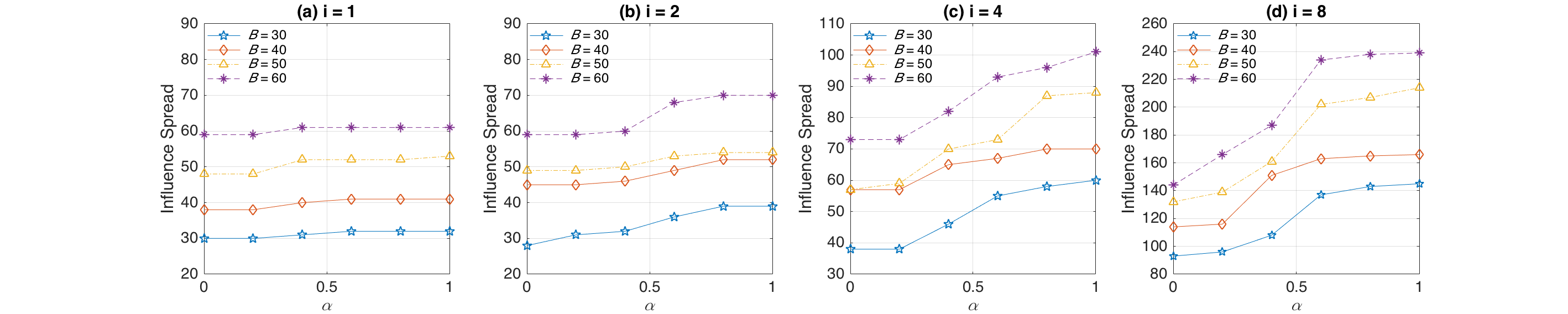
Figure 1: Influence spread vs. $\alpha$ on NetHEPT dataset under varying budget constraint.

We conduct extensive experiments on a real benchmark social networks: NetHEPT to examine the effectiveness and efficiency of $\alpha$-Greedy policy. We set the propagation probability of each directed edge randomly from $i\times\{0.01,0.001\}$ as in (Jung et al. 2012). We vary the value of $i$ and examine how it affects the quality of the solutions. Selecting the node with the largest marginal gain is #P-hard (Chen et al. 2010), and is typically approximated by numerous Monte Carlo simulations (Kempe et al. 2003). We adjust the value of control parameter $\alpha$ in range $[0,1]$.

Figure 1 shows the influence spread yielded by the proposed enhanced greedy policy on the NetHEPT dataset, as $\alpha$ ranges from $0$ to $1$ with a step of $0.2$. The $x$-axis corresponds to the value of the control parameter $\alpha$ and the $y$-axis holds the size of the influence spread achieved. We test the scenario with varying edge propagation probability distributions as discussed above. In particular, each edge is randomly assigned a propagation probability from $i\times\{0.01,0.001\}$. We adjust the value of $i$ from $1$ to $8$ and Figure 1(a)-(d) shows the comparison of the influence spread under $i=1$, $i=2$, $i=4$, $i=8$, respectively. In this set of experiments, the budget $B$ ranges from $30$ to $60$. The cost of each node is randomly assigned from $[1,10]$. As expected, a higher budget leads to a larger influence spread since the budget indirectly controls the number of seeds can be selected.

We observe that when $i$ takes a smaller value, take $i=1$ as an example, the advantage of performing adaptive seeding with partial feedback is not obvious since the improvement over influence spread does not increase much as $\alpha$ increases. The reason behind this is that a smaller $i$ indicates a lower probability for the edges to be alive, resulting in a lower uncertainty about the status of the edges. In this case observations gained from partial feedback may not help much since with high probability the estimation of influence spread based on sampling technique matches the real propagation. As shown in Figure 1, the advantage of taking adaptive seeding based on partial feedback becomes obvious as $i$ increases. We observe that when $i\geq 2$, a much larger influence spread can be achieved based on partial feedback ($\alpha>0$) compared to zero-feedback scenario ($\alpha=0$). For example, when $i=4$ with budget of $50$, while the influence spread based on zero-feedback leads to a size of $57$, the spread achieves a size of $87$ based on partial feedback ($\alpha=0.8$), a $52.6\%$ increase.

We also observe that a smaller $\alpha$ can lead to a significant improvement on influence spread with a higher edge propagation probability. For example, as shown in Figure 1, when $i=2$, a $10\%$ improvement can be achieved with $\alpha=0.6$. When $i=4$, a $20\%$ improvement can be achieved with $\alpha=0.4$. This implies that given a social graph with moderate edge propagation probability, it is worth to leverage the partial observation of diffusion realization, since adaptive seeding based on partial feedback leads to a significant improvement over the size of influence spread.

7 Conclusion

To the best of our knowledge, we are the first to systematically study the problem of influence maximization problem with partial feedback. Under independent cascade model, which is one of the most commonly used models in literature, we present two greedy algorithms with bounded approximation ratios.

References

• Badanidiyuru et al. (2016) Badanidiyuru, Ashwinkumar, Christos Papadimitriou, Aviad Rubinstein, Lior Seeman, Yaron Singer. 2016. Locally adaptive optimization: adaptive seeding for monotone submodular functions. Proceedings of the Twenty-Seventh Annual ACM-SIAM Symposium on Discrete Algorithms. SIAM, 414–429.
• Chen et al. (2013) Chen, Wei, Laks VS Lakshmanan, Carlos Castillo. 2013. Information and influence propagation in social networks. Synthesis Lectures on Data Management 5(4) 1–177.
• Chen et al. (2010) Chen, Wei, Chi Wang, Yajun Wang. 2010. Scalable influence maximization for prevalent viral marketing in large-scale social networks. Proceedings of the 16th ACM SIGKDD international conference on Knowledge discovery and data mining. ACM, 1029–1038.
• Chen et al. (2009) Chen, Wei, Yajun Wang, Siyu Yang. 2009. Efficient influence maximization in social networks. Proceedings of the 15th ACM SIGKDD international conference on Knowledge discovery and data mining. ACM, 199–208.
• Cohen et al. (2014) Cohen, Edith, Daniel Delling, Thomas Pajor, Renato F Werneck. 2014. Sketch-based influence maximization and computation: Scaling up with guarantees. Proceedings of the 23rd ACM International Conference on Conference on Information and Knowledge Management. ACM, 629–638.
• Domingos and Richardson (2001) Domingos, Pedro, Matt Richardson. 2001. Mining the network value of customers. Proceedings of the seventh ACM SIGKDD international conference on Knowledge discovery and data mining. ACM, 57–66.