Anisotropically Weighted and Nonholonomically Constrained Evolutions on Manifolds

Abstract

We present evolution equations for a family of paths that results from anisotropically weighting curve energies in non-linear statistics of manifold valued data. This situation arises when performing inference on data that have non-trivial covariance and are anisotropic distributed. The family can be interpreted as most probable paths for a driving semi-martingale that through stochastic development is mapped to the manifold. We discuss how the paths are projections of geodesics for a sub-Riemannian metric on the frame bundle of the manifold, and how the curvature of the underlying connection appears in the sub-Riemannian Hamilton-Jacobi equations. Evolution equations for both metric and cometric formulations of the sub-Riemannian metric are derived. We furthermore show how rank-deficient metrics can be mixed with an underlying Riemannian metric, and we relate the paths to geodesics and polynomials in Riemannian geometry. Examples from the family of paths are visualized on embedded surfaces, and we explore computational representations on finite dimensional landmark manifolds with geometry induced from right-invariant metrics on diffeomorphism groups.

1 Introduction

When manifold valued data have non-trivial covariance, i.e. when anisotropy asserts higher variance in some directions than others, non-zero curvature necessitates special care when generalizing Euclidean space normal distributions to manifold valued distributions: In the Euclidean situation, normal distributions can be seen as transition distributions of diffusion processes but, on the manifold, holonomy makes transport of covariance path-dependent in the presence of curvature preventing a global notion of spatially constant covariance matrix. To handle this, in the diffusion PCA framework [Som14] and with the class of anisotropic normal distributions on manifolds defined in [Som15, SS16], data on non-linear manifolds are modelled as being distributed according to transition distributions of anisotropic diffusion processes that are mapped from Euclidean space to the manifold by stochastic development (see [Hsu02]). The construction is connected to a non bracket-generating sub-Riemannian metric on the bundle of linear frames of the manifold, the frame bundle, and the requirement that covariance stays covariantly constant gives a nonholonomically constrained system.

Velocity vectors and geodesic distances are conventionally used for estimation and statistics in Riemannian manifolds, for example for estimating the Frechét mean [Fr48], for Principal Geodesic Analysis [FLPJ04], and for tangent space statistics [VMYT04]. In contrast to this, anisotropy as modelled with anisotropic normal distributions makes a distance for a sub-Riemannian metric the natural vehicle for estimation and statistics. This metric naturally accounts for anisotropy in a similar way as the precision matrix weights the inner product in the negative log-likelihood of a Euclidean normal distribution. The connection between the weighted distance and statistics of manifold valued data was presented in [Som15], and the underlying sub-Riemannian and fiber-bundle geometry together with properties of the generated densities was further explored in [SS16]. The fundamental idea is to perform statistics on manifolds by maximum likelihood (ML) instead of parametric constructions that use e.g. approximating geodesic subspaces: by defining natural families of probability distributions, in this case using diffusion processes, ML parameter estimates gives a coherent way to statistically model non-linear data. The anisotropically weighted distance and the resulting family of extremal paths arises in this situation when the diffusion processes have non-isotropic covariance, i.e. when the distribution is not generated from a standard Brownian motion.

In this paper, we focus on the family of most probable paths for the semi-martingales that drives the stochastic development and in turn the manifold valued anisotropic stochastic processes. These paths extremize the anisotropically weighted action functional. We present derivations of evolution equations for the paths from different viewpoints, and we discuss the role of frames as representing either metrics or cometrics. In the derivation, we explicitly see the influence of the connection and its curvature. We then turn to the relation between the sub-Riemannian metric and the Sasaki-Mok metric on the frame bundle, and we develop a construction that allows the sub-Riemannian metric to be defined as a sum of a rank-deficient generator and an underlying Riemannian metric. Finally, we relate the paths to geodesics and polynomials in Riemannian geometry, and we explore computational representations on different manifolds including a specific case, the finite dimensional manifolds arising in the LDDMM [You10] landmark matching problem. The paper ends with a discussion concerning statistical implications, open questions, and concluding remarks.

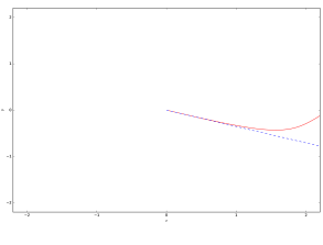
Figure 1: (left) A most probable path (MPP) for a driving Euclidean Brownian motion on an ellipsoid. The gray ellipsis over the starting point (red dot) indicates the covariance of the anisotropic diffusion. A frame $u_{t}$ (black/gray vectors) representing the square root covariance is parallel transported along the curve enabling the anisotropic weighting with the precision matrix in the action functional. With isotropic covariance, normal MPPs are Riemannian geodesics. In general situations such as the displayed anisotropic case, the family of MPPs is much larger. (right) The corresponding anti-development in $\mathbb{R}^{2}$ (red line) of the MPP. Compare with the anti-development of a Riemannian geodesic with same initial velocity (blue dotted line). The frames $u_{t}\in\mathrm{GL}(\mathbb{R}^{2},T_{x_{t}}M)$ provide local frame coordinates for each time $t$.

1.1 Background

Generalizing common statistical tools for performing inference on Euclidean space data to manifold valued data has been the subject of extensive work, see e.g. [Pen06]. Perhaps most fundamental is the notion of Frechét or Karcher means [Fr48, Kar77] defined as minimizers of the square Riemannian distance. Generalizations of the Euclidean Principal Component Analysis (PCA) procedure to manifolds are particularly relevant for data exhibiting anisotropy. Approaches include Principal Geodesic Analysis (PGA, [FLPJ04]), Geodesic PCA (GPCA, [HHM10]), Principal Nested Spheres (PNS, [JDM12]), Barycentric Subspace Analysis (BSA, [Pen15]), and Horizontal Component Analysis (HCA, [Som13]). Common to these constructions are explicit representations of approximating low-dimensional subspaces. The fundamental challenge is here that the notion of Euclidean linear subspace on which PCA relies has no direct analogue in non-linear spaces.

A different approach taken by Diffusion PCA (DPCA, [Som14, Som15]) and Probabilistic PGA [ZF13] is to base the PCA problem on a maximum likelihood fit of normal distributions to data. In Euclidean space, this approach was first introduced with Probabilistic PCA [TB99]. In DPCA, the process of stochastic development [Hsu02] is used to define a class of anisotropic distributions that generalizes the family of Euclidean space normal distributions to the manifold context. DPCA is then a simple maximum likelihood fit in this family of distributions mimicking the Euclidean Probabilistic PCA. The approach transfers the geometric complexities of defining subspaces common in the approaches listed above to the problem of defining a geometrically natural notion of normal distributions.

Figure 2: (left) Normal distributions $u\mathcal{N}(0,\mathrm{Id})$ in the tangent space $T_{x_{0}}M$ with covariance $uu^{T}$ (blue ellipsis) can be mapped to the manifold by applying the exponential map $\mathrm{Exp}_{x_{0}}$ to sampled vectors $v\in T_{x_{0}}M$ (red vectors). This effectively linearises the geometry around $x_{0}$. (right) The stochastic development map $\varphi_{u}$ maps $\mathbb{R}^{d}$ valued paths $w_{t}$ to $M$ by transporting the covariance in each step (blue ellipses) giving a covariance $u_{t}$ along the entire sample path. The approach does not linearise around a single point. Holonomy of the connection implies that the covariance “rotates” around closed loops, an effect which can be illustrated by continuing the transport along the loop created by the dashed path. The anisotropic metric $g_{FM}$ weights step lengths by the transported covariance at each time $t$.

In Euclidean space, squared distances $\|x-x_{0}\|^{2}$ between observations $x$ and the mean $x_{0}$ are affinely related to the negative log-likelihood of a normal distribution $\mathcal{N}(x_{0},\mathrm{Id})$. This makes an ML fit of the mean such as performed in Probabilistic PCA equivalent to minimizing squared distances. On a manifold, distances $d_{g}(x,x_{0})^{2}$ coming from a Riemannian metric $g$ are equivalent to tangent space distances $\|\mathrm{Log}_{x_{0}}x\|^{2}$ when mapping data from $M$ to $T_{x_{0}}M$ using the inverse exponential map $\mathrm{Log}_{x_{0}}$. Assuming $\mathrm{Log}_{x_{0}}x$ are distributed according to a normal distribution in the linear space $T_{x_{0}}M$, this restores the equivalence with a maximum likelihood fit. Let $\{e_{1},\ldots,e_{d}\}$ be the standard basis for $\mathbb{R}^{d}$. If $u:\mathbb{R}^{d}\rightarrow T_{x_{0}}M$ is a linear invertible map with $ue_{1},\ldots,ue_{d}$ orthonormal with respect to $g$, the normal distribution in $T_{x_{0}}M$ can be defined as $u\mathcal{N}(0,\mathrm{Id})$, see Figure 2.

The map $u$ can be represented as a point in the frame bundle $FM$ of $M$. When the orthonormal requirement on $u$ is relaxed so that $u\mathcal{N}(0,\mathrm{Id})$ is a normal distribution in $T_{x_{0}}M$ with anisotropic covariance, the negative log-likelihood in $T_{x_{0}}M$ is related to $(u^{-1}\mathrm{Log}_{x_{0}}x)^{T}(u^{-1}\mathrm{Log}_{x_{0}}x)$ in the same way as the precision matrix $\Sigma^{-1}$ is related to the negative log-likelihood $(x-x_{0})^{T}\Sigma^{-1}(x-x_{0})$ in Euclidean space. The distance is thus weighted by the anisotropy of $u$, and $u$ can be interpreted as a square root covariance matrix $\Sigma^{1/2}$.

However, the above approach does not specify how $u$ changes when moving away from the base point $x_{0}$. The use of $\mathrm{Log}_{x_{0}}x$ effectively linearises the geometry around $x_{0}$ but a geometrically natural way to relate $u$ at points nearby to $x_{0}$ will be to parallel transport it, equivalently specify that $u$ when transported does not change as measured from the curved geometry. This constraint is nonholonomic and it implies that any path from $x_{0}$ to $x$ carries with it a parallel transport of $u$ lifting paths from $M$ to paths in the frame bundle $FM$. It therefore becomes natural to equip $FM$ with a form of metric that encodes the anisotropy represented by $u$. The result is the sub-Riemannian metric on $FM$ defined below that weights infinitesimal movements on $M$ using the parallel transport of the frame $u$. Optimal paths for this metric are sub-Riemannian geodesics giving the family of most probable paths for the driving process that this paper concerns. Figure 1 shows one such path for an anisotropic normal distribution with $M$ an ellipsoid embedded in $\mathbb{R}^{3}$.

2 Frame Bundles, Stochastic Development, and Anisotropic Diffusions

Let $M$ be a finite dimensional manifold of dimension $d$ with connection ${\mathcal{C}}$, and let $x_{0}$ be a fixed point in $M$. When a Riemannian metric is present and ${\mathcal{C}}$ is its Levi-Civita connection, we denote the metric $g_{R}$. For a given interval $[0,T]$, we let $W(M)$ denote the Wiener space of continuous paths in $M$ starting at $x_{0}$. Similarly, $W(\mathbb{R}^{d})$ is the Wiener space of paths in $\mathbb{R}^{d}$. We let $H(\mathbb{R}^{d})$ denote the subspace of $W(\mathbb{R}^{d})$ of finite energy paths.

Let now $u=(u_{1},\ldots,u_{d})$ be a frame for $T_{x}M$, $x\in M$, i.e. $u_{1},\ldots,u_{d}$ is an ordered set of linearly independent vectors in $T_{x}M$ with $\mathrm{span}\{u_{1},\ldots,u_{d}\}=T_{x}M$. We can regard the frame as an isomorphism $u:\mathbb{R}^{d}\to T_{x}M$ with $u(e_{i})=u_{i}$ where $e_{1},\ldots,e_{d}$ denotes the standard basis in $\mathbb{R}^{d}$. Stochastic development, see e.g. [Hsu02], provides an invertible map $\varphi_{u}$ from $W(\mathbb{R}^{d})$ to $W(M)$. Through $\varphi_{u}$, Euclidean semi-martingales map to stochastic processes on $M$. When $M$ is Riemannian and $u$ orthonormal, the result is the Eells-Elworthy-Malliavin construction of Brownian motion [Elw88]. We here outline the geometry behind development, stochastic development, the connection and curvature focusing in particular on frame bundle geometry.

2.1 The Frame Bundle

For each point $x\in M$, let $F_{x}M$ be the set of frames for $T_{x}M$, i.e. the set of ordered bases for $T_{x}M$. The set $\{F_{x}M\}_{x\in M}$ can be given a natural differential structure as a fiber bundle on $M$ called the frame bundle $FM$. It can equivalently be defined as the principal bundle $\mathrm{GL}(\mathbb{R}^{d},TM)$. We let the map $\pi:FM\rightarrow M$ denote the canonical projection. The kernel of $\pi_{*}:TFM\rightarrow TM$ is the subbundle of $TFM$ that consists of vectors tangent to the fibers $\pi^{-1}(x)$. It is denoted the vertical subspace $VFM$. We will often work in a local trivialization $u=(x,u_{1},\ldots,u_{d})\in FM$ where $x=\pi(u)\in M$ denotes the base point and for each $i=1,\ldots,d$, $u_{i}\in T_{x}M$ is the $i$th frame vector. For $v\in T_{x}M$ and $u\in FM$ with $\pi(u)=x$, the vector $u^{-1}v\in\mathbb{R}^{d}$ expresses $v$ in components in terms of the frame $u$. We will denote the vector $u^{-1}v$ frame coordinates of $v$.

For a differentiable curve $x_{t}$ in $M$ with $x=x_{0}$, a frame $u$ for $T_{x_{0}}M$ can be parallel transported along $x_{t}$ by parallel transporting each vector in the frame thus giving a path $u_{t}\in FM$. Such paths are called horizontal and have zero acceleration in the sense ${\mathcal{C}}(\dot{u}_{i,t})=0$. For each $x\in M$, their derivatives form a $d$-dimensional subspace of the $d+d^{2}$-dimensional tangent space $T_{u}FM$. This horizontal subspace $HFM$ and the vertical subspace $VFM$ together split the tangent bundle of $FM$, i.e. $TFM=HFM\oplus VFM$. The split induces a map $\pi_{*}:HFM\rightarrow TM$, see Figure 3. For fixed $u\in FM$, the restriction $\pi_{*}|_{H_{u}FM}:H_{u}FM\rightarrow T_{x}M$ is an isomorphism. Its inverse is called the horizontal lift and denoted $h_{u}$ in the following. Using $h_{u}$, horizontal vector fields $H_{e}$ on $FM$ are defined for vectors $e\in\mathbb{R}^{d}$ by $H_{e}(u)=h_{u}(ue)$. In particular, the standard basis $(e_{1},\ldots,e_{d})$ on $\mathbb{R}^{d}$ gives $d$ globally defined horizontal vector fields $H_{i}\in HFM$, $i=1,\ldots,d$ by $H_{i}=H_{e_{i}}$. Intuitively, the fields $H_{i}(u)$ model infinitesimal transformations in $M$ of $x_{0}$ in direction $u_{i}=ue_{i}$ with corresponding infinitesimal parallel transport of the vectors $u_{1},\ldots,u_{d}$ of the frame along the direction $u_{i}$. A horizontal lift of a differentiable curve $x_{t}\in M$ is a curve in $FM$ tangent to $HFM$ that projects to $x_{t}$. Horizontal lifts are unique up to the choice of initial frame $u_{0}$.

2.2 Development and Stochastic Development

Let $x_{t}$ be a differentiable curve on $M$ and $u_{t}$ a horizontal lift. If $s_{t}$ is a curve in $\mathbb{R}^{d}$ with components $s_{t}^{i}$ such that $\dot{x}_{t}=H_{i}(u)s_{t}^{i}$, $x_{t}$ is said to be a development of $s_{t}$. Correspondingly, $s_{t}$ is the anti-development of $x_{t}$. For each $t$, the vector $s_{t}$ contains frame coordinates of $\dot{x}_{t}$ as defined above. Similarly, let $W_{t}$ be an $\mathbb{R}^{d}$ valued Brownian motion so that sample paths $W_{t}(\omega)\in W(\mathbb{R}^{d})$. A solution to the stochastic differential equation $dU_{t}=\sum_{i=1}^{d}H_{i}(U_{t})\circ dW^{i}_{t}$ in $FM$ is called a stochastic development of $W_{t}$ in $FM$. The solution projects to a stochastic development $X_{t}=\pi(U_{t})$ in $M$. We call the process $W_{t}$ in $\mathbb{R}^{d}$, that through $\varphi$ maps to $X_{t}$, the driving process of $X_{t}$. Let $\varphi_{u}:W(\mathbb{R}^{d})\rightarrow W(M)$ be the map that for fixed $u$ sends a path in $\mathbb{R}^{d}$ to its development on $M$. Its inverse $\varphi_{u}^{-1}$ is the anti-development in $\mathbb{R}^{d}$ of paths on $M$ given $u$.

Equivalent to the fact that normal distributions $\mathcal{N}(0,\Sigma)$ in $\mathbb{R}^{d}$ can be obtained as the transition distributions of diffusion processes $\Sigma^{1/2}W_{t}$ stopped at time $t=1$, a general class of distributions on the manifold $M$ can be defined by stochastic development of processes $W_{t}$ resulting in $M$-valued random variables $X=X_{1}$. This family of distributions on $M$ introduced in [Som15] is denoted anisotropic normal distributions. The stochastic development by construction ensures that $U_{t}$ is horizontal, and the frames are thus parallel transported along the stochastic displacements. The effect is that the frames stay covariantly constant thus resembling the Euclidean situation where $\Sigma^{1/2}$ is spatially constant and therefore does not change as $W_{t}$ evolves. Thus, as further discussed in Section 3.2, the covariance is kept constant at each of the infinitesimal stochastic displacements. The existence of a smooth density for the target process $X_{t}$ and small time asymptotics are discussed in [SS16].

Figure 3: Relations between the manifold, frame bundle, the horizontal distribution $HFM$, the vertical bundle $VFM$, a Riemannian metric $g_{R}$ and the sub-Riemannian metric $g_{FM}$ defined below. The connection ${\mathcal{C}}$ provides the splitting $TFM=HFM\oplus VFM$. The restrictions $\pi_{*}|_{H_{u}M}$ are invertible maps $H_{u}M\rightarrow T_{\pi(u)}M$ with inverse $h_{u}$, the horizontal lift. Correspondingly, the vertical bundle $VFM$ is isomorphic to the trivial bundle $FM\times\mathfrak{gl}(n)$. The metric $g_{FM}:T^{*}FM\rightarrow TFM$ has image in the subspace $HFM$.

Stochastic development gives a map $\int_{\mathrm{Diff}}:FM\rightarrow\mathrm{Prob}(M)$ to the space of probability distributions on $M$. For each point $u\in FM$, the map sends a Brownian motion in $\mathbb{R}^{d}$ to a distribution $\mu_{u}$ by stochastic development of the process $U_{t}$ in $FM$ starting at $u$ and letting $\mu_{u}$ be the distribution of $X=\pi(U_{1})$. The pair $(x,u)$, $x=\pi(u)$ is analogous to the parameters $(\mu,\Sigma)$ for a Euclidean normal distribution: The point $x\in M$ represents the starting point of the diffusion, and the frame $u$ represents a square root $\Sigma^{1/2}$ of the covariance $\Sigma$. In the general situation where $\mu_{u}$ has smooth density, the construction can be used to fit the parameters $u$ to data by maximum likelihood. As an example, Diffusion PCA fits distributions obtained through $\int_{\mathrm{Diff}}$ by maximum likelihood to observed samples in $M$, i.e. it optimizes for the most likely parameters $u=(x,u_{1},\ldots,u_{d})$ for the anisotropic diffusion process giving a fit to the data of the manifold generalization of the Euclidean normal distribution.

2.3 Adapted Coordinates

For concrete expressions of the geometric constructions related to frame bundles and for computational purposes, it is useful to apply coordinates that are adapted to the horizontal bundle $HFM$ and the vertical bundle $VFM$ together with their duals $H^{*}FM$ and $V^{*}FM$. The notation below follows the notation used in for example [Mok78]. Let $z=(u,\xi)$ be a local trivialization of $T^{*}FM$, and let $(x^{i},u^{i}_{\alpha})$ be coordinates on $FM$ with $u^{i}_{\alpha}$ satisfying $u_{\alpha}=u^{i}_{\alpha}\partial_{x^{i}}$ for each $\alpha=1,\ldots,d$.

To find a basis that is adapted to the horizontal distribution, define the $d$ linearly independent vector fields $D_{j}=\partial_{x^{j}}-\Gamma^{h_{\gamma}}_{j}\partial_{u^{h}_{\gamma}}$ where $\Gamma^{h_{\gamma}}_{j}=\Gamma\indices{{}^{h}_{ji}}u^{i}_{\gamma}$ is the contraction of the Christoffel symbols $\Gamma\indices{{}^{h}_{ij}}$ for the connection ${\mathcal{C}}$ with $u_{\alpha}^{i}$. We denote this adapted frame $D$. The vertical distribution is correspondingly spanned by $D_{j_{\beta}}=\partial_{u^{j}_{\beta}}$. The vectors $D^{h}=dx^{h},$ and $D^{h_{\gamma}}=\Gamma^{h_{\gamma}}_{j}dx^{j}+du^{h}_{\gamma}$ constitutes a dual coframe $D^{*}$. The map $\pi_{*}:HFM\rightarrow TM$ is in coordinates of the adapted frame $\pi_{*}(w^{j}D_{j})=w^{j}\partial_{x^{j}}$. Correspondingly, the horizontal lift $h_{u}$ is $h_{u}(w^{j}\partial_{x^{j}})=w^{j}D_{j}$. The map $u:\mathbb{R}^{d}\rightarrow T_{x}M$ is given by the matrix $[u^{i}_{\alpha}]$ so that $uv=u^{i}_{\alpha}v^{\alpha}\partial_{x^{i}}=u_{\alpha}v^{\alpha}$.

Switching between standard coordinates and the adapted frame and coframes can be expressed in terms of the component matrices $A$ below of the frame and coframe induced by the coordinates $(x^{i},u_{\alpha}^{i})$ and the adapted frame $D$ and coframe $D^{*}$. We have

$$\,{}_{(\partial_{x^{i}},\partial_{u_{\alpha}^{i}})}A_{D}=\begin{bmatrix}I&0\\ -\Gamma&I\end{bmatrix}\mbox{ with inverse }\,_{D}A_{(\partial_{x^{i}},\partial_{u_{\alpha}^{i}})}=\begin{bmatrix}I&0\\ \Gamma&I\end{bmatrix}$$

writing $\Gamma$ for the matrix $[\Gamma^{h_{\gamma}}_{j}]$. Similarly, the component matrices of the dual frame $D^{*}$ are

$$\,{}_{(\partial_{x^{i}},\partial_{u_{\alpha}^{i}})^{*}}A_{D^{*}}=\begin{bmatrix}I&\Gamma^{T}\\ 0&I\end{bmatrix}\mbox{ and }\,_{D^{*}}A_{(\partial_{x^{i}},\partial_{u_{\alpha}^{i}})^{*}}=\begin{bmatrix}I&-\Gamma^{T}\\ 0&I\end{bmatrix}\ .$$

2.4 Connection and Curvature

The $TM$ valued connection ${\mathcal{C}}:TM\times TM\rightarrow TM$ lifts to a principal connection $TFM\times TFM\rightarrow VFM$ on the principal bundle $FM$. ${\mathcal{C}}$ can then be identified with the $\mathfrak{gl}(n)$-valued connection form $\omega$ on $TFM$. The identification occurs by the isomorphism $\psi$ between $FM\times\mathfrak{gl}(n)$ and $VFM$ given by $\psi(u,v)=\tfrac{d}{dt}u\exp(tv)|_{t=0}$, see e.g. [Tau11, KSM93].

The map $\psi$ is equivariant with respect to the $\mathrm{GL}(n)$ action $g\mapsto ug^{-1}$ on $FM$. In order to explicitly see the connection between the usual covariant derivative $\nabla:\Gamma(TM)\times\Gamma(TM)\rightarrow\Gamma(TM)$ on $M$ determined by ${\mathcal{C}}$ and ${\mathcal{C}}$ regarded as a connection on the principal bundle $FM$, following [Tau11], we let $s:M\rightarrow TM$ be a local vector field on $M$, equivalently $s\in\Gamma(TM)$ is a local section of $TM$. $s$ determines a map $s^{FM}:FM\rightarrow\mathbb{R}^{d}$ by $s^{FM}(u)=u^{-1}s(\pi(u))$, i.e. it gives the coordinates of $s(x)$ in the frame $u$ at $x$. The pushforward $(s^{FM})_{*}:TFM\rightarrow\mathbb{R}^{d}$ has in its $i$th component the exterior derivative $d(s^{FM})^{i}$. Let now $w(x)$ be a local section of $FM$. The composition $w\circ(s^{FM})_{*}\circ h_{w}:TM\rightarrow TM$ is identical to the covariant derivative $\nabla_{\cdot}s:TM\rightarrow TM$. The construction is independent of the choice of $w$ because of the $\mathrm{GL}(n)$-equivariance of $s^{FM}$. The connection form $\omega$ can be expressed as the matrix $(s_{1}^{FM}\circ h_{w},\ldots,s_{d}^{FM}\circ h_{w})$ when letting $s_{i}^{FM}(u)=e_{i}$.

The identification becomes particularly simple if the covariant derivative is taken along a curve $x_{t}$ on which $w_{t}$ is the horizontal lift. In this case, we can let $s_{t}=w_{t,i}s^{i}_{t}$. Then $s^{FM}(w_{t})=(s^{1}_{t},\ldots,s^{d}_{t})^{T}$ and

$$w_{t}^{-1}\nabla_{\dot{x}_{t}}s=(s^{F}M)_{*}(h_{w_{t}}(\dot{x}_{t}))=\tfrac{d}{dt}(s^{1}_{t},\ldots,s^{d}_{t})^{T}\ ,$$ (1)

i.e. the covariant derivative takes the form of the standard derivative applied to the frame coordinates $s^{i}_{t}$.

The curvature tensor $R\in\mathcal{T}^{3}_{1}(M)$ gives the $\mathfrak{gl}(n)$-valued curvature form $\Omega:TFM\times TFM\rightarrow\mathfrak{gl}(n)$ on $TFM$ by

$$\Omega(v_{u},w_{u})=u^{-1}R(\pi_{*}(v_{u}),\pi_{*}(w_{u}))u\ ,\ v_{u},w_{v}\in TFM\ .$$

Note that $\Omega(v_{u},w_{u})=\Omega(h_{u}(\pi_{*}(v_{u})),h_{u}(\pi_{*}(w_{u})))$ which we can use to write the curvature $R$ as the $\mathfrak{gl}(n)$-valued map $R_{u}:T^{2}(T_{\pi(u)}M)\rightarrow\mathfrak{gl}(n)$, $(v,w)\mapsto\Omega(h_{u}(\pi_{*}(v_{u})),h_{u}(\pi_{*}(w_{u})))$ for fixed $u$. In coordinates, the curvature is

$$R\indices{{}_{ijk}^{s}}=\Gamma\indices{{}^{l}_{ik}}\Gamma\indices{{}^{s}_{jl}}-\Gamma\indices{{}^{l}_{jk}}\Gamma\indices{{}^{s}_{il}}+\Gamma\indices{{}^{s}_{ik;j}}-\Gamma\indices{{}^{s}_{jk;i}}$$

where $\Gamma\indices{{}^{s}_{ik;j}}=\partial_{x^{j}}\Gamma\indices{{}^{s}_{ik}}$.

Let $x_{t,s}$ be a family of paths in $M$ and let $u_{t,s}\in\pi^{-1}(x_{t,s})$ be horizontal lifts of $x_{t,s}$ for each fixed $s$. Write $\dot{x}_{t,s}=\partial_{t}x_{t,s}$ and $\dot{u}_{t,s}=\partial_{t}u_{t,s}$. The $s$-derivative of $u_{t,s}$ can be regarded a pushforward of the horizontal lift and is the curve in $TFM$

$$\begin{split}\partial_{s}u_{t,s}&=\psi\big{(}u_{t,s},\psi_{u_{0,s}}^{-1}({\mathcal{C}}(\partial_{s}u_{0,s}))+\int_{0}^{s}\Omega(\dot{u}_{r,s},\partial_{s}u_{r,s})dr\big{)}+h_{u_{t,s}}(\partial_{s}x_{t,s})\\ &=\psi\big{(}u_{t,s},\psi_{0,s}^{-1}({\mathcal{C}}(\partial_{s}u_{0,s}))+\int_{0}^{s}R_{u_{r,s}}(\dot{x}_{r,s},\partial_{s}x_{r,s})dr\big{)}+h_{u_{t,s}}(\partial_{s}x_{t,s})\ .\end{split}$$ (2)

This follows from the structure equation $d\omega=-\omega\wedge\omega+\Omega$, see e.g. [AD99]. Note that the curve depends on the vertical variation ${\mathcal{C}}(\partial_{s}u_{0,s})$ at only one point along the curve. The remaining terms depend on the horizontal variation or, equivalently, $\partial_{s}x_{t,s}$. The $t$-derivative of $\partial_{s}u_{t,s}$ is the curve in $TTFM$ satisfying

$$\begin{split}\partial_{s}h_{u_{t,s}}(\dot{x}_{t,s})&=\psi\big{(}u_{t,s},R_{u_{t,s}}(\dot{x}_{t,s},\partial_{s}x_{t,s})\big{)}+\partial_{t}\psi\big{(}u_{t,s},\psi_{0,s}^{-1}({\mathcal{C}}(\partial_{s}u_{0,s}))\big{)}+\partial_{t}\big{(}h_{u_{t,s}}(\partial_{s}x_{t,s})\big{)}\\ &=\psi\big{(}u_{t,s},R_{u_{t,s}}(\dot{x}_{t,s},\partial_{s}x_{t,s})\big{)}+\partial_{t}\psi\big{(}u_{t,s},\psi_{0,s}^{-1}({\mathcal{C}}(\partial_{s}u_{0,s}))\big{)}\\ &\qquad+h_{u_{t,s}}(\partial_{t}\partial_{s}x_{t,s})+(\partial_{t}h_{u_{t,s}})(\partial_{s}x_{t,s})\ .\end{split}$$ (3)

Here, the first and third term in the last expression are identified with elements of $T_{\partial_{s}u_{t,s}}TFM$ by the natural mapping $T_{u_{t,s}}FM\rightarrow T_{\partial_{s}u_{t,s}}TFM$. When ${\mathcal{C}}(\partial_{s}u_{0,s})$ is zero, the relation reflects the property that the curvature arise when computing brackets between horizontal vector fields. Note that the first term of (3) has values in $VFM$ while the third term has values in $HFM$.

3 The Anisotropically Weighted Metric

For a Euclidean driftless diffusion process with spatially constant stochastic generator $\Sigma$, the log-probability of a sample path can formally be written

$$\ln\tilde{p}_{\Sigma}(x_{t})\propto-\int_{0}^{1}\|\dot{x}_{t}\|_{\Sigma}^{2}dt+c_{\Sigma}$$ (4)

with the norm $\|\cdot\|_{\Sigma}$ given by the inner product $\left<v,w\right>_{\Sigma}=\left<\Sigma^{-1/2}v,\Sigma^{-1/2}w\right>=v\Sigma^{-1}w$, i.e. the inner product weighted by the precision matrix $\Sigma^{-1}$. Though only formal as the sample paths are almost surely nowhere differentiable, the interpretation can be given a precise meaning by taking limits of piecewise linear curves [AD99]. Turning to the manifold situation with the processes mapped to $M$ by stochastic development, the probability of observing a differentiable path can either be given a precise meaning in the manifold by taking limits of small tubes around the curve, or in $\mathbb{R}^{d}$ by considering infinitesimal tubes around the anti-development of the curves. With the former formulation, a scalar curvature correction term must be added to (4) giving the Onsager-Machlup function [FK82]. The latter formulation corresponds to defining a notion of path density for the driving $\mathbb{R}^{d}$-valued process $W_{t}$. When $M$ is Riemannian and $\Sigma$ unitary, taking the maximum of (4) gives geodesics as most probable paths for the driving process.

Let now $u_{t}$ be a path in $FM$ and choose a local trivialization $u_{t}=(x_{t},u_{1,t},\ldots,u_{d,t})$ such that the matrix $[u_{\alpha,t}^{i}]$ represents the square root covariance matrix $\Sigma^{1/2}$ at $x_{t}$. Since $u_{t}$ being a frame defines an invertible map $\mathbb{R}^{d}\rightarrow T_{x_{t}}M$, the norm $\|\cdot\|_{\Sigma}$ above has a direct analogue in the norm $\|\cdot\|_{u_{t}}$ defined by the inner product

$$\left<v,w\right>_{u_{t}}=\left<u_{t}^{-1}v,u_{t}^{-1}w\right>_{\mathbb{R}^{d}}$$ (5)

for vectors $v,w\in T_{x_{t}}M$. The transport of the frame along paths in effect defines a transport of inner product along sample paths: The paths carry with them the inner product weighted by the precision matrix which in turn is a transport of the square root covariance $u_{0}$ at $x_{0}$.

The inner product can equivalently be defined as a metric $g_{u}:T^{*}_{x}M\rightarrow T_{x}M$. Again using that $u$ can be considered a map $\mathbb{R}^{d}\rightarrow T_{x}M$, $g_{u}$ is defined by $\xi\mapsto u_{(}(\xi\circ u)^{\sharp})$ where $\sharp$ is the standard identification $(\mathbb{R}^{d})^{*}\rightarrow\mathbb{R}^{d}$. The sequence of mappings defining $g_{u}$ is illustrated below:

$$\begin{matrix}T^{*}_{x}M&\rightarrow&(\mathbb{R}^{d})^{*}&\rightarrow&\mathbb{R}^{d}&\rightarrow&T_{x}M\\ \xi\quad&\mapsto&\quad\xi\circ u\quad&\mapsto&\quad(\xi\circ u)^{\sharp}\quad&\mapsto&\quad u(\xi\circ u)^{\sharp}\ .\end{matrix}$$ (6)

This definition uses the $\mathbb{R}^{d}$ inner product in the definition of $\sharp$. Its inverse gives the cometric $g_{u}^{-1}:T_{x}M\rightarrow T_{x}^{*}M$, i.e. $v\mapsto(u^{-1}v)^{\flat}\circ u^{-1}$.

$$\begin{matrix}T_{x}M&\rightarrow&\mathbb{R}^{d}&\rightarrow&(\mathbb{R}^{d})^{*}&\rightarrow&T_{x}^{*}M\\ v&\mapsto&u^{-1}v&\mapsto&(u^{-1})^{\flat}&\mapsto&(u^{-1})^{\flat}\circ u^{-1}\ .\end{matrix}$$ (7)

3.1 Sub-Riemannian Metric on the Horizontal Distribution

We now lift the path-dependent metric defined above to a sub-Riemannian metric on $HFM$. For any $w,\tilde{w}\in H_{u}FM$, the lift of (5) by $\pi_{*}$ is the inner product

$$\left<w,\tilde{w}\right>=\left<u^{-1}\pi_{*}w,u^{-1}\pi_{*}\tilde{w}\right>_{\mathbb{R}^{d}}\ .$$

The inner product induces a sub-Riemannian metric $g_{FM}:TFM^{*}\rightarrow HFM\subset TFM$ by

$$\left<w,g_{FM}(\xi)\right>=(\xi|w)\ ,\ \forall w\in H_{u}FM$$ (8)

with $(\xi|w)$ denoting the evaluation $\xi(w)$ for the covector $\xi\in T^{*}FM$. The metric $g_{FM}$ gives $FM$ a non bracket-generating sub-Riemannian structure [Str86] on $FM$, see also Figure 3. It is equivalent to the lift

$$\xi\mapsto h_{u}(g_{u}(\xi\circ h_{u}))\ ,\ \xi\in T_{u}FM$$ (9)

of the metric $g_{u}$ above. In frame coordinates, the metric takes the form

$$u^{-1}\pi_{*}g_{FM}(\xi)=\begin{pmatrix}\xi(H_{1}(u))\\ \vdots\\ \xi(H_{d}(u))\end{pmatrix}\ .$$ (10)

In terms of the adapted coordinates for $TFM$ described in Section 2.3, with $w=w^{j}D_{j}$ and $\tilde{w}=\tilde{w}^{j}D_{j}$, we have

$$\left<w,\tilde{w}\right> =\left<w^{i}D_{i},\tilde{w}^{j}D_{j}\right>=\left<u^{-1}w^{i}\partial_{x^{i}},u^{-1}\tilde{w}^{j}\partial_{x^{j}}\right>$$

$$=\left<w^{i}u^{\alpha}_{i},\tilde{w}^{j}u^{\alpha}_{j}\right>_{\mathbb{R}^{d}}=\delta_{\alpha\beta}w^{i}u^{\alpha}_{i}\tilde{w}^{j}u^{\beta}_{j}=W_{ij}w^{i}\tilde{w}^{j}$$

where $[u^{\alpha}_{i}]$ is the inverse of $[u^{i}_{\alpha}]$ and $W_{ij}=\delta_{\alpha\beta}u^{\alpha}_{i}u^{\beta}_{j}$. Define now $W^{kl}=\delta^{\alpha\beta}u^{k}_{\alpha}u^{l}_{\beta}$ so that $W^{ir}W_{rj}=\delta^{i}_{j}$ and $W_{ir}W^{rj}=\delta_{i}^{j}$. We can then write the metric $g_{FM}$ directly as

$$g_{FM}(\xi_{h}D^{h}+\xi_{h_{\gamma}}D^{h_{\gamma}})=W^{ih}\xi_{h}D_{i}\ ,$$ (11)

because $\left<w,g_{FM}(\xi)\right>=\left<w,W^{jh}\xi_{h}D_{j}\right>=W_{ij}w^{i}W^{jh}\xi_{h}=w^{i}\xi_{i}=\xi_{h}D^{h}(w^{j}D_{j})=\xi(w)$. One clearly recognizes the dependence on the horizontal $H^{*}FM$ part of $T^{*}FM$ only and the fact that $g_{FM}$ has image in $HFM$. The sub-Riemannian energy of an a.e. horizontal path $u_{t}$ is

$$l_{FM}(u_{t})=\int g_{FM}(\dot{u}_{t},\dot{u}_{t})dt\ ,$$

i.e., the line element is $ds^{2}=W_{ij}D^{i}D^{j}$ in adapted coordinates. The corresponding distance is given by

$$d_{FM}(u_{1},u_{2})=\inf\{l_{FM}(\gamma)\mid\gamma(0)=u_{1},\gamma(1)=u_{2}\}\ .$$

If we wish to express $g_{FM}$ in canonical coordinates on $T^{*}FM$, we can switch between the adapted frame and the coordinates $(x^{i},u_{\alpha}^{i},\xi^{i},\xi_{\alpha}^{i})$. From (11), $g_{FM}$ has $D,D^{*}$ components

$$\,{}_{D}g_{FM,D^{*}}=\begin{bmatrix}W^{-1}&0\\ 0&0\end{bmatrix}\ .$$

Therefore, $g_{FM}$ has the following components in the coordinates $(x^{i},u_{\alpha}^{i},\xi_{h},\xi_{h_{\gamma}})$

$$\,{}_{(\partial_{x^{i}},\partial_{u_{\alpha}^{i}})}g_{FM,(\partial_{x},\partial_{u_{\alpha}^{i}})^{*}}=\,_{(\partial_{x^{i}},\partial_{u_{\alpha}^{i}})}A_{D}\,{}_{D}g_{FM,D^{*}}\,{}_{D^{*}}A_{(\partial_{x^{i}},\partial_{u_{\alpha}^{i}})^{*}}=\begin{bmatrix}W^{-1}&-W^{-1}\Gamma^{T}\\ -\Gamma W^{-1}&\Gamma W^{-1}\Gamma^{T}\end{bmatrix}$$

or $g_{FM}^{ij}=W^{ij}$,  $g_{FM}^{ij_{\beta}}=-W^{ih}\Gamma^{j_{\beta}}_{h}$,  $g_{FM}^{i_{\alpha}j}=-\Gamma^{i_{\alpha}}_{h}W^{hj}$, and $g_{FM}^{i_{\alpha}j_{\beta}}=\Gamma^{i_{\alpha}}_{k}W^{kh}\Gamma^{j_{\beta}}_{h}$.

3.2 Covariance and Nonholonomicity

The metric $g_{FM}$ encodes the anisotropic weighting given the frame $u$ thus up to an affine transformation measuring the energy of horizontal paths equivalently to the negative log-probability of sample paths of Euclidean anisotropic diffusions as formally given in (4). In addition, the requirement that paths must stay almost everywhere horizontal enforces that ${\mathcal{C}}(\dot{u}_{t})=0$ a.e., i.e. that no change of the covariance is measured by the connection. The intuitive effect is that covariance is covariantly constant as seen by the connection. Globally, curvature of ${\mathcal{C}}$ will imply that the covariance changes when transported along closed loops, and torsion will imply that the base point “slips” when travelling along covariantly closed loops on $M$. However, the zero acceleration requirement implies that the covariance is as close to spatially constant as possible with the given connection. This is enabled by the parallel transport of the frame, and it ensures that the model closely resembles the Euclidean case with spatially constant stochastic generator.

With non-zero curvature of ${\mathcal{C}}$, the horizontal distribution is non-integrable, i.e. the brackets $[H_{i},H_{j}]$ are non-zero for some $i,j$. This prevents integrability of the horizontal distribution $HFM$ in the sense of the Frobenius theorem. In this case, the horizontal constraint is nonholonomic similarly to nonholonomic constraints appearing in geometric mechanics, see e.g. [Blo03]. The requirement of covariantly constant covariance thus results in a nonholonomic system.

3.3 Riemannian Metrics on $FM$

If the horizontality constraint is relaxed, a related Riemannian metric on $FM$ can be defined by pulling back a metric on $\mathfrak{gl}(n)$ to each fiber using the isomorphism $\psi(u,\cdot)^{-1}:V_{u}FM\rightarrow\mathfrak{gl}(n)$. Therefore, the metric on $HFM$ can be extended to a Riemannian metric on $FM$. Such metrics incorporate the anisotropically weighted metric on $HFM$ however allowing vertical variations and thus that covariances can change unrestricted.

When $M$ is Riemannian, the metric $g_{FM}$ is in addition related to the Sasaki-Mok metric on $FM$ [Mok78] that extends the Sasaki metric on $TM$. As for the above Riemannian metric on $FM$, the Sasaki-Mok metric allows paths in $FM$ to have derivatives in the vertical space $VFM$. On $HFM$, the Riemannian metric $g_{R}$ is here lifted to the metric $g_{SM}=(v_{u},w_{u})=g_{R}(\pi_{*}(v_{u}),\pi_{*}(w_{u}))$, i.e. the metric is not anisotropically weighted. The line element is in this case $ds^{2}=g_{ij}dx^{i}dx^{j}+X_{\beta\alpha}g_{ij}D^{\alpha_{i}}D^{\beta_{j}}$.

Geodesics for $g_{SM}$ are lifts of Riemannian geodesics for $g_{R}$ on $M$ in contrast to the sub-Riemannian normal geodesics for $g_{FM}$ we will characterize below. The family of curves arising as projections to $M$ of normal geodesics for $g_{FM}$ includes Riemannian geodesics for $g_{R}$ and thus projections of geodesics for $g_{SM}$ but the family is in general larger than geodesics for $g_{R}$.

4 Constrained Evolutions

Extremal paths for (5) can be interpreted as most probable paths for the driving process $W_{t}$ when $u_{0}$ defines an anisotropic diffusion. This is captured in the following definition [SS16]:

Definition 1

A most probable path for the driving process (MPP) from $x=\pi(u_{0})\in M$ to $y\in M$ is a smooth path $x_{t}:[0,1]\to M$ with $x_{0}=x$ and $x_{1}=y$ such that its anti-development $\varphi^{-1}_{u_{0}}(x_{t})$ is a most probable path for $W_{t}$, i.e.

$$x_{t}\in\textrm{argmin}_{\sigma,\sigma_{0}=x,\sigma_{1}=y}\int_{0}^{1}-L_{\mathbb{R}^{d}}(\varphi_{u_{0}}^{-1}(\sigma_{t}),\tfrac{d}{dt}\varphi_{u_{0}}^{-1}(\sigma_{t}))\,dt$$

with $L_{\mathbb{R}^{d}}$ being the Onsager-Machlup function for the process $W_{t}$ on $\mathbb{R}^{d}$ [FK82].

The definition uses the one-to-one relation between $W(\mathbb{R}^{d})$ and $W(M)$ provided by $\varphi_{u_{0}}$ to characterize the paths using the $\mathbb{R}^{d}$ Onsager-Machlup function $L_{\mathbb{R}^{d}}$. When $M$ is Riemannian with metric $g_{R}$, the Onsager-Machlup function for a $g$-Brownian motion on $M$ is $L(x_{t},\dot{x}_{t})=-\frac{1}{2}\|\dot{x}_{t}\|_{g_{R}}^{2}+\tfrac{1}{12}S_{g_{R}}(x_{t})$ with $S_{g_{R}}$ denoting the scalar curvature. This curvature term vanishes on $\mathbb{R}^{d}$ and therefore $L_{\mathbb{R}^{d}}(\gamma_{t},\dot{\gamma}_{t})=-\frac{1}{2}\|\dot{\gamma}_{t}\|^{2}$ for a curve $\gamma_{t}\in\mathbb{R}^{d}$.

By pulling $x_{t}\in M$ back to $\mathbb{R}^{d}$ using $\varphi^{-1}_{u_{0}}$, the construction removes the $\tfrac{1}{12}S_{g_{R}}(x_{t})$ scalar curvature correction term present in the non-Euclidean Onsager-Machlup function. It thereby provides a relation between geodesic energy and most probable paths for the driving process. This is contained in the following characterization of most probable paths for the driving process as extremal paths of the sub-Riemannian distance [SS16] that follows from the Euclidean space Onsager-Machlup theorem [FK82].

Theorem 2 ([SS16])

Let $Q(u_{0})$ denote the principal subbundle of $FM$ of points $z\in FM$ reachable form $u_{0}\in FM$ by horizontal paths. Suppose the Hörmander condition is satisfied on $Q(u_{0})$ and that $Q(u_{0})$ has compact fibers. Then most probable paths from $x_{0}$ to $y\in M$ for the driving process of $X_{t}$ exist, and they are projections of sub-Riemannian geodesics in $FM$ minimizing the sub-Riemannian distance from $u_{0}$ to $\pi^{-1}(y)$.

Below, we will derive evolution equations for the set of such extremal paths that correspond to normal sub-Riemannian geodesics.

4.1 Normal Geodesics for $g_{FM}$

Connected to the metric $g_{FM}$ is the Hamiltonian

$$H(z)=\frac{1}{2}(z|g_{FM}(z))$$ (12)

on the symplectic space $T^{*}FM$. Letting $\hat{\pi}$ denote the projection on the bundle $T^{*}FM\rightarrow FM$, (8) gives

$$H(z)=\frac{1}{2}\left<g_{FM}(z)|g_{FM}(z)\right>=\frac{1}{2}\|z\circ h_{\hat{\pi}(z)}\circ\hat{\pi}(z)\|_{(\mathbb{R}^{d})^{*}}^{2}=\frac{1}{2}\sum_{i=1}^{d}\xi(H_{i}(u))^{2}\ .$$

Normal geodesics in sub-Riemannian manifolds satisfy the Hamilton-Jacobi equations [Str86] with Hamiltonian flow

$$\dot{z}_{t}=X_{H}=\Omega^{\#}dH(z)$$ (13)

where $\Omega$ here is the canonical symplectic form on $T^{*}FM$, see e.g. [MR99]. We denote (13) the MPP equations, and we let projections $x_{t}=\pi_{T^{*}FM}(z_{t})$ of minimizing curves satisfying (13) be denoted normal MPPs. The system (13) has $2(d+d^{2})$ degrees of freedom in contrast to the usual $2d$ degrees of freedom for the classical geodesic equation. Of these, $d^{2}$ describes the current frame at time $t$ while the remaining $d^{2}$ allows the curve to “twist” while still being horizontal. We will see this effect visualized in Section 6.

In a local canonical trivialization $z=(u,\xi)$, (13) gives the Hamilton-Jacobi equations

$$\begin{split}\dot{u}&=\partial_{\xi}H(u,\xi)=g_{FM}(u,\xi)=h_{u}\big{(}u(\,\xi(H_{1}(u)),\ldots,\xi(H_{d}(u))\,)^{T}\big{)}\\ \dot{\xi}&=-\partial_{u}H(u,\xi)=-\partial_{u}\frac{1}{2}\|\xi\circ h_{u}\circ u\|_{(\mathbb{R}^{d})^{*}}^{2}=-\partial_{u}\frac{1}{2}\sum_{i=1}^{d}\xi(H_{i}(u))^{2}\ .\end{split}$$ (14)

Using (3), we have for the second equation

$$\begin{split}\dot{\xi}&=-\sum_{i=1}^{d}\xi(H_{i}(u))\xi(\partial_{u}h_{u}(ue_{i}))\\ &=-\sum_{i=1}^{d}\xi(H_{i}(u))\xi\big{(}\psi(u,R_{u}(ue_{i},\pi_{*}(\partial_{u})))+\partial_{h_{u}(ue_{i})}\psi\big{(}u,\psi^{-1}({\mathcal{C}}(\partial_{u}))\big{)}+\partial_{h_{u}(ue_{i})}h_{u}(\pi_{*}(\partial_{u}))\big{)}\\ &=-\xi\big{(}\psi(u,R_{u}(\pi_{*}(\dot{u}),\pi_{*}(\partial_{u})))+\partial_{\dot{u}}\psi\big{(}u,\psi^{-1}({\mathcal{C}}(\partial_{u}))\big{)}+\partial_{\dot{u}}h_{u}(\pi_{*}(\partial_{u}))\big{)}\ .\end{split}$$ (15)

Here $\partial_{\dot{u}}$ denotes $u$-derivative in the direction $\dot{u}$, equivalently $\partial_{\dot{u}}h_{u}(v)=\partial_{t}(h_{u})(v)$. While the first equation of (14) involves only the horizontal part of $\xi$, the second equation couples the vertical part of $\xi$ through the evaluation of $\xi$ on the term $\psi(u,R_{u}(\pi_{*}(\dot{u}),\pi_{*}(\partial_{u}))$. If the connection is curvature-free which in non-flat cases implies that it carries torsion, this vertical term vanishes. Conversely, when $M$ is Riemannian, ${\mathcal{C}}$ the $g_{R}$ Levi-Civita connection, and $u_{0}$ is $g_{R}$ orthonormal, $g_{FM}(h_{u}(v),h_{u}(w))=g_{R}(v,w)$ for all $v,w\in T_{\pi(u_{t})}M$. In this case, a normal MPP $\pi(u_{t})$ will be a Riemannian $g_{R}$ geodesic.

4.2 Evolution in Coordinates

In coordinates $u=(x^{i},u_{\alpha}^{i},\xi_{i},\xi_{i_{\alpha}})$ for $T^{*}FM$, we can equivalently write

$$\dot{x}^{i}=g^{ij}\xi_{j}+g^{ij_{\beta}}\xi_{j_{\beta}}=W^{ij}\xi_{j}-W^{ih}\Gamma^{j_{\beta}}_{h}\xi_{j_{\beta}}$$

$$\dot{X}^{i}_{\alpha}=g^{i_{\alpha}j}\xi_{j}+g^{i_{\alpha}j_{\beta}}\xi_{j_{\beta}}=-\Gamma^{i_{\alpha}}_{h}W^{hj}\xi_{j}+\Gamma^{i_{\alpha}}_{k}W^{kh}\Gamma^{j_{\beta}}_{h}\xi_{j_{\beta}}$$

$$\dot{\xi}_{i}=-\frac{1}{2}\left(\partial_{y^{i}}g_{y}^{hk}\xi_{h}\xi_{k}+\partial_{y^{i}}g_{y}^{hk_{\delta}}\xi_{h}\xi_{k_{\delta}}+\partial_{y^{i}}g_{y}^{h_{\gamma}k}\xi_{h_{\gamma}}\xi_{k}+\partial_{y^{i}}g_{y}^{h_{\gamma}k_{\delta}}\xi_{h_{\gamma}}\xi_{k_{\delta}}\right)$$

$$\dot{\xi}_{i_{\alpha}}=-\frac{1}{2}\left(\partial_{y^{i_{\alpha}}}g_{y}^{hk}\xi_{h}\xi_{k}+\partial_{y^{i_{\alpha}}}g_{y}^{hk_{\delta}}\xi_{h}\xi_{k_{\delta}}+\partial_{y^{i_{\alpha}}}g_{y}^{h_{\gamma}k}\xi_{h_{\gamma}}\xi_{k}+\partial_{y^{i_{\alpha}}}g_{y}^{h_{\gamma}k_{\delta}}\xi_{h_{\gamma}}\xi_{k_{\delta}}\right)$$

with $\Gamma^{h_{\gamma}}_{k,i}$ for $\partial_{y^{i}}\Gamma^{h_{\gamma}}_{k}$ and where

$$\partial_{y^{l}}g^{ij}=0\ ,\quad\partial_{y^{l}}g^{ij_{\beta}}=-W^{ih}\Gamma^{j_{\beta}}_{h,l}\ ,\quad\partial_{y^{l}}g^{i_{\alpha}j}=-\Gamma^{i_{\alpha}}_{h,l}W^{hj}\ ,\quad\partial_{y^{l}}g^{i_{\alpha}j_{\beta}}=\Gamma^{i_{\alpha}}_{k,l}W^{kh}\Gamma^{j_{\beta}}_{h}+\Gamma^{i_{\alpha}}_{k}W^{kh}\Gamma^{j_{\beta}}_{h,l}\ ,$$

$$\partial_{y^{l_{\zeta}}}g^{ij}=W\indices{{}^{ij}_{,l_{\zeta}}}\ ,\quad\partial_{y^{l_{\zeta}}}g^{ij_{\beta}}=-W\indices{{}^{ih}_{,l_{\zeta}}}\Gamma^{j_{\beta}}_{h}-W^{ih}\Gamma^{j_{\beta}}_{h,l_{\zeta}}\ ,\quad\partial_{y^{l_{\zeta}}}g^{i_{\alpha}j}=-\Gamma^{i_{\alpha}}_{h,l_{\zeta}}W^{hj}-\Gamma^{i_{\alpha}}_{h}W\indices{{}^{hj}_{,l_{\zeta}}}\ ,$$

$$\partial_{y^{l_{\zeta}}}g^{i_{\alpha}j_{\beta}}=\Gamma^{i_{\alpha}}_{k,l_{\zeta}}W^{kh}\Gamma^{j_{\beta}}_{h}+\Gamma^{i_{\alpha}}_{k}W\indices{{}^{kh}_{,l_{\zeta}}}\Gamma^{j_{\beta}}_{h}+\Gamma^{i_{\alpha}}_{k}W^{kh}\Gamma^{j_{\beta}}_{h,l_{\zeta}}\ ,$$

$$\Gamma^{i_{\alpha}}_{h,l_{\zeta}}=\partial_{y^{l_{\zeta}}}\left(\Gamma\indices{{}^{i}_{hk}}u^{k}_{\alpha}\right)=\delta^{\zeta\alpha}\Gamma\indices{{}^{i}_{hl}}\ ,\quad W\indices{{}^{ij}_{,l_{\zeta}}}=\delta^{il}u^{j}_{\zeta}+\delta^{jl}u^{i}_{\zeta}\ .$$

Combining these expressions, we obtain

$$\dot{x}^{i}=W^{ij}\xi_{j}-W^{ih}\Gamma^{j_{\beta}}_{h}\xi_{j_{\beta}}\quad,\quad\dot{X}^{i}_{\alpha}=-\Gamma^{i_{\alpha}}_{h}W^{hj}\xi_{j}+\Gamma^{i_{\alpha}}_{k}W^{kh}\Gamma^{j_{\beta}}_{h}\xi_{j_{\beta}}$$

$$\dot{\xi}_{i}=W^{hl}\Gamma^{k_{\delta}}_{l,i}\xi_{h}\xi_{k_{\delta}}-\frac{1}{2}\left(\Gamma^{h_{\gamma}}_{k,i}W^{kh}\Gamma^{k_{\delta}}_{h}+\Gamma^{h_{\gamma}}_{k}W^{kh}\Gamma^{k_{\delta}}_{h,i}\right)\xi_{h_{\gamma}}\xi_{k_{\delta}}$$

$$\dot{\xi}_{i_{\alpha}}=\Gamma^{h_{\delta}}_{k,i_{\alpha}}W^{kh}\Gamma^{k_{\delta}}_{h}\xi_{h_{\gamma}}\xi_{k_{\delta}}-\left(W\indices{{}^{hl}_{,i_{\alpha}}}\Gamma^{k_{\delta}}_{l}+W^{hl}\Gamma^{k_{\delta}}_{l,i_{\alpha}}\right)\xi_{h}\xi_{k_{\delta}}-\frac{1}{2}\left(W\indices{{}^{hk}_{,i_{\alpha}}}\xi_{h}\xi_{k}+\Gamma^{h_{\delta}}_{k}W\indices{{}^{kh}_{,i_{\alpha}}}\Gamma^{k_{\delta}}_{h}\xi_{h_{\gamma}}\xi_{k_{\delta}}\right)\ .$$

4.3 Acceleration and Polynomials for ${\mathcal{C}}$

We can identify the covariant acceleration $\nabla_{\dot{x}_{t}}\dot{x}_{t}$ of curves satisfying the MPP equations and hence normal MPPs through their frame coordinates. Let $(u_{t},\xi_{t})$ satisfy (13). Then $u_{t}$ is a horizontal lift of $x_{t}=\pi(u_{t})$ and hence by (1), (3), (10), and (15),

$$\begin{split}u_{t}^{-1}\nabla_{\dot{x}_{t}}\dot{x}_{t}&=\frac{d}{dt}\begin{pmatrix}\xi(h_{u_{t}}(u_{t}e_{1}))\\ \vdots\\ \xi(h_{u_{t}}(u_{t}e_{d}))\\ \end{pmatrix}=\begin{pmatrix}\dot{\xi}(h_{u_{t}}(u_{t}e_{1}))\\ \vdots\\ \dot{\xi}(h_{u_{t}}(u_{t}e_{d}))\\ \end{pmatrix}+\begin{pmatrix}\xi(\partial_{t}h_{u_{t}}(u_{t}e_{1}))\\ \vdots\\ \xi(\partial_{t}h_{u_{t}}(u_{t}e_{d}))\\ \end{pmatrix}\\ &=-\begin{pmatrix}\xi(\partial_{h_{u_{t}}(u_{t}e_{1})}h_{u_{t}}(\pi_{*}(\dot{u}_{t}))\\ \vdots\\ \xi(\partial_{h_{u_{t}}(u_{t}e_{d})}h_{u_{t}}(\pi_{*}(\dot{u}_{t}))\\ \end{pmatrix}+\begin{pmatrix}\xi(\partial_{h_{u_{t}}(\pi_{*}(\dot{u}_{t}))}h_{u_{t}}(u_{t}e_{1}))\\ \vdots\\ \xi(\partial_{h_{u_{t}}(\pi_{*}(\dot{u}_{t}))}h_{u_{t}}(u_{t}e_{d}))\\ \end{pmatrix}\\ &=\begin{pmatrix}\xi(\psi(u_{t},R_{u_{t}}(u_{t}e_{1},\pi_{*}(\dot{u}_{t}))))\\ \vdots\\ \xi(\psi(u_{t},R_{u_{t}}(u_{t}e_{d},\pi_{*}(\dot{u}_{t}))))\\ \end{pmatrix}\ .\end{split}$$ (16)

The fact that the covariant derivative vanishes for classical geodesic leads to a definition of higher-order polynomials through the covariant derivative by requiring $(\nabla_{\dot{x}_{t}})^{k}\dot{x}_{t}=0$ for a $k$th order polynomial, see e.g. [LK08, HFJ14]. As discussed above, compared to classical geodesics, curves satisfying the MPP equations have extra $d^{2}$ degrees of freedom allowing the curves to twist and deviate from being geodesic with respect to ${\mathcal{C}}$ while still satisfying the horizontality constraint on $FM$. This makes it natural to ask if normal MPPs relate to polynomials defined using ${\mathcal{C}}$. For curves satisfying the MPP equations, using (16) and (15), we have

$$\begin{split}u_{t}^{-1}(\nabla_{\dot{x}_{t}})^{2}\dot{x}_{t}&=\frac{d}{dt}\begin{pmatrix}\xi(\psi(u_{t},R_{u_{t}}(u_{t}e_{1},\pi_{*}(\dot{u}_{t}))))\\ \vdots\\ \xi(\psi(u_{t},R_{u_{t}}(u_{t}e_{d},\pi_{*}(\dot{u}_{t}))))\\ \end{pmatrix}=\begin{pmatrix}\xi(\psi(u_{t},\frac{d}{dt}R_{u_{t}}(u_{t}e_{1},\pi_{*}(\dot{u}_{t}))))\\ \vdots\\ \xi(\psi(u_{t},\frac{d}{dt}R_{u_{t}}(u_{t}e_{d},\pi_{*}(\dot{u}_{t}))))\\ \end{pmatrix}\ .\end{split}$$

Thus, in general, normal MPPs are not second order polynomials in the sense $(\nabla_{\dot{x}_{t}})^{2}\dot{x}_{t}=0$ unless the curvature $R_{u_{t}}(u_{t}e_{i},\pi_{*}(\dot{u}_{t}))$ is constant in $t$.

For comparison, in the Riemannian case, a variational formulation placing a cost on covariant acceleration [NHP89, CSLC01] leads to cubic splines

$$(\nabla_{\dot{x}_{t}})^{2}\dot{x}_{t}=-R(\nabla_{\dot{x}_{t}}\dot{x}_{t},x_{t},)\dot{x}_{t}\ .$$

In (16), the curvature terms appear in the covariant acceleration for normal MPPs while cubic splines leads to the curvature term appearing in the third order derivative.

5 Cometric Formulation and Low-Rank Generator

We now investigate a cometric $g_{F^{k}M}+\lambda g_{R}$ where $g_{R}$ is Riemannian, $g_{F^{k}M}$ is a rank $k$ positive semi-definite inner product arising from $k$ linearly independent tangent vectors, and $\lambda>0$ a weight. We assume that $g_{F^{k}M}$ is chosen so that $g_{F^{k}M}+\lambda g_{R}$ is invertible even though $g_{F^{k}M}$ is rank-deficient. The situation corresponds to extracting the first $k$ eigenvectors in Euclidean space PCA. If the eigenvectors are estimated statistically from observed data, this allows the estimation to be restricted to only the first $k$ eigenvectors. In addition, an important practical implication of the construction is that a numerical implementation need not transport a full $d\times d$ matrix for the frame but a potentially much lower dimensional $d\times k$ matrix. This point is essential when dealing with high-dimensional data, examples of which are landmark manifolds as discussed in Section 6.

When using the frame bundle to model covariances, the sum formulation is natural to express as a cometric compared to a metric because, with the cometric formulation, $g_{F^{k}M}+\lambda g_{R}$ represents a sum of covariance matrices instead of a sum of precision matrices. Thus $g_{F^{k}M}+\lambda g_{R}$ can be intuitively thought of as adding isotropic noise of variance $\lambda$ to the covariance represented by $g_{F^{k}M}$.

To pursue this, let $F^{k}M$ denote the bundle of rank $k$ linear maps $\mathbb{R}^{k}\rightarrow T_{x}M$. We define a cometric by

$$\left<\xi,\tilde{\xi}\right>=\delta^{\alpha\beta}(\xi|h_{u}(u_{\alpha}))(\tilde{\xi}|h_{u}(u_{\beta}))+\lambda\left<\xi,\tilde{\xi}\right>_{g_{R}}$$

for $\xi,\tilde{\xi}\in T_{u}^{*}F^{k}M$. The sum over $\alpha,\beta$ is for $\alpha,\beta=1,\ldots,k$. The first term is equivalent to the lift (9) of the cometric $\left<\xi,\tilde{\xi}\right>=\left(\xi|g_{u}(\hat{\xi})\right)$ given $u:\mathbb{R}^{k}\rightarrow T_{x}M$. Note that in the definition (6) of $g_{u}$, the map $u$ is not inverted, thus the definition of the metric immediately carries over to the rank-deficient case.

Let $(x^{i},u^{i}_{\alpha})$, $\alpha=1,\ldots,k$ be a coordinate system on $F^{k}M$. The vertical distribution is in this case spanned by the $dk$ vector fields $D_{j_{\beta}}=\partial_{u^{j}_{\beta}}$. Except for index sums being over $k$ instead of $d$ terms, the situation is thus similar to the full-rank case. Note that $(\xi|\pi_{*}^{-1}w)=(\xi|w^{j}D_{j})=w^{i}\xi_{i}$. The cometric in coordinates is

$$\left<\xi,\tilde{\xi}\right>=\delta^{\alpha\beta}u_{\alpha}^{i}\xi_{i}u_{\beta}^{j}\tilde{\xi}_{j}+\lambda g_{R}^{ij}\xi_{i}\tilde{\xi}_{j}=\xi_{i}\left(\delta^{\alpha\beta}u_{\alpha}^{i}u_{\beta}^{j}+\lambda g_{R}^{ij}\right)\tilde{\xi}_{j}=\xi_{i}W^{ij}\tilde{\xi}_{j}$$

with $W^{ij}=\delta^{\alpha\beta}u_{\alpha}^{i}u_{\beta}^{j}+\lambda g_{R}^{ij}$. We can then write the corresponding sub-Riemannian metric $g_{F^{k}M}$ in terms of the adapted frame $D$

$$g_{F^{k}M}(\xi_{h}D^{h}+\xi_{h_{\gamma}}D^{h_{\gamma}})=W^{ih}\xi_{h}D_{i}$$ (17)

because $(\xi|g_{F^{k}M}(\tilde{\xi}))=\left<\xi,\tilde{\xi}\right>=\xi_{i}W^{ij}\tilde{\xi}_{j}$. That is, the situation is analogous to (11) except the term $\lambda g_{R}^{ij}$ is added to $W^{ij}$.

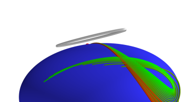
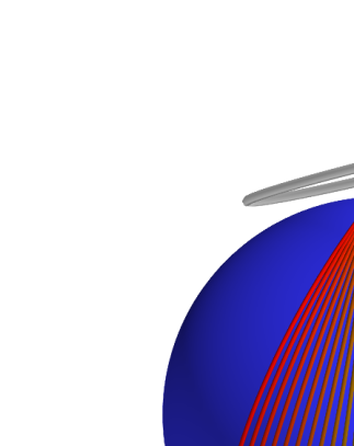
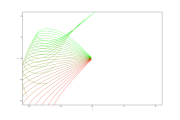
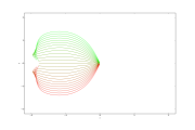
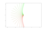
Figure 4: Curves satisfying the MPP equations (top row) and corresponding anti-development (bottom row) on three surfaces embedded in $\mathbb{R}^{3}$: An ellipsoid (left), a sphere (middle), a hyperbolic surface (right). The family of curves is generated by rotating by $\pi/2$ radians the anisotropic covariance represented in the initial frame $u_{0}$ and displayed in the gray ellipse.

The geodesic system is again given by the Hamilton-Jacobi equations. As in the full-rank case, the system is specified by the derivatives of $g_{F^{k}M}$:

$$\partial_{y^{l}}g_{F^{k}M}^{ij}=W\indices{{}^{ij}_{,l}}\ ,\quad\partial_{y^{l}}g_{F^{k}M}^{ij_{\beta}}=-W\indices{{}^{ih}_{,l}}\Gamma^{j_{\beta}}_{h}-W^{ih}\Gamma^{j_{\beta}}_{h,l}\ ,\quad\partial_{y^{l}}g_{F^{k}M}^{i_{\alpha}j}=-\Gamma^{i_{\alpha}}_{h,l}W^{hj}-\Gamma^{i_{\alpha}}_{h}W\indices{{}^{hj}_{,l}}\ ,$$

$$\partial_{y^{l}}g_{F^{k}M}^{i_{\alpha}j_{\beta}}=\Gamma^{i_{\alpha}}_{k,l}W^{kh}\Gamma^{j_{\beta}}_{h}+\Gamma^{i_{\alpha}}_{k}W\indices{{}^{kh}_{,l}}\Gamma^{j_{\beta}}_{h}+\Gamma^{i_{\alpha}}_{k}W^{kh}\Gamma^{j_{\beta}}_{h,l}\ ,$$

$$\partial_{y^{l_{\zeta}}}g_{F^{k}M}^{ij}=W\indices{{}^{ij}_{,l_{\zeta}}}\ ,\quad\partial_{y^{l_{\zeta}}}g_{F^{k}M}^{ij_{\beta}}=-W\indices{{}^{ih}_{,l_{\zeta}}}\Gamma^{j_{\beta}}_{h}-W^{ih}\Gamma^{j_{\beta}}_{h,l_{\zeta}}\ ,\quad\partial_{y^{l_{\zeta}}}g_{F^{k}M}^{i_{\alpha}j}=-\Gamma^{i_{\alpha}}_{h}W\indices{{}^{hj}_{,l_{\zeta}}}-\Gamma^{i_{\alpha}}_{h,l_{\zeta}}W^{hj}\ ,$$

$$\partial_{y^{l_{\zeta}}}g_{F^{k}M}^{i_{\alpha}j_{\beta}}=\Gamma^{i_{\alpha}}_{k,l_{\zeta}}W^{kh}\Gamma^{j_{\beta}}_{h}+\Gamma^{i_{\alpha}}_{k}W\indices{{}^{kh}_{,l_{\zeta}}}\Gamma^{j_{\beta}}_{h}+\Gamma^{i_{\alpha}}_{k}W^{kh}\Gamma^{j_{\beta}}_{h,l_{\zeta}}\ ,$$

$$\Gamma^{i_{\alpha}}_{h,l_{\zeta}}=\partial_{y^{l_{\zeta}}}\left(\Gamma\indices{{}^{i}_{hk}}u^{k}_{\alpha}\right)=\delta^{\zeta\alpha}\Gamma\indices{{}^{i}_{hl}}\ ,\quad W\indices{{}^{ij}_{,l}}=\lambda g\indices{{}_{R}^{ij}{}_{,l}}\ ,\quad W\indices{{}^{ij}_{,l_{\zeta}}}=\delta^{il}u^{j}_{\zeta}+\delta^{jl}u^{i}_{\zeta}\ .$$

Note that the introduction of the Riemannian metric $g_{R}$ implies that $W^{ij}$ are now dependent on the manifold coordinates $x^{i}$.

6 Numerical Experiments

We aim at visualizing most probable paths for the driving process and projections of curves satisfying the MPP equations (13) in two cases: On 2D surfaces embedded in $\mathbb{R}^{3}$ and on finite dimensional landmark manifolds that arise from equipping a subset of the diffeomorphism group with a right-invariant metric and letting the action descend to the landmarks by a left action. The surface examples are implemented in Python using the Theano [TARA⁺16] framework for symbolic operations, automatic differentiation, and numerical evaluation. The landmark equations are detailed below and implemented in Numpy using Numpy’s standard ODE integrators. The code for running the experiments is available at http://bitbucket.com/stefansommer/mpps/.

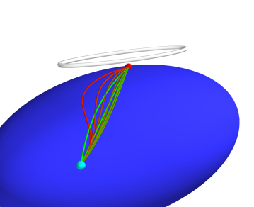
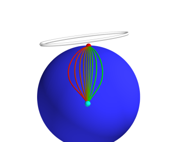
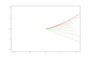
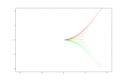
Figure 5: Minimizing normal MPPs between two fixed points (red/cyan). From isotropic covariance (top row, left) to anisotropic (top row, right) on $\mathbb{S}^{2}$. Compare with minimizing Riemannian geodesic (black curve). The MPP travels longer in the directions of high variance. Families of curves (middle row) and corresponding anti-development (bottom row) on the three surfaces in Figure 4. The family of curves is generated by rotating the covariance matrix as in Figure 4. Notice how the varying anisotropy affects the resulting minimizing curves, and how the anti-developed curves end at different points in $\mathbb{R}^{2}$.

6.1 Embedded Surfaces

We visualize normal MPPs and projections of curves satisfying the MPP equations (13) on surfaces embedded in $\mathbb{R}^{3}$ in three cases: The sphere $\mathbb{S}^{2}$, on an ellipsoid, and on a hyperbolic surface. The surfaces are chosen in order to have both positive and negative curvature, and to have varying degree of symmetry. In all cases, an open subset of the surfaces are represented in a single chart by a map $F:\mathbb{R}^{2}\rightarrow\mathbb{R}^{3}$. For the sphere and ellipsoid, this gives a representation of the surface except for the south pole. The metric and Christoffel symbols are calculated using the symbolic differentiation features of Theano. The integration are performed by a simple Euler integrator.

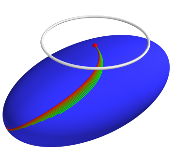
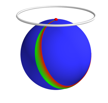
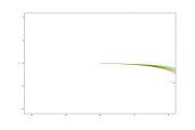
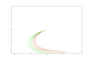
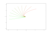
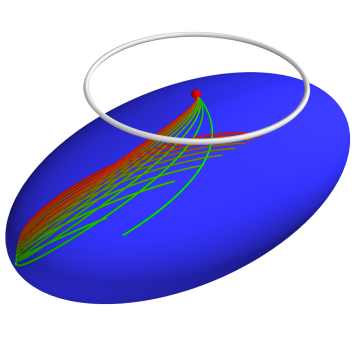
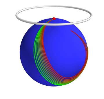
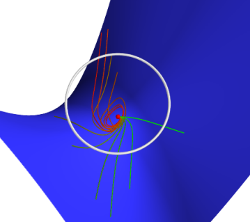
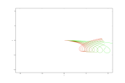
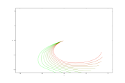
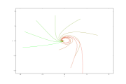
Figure 6: With the setup of Figure 4,5, generated families of curves by varying the vertical $V^{*}FM$ part of the initial momentum $\xi_{0}\in T^{*}FM$ but keeping the base point and frame $u_{0}$ fixed. The vertical part allows varying degree of “twisting” of the curve.

Figures 4-6 shows families of curves satisfying the MPP equations in three cases: (1) With fixed starting point $x_{0}\in M$ and initial velocity $\dot{x}_{0}\in TM$ but varying anisotropy represented by changing frame $u$ in the fiber above $x_{0}$; (2) minimizing normal MPPs with fixed starting point and endpoint $x_{0},x_{1}\in M$ but changing frame $u$ above $x_{0}$; (3) fixed starting point $x_{0}\in M$ and frame $u$ but varying $V^{*}FM$ vertical part of the initial momentum $\xi_{0}\in T^{*}FM$. The first and second cases thus shows the effect of varying anisotropy while the third case illustrates the effect of the “twist” the $d^{2}$ degrees in the vertical momentum allows. Note the displayed anti-developed curves in $\mathbb{R}^{2}$ that for classical ${\mathcal{C}}$ geodesics would always be straight lines.

6.2 LDDMM Landmark Equations

We here give a example of the MPP equations using the finite dimensional landmark manifolds that arise from right invariant metrics on subsets of the diffeomorphism group in the Large Deformation Diffeomorphic Metric Mapping (LDDMM) framework [You10]. The LDDMM metric can be conveniently expressed as a cometric, and, using a rank-deficient inner product $g_{F^{k}M}$ as discussed in Section 5, we can obtain a reduction of the system of equations to $2(2N+2Nk)$ compared to $2(2N+(2N)^{2})$ with $N$ landmarks in $\mathbb{R}^{2}$.

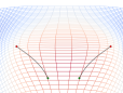
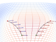
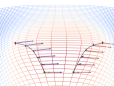
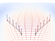
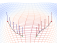
(a)                       (b)                       (c)                       (d)                       (e)

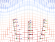
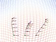
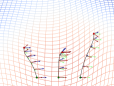
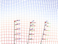
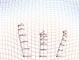
Figure 7: (top row) Matching of two landmarks (green) to two landmarks (red) by (a) computing a minimizing Riemannian geodesic on the landmark manifold, and (b-e) minimizing MPPs with added covariance (arrows) in $\mathbb{R}^{2}$ horizontal direction (b-c) and vertical (d-e). The action of the corresponding diffeomorphisms on a regular grid is visualized by the deformed grid which is colored by the warp strain. The added covariance allows the paths to have more movement in the horizontal and vertical direction respectively because the anisotropically weighted metric penalizes high-covariance directions less. (bottom row) Five landmark trajectories with fixed initial velocity and anisotropic covariance but varying $V^{*}FM$ vertical initial momentum $\xi_{0}$. Changing the vertical momentum “twists” the paths.

Let $\{p_{1},\ldots,p_{N}\}$ be landmarks in a subset $\Omega\subset\mathbb{R}^{d}$. The diffeomorphism group $\mathrm{Diff}(\Omega)$ acts on the left on landmarks with the action $\varphi.\{p_{1},\ldots,p_{N}\}=\{\varphi(p_{1}),\ldots,\varphi(p_{N})\}$. In LDDMM, a Hilbert space structure is imposed on a linear subspace $V$ of $L^{2}(\Omega,\mathbb{R}^{d})$ using a self-adjoint operator $L:V\rightarrow V^{*}\subset L^{2}(\Omega,\mathbb{R}^{d})$ and defining the inner product $\left<\cdot,\cdot\right>_{V}$ by

$$\left<v,w\right>_{V}=\left<Lv,w\right>_{L^{2}}\ .$$

Under sufficient conditions on $L$, $V$ is reproducing and admits a kernel $K$ inverse to $L$. $K$ is a Green’s kernel when $L$ is a differential operator, or $K$ can be a Gaussian kernel. The Hilbert structure on $V$ gives a Riemannian metric on a subset $G_{V}\subset\mathrm{Diff}(\Omega)$ by setting $\|v\|_{\varphi}^{2}=\|v\circ\varphi^{-1}\|_{V}^{2}$, i.e. regarding $\left<\cdot,\cdot\right>_{V}$ an inner product on $T_{\mathrm{Id}}G_{V}$ and extending the metric to $G_{V}$ by right-invariance. This Riemannian metric descends to a Riemannian metric on the landmark space.

Let $M$ be the manifold $M=\{(p_{1}^{1},\ldots,p_{1}^{d},\ldots,p_{N}^{1},\ldots,p_{N}^{d})|(p_{i}^{1},\ldots,p_{i}^{d})\in\mathbb{R}^{d}\}$. The LDDMM metric on the landmark manifold $M$ is directly related to the kernel $K$ when written as a cometric $g_{p}(\xi,\eta)=\sum_{i,j=1}^{N}\xi^{i}K(p_{i},p_{j})\eta^{j}$. Letting $i^{k}$ denote the index of the $k$th component of the $i$th landmark, the cometric is in coordinates $g_{p}^{i^{k}j^{l}}=K(p_{i},p_{j})_{k}^{l}$. The Christoffel symbols can be written in terms of derivatives of the cometric $g^{ij}$ [Mic08] (recall that $\delta^{i}_{j}=g^{ik}g_{kj}=g_{jk}g^{ki}$)

$$\Gamma\indices{{}^{k}_{ij}}=\frac{1}{2}g_{ir}\left(g^{kl}g\indices{{}^{rs}_{,l}}-g^{sl}g\indices{{}^{rk}_{,l}}-g^{rl}g\indices{{}^{ks}_{,l}}\right)g_{sj}\ .$$ (18)

This relation comes from the fact that $g_{jm,k}=-g_{jr}g\indices{{}^{rs}_{,k}}g_{sm}$ gives the derivative of the metric. The derivatives of the cometric is simply $g\indices{{}^{i^{k}j^{l}}_{,r^{q}}}=(\delta_{r}^{i}+\delta_{r}^{j})\partial_{p_{r}^{q}}K(p_{i},p_{j})_{k}^{l}$. Using (18), derivatives of the Christoffel symbols can be computed

$$\Gamma\indices{{}^{k}_{ij}{}_{,\xi}} =\frac{1}{2}g_{ir,\xi}\left(g^{kl}g\indices{{}^{rs}_{,l}}-g^{sl}g\indices{{}^{rk}_{,l}}-g^{rl}g\indices{{}^{ks}_{,l}}\right)g_{sj}+\frac{1}{2}g_{ir}\left(g^{kl}g\indices{{}^{rs}_{,l}}-g^{sl}g\indices{{}^{rk}_{,l}}-g^{rl}g\indices{{}^{ks}_{,l}}\right)g_{sj,\xi}$$

$$\qquad+\frac{1}{2}g_{ir}\left(g\indices{{}^{kl}_{,\xi}}g\indices{{}^{rs}_{,l}}+g^{kl}g\indices{{}^{rs}_{,l\xi}}-g\indices{{}^{sl}_{,\xi}}g\indices{{}^{rk}_{,l}}-g^{sl}g\indices{{}^{rk}_{,l\xi}}-g\indices{{}^{rl}_{,\xi}}g\indices{{}^{ks}_{,l}}-g^{rl}g\indices{{}^{ks}_{,l\xi}}\right)g_{sj}\ .$$

This provides the full data for numerical integration of the evolution equations on $F^{k}M$.

In Figure 7 top row, we plot minimizing normal MPPs on the landmark manifold with two landmarks and varying covariance in the $\mathbb{R}^{2}$ horizontal and vertical direction. The plot shows the landmark equivalent of experiment in Figure 5. Note how adding covariance in the horizontal and vertical direction respectively allows the minimizing normal MPP to varying more in these directions because the anisotropically weighted metric penalizes high-covariance directions less.

Figure 7 bottom row shows five curves satisfying the MPP equations with varying vertical $V^{*}FM$ initial momentum similarly to the plots in Figure 6. Again, we see how the extra degrees of freedom allows the paths to twist generating a higher-dimensional family than classical geodesics with respect to ${\mathcal{C}}$.

7 Discussion and Concluding Remarks

Incorporating anisotropy in models for data in non-linear spaces via the frame bundle as pursued in this paper leads to a sub-Riemannian structure and metric. A direct implication is that most probable paths to observed data in the sense of sequences of stochastic steps of a driving semi-martingale are not related to geodesics in the classical sense. Instead, a best estimate of the sequence of steps $w_{t}\in\mathbb{R}^{d}$ that leads to an observation $x=\varphi_{u}(w_{t})|_{t=1}$ is an MPP in the sense of Definition 1. As shown in the paper, these paths are generally not geodesics or polynomials with respect to the connection on the manifold. In particular, if $M$ has a Riemannian structure, the MPPs are generally neither Riemannian geodesics or Riemannian polynomials. Below, we discuss statistical implications of this result.

7.1 Statistical Estimators

Metric distances and Riemannian geodesics have been the traditional vehicle for representing observed data in non-linear spaces. Most fundamentally, the sample Frechét mean

$$\hat{x}=\textrm{argmin}_{x\in M}\sum_{i=1}^{N}d_{g_{R}}\left(x,x_{i}\right)^{2}$$ (19)

of observed data $x_{1},\ldots,x_{N}\in M$ relies crucially on the Riemannian distance $d_{g_{R}}$ connected to the metric $g_{R}$. Many PCA constructs, e.g. Principal Geodesics Analysis [FLPJ04], uses the Riemannian $\mathrm{Exp}$ and $\mathrm{Log}$ maps to map between linear tangent spaces and the manifold. These maps are defined from the Riemannian metric and Riemannian geodesics. Distributions modelled as in the random orbit model [MBC⁺97] or Bayesian models [ZF13, ZSF13] again rely on geodesics with random initial conditions.

Using the frame bundle sub-Riemannian metric $g_{FM}$, we can define an estimator analogous to the Riemannian Frechét mean estimator. Assuming the covariance is a priori known, the estimator

$$\hat{x}=\textrm{argmin}_{u\in s(M)}\sum_{i=1}^{N}d_{FM}\left(u,\pi^{-1}(x_{i})\right)^{2}$$ (20)

acts correspondingly to the Frechét mean estimator (19). Here $s\in\Gamma(FM)$ is a (local) section of $FM$ that to $x\in M$ connects the known covariance represented by $s(x)\in FM$. The distances $d_{FM}\left(u,\pi^{-1}(x_{i})\right)$, $u=s(x)$ are realized by MPPs from the mean candidate $x$ to the fibers $\pi^{-1}(x_{i})$. The Frechét mean problem is thus lifted to the frame bundle with the anisotropic weighting incorporated in the metric $g_{FM}$. This metric is not related to $g_{R}$ except for its dependence on the connection $\mathcal{C}$ that can be defined as the Levi-Civita connection of $g_{R}$. The fundamental role of the distance $d_{g_{R}}$ and $g_{R}$ geodesics in (19) is thus removed.

Because covariance is an integral part of the model, sample covariance can also be estimated directly along with the sample mean. In [SS16], the estimator

$$\hat{u}=\textrm{argmin}_{u\in FM}\sum_{i=1}^{N}d_{FM}\left(u,\pi^{-1}(x_{i})\right)^{2}-N\log(\mathrm{det}_{g_{R}}u)$$ (21)

is suggested. The normalizing term $-N\log(\mathrm{det}_{g_{R}}u)$ is derived such that the estimator exactly corresponds to the maximum likelihood estimator of mean and covariance for Euclidean Gaussian distributions. The determinant is defined via $g_{R}$, and the term acts to prevent the covariance from approaching infinity. Maximum likelihood estimators of mean and covariance for normally distributed Euclidean data have unique solutions in the sample mean and sample covariance matrix, respectively. Uniqueness of the Frechét mean (19) is only ensured for sufficiently concentrated data. For the estimator (21), existence and uniqueness properties are not immediate, and more work is needed in order to find necessary and sufficient conditions.

7.2 Priors and Low-Rank Estimation

The low-rank cometric formulation pursued in Section 5 gives a natural restriction of (21) to $u\in F^{k}M$, $1\leq k\leq d$. As for Euclidean PCA, most variance is often captured in the span of the first $k$ eigenvectors with $k\ll d$. Estimates of the remaining eigenvectors are generally ignored as the variance of the eigenvector estimates increases as the noise captured in the span of the last eigenvectors becomes increasingly uniform. The low-rank cometric restricts the estimation to only the first $k$ eigenvectors and thus builds the construction directly into the model. In addition, it makes numerical implementation feasible because a numerical representation need only store and evolve $d\times k$ matrices. As a different approach for regularizing the estimator (21), the normalizing term $-N\log(\mathrm{det}_{g_{R}}u)$ can be extended with other priors, e.g. an $L^{1}$-type penalizing term. Such priors can potentially partly remove existence and uniqueness issues and result in additional sparsity properties that can benefit numerical implementations. The effects of such priors has yet to be investigated.

In the $k=d$ case, the number of degrees of freedoms for the MPPs grows quadratically in the dimension $d$. This naturally increases the variance of any MPP estimate given only one sample from its trajectory. The low-rank cometric formulation reduces the growth to linear in $d$. The number of degrees of freedom is however still $k$ times larger than for Riemannian geodesics. With longitudinal data, more samples per trajectory can be obtained reducing the variance and allowing a better estimate of the MPP. However, for the estimators (20) and (21) above, estimates of the actual optimal MPPs are not needed, only their squared length. It can be hypothesized that the variance of the length estimates is lower than the variance of the estimates of the corresponding MPPs. Further investigation regarding this will be the subject of future work.

7.3 Conclusion

The underlying model of anisotropy used in this paper originates from the anisotropic normal distributions formulated in [Som15] and the diffusion PCA framework [Som14]. Because many statistical models are defined using normal distributions, this approach for incorporating anisotropy extends to models such as linear regression. We expect that finding most probable paths in other statistical models such as regressions models can be carried out with a program similar to the program presented in this paper.

The difference between MPPs and geodesics shows that the geometric and metric properties of geodesics, zero acceleration and local distance minimization, are not directly related to statistical properties such as maximizing path probability. Whereas the concrete application and model determines if metric or statistical properties are fundamental, most statistical models are formulated without referring to metric properties of the underlying space. It can therefore be argued that the direct incorporation of anisotropy and the resulting MPPs are natural in the context of many models of data variation in non-liner spaces.

References

• [AD99] Lars Andersson and Bruce K Driver, Finite Dimensional Approximations to Wiener Measure and Path Integral Formulas on Manifolds, Journal of Functional Analysis 165 (1999), no. 2, 430–498.
• [Blo03] A. M. Bloch, Nonholonomic Mechanics and Control, Interdisciplinary Applied Mathematics, vol. 24, Springer New York, New York, NY, 2003.
• [CSLC01] M. Camarinha, F. Silva Leite, and P. Crouch, On the geometry of Riemannian cubic polynomials, Differential Geometry and its Applications 15 (2001), no. 2, 107–135.
• [Elw88] David Elworthy, Geometric aspects of diffusions on manifolds, École d’Été de Probabilités de Saint-Flour XV–XVII, 1985–87 (Paul-Louis Hennequin, ed.), Lecture Notes in Mathematics, no. 1362, Springer Berlin Heidelberg, 1988, pp. 277–425 (en).
• [FK82] Takahiko Fujita and Shin-ichi Kotani, The Onsager-Machlup function for diffusion processes, Journal of Mathematics of Kyoto University 22 (1982), no. 1, 115–130 (EN). MR MR648558
• [FLPJ04] P.T. Fletcher, Conglin Lu, S.M. Pizer, and Sarang Joshi, Principal geodesic analysis for the study of nonlinear statistics of shape, Medical Imaging, IEEE Transactions on (2004).
• [Fr48] M. Frechet, Les elements aleatoires de nature quelconque dans un espace distancie, Ann. Inst. H. Poincare 10 (1948), 215–310.
• [HFJ14] Jacob Hinkle, P. Thomas Fletcher, and Sarang Joshi, Intrinsic Polynomials for Regression on Riemannian Manifolds, Journal of Mathematical Imaging and Vision 50 (2014), no. 1-2, 32–52 (en).
• [HHM10] Stephan Huckemann, Thomas Hotz, and Axel Munk, Intrinsic shape analysis: Geodesic PCA for Riemannian manifolds modulo isometric Lie group actions, Statistica Sinica 20 (2010), no. 1, 1–100.
• [Hsu02] Elton P. Hsu, Stochastic Analysis on Manifolds, American Mathematical Soc., 2002 (en).
• [JDM12] Sungkyu Jung, Ian L. Dryden, and J. S. Marron, Analysis of principal nested spheres, Biometrika 99 (2012), no. 3, 551–568 (en).
• [Kar77] H. Karcher, Riemannian center of mass and mollifier smoothing, Communications on Pure and Applied Mathematics 30 (1977), no. 5, 509–541.
• [KSM93] Ivan Kolář, Jan Slovák, and Peter W. Michor, Natural Operations in Differential Geometry, Springer Berlin Heidelberg, Berlin, Heidelberg, 1993 (en).
• [LK08] Fátima Silva Leite and Krzysztof Andrzej Krakowski, Covariant differentiation under rolling maps (eng).
• [MBC+97] M. Miller, A. Banerjee, G. Christensen, S. Joshi, N. Khaneja, U. Grenander, and L. Matejic, Statistical methods in computational anatomy, Statistical Methods in Medical Research 6 (1997), no. 3, 267–299 (eng).
• [Mic08] Mario Micheli, The differential geometry of landmark shape manifolds: metrics, geodesics, and curvature, Ph.D. thesis, Brown University, Providence, USA, 2008.
• [Mok78] Kam-Ping Mok, On the differential geometry of frame bundles of Riemannian manifolds, Journal Fur Die Reine Und Angewandte Mathematik 1978 (1978), no. 302, 16–31.
• [MR99] Jerrold E. Marsden and Tudor S. Ratiu, Introduction to Mechanics and Symmetry, Texts in Applied Mathematics, vol. 17, Springer New York, New York, NY, 1999.
• [NHP89] Lyle Noakes, Greg Heinzinger, and Brad Paden, Cubic splines on curved spaces, IMA Journal of Mathematical Control and Information 6 (1989), no. 4, 465–473.
• [Pen06] Xavier Pennec, Intrinsic Statistics on Riemannian Manifolds: Basic Tools for Geometric Measurements, J. Math. Imaging Vis. 25 (2006), no. 1, 127–154.
• [Pen15]  , Barycentric Subspaces and Affine Spans in Manifolds, Geometric Science of Information (Frank Nielsen and Frédéric Barbaresco, eds.), Lecture Notes in Computer Science, Springer International Publishing, October 2015, DOI: 10.1007/978-3-319-25040-3_2, pp. 12–21 (en).
• [Som13] Stefan Sommer, Horizontal Dimensionality Reduction and Iterated Frame Bundle Development, Geometric Science of Information, LNCS, Springer, 2013, pp. 76–83.
• [Som14]  , Diffusion Processes and PCA on Manifolds, Mathematisches Forschungsinstitut Oberwolfach https://www.mfo.de/document/1440a/OWR_2014\_44.pdf, 2014.
• [Som15]  , Anisotropic Distributions on Manifolds: Template Estimation and Most Probable Paths, Information Processing in Medical Imaging, Lecture Notes in Computer Science, vol. 9123, Springer Berlin Heidelberg, 2015, pp. 193–204.
• [SS16] Stefan Sommer and Anne Marie Svane, Modelling Anisotropic Covariance using Stochastic Development and Sub-Riemannian Frame Bundle Geometry, Journal of Geometric Mechanics (2016), in press, arXiv:1512.08544 [math, stat]
• [Str86] Robert S. Strichartz, Sub-Riemannian geometry, Journal of Differential Geometry 24 (1986), no. 2, 221–263 (EN). MR MR862049
• [TARA+16] The Theano Development Team, Rami Al-Rfou, Guillaume Alain, Amjad Almahairi, Christof Angermueller, Dzmitry Bahdanau, Nicolas Ballas, Frédéric Bastien, Justin Bayer, Anatoly Belikov, Alexander Belopolsky, Yoshua Bengio, Arnaud Bergeron, James Bergstra, Valentin Bisson, Josh Bleecher Snyder, Nicolas Bouchard, Nicolas Boulanger-Lewandowski, Xavier Bouthillier, Alexandre de Brébisson, Olivier Breuleux, Pierre-Luc Carrier, Kyunghyun Cho, Jan Chorowski, Paul Christiano, Tim Cooijmans, Marc-Alexandre Côté, Myriam Côté, Aaron Courville, Yann N. Dauphin, Olivier Delalleau, Julien Demouth, Guillaume Desjardins, Sander Dieleman, Laurent Dinh, Mélanie Ducoffe, Vincent Dumoulin, Samira Ebrahimi Kahou, Dumitru Erhan, Ziye Fan, Orhan Firat, Mathieu Germain, Xavier Glorot, Ian Goodfellow, Matt Graham, Caglar Gulcehre, Philippe Hamel, Iban Harlouchet, Jean-Philippe Heng, Balázs Hidasi, Sina Honari, Arjun Jain, Sébastien Jean, Kai Jia, Mikhail Korobov, Vivek Kulkarni, Alex Lamb, Pascal Lamblin, Eric Larsen, César Laurent, Sean Lee, Simon Lefrancois, Simon Lemieux, Nicholas Léonard, Zhouhan Lin, Jesse A. Livezey, Cory Lorenz, Jeremiah Lowin, Qianli Ma, Pierre-Antoine Manzagol, Olivier Mastropietro, Robert T. McGibbon, Roland Memisevic, Bart van Merriënboer, Vincent Michalski, Mehdi Mirza, Alberto Orlandi, Christopher Pal, Razvan Pascanu, Mohammad Pezeshki, Colin Raffel, Daniel Renshaw, Matthew Rocklin, Adriana Romero, Markus Roth, Peter Sadowski, John Salvatier, François Savard, Jan Schlüter, John Schulman, Gabriel Schwartz, Iulian Vlad Serban, Dmitriy Serdyuk, Samira Shabanian, Etienne Simon, Sigurd Spieckermann, S. Ramana Subramanyam, Jakub Sygnowski, Jérémie Tanguay, Gijs van Tulder, Joseph Turian, Sebastian Urban, Pascal Vincent, Francesco Visin, Harm de Vries, David Warde-Farley, Dustin J. Webb, Matthew Willson, Kelvin Xu, Lijun Xue, Li Yao, Saizheng Zhang, and Ying Zhang, Theano: A Python framework for fast computation of mathematical expressions, arXiv:1605.02688 [cs] (2016), arXiv: 1605.02688.
• [Tau11] Clifford Henry Taubes, Differential Geometry: Bundles, Connections, Metrics and Curvature, 1 edition ed., Oxford University Press, Oxford ; New York, December 2011 (English).
• [TB99] Michael E. Tipping and Christopher M. Bishop, Probabilistic Principal Component Analysis, Journal of the Royal Statistical Society. Series B 61 (1999), no. 3, 611–622.
• [VMYT04] M. Vaillant, M.I. Miller, L. Younes, and A. Trouvé, Statistics on diffeomorphisms via tangent space representations, NeuroImage 23 (2004), no. Supplement 1, S161–S169.
• [You10] Laurent Younes, Shapes and Diffeomorphisms, Springer, 2010.
• [ZF13] Miaomiao Zhang and P.T. Fletcher, Probabilistic Principal Geodesic Analysis, NIPS, 2013, pp. 1178–1186.
• [ZSF13] Miaomiao Zhang, Nikhil Singh, and P. Thomas Fletcher, Bayesian Estimation of Regularization and Atlas Building in Diffeomorphic Image Registration, Information Processing for Medical Imaging (IPMI), Lecture Notes in Computer Science, Springer, 2013, pp. 37–48 (en).