Detailed Hi kinematics of Tully-Fisher calibrator galaxies

Abstract

We present spatially–resolved Hi kinematics of 32 spiral galaxies which have Cepheid or/and Tip of the Red Giant Branch distances, and define a calibrator sample for the Tully-Fisher relation. The interferometric Hi data for this sample were collected from available archives and supplemented with new GMRT observations. This paper describes an uniform analysis of the Hi kinematics of this inhomogeneous data set. Our main result is an atlas for our calibrator sample that presents global Hi profiles, integrated Hi column–density maps, Hi surface density profiles and, most importantly, detailed kinematic information in the form of high–quality rotation curves derived from highly–resolved, two–dimensional velocity fields and position–velocity diagrams.

1 Introduction

The Tully-Fisher relation (TFr) is one of the main scaling relations for rotationally supported galaxies, describing an empirical correlation between the luminosity or visible mass of a spiral galaxy and its rotational velocity or dynamical mass (Tully & Fisher, 1977). Numerous observational studies of the statistical properties of the TFr have been undertaken in the past. Generally, their aim was to find observables that reduce the scatter in the relation, and thus improve the distance measure to spiral galaxies. An accurate distance measure is necessary to address some of the main cosmological questions pertaining to the local Universe, such as the value of the Hubble constant, the local large–scale structure and the local cosmic flow field, e.g. Tully & Courtois 2012, hereafter TC12.

Use of the implied scaling law and understanding its origin is one of the main challenges for theories of galaxy formation and evolution. In particular the detailed statistical properties of the TFr provide important constraints to semi–analytical models and numerical simulations of galaxy formation and evolution. It is an important test for theoretical studies to reproduce the slope, scatter and the zero point of the TFr in different photometric bands simultaneously. Recent cosmological simulations of galaxy formation have reached sufficient maturity to construct sufficiently realistic galaxies that follow the observed TFr (Marinacci et al., 2014; Vogelsberger et al., 2014; Schaye et al., 2015).

An important outstanding issue, however, is how to connect the results from simulations to the multitude of observational studies, which often do not agree with each other (McGaugh, 2012; Zaritsky et al., 2014). Moreover, while performing these comparison tests, it is important to ensure that the galaxy parameters derived from simulations and observations have the same physical meaning. For example, for simulated galaxies the circular velocity of a galaxy is usually derived from the potential of the dark matter halo, while the observed velocity, based on the width of the global Hi profile obtained with single–dish telescopes, is a good representation for the dark matter halo potential only in rather limited cases. Note that the rotational velocity of a galaxy, inferred from the width of its global Hi profile, can be directly related to the dark matter potential only when the gas is in co–planar, circular orbits and the rotation curve has reached the turnover to a constant velocity at radii properly sampled by the gas disk. However, this is often not the case as galaxies display a variety of rotation curves shapes, which can not be characterised with a single parameter such as the corrected width of the global Hi line profile. Furthermore, the number of observational studies that take into account the two–dimensional distribution of Hi and the detailed geometry and kinematics of a galaxy’s disk is rather limited.

With the developments of new methods and instruments, the observed scatter in the Tully-Fisher relation has decreased significantly, mainly due to more accurate photometric measurements. Photographic magnitudes (Tully & Fisher, 1977) were improved upon by CCD photometry. The advent of infra–red arrays shifted photometry to the JHK bands, minimizing extinction corrections, and then to space–based infra–red photometry with the Spitzer Space Telescope (Werner et al., 2004), which better samples the older stellar population and maximizes photometric calibration stability. As was shown by Sorce et al. (2012), the measurement errors on the total $3.6\mu m$ luminosity are reduced to a point where they no longer contribute significantly to the observed scatter in the Tully–Fisher relation. Hence, other measurement errors, such as uncertainties on a galaxy’s inclination and/or rotational velocity, combined with a certain intrinsic scatter are responsible for the total observed scatter.

Figure 1: The distribution of morphological types of our sample galaxies.

It was shown by Verheijen (2001), with a study of nearly equidistant spiral galaxies in the Ursa Major cluster with deep K’–band photometry, that the observed scatter in the Tully–Fisher relation can be reduced significantly when the measured velocity of the outer, flat part of the Hi rotation curve (V_flat) is used instead of the rotational velocity as estimated from the width of the global Hi profile. Indeed, the spatially-resolved, two–dimensional velocity fields of gas disks, obtained with radio interferometric arrays, often reveal the presence of warps, streaming motions and kinematic lopsidedness of the gas disks, while the global Hi profiles do not allow the identification of such features. Therefore, the width of a global Hi line profile, albeit easily obtained with a single–dish telescope, may not be an accurate representation of V_flat. Moreover, the analysis of spatially resolved Hi kinematics shows that the rotation curves of spiral galaxies are not always flat and featureless. Rotation curves may still be rising at the outermost observable edge of the gas disk, in which case the width of the global Hi profile provides a lower limit on V_flat. Rotation curves may also be declining beyond an initial turnover radius, in which case V_flat derived from the rotation curve is systematically lower than the circular velocity derived from the corrected width of the global Hi profile. In this paper, we investigate the differences between three measures of the rotational velocity of spiral galaxies: The rotational velocity from the corrected width of the global Hi profile, the maximal rotation velocity of the rotation curve (V_max) and the rotational velocity of the outer flat part of the rotation curve (V_flat). The effects of these different velocity measures on the observed scatter and the intrinsic properties of the TFr will be discussed in a forthcoming paper.

To derive V_max and V_flat we analyse in detail the Hi synthesis imaging data for a Tully-Fisher calibrator sample of 32 nearby, well–resolved galaxies and present these data in the form of an Atlas and tables. We will discuss the identification and corrections made for warps and streaming motions in the gas disks when deriving the Hi rotation curves. Forthcoming papers will use these data to investigate the luminosity–based TFr using panchromatic photometric data, as well as the baryonic TFr for the same calibrator sample.

This paper is organised as follows: Section 2 describes the sample of selected galaxies. Section 3 presents the data collection and analysis, including subsections on the comparison between the rotational velocities obtained from the rotation curves and the corrected width of the global Hi profiles. Section 4 presents the properties of the gaseous disks of the sample galaxies. A summary and concluding remarks are presented in Section 5. The Atlas is described in the Appendix, together with notes on individual galaxies.

Name	Hubble type	P.A.	Incl.	Log$\,d_{25}$	$m_{T}^{b,i}[3.6]$	$\mu_{0}^{i}[3.6]$	Log$\,h_{r}[3.6]$	Distance
		deg	deg	arcsec	mag	mag arcsec-2	arcsec	Mpc
NGC 0055	SBm	101	86	2.47	5.64	17.54	2.32	2.09
NGC 0224	SAb	35	78	3.25	0.48	17.74	2.46	0.76
NGC 0247	SABd	166	76	2.29	6.27	18.52	2.26	3.45
NGC 0253	SABc	52	81	2.42	3.37	14.36	2.10	3.45
NGC 0300	SAd	114	46	2.29	5.56	25.30	2.18	1.93
NGC 0925	SABd	104	57	2.03	7.24	20.73	1.95	9.16
NGC 1365	SBb	20	54	2.08	5.91	27.71	1.85	17.94
NGC 2366	IBm	32	74	1.64	9.76	21.20	2.07	3.31
NGC 2403	SABc	126	60	2.30	5.52	19.51	2.47	3.19
NGC 2541	SAc	169	63	1.48	9.16	20.22	1.60	11.22
NGC 2841	SAb	148	66	1.84	5.70	16.90	1.79	14.01
NGC 2976	SAc	143	60	1.86	6.95	19.15	1.78	3.56
NGC 3031	SAb	157	59	2.33	3.40	18.68	2.15	3.59
NGC 3109	SBm	93	90	2.20	7.76	18.25	2.08	1.30
NGC 3198	SBc	32	70	1.81	7.44	17.37	1.61	13.80
IC 2574	SABm	50	69	2.11	8.60	22.18	2.04	3.81
NGC 3319	SBc	34	59	1.56	9.05	22.80	1.74	13.30
NGC 3351	SBb	10	47	1.86	6.45	24.77	1.68	10.91
NGC 3370	SAc	143	58	1.38	8.70	20.43	1.23	0.23
NGC 3621	SAd	161	66	1.99	6.37	17.57	1.71	7.01
NGC 3627	SABb	173	60	2.01	5.39	19.01	1.78	10.04
NGC 4244	SAc	42	90	2.21	7.39	18.34	2.47	4.20
NGC 4258	SABb	150	69	2.26	4.95	18.89	2.24	7.31
NGC 4414	SAc	166	55	1.29	6.56	23.03	1.69	17.70
NGC 4535	SABc	180	45	1.91	6.80	25.28	1.62	15.77
NGC 4536	SABc	118	71	1.85	7.17	18.03	1.70	15.06
NGC 4605	SBc	125	69	1.77	7.22	18.29	1.66	5.32
NGC 4639	SABb	130	55	1.46	8.28	26.64	1.27	21.87
NGC 4725	SABa	36	58	1.99	5.93	21.91	1.79	12.76
NGC 5584	SAB	157	44	1.50	8.87	25.27	1.39	22.69
NGC 7331	SAb	169	66	1.96	5.45	19.12	1.79	14.72
NGC 7793	SAd	83	53	2.02	6.43	22.30	1.85	3.94

Table 1: The Tully-Fisher Calibrator Sample. Column (1): galaxy name (as shown in NED); Column (2): Hubble type (as shown in NED); Column (3): optical position angle of the disk from TC12; Column (4): optical inclination of the disk from TC12; Column (5): optical diameter (as shown in NED); Column (6): total apparent magnitude, derived using 3.6 $\mu$m Spitzer band (corrected for Galactic and internal reddening); Column (7): disk central surface brightness, derived by fitting the exponential disk to the surface brightness profile in 3.6 $\mu$m Spitzer band (corrected for inclination); Column (8): disk scale length, calculated from the 3.6 $\mu$m Spitzer band; Column (9): Distance in Mpc, measured using TRGB or Cepheid distance estimation method. An averaged value is taken, when distance is measured by both methods (provided by The Extragalactic Distance Database (EDD) http://edd.ifa.hawaii.edu/).

Name	Data source	Array/	Obs. date	FREQ	B-width		Ch-width		Beam size		RMS noise
		configuration	dd/mm/yy	MHz	MHz		km$s^{-1}$		arcsec2		mJy/beam
NGC 0224	R. Braun7	WSRT	08/10/01	1421.82	5.	00	2.	06	60$\times$	60	2.70
NGC 0247	ANGST2	VLA(BnA/CnB)	06/12/08	1419.05	1.	56	2.	60	9$\times$	6.2	0.73
NGC 0253	LVHIS	ATCA	08/03/94	1419.25	8.	00	3.	30	14$\times$	5	1.47
NGC 0300	LVHIS	ATCA(EW352,367)	03/02/08	1419.31	8.	00	8.	00	180$\times$	87	7.18
NGC 0925	THINGS3	VLA (BCD/2AD)	08/01/04	1417.79	1.	56	2.	60	5.9$\times$	5.7	0.58
NGC 1365	S. Jörsäter8	VLA	26/06/86	1412.70	1.	56	20.	80	11.5$\times$	6.3	0.06
NGC 2366	THINGS	VLA (BCD/2AD)	03/12/03	1420.02	1.	56	2.	60	13.1$\times$	11.8	0.56
NGC 2403	THINGS	VLA (BCD/4)	10/12/03	1419.83	1.	56	5.	20	8.7$\times$	7.6	0.39
NGC 2541	WHISP4	WSRT	16/03/98	1417.86	2.	48	4.	14	13$\times$	10	0.59
NGC 2841	THINGS	VLA (BCD/4)	30/12/03	1417.38	1.	56	5.	20	11$\times$	9.3	0.35
NGC 2976	THINGS	VLA (BCD/4AC)	23/08/03	1420.39	1.	56	5.	20	7.4$\times$	16.4	0.36
NGC 3031	THINGS	VLA (BCD/2AD)	23/08/03	1420.56	1.	56	2.	60	12.9$\times$	12.4	0.99
NGC 3109	ANGST	VLA(2AD/2AC)	07/12/08	1418.52	1.	56	1.	30	10.3$\times$	8.8	1.31
NGC 3198	THINGS	VLA (BCD/4)	26/04/05	1417.28	1.	56	5.	20	13$\times$	11.5	0.34
IC 2574	THINGS	VLA(BCD)	18/01/92	1420.13	1.	56	2.	60	12.8$\times$	11.9	1.28
NGC 3319	WHISP	WSRT	20/11/96	1416.87	2.	48	4.	14	18.4$\times$	11.9	0.91
NGC 3351	THINGS	VLA (BCD/4)	06/01/04	1416.72	1.	56	5.	20	9.9$\times$	7.1	0.35
NGC 3370	this work	GMRT	06/03/14	1414.32	4.	16	16.	00	30$\times$	30	2.39
NGC 3621	THINGS	VLA (BnAC/4)	03/10/03	1416.95	1.	56	5.	20	15.9$\times$	10.2	0.70
NGC 3627	THINGS	VLA (BCD/2AD)	28/05/05	1416.96	1.	56	5.	20	10.6$\times$	8.8	0.41
NGC 4244	HALOGAS5	WSRT	23/07/06	1419.24	10.	00	2.	60	21$\times$	13.5	0.18
NGC 4258	HALOGAS	WSRT	29/03/10	1418.28	10.	00	2.	60	30$\times$	30	0.25
NGC 4414	HALOGAS	WSRT	25/03/10	1417.02	10.	00	2.	60	30$\times$	30	0.19
NGC 4535	VIVA6	VLA (CD)	20/01/91	1411.16	3.	12	10.	00	25$\times$	24	0.61
NGC 4536	VIVA	VLA (CS)	22/03/04	1411.89	3.	12	10.	00	18$\times$	16	0.34
NGC 4605	WHISP	WSRT	11/11/98	1419.47	2.	48	4.	14	13$\times$	8.6	0.93
NGC 4639	this work	GMRT	06/03/14	1415.62	4.	16	16.	00	30$\times$	30	2.00
NGC 4725	WHISP	WSRT	18/08/98	1414.49	4.	92	16.	50	30$\times$	30	0.60
NGC 5584	this work	GMRT	10/03/14	1412.78	4.	16	16.	00	30$\times$	30	2.83
NGC 7331	THINGS	VLA (BCD/4)	20/10/03	1416.55	1.	56	5.	20	6.1$\times$	5.6	0.44
NGC 7793	THINGS	VLA (BnAC/2AD)	23/09/03	1419.31	1.	56	2.	60	15.6$\times$	10.8	0.91

Table 2: Observational parameters of the sample. Column (1): galaxy name; Column (2): name of the survey or of individual author, where from the data were taken (see the reference below); Column (3): instrument and the set up; Column (4): date of observations dd/mm/yy; Column (5): observed frequency, MHz; Column (6): band–width, MHz; Column (7): channel– width, MHz; Column (8): synthesised beam, arcsec; Column (9): RMS noise, mJy/beam. References: 1. The Local Volume Hi Survey (Koribalski, 2010) 2. ACS Nearby Galaxy Survey Treasury (Ott et al., 2012) 3. The Hi Nearby Galaxy Survey (Walter et al., 2008) 4. Westerbork observations of neutral Hydrogen in Irregular and SPiral galaxies (van der Hulst et al., 2001) 5. Hydrogen Accretion in LOcal GAlaxieS survey (Heald et al., 2011) 6. VLA Imaging of Virgo in Atomic gas (Chung et al., 2009) 7. Braun et al. (2009) 8.Jörsäter & van Moorsel (1996)

Name	Obs. Date		Calibrators	$T_{obs}$
	dd/mm/yy			hrs
NGC 3370	06/03/14		3C147; 0842+185	4
	07/03/14		3C147; 0842+185	4.5
	11/03/14		3C147; 0842+185	2.5
NGC 4639	06/03/14		3C286; 1254+116	1.1
	07/03/14		3C286; 1254+116	2
	10/03/14		3C147;3C286;	4
			1254+116
	11/03/14		3C286; 1254+116	3.9
NGC 5584	10/03/14		3C286; 3C468.1;	6.75
			1445+099
	11/03/14		3C286; 3C468.1;	4.25
			1445+099

Table 3: The GMRT observations. Column (1): galaxy name; Column (2): observational dates; Column (3): flux and phase calibrators; Column (4): integration time.

2 The Sample

A highly accurate calibration of the observed Tully–Fisher relation involves a detailed analysis of its main statistical properties such as its slope, zero point, scatter and possible curvature. As was mentioned in the introduction, all these properties strongly depend on the photometry, accurate and independent distances, inclinations, and the velocity measure, including their observational errors. For our calibrator sample we want to take advantage of 21–cm line synthesis imaging instead of the global Hi spectral line, and analyse the spatially resolved kinematics of the gas disks in order to assess the presence of non–circular motions and to derive accurate rotation curves. Eventhough both single–dish and interferometric observations present the same width of the global Hi profiles (Figure 2, upper panel), the circular velocities measured from the rotation curves may differ from the ones estimated from the global Hi profiles. Therefore, for the calibration of the TFr, it is necessary to compare the statistical properties of the relation based on different velocity measures. However, this approach puts some observational constraints on the selection of calibrator galaxies because the detailed analysis of spatially resolved Hi kinematics cannot be achieved for a large number of galaxies.

Consequently, we adopt a sample of 31 out of 38 spiral galaxies that constitute the zero-point calibrator sample of TC12 which they used to study the I-band TFr. This choice was motivated by the availability of synthesis imaging data for the galaxies in this sample. NGC 3627 was added to the sample as it is satisfies the selection criteria, although it was not included in the parent sample of TC12. The main advantage of this calibrator sample is that all galaxies are relatively nearby and have independent distance measures based on the Cepheïd Period–Luminosity relation (Freedman et al., 2001) and/or based on the Tip of the Red Giant Branch (Rizzi et al., 2007). To verify that their selection criteria do not introduce an artificial scatter, TC12 performed a series of test simulations and concluded that their criteria do not lead to a systematic bias. The adopted criteria of TC12 for their TFr zero–point calibrator sample are as follows:

(1) Only galaxies more inclined than $45^{\circ}$ are included. (2) Galaxies earlier in type than Sa are excluded. The sample is magnitude limited ($BTcorr=15.5$), but covers a wide range of morphological types as illustrated in Figure 1. (3) Only galaxies with regular global Hi profiles were included to avoid confusion or contribution by companion galaxies to the flux.

We emphasise that these criteria were applied to the zero–point calibrator sample by TC12, who did not consider the merits of detailed Hi kinematics for their sample galaxies. Using radio synthesis imaging data, however, we identify various features of their Hi kinematics and morphologies such as warps, kinematic lopsidedness and streaming motions due to the presence of a bar and spiral arms. All this is addressed in the following sections. A brief overview of the sample is presented in Table 1.

3 Data collection and analysis

The collection of Hi imaging data for 32 galaxies is not trivial. We took advantage of the existence of high–quality data obtained with different observational facilities for 29 galaxies, and observed 3 additional galaxies ourselves with the Giant Metrewave Radio Telescope (GMRT) in March 2014 (see Section 3.1). Consequently, the Hi imaging data used in this paper were obtained between 1986 and 2014 with different aperture synthesis imaging arrays, mostly as part of larger Hi surveys (THINGS, WHISP, HALOGAS, etc). Of the galaxies for which Hi data is used in this study, 19 were observed with the VLA, 8 with the WSRT, 2 with the ATCA and 3 with the GMRT. Data cubes were kindly made available by authors of previous studies or retrieved from the appropriate project website. The collected data cubes were already continuum subtracted and cleaned. However, the quality of these 29 data cubes is very inhomogeneous, considering the long time period between the individual observations and the relative performance of each of the interferometers at the time of data taking. A summary of observational parameters, together with the date of observations and the original data source, is presented in Table 2.

3.1 The GMRT data

The GMRT observations were carried out in March 2014. In total 36 hours of observing time were allocated, on account of 12 hours per galaxy. Galaxies were observed during 4 tracks: 2 times 12 hours and 2 times 6 hours. All three galaxies were observed during multiple tracks and during each track, galaxies were observed in several scans. Each scan was 45 minutes long, bracketed by short (5 min) observations of a nearby phase calibrator. The correlator settings were kept the same during the whole observing run, but the frequencies were tuned to match the recession velocity of each galaxy. A flux calibrator was observed separately at the beginning and at the end of each track. The total bandwidth of 4.16 MHz was split into 256 channels. The visibilities were recorded after an integration time of 16 seconds. The flux and phase calibrators used for each galaxy are listed in Table 3.

Visibility data were flagged, calibrated and Fourier transformed using the AIPS (Astronomical Image Processing System) software (Greisen, 2003), developed by NRAO. Natural weighting and tapering resulted in a synthesised beam of 15”$\times$15” and a velocity resolution of 3.43 kms^-1. The data cubes were cleaned using the Groningen Imaging Processing SYstem (GIPSY) (van der Hulst et al., 1992). The clean components were restored with a Gaussian beam after which the data cubes were smoothed to an angular resolution of 30” and a velocity resolution of 25 km/s. This allowed for the detection of extended low column–density Hi emission in the outer regions of the galaxies.

3.2 Homogenisation of the sample

Preparing the inhomogeneous set of data for an uniform analysis required some special treatment. First, all the cleaned data cubes were smoothed to a circular beam of 60” to improve the sensitivity for extended, low column–density gas. Only the data cube of NGC 300 with its original angular resolution of 180”$\times$90” was smoothed to a circular beam of 180”. Subsequently the cubes were smoothed to a FWHM velocity resolution of 25 km$s^{-1}$ with a Gaussian smoothing kernel. Subsequently, frequency–dependent masks outlining the regions of Hi emission in each channel map were defined by clipping the smoothed cubes at the $2\sigma$ level. Noise peaks above this level were removed interactively. Defining the emission in the smoothed data cubes allowed us to identify regions with emission in the very outer, low column–density parts of the Hi disks. The resulting masks were applied with a conditional transfer to the original data cubes at higher angular and velocity resolution. As a result, we have obtained high–resolution data cubes including low Hi column–density gas in the outer regions, so as to reach the flat part of the rotation curve for almost all of the galaxies.

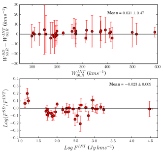
Figure 2: Upper panel: A comparison between $W_{50,R}$ derived from the single dish data $W_{50,R}^{SD}$ (EDD) and from the interferometric data $W_{50,R}^{INT}$, corrected for instrumental resolution. Lower panel: A comparison between the integrated flux derived from interferometric data and flux from the single–dish observations.

3.3 Global Hi profiles

The global Hi profile is one of the main data products of the Hi observations. It contains information about the gas content of a galaxy, while a galaxy’s rotation velocity can be estimated from the width of the profile. The Hi line profiles were obtained by measuring the primary beam corrected flux density within the masked area in each velocity channel. The errors on the flux densities were determined empirically by calculating the rms noise in the emission free regions of each channel map. Because features such as warps of the Hi disks or non–circular motions do not manifest themselves clearly and unambiguously in the global Hi line profile, we do not obtain a large variety of profile morphologies. Most of the global profiles of our sample galaxies are double–peaked, with the exception of three dwarf galaxies, which show boxy profile shapes: NGC 2366, IC 2574 and NGC 4605, as can be inferred from Table 4. However, some asymmetries in the profiles are still present and cause a difference in flux between the receding and approaching sides of a galaxy. The flux ratios between both sides of the global profiles can be found in Table 4. Based on these flux ratios, the different shapes of the global profiles were classified into 4 categories: symmetric, slightly asymmetric, asymmetric and boxy.

3.3.1 Integrated Hi fluxes

The integrated Hi flux was determined as the sum of the primary beam corrected flux densities in the channel maps, multiplied by the channel width: $\int S_{v}dv$   $[Jy\,kms^{-1}]$. The integrated fluxes for our sample galaxies are listed in Table 6. The error on the integrated flux was calculated as the square–root of the quadrature–sum of the errors on the flux densities in each velocity channel (see above).

In the bottom panel of Figure 2 we present a comparison of the integrated fluxes derived from the interferometric data and those from single–dish observations. The values of the fluxes from the single-dish measurements were taken from the “All Digital Hi catalog” (Courtois et al., 2009) as compiled in EDD (Tully et al., 2009). The details of the single–dish measurements can be found in Koribalski et al. (2004); Springob et al. (2005); Courtois et al. (2009, 2011); Haynes et al. (2011). The weighted mean difference of $-0.023\pm 0.009$ shows that there is no significant systematic difference between the single–dish and interferometric flux measurements. However, some individual galaxies do show a significant difference which can be explained in several ways. First, single–dish observations might be contaminated due to a contribution to the flux by nearby companion galaxies within the same beam and at the same recession velocity. Second, an interferometric measurement might miss flux in case the shortest baselines cannot properly sample the largest spatial structures of an Hi disk. Third, a single–dish measurement can miss flux due to the angular size of a galaxy on the sky. In particular, many of our nearby calibrator galaxies are much larger than the primary beam of the single-dish telescopes. Despite these complications in the flux measurements, the unweighted average difference between the single–dish fluxes from the literature and our interferometric fluxes is only marginal with slightly more flux recovered by the interferomentric observations. Consequently we conclude that our results are in good agreement with previous single–dish measurements. Note, however, that accurate flux measurements are not crucial for our purposes.

3.3.2 Line widths and rotational velocities

Observational studies of galaxies with single–dish telescopes allow the global Hi profiles to be collected for thousands of galaxies. These profiles hold information not only about the Hi gas content of galaxies, but also about their rotational velocities. The corrected width of the global Hi profile is a good estimator of the overall circular velocity of a galaxy, which is usually defined as 2V${}_{\rm circ}=W/\sin(i)$, where V_circ is usually associated with the maximum rotational velocity. The kinematic information provided by the global Hi profile, however, is not very accurate because it provides only a single value for the entire galaxy. The rotation curve of a galaxy, on the other hand, represents the circular velocity as a function of distance from a galaxy’s dynamical centre. As was already mentioned above, rotation curves of galaxies are not always flat and featureless, the circular velocity varies with distance from the dynamical centre of a galaxy. For instance, some galaxies show declining rotation curves where V_max, the maximal circular velocity of a rotation curve, will be larger than V_flat, the circular velocity of the outermost part of the Hi disk, which better probes the gravitational potential of the dark matter halo. The angular size of a spiral galaxy is usually not large enough to map its Hi velocity field point–by–point with a single–dish telescope, except for the very nearby, large galaxies in the Local Group (the LMC, SMC and M31). For most other galaxies, the ratio of the Hi diameter to the single–dish beam size is too small to obtain detailed rotation curves (e.g. Bosma (1978), chapter 3). However, the global Hi profile can give a rough estimate for the kinematics of a galaxy.

The shape of the global Hi profile can provide some indication for the shape of the rotation curve of a galaxy. For example, a double–peaked profile indicates that the gas disk of a galaxy is sufficiently extended to sample the flat part of a galaxy’s rotation curve, while a Gaussian or boxy shaped global profile is often observed for dwarf or low surface–brightness galaxies which usually have a slowly rising rotation curve with V_max$<$ V_flat. The wings or steepness of the edges of the profile can be an indication for a declining rotation curve with V_flat$<$ V_max, or for the presence of a warp (Verheijen, 2001). Our goal is to investigate for each sample galaxy how the circular velocity derived from the global Hi profile compares to the V_max and V_flat as measured from the rotation curve.

The width of the global profile is usually defined as a width in $kms^{-1}$ between the two edges of the profile at the 50% level of the peak flux density. However, different methods for defining the width of the profile exist in the literature. For instance the profile width can be measured at the 20% level, or by considering the mean peak flux density. In our case, for double–peaked profiles, the maximum flux densities of the two peaks were used separately to determine the full width of the profile at the 50% and 20% levels. In such a profile the high velocity peak represents the receding side of the galaxy and the low velocity peak the approaching side. Thus, the widths were calculated using the difference in velocities, corresponding to the 50% and 20% level of each peak of the profile separately:

$$W_{20,50\%}=V_{20,50\%}^{rec}-V_{20,50\%}^{app}.$$ (1)

In the other two cases where the profiles are not double–peaked, the overall peak flux was used to determine the 50% and 20 % levels. The systemic velocity was determined from the global profile as

$$V_{sys}^{GP}=0.25\,(V_{20\%}^{app}+V_{50\%}^{app}+V_{20\%}^{rec}+V_{50\%}^{rec}),$$ (2)

The adopted error on $V_{sys}^{GP}$ was calculated as half the difference between the values of $V_{sys}^{GP}$ based on the 20% and 50% levels separately.

All measured widths were corrected for instrumental broadening due to the finite instrumental velocity resolution. This correction depends on the instrumental velocity resolution and on the steepness of the profiles for which the Gaussian shape was assumed. For a detailed description of this method see Verheijen & Sancisi (2001).

Our results can be compared to the corrected widths of the profiles from single–dish telescopes taken from the literature sources mentioned above (see section 3.3.1). The upper panel of Figure 2 demonstrates the comparison between the widths at the 50% level derived from the interferometric measure and those from the literature (Koribalski et al., 2004; Springob et al., 2005; Courtois et al., 2009, 2011; Haynes et al., 2011). There is no systematic offset found and the data are in excellent agreement with the unweighted average difference of $0.031\pm 0.47$ $kms^{-1}$ with a 5 $kms^{-1}$ rms scatter. The measurements obtained from the global Hi profiles are presented in Table 4.

Name	$V_{sys}^{GP}$		$W_{50}$	$W_{20}$	Frec/Fapp	Shape
	$kms^{-1}$		$kms^{-1}$	$kms^{-1}$
NGC 0055	130$\pm$	16	185$\pm$4	201$\pm$6	2.74	A
NGC 0224	-297$\pm$	3	517$\pm$5	533$\pm$7	1.08	S
NGC 0247	161$\pm$	11	200$\pm$3	227$\pm$3	0.86	SA
NGC 0253	264$\pm$	20	410$\pm$3	419$\pm$5	0.93	S
NGC 0300	131$\pm$	10	160$\pm$5	167$\pm$1	0.82	S
NGC 0925	544$\pm$	6	200$\pm$8	228$\pm$9	1.08	SA
NGC 1365	1630$\pm$	13	380$\pm$10	405$\pm$7	1.87	A
NGC 2366	92$\pm$	15	100$\pm$10	120$\pm$11	1.38	B
NGC 2403	120$\pm$	15	225$\pm$1	257$\pm$4	0.63	A
NGC 2541	568$\pm$	8	200$\pm$6	211$\pm$6	0.76	SA
NGC 2841	641$\pm$	14	590$\pm$3	615$\pm$4	1.27	SA
NGC 2976	-7$\pm$	10	130$\pm$7	164$\pm$8	1.45	B
NGC 3031	-43$\pm$	13	415$\pm$6	425$\pm$7	1.06	SA
NGC 3109	410$\pm$	6	110$\pm$1	130$\pm$1	1.07	SA
NGC 3198	644$\pm$	12	315$\pm$4	322$\pm$1	1.21	S
IC 2574	40$\pm$	11	105$\pm$2	134$\pm$3	1.22	B
NGC 3319	748$\pm$	18	195$\pm$6	221$\pm$3	0.79	A
NGC 3351	761$\pm$	19	260$\pm$6	284$\pm$3	1.17	S
NGC 3370	1288$\pm$	8	275$\pm$4	301$\pm$6	0.91	SA
NGC 3621	714$\pm$	16	275$\pm$7	293$\pm$7	1.29	A
NGC 3627	706$\pm$	9	340$\pm$7	370$\pm$10	1.38	A
NGC 4244	258$\pm$	13	195$\pm$6	218$\pm$4	0.85	SA
NGC 4258	455$\pm$	10	420$\pm$6	434$\pm$7	0.91	SA
NGC 4414	730$\pm$	5	375$\pm$6	395$\pm$6	0.94	SA
NGC 4535	1945$\pm$	20	270$\pm$6	278$\pm$5	1.30	SA
NGC 4536	1781$\pm$	19	320$\pm$6	333$\pm$5	1.23	SA
NGC 4605	155$\pm$	5	150$\pm$15	186$\pm$5	0.58	A/B
NGC 4639	989$\pm$	11	275$\pm$6	290$\pm$11	0.94	S
NGC 4725	1230$\pm$	10	400$\pm$4	405$\pm$2	1.78	A
NGC 5584	1648$\pm$	8	190$\pm$10	197$\pm$2	0.74	A
NGC 7331	807$\pm$	8	500$\pm$10	527$\pm$1	1.12	SA
NGC 7793	216$\pm$	13	174$\pm$10	195$\pm$3	1.10	SA

Table 4: Measurements from the global Hi profiles. Column (1): galaxy name; Column (2): heliocentric systemic velocity; Column (3): global profile width at 50% level; Column (4): global profile width at 20% level; Column (5): ratio between integrated flux of receding and approaching side of a galaxy; Column (5):Shape of the profile: S–symmetric, SA–slightly asymmetric; A–asymmetric; B–boxy.

3.4 Velocity fields

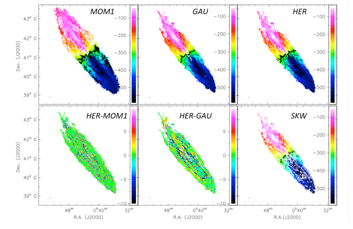
Figure 3: Upper panels from left to right: three types of velocity fields – Moment 1, Gaussian, and Gauss-Hermite velocity fields; Bottom panels from left to right: residual maps between Gauss-Hermite and Moment 1 velocity fields, Gauss-Hermite and Gaussian velocity fields, and the Gaussian velocity field with blanked skewed regions of the velocity profile. Data is shown for NGC 224.

After we estimated the rotational velocity of our sample galaxies using the width of global Hi profiles at the 50% and 20% levels, we need to compare these values with the velocities V_max and V_flat derived from the rotation curves of the galaxies. However, first the velocity field should be constructed for each galaxy, from which the rotation curve will be derived.

Velocity fields are playing a very important role in analysing the dynamics of the cold gas in a galaxy. Usually, the strongest signature of a velocity field reflects the rotation of the gas disk in the gravitational potential of a galaxy. In practice, however, velocity profiles are often affected by various systematic effects caused either by limited instrumental resolution or by physical processes within a galaxy.

The most common instrumental effect is known as “beam-smearing” which becomes manifest in observations with relatively low angular resolution (Bosma (1978), chapter 3). This usually happens when a synthesised beam is relatively large in comparison with the size of the galaxy, leading to asymmetries in the individual velocity profiles at different locations in the galaxy, in particular near its dynamical centre. The velocity profiles become skewed towards the systemic velocity of the galaxy and, thereby, the rotational velocity of the galaxy can be systematically underestimated. Therefore, one needs to correct for this effect by identifying the velocity close to the maximum velocity found in each velocity profile (Sancisi & Allen, 1979). Otherwise, the velocity obtained at a particular position will always be closer to the systemic velocity of the galaxy. Even though our sample consists of very large, nearby galaxies, three of the galaxies observed with the GMRT (NGC 3370, NGC 4639, NGC 5584) show “beam-smearing” features in their velocity profiles (see Appendix A for more details). For those galaxies we use the envelope–tracing correction method described in Verheijen & Sancisi (2001).

Furthermore, physical processes within a galaxy can have important effects on the observed velocity field and may lead to non–axisymmetries and non–circular motions of the gas. Usually these processes are associated with gas flows induced by the gravitational potential of spiral arms and/or bars of galaxies, and result in so–called streaming motions (Visser, 1980; Shetty et al., 2007). These appear as coherent deviations from the circular velocity of the gas in a galaxy. Since we are interested in measuring the circular velocity of the gas to probe the gravitational potential of the dark matter halo, the flat part of the outer rotation curve V_flat should be measured accurately. Therefore we identified and removed the signature of streaming motions from the velocity fields. There are many ways to construct velocity fields, and below we describe the most common of them, as well as our method of identifying streaming motions.

Calculating the first moment of the velocity profiles is one of the most well–known and computationally straight forward methods to construct a velocity field. Here the velocity at each position in the velocity field is an intensity weighted mean of the pixel values along the operation axis in the data cube. Despite it being the most commonly used approach, this method has many disadvantages and its sensitivity to noise peaks in a Hi spectrum is one of them. To obtain a reliable velocity field one needs to be very careful in identifying the emission regions and use only those areas to prevent the noise from significantly influencing the mean velocity. Another disadvantage is the fact that a first moment can be sensitive to the effects of severe beam–smearing which may result in skewed profiles. Thus, first–moment velocity fields can be used only as a first order approximation or as initial estimates for the other methods. The upper left panel of Figure 3 illustrates a moment–1 velocity field of NGC 224.

Fitting a Gaussian function to the velocity profiles is another way to derive the velocities that are representative of the circular motion of the gas. The central velocity of the Gaussian component defines the velocity at each position in the velocity field. Where the first–moment method always yields a velocity regardless of the signal–to–noise ratio in the profile, fitting a Gaussian to the profile requires a minimum signal–to–noise ratio. Therefore, a velocity field constructed by Gaussian fits usually constitutes of fewer pixels that have a higher reliability compared to a first–moment map. In spite of the fact that a Gaussian–based velocity field is usually more sparse, this method is most common to construct reliable Hi velocity fields for detailed analyses. The upper–middle panel of Figure 3 shows a Gaussian–based velocity field of NGC 224, illustrating that velocity profiles at lower signal–to–noise ratio in the outer regions of galaxies do not allow for acceptable Gaussian fits.

Using a Gauss–Hermite polynomial function to fit the velocity profiles allows the identification of asymmetric velocity profiles that may be affected by beam–smearing and/or streaming motions and that cannot be described properly by a single Gaussian. Gauss–Hermite polynomials allow to quantify deviations from a Gaussian shape with two additional parameters describing the skewness ($h3$ term) and kurtosis ($h4$ term) of the profile (van der Marel & Franx, 1993). In our case we do not take into account the $h4$ term because instrumental and astrophysical effects typically result in asymmetric velocity profiles that can be identified by their $h3$ values.

For our studies we used both Gaussian and Gauss–Hermite polynomial functions to fit the velocity profiles and construct the corresponding velocity fields as indicated by GAU and HER in Figure 3. We identify asymmetric velocity profiles by considering the difference between the HER and GAU velocity fields as illustrated in the bottom–middle panel of Figure 3. Pixels with values in excess of $\pm 3$ km/s in the HER$-$GAU difference map were blanked in the GAU velocity field. Thereby we have obtained the third type of velocity field SKW as illustrated in the bottom–right panel of Figure 3. These SKW velocity fields will be used to derive the rotation curves from.

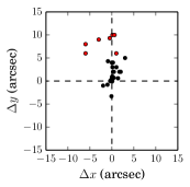
Figure 4: Differences between optical and dynamical centres of our sample galaxies. Red symbols indicated the outliers for which optical centres were adopted during the tilted–ring modelling.

Figure 5: Upper panel: the differences between optical position angles from TC12 and the kinematical position angles derived from the tilted–ring modelling. Bottom panel: the differences between the optical inclination angles from TC12 and the kinematical inclination angles derived from the tilted–ring modelling.

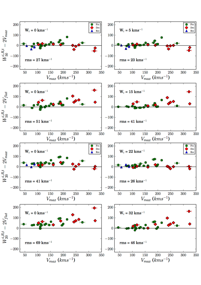
Figure 6: Comparison of the global profile widths at the 50% level (upper four panels) and the 20% level (lower four panels), corrected only instrumental resolution and inclination $W_{50,20}^{R,i}$ with 2V_max and 2$V_{\rm flat}$ (left panels), and corrected also for random motions $W_{50,20}^{R,t,i}$ (right panels). Blue symbols indicate galaxies with rising rotation curves (V_max$<$V_flat) and red symbols indicate galaxies with declining rotation curves (V_max$>$V_flat). Green symbols show flat rotation curves without declining part (V_max$=$V_flat).

Name	$V_{sys}$		$P.A.$		$Incl.$		$V_{max}$		$V_{flat}$
	$kms^{-1}$		$deg.$		$deg.$		$kms^{-1}$		$kms^{-1}$
NGC 0055	130$\pm$	5	110$\pm$	3	78$\pm$	7	85$\pm$	1	85$\pm$2
NGC 0224	-300$\pm$	3	37$\pm$	1	78$\pm$	1	261$\pm$	2	230$\pm$7
NGC 0247	160$\pm$	10	169$\pm$	3	77$\pm$	2	110$\pm$	5	110$\pm$5
NGC 0253	240$\pm$	5	230$\pm$	2	77$\pm$	1	200$\pm$	4	200$\pm$4
NGC 0300	135$\pm$	10	290$\pm$	3	46$\pm$	6	103$\pm$	3	85$\pm$7
NGC 0925	550$\pm$	5	283$\pm$	2	61$\pm$	5	115$\pm$	4	115$\pm$4
NGC 1365	1640$\pm$	3	218$\pm$	2	39$\pm$	8	322$\pm$	6	215$\pm$4
NGC 2366	107$\pm$	10	42$\pm$	6	68$\pm$	5	45$\pm$	5	45$\pm$5
NGC 2403	135$\pm$	1	124$\pm$	1	61$\pm$	3	128$\pm$	1	128$\pm$1
NGC 2541	560$\pm$	5	170$\pm$	3	64$\pm$	4	100$\pm$	4	100$\pm$4
NGC 2841	640$\pm$	20	150$\pm$	3	70$\pm$	2	325$\pm$	2	290$\pm$6
NGC 2976	5$\pm$	5	323$\pm$	1	61$\pm$	5	78$\pm$	4	78$\pm$4
NGC 3031	-40$\pm$	10	330$\pm$	4	59$\pm$	5	249$\pm$	3	215$\pm$9
NGC 3109	404$\pm$	5	92$\pm$	3	80$\pm$	4	57$\pm$	2	–
NGC 3198	660$\pm$	10	215$\pm$	5	70$\pm$	1	161$\pm$	2	154$\pm$4
IC 2574	51$\pm$	3	55$\pm$	5	65$\pm$	10	75$\pm$	5	–
NGC 3319	730$\pm$	4	33$\pm$	2	57$\pm$	4	112$\pm$	10	112$\pm$10
NGC 3351	780$\pm$	5	192$\pm$	1	47$\pm$	5	190$\pm$	5	176$\pm$8
NGC 3370	1280$\pm$	15	327$\pm$	3	55$\pm$	5	152$\pm$	4	152$\pm$4
NGC 3621	730$\pm$	13	344$\pm$	4	65$\pm$	7	145$\pm$	5	145$\pm$5
NGC 3627	715$\pm$	10	172$\pm$	1	58$\pm$	5	183$\pm$	7	183$\pm$7
NGC 4244	245$\pm$	3	222$\pm$	1	88$\pm$	3	110$\pm$	6	110$\pm$6
NGC 4258	445$\pm$	15	331$\pm$	1	72$\pm$	3	242$\pm$	5	200$\pm$5
NGC 4414	715$\pm$	7	160$\pm$	2	52$\pm$	4	237$\pm$	10	185$\pm$10
NGC 4535	1965$\pm$	5	180$\pm$	1	41$\pm$	5	195$\pm$	4	195$\pm$4
NGC 4536	1800$\pm$	6	300$\pm$	3	69$\pm$	4	161$\pm$	10	161$\pm$10
NGC 4605	160$\pm$	15	293$\pm$	2	69$\pm$	5	87$\pm$	4	–
NGC 4639	978$\pm$	20	311$\pm$	1	42$\pm$	2	188$\pm$	1	188$\pm$1
NGC 4725	1220$\pm$	14	30$\pm$	3	50$\pm$	5	215$\pm$	5	215$\pm$5
NGC 5584	1640$\pm$	6	152$\pm$	4	44$\pm$	4	132$\pm$	2	132$\pm$2
NGC 7331	815$\pm$	5	169$\pm$	3	75$\pm$	3	275$\pm$	5	275$\pm$5
NGC 7793	228$\pm$	7	290$\pm$	2	50$\pm$	3	118$\pm$	8	95$\pm$8

Table 5: Tilted–ring modeling results. Column (1): galaxy name; Column (2): systemic velocity; Column (3): kinematic position angle, calculated as an angle between the North direction and receding side of a galaxy; Column (4): kinematic inclination from face–on; Column (5): maximal rotational velocity; Column (6): rotational velocity of the flat part of rotation curve.

3.5 Rotation curves and velocity field models

From the previous section it is clear that velocity fields tend to have pixels with skewed velocity profiles mostly due to beam–smearing and non–circular motions. Thus it is important to stress that we derive rotation curves for our galaxies from the SKW velocity fields which were censored for such effects (see Section 3.4). For this purpose, we fitted a tilted–ring model to the SKW velocity field to derive the rotation curve of each galaxy. Details on the tilted–ring modelling method, its parameter fitting and error calculations, are described by (Begeman, 1989). The derivation of a rotation curve was done in four steps. The widths of the tilted–rings were adjusted separately for each galaxy, taking into account the Hi morphology and the size of the synthesised beam.

As a first step, for each ring we fitted to the SKW velocity field, only the position of its dynamical centre $x_{0}$ and $y_{0}$, and the systemic velocity of a galaxy $V_{sys}$ were fitted. All other parameters, such as the position angle ($pa$), inclination angle ($i$) and the rotation velocity V_rot were fixed and remained the same for all tilted rings. In this first step, the position ($pa$) and inclination ($i$) angles were adopted from the optical measurements done by TC12 and listed in Table 1 while $V_{rot}$ was estimated from the measured width of the global Hi profile. All the data points within a tilted ring were weighted uniformly at this step. After the fitting, the position of the dynamical centre ($x_{0},y_{0}$) and the systemic velocity $V_{sys}$ were calculated as the weighted means of the solutions for all fitted rings. For cases where the fitted position of the dynamical centre had large deviations from ring to ring, the position of the optical centre was adopted. The offsets between optical and dynamical centres are shown in Figure 4 and are typically smaller than the angular size of the interferometric synthesised beam.

At the second step, we fitted only the position angle ($pa$) of a tilted ring, indicating the angle between north and the kinematically receding side of a galaxy, measured eastward. All the other parameters were kept fixed whereby the position of the dynamical centre and the systemic velocity $V_{sys}$ were adopted from the previous step. Again, all the data points within each tilted–ring were weighted uniformly. While the position angle can be determined very accurately and is mostly invariant from ring to ring, we paid attention to the possible existence of a trend with radius so as to include a geometric warp in the model when warranted. The weighted average value of the position angle within the optical radius of a galaxy, as well as a possible trend with radius were fixed at the next step. A comparison between the optical and the kinematical position angles is presented in Figure 5a. Overall, the optical and kinematic position angles are in a good agreement with a weighted mean difference of $-0.5\pm 0.8$ degrees.

In the third step, adopting and fixing the results from the previous steps, we fitted both the inclination angle ($i$) and the rotational velocity (V_rot) of each ring, weighing all the data points in a ring according to $cos(\theta)$, where $\theta$ is the angle in the plane of the galaxy measured from its receding side. The values of the inclination angle and the rotation velocity of a tilted–ring are highly covariant in the fitting algorithm and rather sensitive to pixel values in the SKW velocity field that are still affected by non–circular motions. Hence, the fitted inclination may vary significantly from ring to ring within a galaxy. We assume, however, that the cold gas within the optical radius of a galaxy is largely co–planar and we calculated the weighted mean inclination of the rings within the optical radius of the galaxy. We refer to this as the kinematic inclination of a galaxy. If the more accurately determined position angle indicates a warp in the outer regions, we also allow for an inclination warp if the fitted values hint at this. Adopting the inclination angles derived from the optical images as reported by TC12, we compare the optical and kinematic inclination angles in the bottom panel of Figure 5. We find that the kinematical inclination angles are systematically lower than the optical ones, with an average weighted difference of $2.06\pm 0.81$ degrees. It is important to point out that the derived optical inclination angles depend on the assumed thickness of the stellar disk when converting isophotal ellipticities to inclinations, and therefore it can cause the systematic offset between optical and kinematical inclinations. Such a systematic bias is not expected in deriving kinematic inclinations. We note that the systematic difference we find is very close to an empirical correction of 3^∘ as determined by Aaronson et al. (1980), which was usually applied when interpreting optical and kinematical inclination angles.

In the fourth and final step, V_rot was fitted for each tilted–ring while all the previously determined parameters ($x_{0},y_{0},V_{sys},pa_{kin},i_{kin}$) were kept fixed, including the geometry of a possible warp. Hence, in deriving the rotation curve of a galaxy we use its global systemic velocity and geometry (except for the five cases where optical centres were adopted, Figure 4) based on the characteristics of the SKW velocity field. The values of V_rot as measured during the previous step were adopted as an initial estimate while all the points within each tilted–ring were considered and weighted with $cos(\theta)$ when fitting V_rot for each ring, yielding the circular velocity of the HScience gas as a function of distance from a galaxy’s dynamical centre. To investigate possible kinematic asymmetries we fitted V_rot not only to the full tilted–ring but also to the receding and approaching sides of a galaxy separately. Subsequently, we used these rotation curves to identify the maximum circular velocity V_max of the gas disk, as well as the circular velocity of the outer gas disk V_flat.

To verify our final rotation curves, they were projected onto position–velocity diagrams extracted from the data cubes for visual inspection. To further verify the results from the tilted–ring fits to the SKW velocity field, they were also used to construct an axisymmetric, model velocity field of a regular, rotating gas disk. This model was subsequently subtracted from the Gauss–Hermite polynomial velocity field to construct a map of the residual velocities. This residual velocity field highlights the locations of velocity profiles with significant skewness and could have revealed possible systematic residuals that should have been accommodated by the tilted–ring model.

Table 5 summarises the final results obtained from the tilted–ring fitting process based on the SKW velocity field. Errors on $V_{sys}$, the position angle and the inclination are based on the variance in the ring–to–ring solutions. Errors on V_max and V_flat were measured as the difference between the velocities of the approaching and receding sides of the galaxy. All final data products are presented in the accompanying Atlas that will be discussed below.

We conclude this section by recalling that the global geometric properties of the Hi gas disks (dynamical centre, position angle and inclination angle) as derived from the SKW velocity fields are in good agreement with the same geometries derived from photometric images of these galaxies. Moreover, from the fitting procedure we derived high–quality rotation curves of the cold gas, presenting the circular velocity of a galaxy as a function of distance from its dynamical centre. These rotation curves will be used in a forthcoming paper analysing the detailed mass distributions within our sample galaxies. For the purpose of studying the statistical properties of the Tully–Fisher relation in a forthcoming paper, we measure two values of the rotational velocity of each galaxy: the maximal rotational velocity V_max and the velocity at the flat part of the outer rotation curve V_flat. In the next section we will compare these values with the rotational velocity as estimated from the corrected width of the single–dish profiles.

Figure 7: Correlation between Hi mass and isophotal diameter of the Hi disks. The solid line indicates the linear fit to the relation. Dashed and dashed–dot lines show the results found by Verheijen & Sancisi (2001) and by Martinsson (2011), respectively.

3.6 Comparison of different velocity measures

As was already mentioned above, the width of the global Hi profile can give a good estimate of the typical circular velocity of the cold gas in a galaxy. However the measured width of the global profile should be corrected not only for finite instrumental spectral resolution, but also for astrophysical effects such as the turbulent motions of the gas and the inclination of the rotating gas disk.

3.6.1 Turbulent motion correction.

The empirical correction of the measured line width for turbulent motion of the gas was investigated previously by several authors (Bottinelli et al., 1983; Broeils, 1992; Rhee & van Albada, 1996) by matching the corrected global Hi line widths to the rotational velocities as measured from rotation curves.

In this work we adopt the recipe and parameter values for turbulent motion correction from Verheijen & Sancisi (2001). While adopting $W_{c}=120$ km/s, they showed that, in order to match the amplitudes of the rotation curves, the empirical values of the turbulence parameter $W_{t}$ as proposed in previous studies, should be adjusted. Its values depend on the level at which the line width was measured (20% or 50%) and on the velocity measure from the rotation curve (V_max or V_flat). Therefore, when applying this correction to our galaxies, we adopt their values:

$W_{t,20}^{max}=22\,kms^{-1},\,W_{t,50}^{max}=5\,kms^{-1}$;

$W_{t,20}^{flat}=32\,kms^{-1},\,W_{t,50}^{flat}=15\,kms^{-1}$.

3.6.2 Inclination correction.

The correction of the global profile width for inclination was done using the kinematic inclinations obtained from the tilted–ring modelling of the SKW velocity fields as listed in Table 5:

$W_{50,20}^{R,t,i}=W_{50,20}^{R,t}/\,sin(i_{kin})$.

The line widths corrected for instrumental resolution, turbulent motion, and inclination are presented in Table 6.

3.6.3 Comparing $W_{50,20}^{R,t,i}$, V_max and V_flat

We start this subsection by stressing, again, that a single–dish measurement of a global Hi profile does not inform the observer whether a galaxy’s rotation curve is declining or not.

Figure 6 shows the differences between the corrected global profile widths and the values of V_max and V_flat derived from the rotation curves. Green symbols correspond to galaxies with rotation curves that monotonically rise to a extended flat part (V_max = V_flat). Red symbols correspond to galaxies with rotation curves that rise to a maximum beyond which they decline to a more or less extended flat part (V_max$>$V_flat). Blue symbols correspond to galaxies with rotation curves that are still rising at theit last measured point and do not reach a flat part (V_max$<$V_flat while V_flat is not actually measured). The left panels show the differences without any random motion corrections ($W_{t}=0$) applied, and the right panels show the differences with the random motion corrections applied for variouss values of $W_{t}$.

We see that the more–massive galaxies tend to have declining rotation curves while the three galaxies with rising rotation curves are all of low mass. From the panels in the left column we conclude that the global profile width systematically overestimates the rotational velocity if no correction for turbulent motions is applied, with the exception of $W_{50}^{R,i}$ as an estimate for 2V_max (upper panel). Furthermore, by comparing the corresponding panels in the left and right columns, we see that the variance in the differences is significantly reduced by applying the corrections for turbulent motions: Both $W_{50}^{R,t,i}$ and $W_{20}^{R,t,i}$ match the maximum velocity notably better after corrections for random motions, although systematic offsets between the red and green symbols persist.

Focusing on the panels in the right column, we see that $W_{t}$ values of 5 and 22 km/s allow the recovery of 2V_max from the 50% and 20% line widths respectively, at least in a statistical sense. In these cases, however, 2V_flat for galaxies with monotonically rising rotation curves (green symbols) tend to be systematically overestimated, especially for the 20% line widths $W_{20}^{R,t,i}$. We also see that $W_{t}$ values of 15 and 32 km/s allow a somewhat better recovery of 2V_flat for galaxies with monotonically rising rotation curves (green symbols) but the corrected global profile line widths systematically overestimate V_flat for galaxies with declining rotation curves due to the fact that V_max$>$V_flat.

An important conclusion from this comparison is that, for a sample of galaxies with flat and declining rotation curves, the corrected width of the global Hi line profile cannot be unambiguously corrected to recover V_flat which is probing the potential of the dark matter halo without introducing a systematic bias that is largely correlated with the mass of a galaxy. This has implications for the slope of, and may possibly introduce a curvature in, the Tully–Fisher relation when using $W_{20,50}^{R,t,i}$ from global Hi profiles instead of V_flat from extended Hi rotation curves.

Name	$\int S_{v}dv$		$M_{HI}$		$D_{HI}$		$\Sigma_{HI}^{max}$
	Jy $kms^{-1}$		$10^{9}M_{\odot}$		$kpc$		$M_{\odot}pc^{-2}$
NGC 0055	1786.	7	1.	54	20.	3	14.	7
NGC 0224	30292.	5	4.	18	44.	5	5.	4
NGC 0247	594.	4	1.	67	26.	7	6.	1
NGC 0253	693.	7	1.	95	25.	1	4.	6
NGC 0300	1779.	2	1.	57	28.	1	5.	6
NGC 0925	274.	7	5.	44	35.	5	4.	4
NGC 1365	167.	3	12.	71	57.	4	7.	8
NGC 2366	307.	1	0.	79	19.	2	12.	3
NGC 2403	1088.	6	2.	61	30.	9	9.	4
NGC 2541	143.	3	4.	25	32.	6	1.	6
NGC 2841	183.	5	8.	56	68.	1	4.	3
NGC 2976	50.	2	0.	15	5.	1	12.	1
NGC 3031	907.	1	2.	77	34.	8	4.	1
NGC 3109	1181.	2	0.	47	12.	6	7.	1
NGC 3198	218.	2	9.	81	66.	9	4.	9
IC 2574	389.	4	1.	34	27.	7	8.	0
NGC 3319	93.	1	3.	88	29.	1	1.	4
NGC 3351	59.	9	1.	68	31.	7	6.	4
NGC 3370	17.	3	2.	90	28.	4	4.	9
NGC 3621	904.	1	10.	05	51.	0	9.	3
NGC 3627	53.	7	1.	27	19.	4	11.	3
NGC 4244	423.	9	1.	77	20.	3	1.	2
NGC 4258	440.	4	5.	55	35.	4	4.	8
NGC 4414	25.	2	1.	86	18.	8	2.	0
NGC 4535	75.	7	4.	44	38.	2	5.	1
NGC 4536	82.	2	4.	40	36.	5	6.	2
NGC 4605	55.	1	0.	36	6.	7	3.	1
NGC 4639	13.	8	1.	56	21.	2	4.	3
NGC 4725	102.	2	3.	92	80.	4	2.	6
NGC 5584	15.	9	1.	93	24.	2	5.	1
NGC 7331	202.	1	10.	03	42.	8	22.	1
NGC 7793	352.	5	1.	29	15.	2	10.	4

Table 6: Measured Hi properties. Column (1): galaxy name; Column (2): integrated Hi flux; Column (3): Hi mass; Column (4): Hi diameter; Column (5): maximum Hi column density, projected towards face-on

3.7 Total Hi maps and radial Hi surface–density profiles

Hi integrated column–density maps were created by adding the primary beam corrected, non–zero emission channels of the cleaned data cubes with applied masks. The pixel values in the resulting map were converted from flux density units $[Jy/beam]$ to column–densities $[atoms$ $cm^{-2}]$, according to the formula:

$$N_{HI}=1.823\times 10^{18}\int T_{b}dv,$$ (3)

where $T_{b}$ is the brightness temperature and $dv$ is the velocity width over which the emission was integrated. $T_{b}$ in Kelvin is calculated as follows:

$$T_{b}=\frac{605.7}{\Theta_{x}\Theta_{y}}\,S_{\nu}\,\bigg{(}\cfrac{\nu_{0}}{\nu}\bigg{)}^{2},$$ (4)

where $\Theta_{x}$ and $\Theta_{y}$ are the major and minor axes of the Gaussian beam in arcseconds, $S_{\nu}$ is the flux density in $mJy/beam$, and $\nu_{0}/\nu$ is the ratio between the rest–frame and observed frequency of the Hi line.

The radial Hi surface density profiles were derived by azimuthally averaging pixel values in concentric ellipses projected onto the Hi column–density map for both the receding and approaching side of a galaxy separately. The position and inclination angles of the ellipses were taken from the tilted–ring fitting results (see Section 3.5), taking a warp, if present, into account. Note that the column–density profiles are deprojected to represent face–on values. Subsequently the conversion from $[atoms$ $cm^{-2}]$ to $[M_{\odot}pc^{-2}]$ was applied:

$$1[M_{\odot}\,pc^{-2}]=1.249\times 10^{20}[atoms\,cm^{-2}].$$ (5)

The Hi column–density maps and the radial, face–on surface density profiles are presented in the Atlas while the azimuthally averaged peak column–density of each galaxy is listed in Table 6.

4 Global Hi properties

In this section we investigate the global properties of the gas disks of our sample galaxies and compare these to the same properties of galaxies in the volume–limited Ursa Major sample (Verheijen & Sancisi, 2001) and the sample of (Martinsson, 2011). Although our sample of Tully–Fisher calibrator galaxies is by no means statistically complete, it is important to demonstrate that our sample is not biased and representative of late–type galaxies, at least from an Hi perspective. The main properties of the Hi gas disks of our galaxies are listed in Table 6.

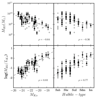
Figure 8: Upper panels: correlation between Hi mass and absolute K_s magnitude (left) and morphological type (right). For comparison, we show these values also for galaxies in the Ursa Major volume–limited sample from Verheijen & Sancisi (2001). Lower panels: correlation between Hi mass–to–light ratio and absolute K_s magnitude (left) and morphological type (right). Black dashed lines are fits to the relations with $\rho$ indicating Pearson’s correlation coefficient. Solid grey line show the fit to the Ursa Major sample.

4.1 The masses and sizes of Hi disks

The masses and sizes of Hi disks are among the main global parameters of spiral galaxies. A remarkably tight correlation exists between the mass and the size of a galaxy’s Hi disk as demonstrated before by various authors (Verheijen & Sancisi, 2001; Swaters et al., 2002; Noordermeer, 2006), although the slope and zero point of this correlation vary slightly from sample to sample. Here we investigate whether the galaxies in our sample adhere to this tight correlation.

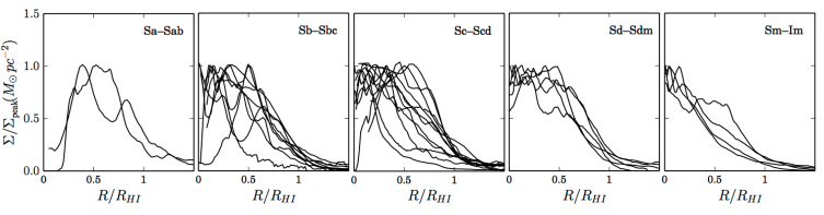
Figure 9: Azimuthally averaged Hi surface–density profiles, scaled in radius by $R_{HI}$ measured at $1\,M_{\odot}\,pc^{-2}$ and in amplitude by the peak surface–density. The profiles are presented in five bins of morphological types.

The total Hi mass of each galaxy is calculated according to:

$$M_{HI}\,[M_{\odot}]=2.36\times 10^{5}\,D^{2}\,\int S_{\nu}dv,$$ (6)

where $D$ is the distance to a galaxy in [Mpc], as listed in Table 1, and $\int S_{\nu}dv\,[Jy\,kms^{-1}]$ is the integrated flux density, as presented in Table 6 and described in Section 3.3.1.

Next, we measure the diameters of the Hi disks. We do not measure $D_{HI}$ from the Hi maps, which are often irregular in their outer regions. Instead, we measure the Hi radius as the radius where the azimuthally–averaged, face–on Hi surface–density has dropped to $1\,M_{\odot}\,pc^{-2}$.

The $M_{HI}$ versus $D_{HI}$ correlation for our sample galaxies is shown in Figure 7. The solid line illustrates a linear fit and can be described as:

$$log(M_{HI})=1.62log(D_{HI})+7.06,$$ (7)

with a rms scatter of 0.13. The dashed and dashed–dot lines correspond to the relations found by Verheijen & Sancisi (2001) and by Martinsson (2011), respectively. We find an insignificantly shallower slope for this correlation which may be due to a relatively small number of intrinsically small galaxies in our sample.

4.2 Hi mass versus luminosity and Hubble type

It is well known that Hi masses and $M_{HI}/L$ ratios of galaxies correlate well with the luminosity and morphological type of a galaxy. Our galaxy sample is not an exception and shows good agreement with previous studies (Roberts & Haynes, 1994; Verheijen & Sancisi, 2001; Swaters et al., 2002). In our work we consider the Hi masses and $M_{HI}/L_{Ks}$ ratios, and compare the trends observed in our sample with the volume–limited sample of Ursa Major galaxies (Verheijen & Sancisi, 2001) for which deep $K_{s}$ photometry is available and obtained in a similar fashion as for our sample galaxies, as will be discussed in a fortcoming paper.

Correlations of the total Hi mass and the Hi mass–to–light ratio with $M_{Ks}$ and the morphological types of the galaxies are shown in Figure 8. The light–gray symbols correspond to galaxies in the Ursa Major reference sample.

We see that our sample galaxies follow the same known correlations with a similar scatter as the reference sample. The upper–left panel of Figure 8 shows that more luminous galaxies tend to contain more Hi gas (Pearson’s correlation coefficient $\rho=-0.64$ ), while the lower–left panel shows that the Hi mass–to–light ratio decreases with luminosity ($\rho=0.83$). The upper–right panel of Figure 8 illustrates that a weaker trend exists between a galaxy’s Hi mass and its Hubble type, both for our sample galaxies ($\rho=-0.36$) and the Ursa Major reference sample ($\rho=-0.38$). The lower–right panel of Figure 8, however, presents a strong correlation between Hi mass–to–light ratio and Hubble type with later–type galaxies containing more gas per unit luminosity ($\rho=0.77$).

We conclude that the galaxies in our TFr calibrator sample are representative of normal field galaxies as found in a volume–limited sample.

4.3 Radial surface density profiles

As can be seen in Figure 1, our sample covers a broad range of morphological types from $Sa$ to Irregular. We divide our sample into five bins of morphological types $Sa-Sab$, $Sb-Sbc$, $Sc-Scd$, $Sd-Sdm$ and $Sdm-Im$ and investigate possible difference between the Hi surface density profiles of galaxies of different morphological types.

The azimuthally averaged radial Hi surface–density profiles, normalised to their peak values and their Hi diameters, are presented in Figure 9. Clearly the shapes and amplitudes of the profiles are very diverse, and cannot be described with a uniform profile, in disagreement with the results by Martinsson (2011) for the Disk–Mass sample which is dominated by $Sc$–type galaxies. Although there is a large variety in profile shapes, we confirm the overall trend that early–type spiral galaxies tend to have central holes in their Hi disks while late–type and irregular galaxies tend to have central concentrations of Hi gas. The gas disks of spiral galaxies of intermediate morphological types have a more constant surface–density or may show mild central depressions in their surface–densities

5 Summary

We have presented the analysis of 21-cm spectral–line aperture synthesis observations of 32 spiral galaxies, which are representing a calibrator sample for studying the statistical properties of the Tully–Fisher relation. The data were collected mostly from the literature and obtained with various observational facilities (VLA, ATCA, WSRT). We observed for the first time three galaxies in our sample ourselves with the GMRT. The most important aspect of this work is that, despite the broad range in data quality, we analysed the entire sample in the same manner. Although previously many of these galaxies were studied individually, we present for the first time a set of Hi synthesis imaging data products for all these galaxies together, analysed in a homogeneous way. The data products consist of total Hi maps, velocity fields in which asymmetric velocity profiles are identified and removed, Hi global profiles, radial Hi surface–density profiles, position–velocity diagrams and, most importantly, high–quality extended Hi rotation curves, all presented in an accompanying Atlas. The rotation curves and the derived measurements of V_max and V_flat will be used in forthcoming papers investigating the statistical properties of the Tully–Fisher relation. The radial Hi surface–density profiles will be used for rotation curves decompositions, aimed at studying the mass distributions within spiral galaxies.

Overall, our kinematical study of the gas disks of our sample galaxies shows excellent agreement with previously reported values for the position and inclination angles, and systemic velocities. We find a good agreement with literature values for both Hi fluxes and the widths of the global Hi profiles at the 50% level, obtained from single–dish observations. However, in some cases we find somewhat larger fluxes than previously reported in the literature (see Section 3.3.1 for details). This can be easily explained given the large angular size of our galaxies, and the fact that single–dish observations can miss some flux due to the relatively small beam sizes.

All galaxies in our sample have extended Hi disks, which serve our purpose to probe the gravitational potential of their dark matter halos. Moreover, our galaxies follow the well–known correlation between their Hi mass and the diameter of their Hi disks, but with a slightly shallower slope then shown in previous studies. Studies of the Hi mass and its correlation with the absolute $K_{s}$ magnitude show that while more luminous galaxies tend to have more Hi gas, its fraction decreases with luminosity. We find hints for similar trends with Hubble–type: late–type spiral galaxies tend to have a larger fraction of Hi gas than more early–type spirals, but the total mass of the Hi gas decreases. A qualitative comparison with the volume–limited sample of Ursa Major galaxies shows that our calibrator sample is respresenatative for a population of field galaxies.

The radial Hi surface–density profiles were scaled radially with $R_{HI}$ and divided into five groups according to the morphological type of the galaxies. The gas disks of early–type spirals tend to have central holes while the has disks of late–type spirals and irregulars tend to be centrally concentrated.

Velocity fields were constructed by fitting Gaussian and Gauss–Hermite polynomial functions to the velocity profile at each position in the data cube. We identified the pixels with skewed velocity profiles, using the difference between these two velocity fields, and censored them in the Gaussian velocity field, thereby creating a third type of velocity field.

Rotation curves were derived from these censored velocity fields using tilted–ring modelling. The procedure was done in four steps, which allowed to follow the geometry of a possible warp in the outer region. Rotation curves were identified into 3 categories: rising, flat and declining. The obtained values of V_max and V_flat were compared with the velocities derived from the corrected Hi global profiles at the 50% and 20% level. The comparison tests show that while the width of the Hi profile can be a good representation for the maximal rotation velocity of the galaxy, it may significantly overestimate the velocity at the outer, flat part of the rotation curve, especially for high–mass galaxies which tend to have declining rotation curves. For the rising rotation curves, where V_max is lower than V_flat, the width of the profile tends to underestimate V_flat.

The statistical properties of the Tully-Fisher relation based on different velocity measures ($W$, V_max and V_flat) will be studied in forthcoming papers.

Appendix A Notes on individual galaxies

NGC 55 : This galaxy is morphologically and kinematically asymmetric, with the receding side extending farther into the halo than the approaching side. It was previously studied by Puche et al. (1991) and Westmeier et al. (2013).

NGC 224 : The central region of this galaxy is lacking Hi gas and thus the rotation curve could not be constructed in the inner regions which is indicated by the vertial, dashed line in the rotation curve panel at a radius of 1500 arcsec. The rotation curve is declining. These data were first presented in Braun et al. (2009) and an alternative kinematic analyses can be found in Corbelli et al. (2010).

NGC 247 : This galaxy was previously studied by Carignan & Puche (1990).

NGC 253: This galaxy has a lack of Hi gas in its centre. The inner points of the rotation curve suffer from beam smearing, therefore the rotation curve is not properly recovered in the centre. The region affected by beam–smearing is indicated with a vertical, dashed line at a radius of 150 arcsec. It was previously studied by Puche et al. (1991).

NGC 300: This galaxy has a very extended Hi disk in comparison with the stellar disk, and is warped in position angle. Traces of Galactic emission can be seen at the zero–velocity channels in the position–velocity diagrams. The rotation curve is declining. It was previously studied by Puche et al. (1990) and Westmeier et al. (2011).

NGC 925: This galaxy has an extended Hi low surface–density disk. It was previously studied by Pisano et al. (1998) and as part of the THINGS survey (de Blok et al., 2008; Walter et al., 2008).

NGC 1365: A grand–design spiral galaxy with a strong bar. The central regions are completely dominated by non–circular motions due to the bar, and suffer from a lack of Hi gas for a proper recovery of the inner rotation curve. A warp can be identified in both position angle and inclination. It was previously studied by Jörsäter & van Moorsel (1996) and re-analysed lately by Zánmar Sánchez et al. (2008).

NGC 2366: This flocculent, barred galaxy is kinematically lopsided. It was previously studied as a part of the THINGS survey (de Blok et al., 2008; Walter et al., 2008; Oh et al., 2008).

NGC 2403: This galaxy was previously studied by Begeman (1987) and is part of the THINGS survey (de Blok et al., 2008; Walter et al., 2008).

NGC 2541: The Hi disk of this galaxy displays a warp in position angle.

NGC 2841: This galaxy has an extended, warped gas disk with a declining rotation curve. It was previously studied by Bosma (1981); Begeman (1987) and is a part of the THINGS survey (de Blok et al., 2008; Walter et al., 2008).

NGC 2976: This galaxy has an extended very low surface–density Hi disk. It has a solid–body rotation curve which does not reach the flat part. NGC 2976 was previously studied as part of the THINGS survey (de Blok et al., 2008; Walter et al., 2008). Our kinematic study provides results consistent with the results derived from $H\alpha$ and $CO$ observations (Simon et al., 2003).

NGC 3031: This is a grand–design spiral galaxy. There is a lack of Hi gas in the center. The Hi disk displays a warp in both position angle and inclination. The rotation curve of this galaxy is dominated by non–circular motions in the inner regions (Visser, 1980) . NGC 3031 was previously studied as part of the THINGS survey (de Blok et al., 2008; Walter et al., 2008).

NGC 3109: This is a highly–inclined spiral galaxy. It has a rising rotation curve. We used available VLA data although it was also studied with deeper observations using KAT-7 (Carignan et al., 2013). Eventhough the KAT-7 data derived a more extended rotation curve, it is still rising at the outermost measured point.

NGC 3198: This is a barred galaxy with a gas disk warped in position angle. It has a declining rotation curve. It was previously studied by Bosma (1981); Begeman (1989) and is part of the THINGS survey (de Blok et al., 2008; Walter et al., 2008).

IC 2574: This galaxy has a rising rotation curve at its outermost measured point. It was previously studied as part of the THINGS survey (de Blok et al., 2008; Walter et al., 2008; Oh et al., 2008).

NGC 3319: This is a barred galaxy. In the atlas, a vertical, dashed line at a radius of 80 arcsec indicates the region dominated by non–circular motions due to the bar. It was previously studied by Moore & Gottesman (1998) and Broeils & van Woerden (1994)

NGC 3351: This is a barred galaxy with a Hi disk that displays a warp in position angle. There is a lack of Hi gas in the centre. The rotation curve of this galaxy is declining. It was previously studied as part of the THINGS survey (de Blok et al., 2008; Walter et al., 2008).

NGC 3370: The observation of this galaxy suffers from beam–smearing. It has a lack of Hi gas in the centre.

NGC 3621: This galaxy has an extended Hi disk, displaying a warp in position angle. It was previously studied as part of the THINGS survey (de Blok et al., 2008; Walter et al., 2008).

NGC 3627: This galaxy is kinematically lopsided. It has a rather small Hi disk. There is a lack of Hi gas in the centre. It was previously studied as part of the THINGS survey (de Blok et al., 2008; Walter et al., 2008).

NGC 4244: This is an edge–on oriented galaxy. Its rotation curve was derived using the envelope–tracing method (Sancisi & Allen, 1979). It was previously studied as part of the HALOGAS survey (Zschaechner et al., 2011; Heald et al., 2011).

NGC 4258: This is a barred galaxy. The gas kinematics in the central region is dominated by non–circular motions due to the bar. It has a declining rotation curve. NGC 4258 was previously studied by van Albada (1980). It was observed as part of the HALOGAS survey (Heald et al., 2011).

NGC 4414: This galaxy has an extremely extended low surface–density Hi disk. The rotation curve is declining. It was previously studied as part of the HALOGAS survey (de Blok et al., 2014; Heald et al., 2011).

NGC 4535: This barred galaxy has a lack of Hi gas in its centre. It was previously studied as part of the VIVA survey (Chung et al., 2009).

NGC 4536: This barred galaxy has a lack of Hi gas in its centre. It was previously studied as part of the VIVA survey (Chung et al., 2009).

NGC 4605: This galaxy is kinematically lopsided. It has an extended, Hi low surface–density gas disk. Its rotation curve does not reach the flat part. Our Hi kinematics study is consistent with results derived from $H\alpha$ and $CO$ observations (Simon et al., 2005). It was previously studied by Broeils (1992).

NGC 4639: The observation of this galaxy suffered from beam–smearing. It has a lack of Hi gas in the centre. The gas disk is warped both in position angle and in inclination.

NGC 4725: This barred galaxy has a lack of the Hi gas in its centre. The gas disk displays a position angle warp. It has a tidally interacting companion. NGC 4725 was previously studied by Wevers et al. (1984).

NGC 5584: This flocculent spiral galaxy has a lack of Hi gas in its centre. The observation of this galaxy suffered from beam–smearing effects.

NGC 7331: This barred galaxy has lack of the Hi gas in its centre. It was previously studied as part of the THINGS survey (de Blok et al., 2008; Walter et al., 2008).

NGC 7793: This flocculent spiral has a gas disk warped in position angle. It has a declining rotation curve. NGC 7793 was previously studied by Carignan & Puche (1990) and is part of the THINGS survey (de Blok et al., 2008; Walter et al., 2008).

Appendix B The ATLAS

An atlas of the final data products is presented below. Each page presents the same data for an individual galaxy, where the following information is given:

Optical image – to introduce the morphology of each galaxy, its Hubble type and optical diameter, the blue POSS image of each galaxy is shown on the same scale as the interferometric images. Due to the large angular extent of the Hi disk of M31, we present its NUV image from GALEX. The white ellipse indicates the optical size and orientation as reported by NED.

Hi integrated map – gives information about the Hi column–density distribution, presented at the same scale as the optical image. Hi column–density maps are presented on the same grey scale stretch. The lowest Hi column-density contour for all galaxies is drawn at $0.5\,M_{\odot}pc^{-2}$ and the highest contour represents the maximum column–density as listed in Table 6. The synthesised beam is shown in the bottom–left corner of the Hi map. Due to the very high spatial resolution of some data, the synthesised beam is often too small compared to the size of the galaxy and can be hardly seen in several cases.

Velocity field – the SKW velocity field is shown (see Section 3.5). The receding and approaching sides of each galaxy are indicated by grey shades. The thick black line in the middle indicates the systemic velocity obtained from the tilted–ring fits.

Residual map – the residual map between the observed velocity field and the modelled velocity field based on the derived rotation curves. The difference range runs from -30 kms^-1 to +30 kms^-1 and is represented by grey shades. White contours show negative residuals and black contours positive. Residual contours are drawn in steps of 5 $kms^{-1}$.

Global Hi profile – shows the total, spatially integrated Hi flux density, where every point corresponds to the primary beam corrected Hi flux density for a single channel in the data cube. The vertical arrow indicates the systemic velocity of the galaxy as measured from the global profile (see Section 3.3.2.)

Surface–density profile – presents the surface–density of Hi gas in a galaxy as derived from the total Hi map, scaled by the Hi mass. The red curve corresponds to the receding side of the galaxy and the blue curve to the approaching side.

Tilted–ring fitting results – three combined panels show the results from the various steps in the tilted–ring fitting procedure. From top to bottom: fitted position angles in step 2, fitted inclination angles in step 3, and the fitted rotational velocity in step 4. The red curve in the velocity panel shows the rotation curve of the receding side and the blue curve that of the approaching side. The black curve corresponds to the rotation curve obtained by fitting titlted rings to both sides of the galaxy simultaneously. The size of the optical disk is indicated with a dashed vertical line. For some galaxies the first dashed vertical line shows the region where the gas flow is dominated by non–circular motions due to the bar. The black line in the two upper panels indicates the adopted position and inclination angles. The dashed horizontal lines show the optical measure of the position and inclination angles.

Position–Velocity diagrams – the position–velocity diagrams shown in the two bottom left panels. They were extracted from the data cubes along two orthogonal cuts through the dynamical centre of the galaxy following the inner kinematical minor (upper) and major (bottom) axes. Contours correspond to levels of 2, 3, 4.5, 6, 9, 12, 15, … $\sigma$. The rotation curves of the receding and approaching sides of a galaxy are projected onto these position–velocity diagrams, taking the geometry of a possible warp into account. In the ideal case if pure circular orbits, the slice along the kinematic minor axis should be perpendicular to the slice along the kinematic major axis. However, the non-circular motions in the centers of strong barred galaxies manifest themselves by slight deviation from this geometry. The grey vertical lines on the major axis cut indicate the size of the optical disk.

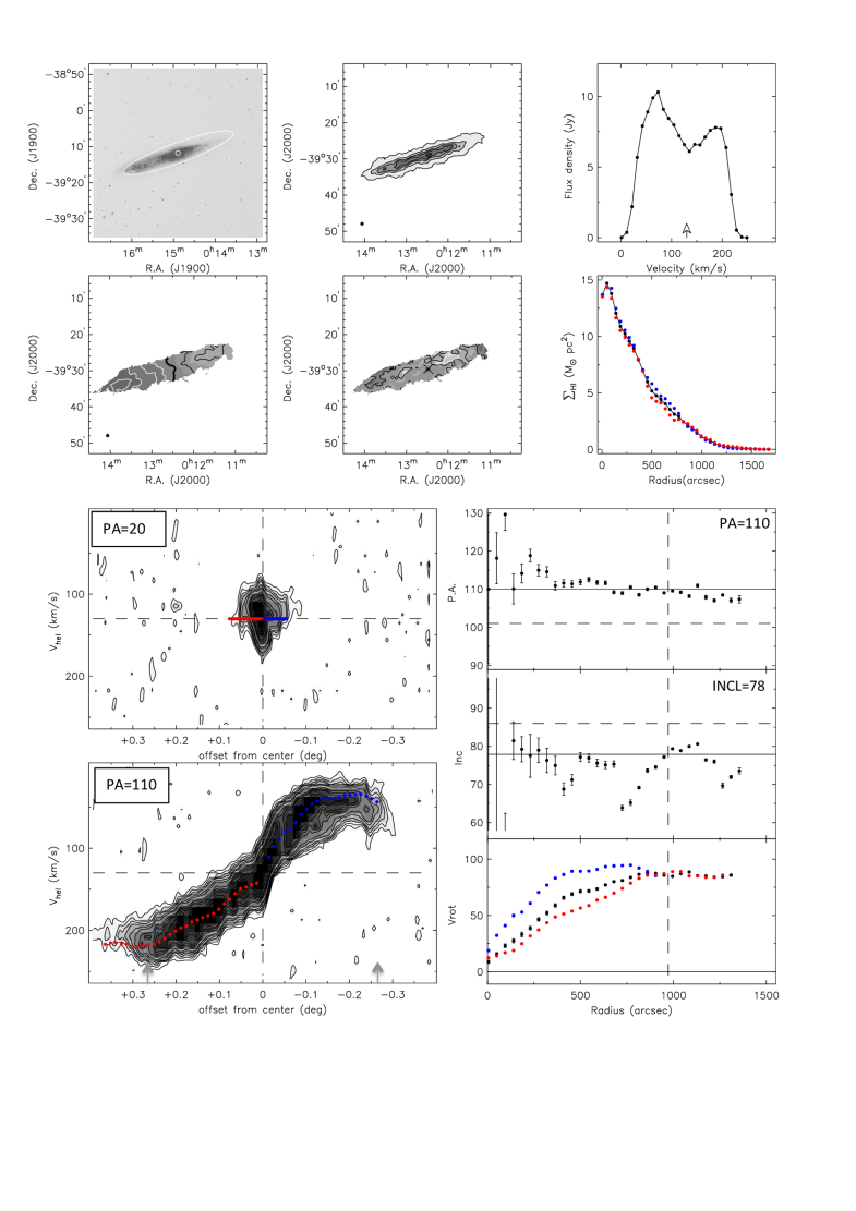
Figure 10: NGC 55 (VLA)

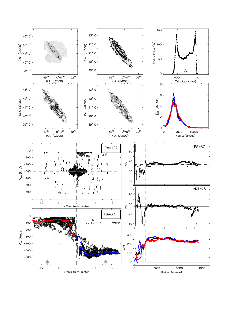
Figure 11: NGC 224 (WSRT)

Figure 12: NGC 247 (VLA)

Figure 13: NGC 253 (ATCA)

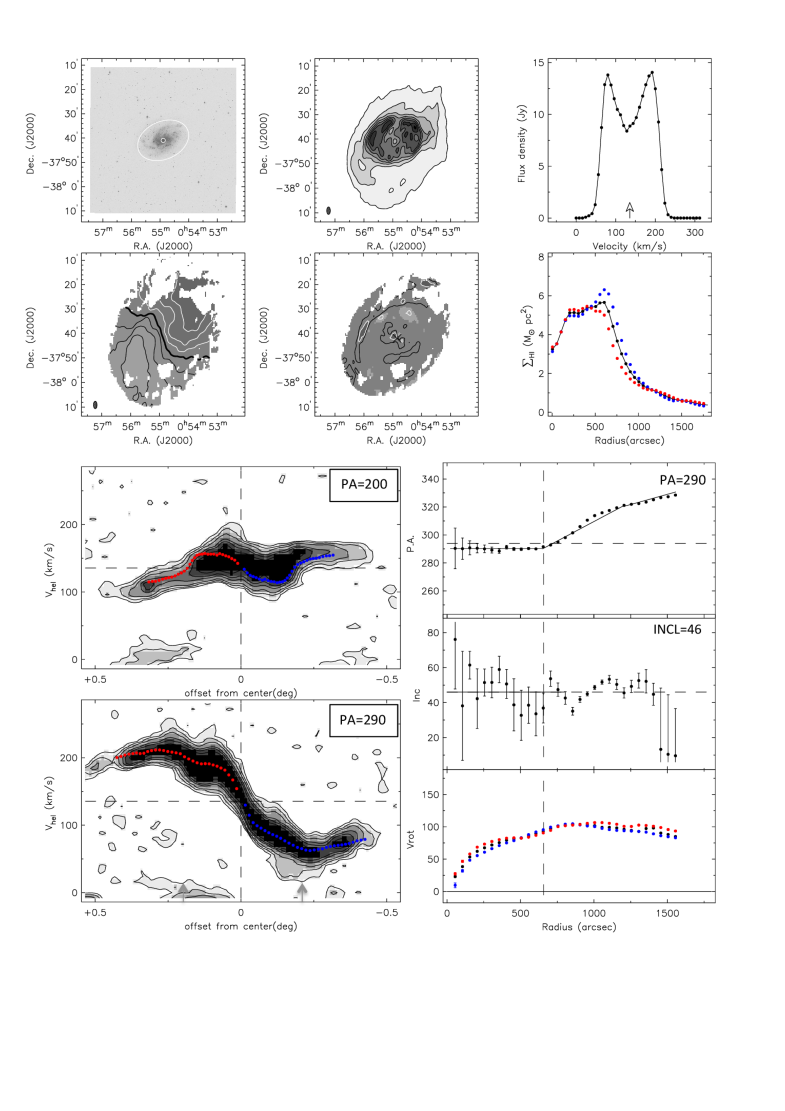
Figure 14: NGC 300 (ATCA)

Figure 15: NGC 925 (VLA)

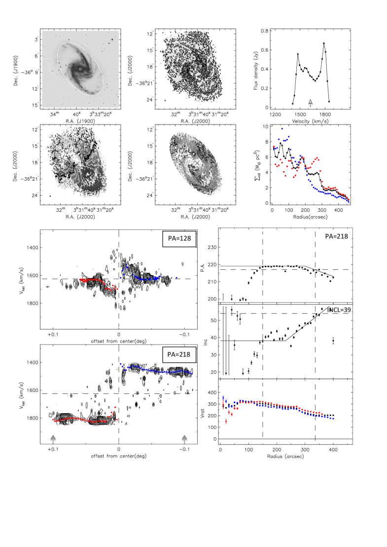
Figure 16: NGC 1365 (VLA)

Figure 17: NGC 2366 (VLA)

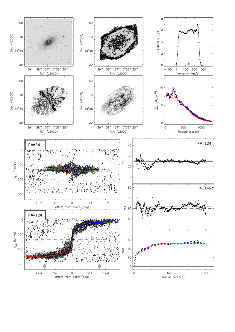
Figure 18: NGC 2403 (VLA)

Figure 19: NGC 2541 (WSRT)

Figure 20: NGC 2841 (VLA)

Figure 21: NGC 2976 (VLA)

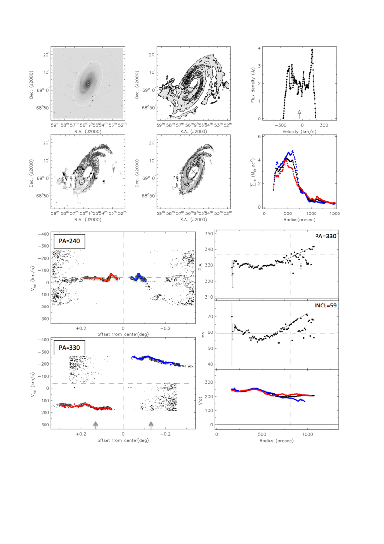
Figure 22: NGC 3031 (VLA)

Figure 23: NGC 3109 (VLA)

Figure 24: NGC 3198 (VLA)

Figure 25: IC 2574 (VLA)

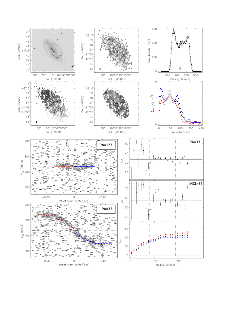
Figure 26: NGC 3319 (WSRT)

Figure 27: NGC 3351 (VLA)

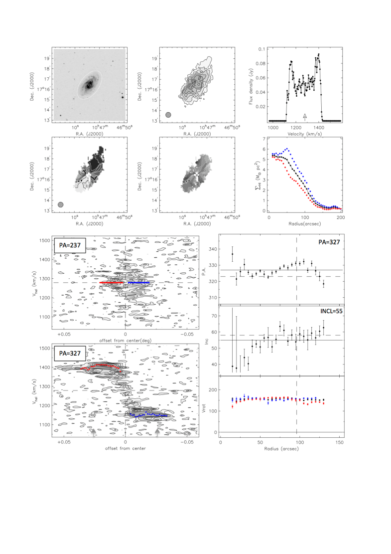
Figure 28: NGC 3370 (GMRT)

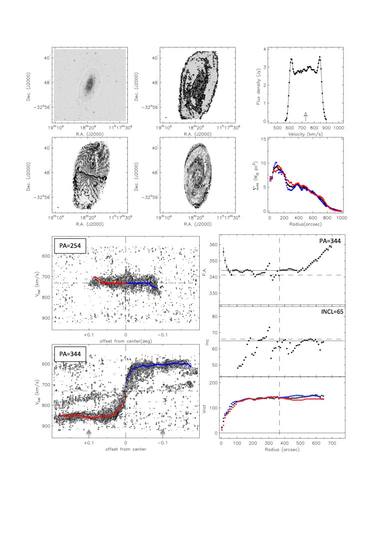
Figure 29: NGC 3621 (VLA)

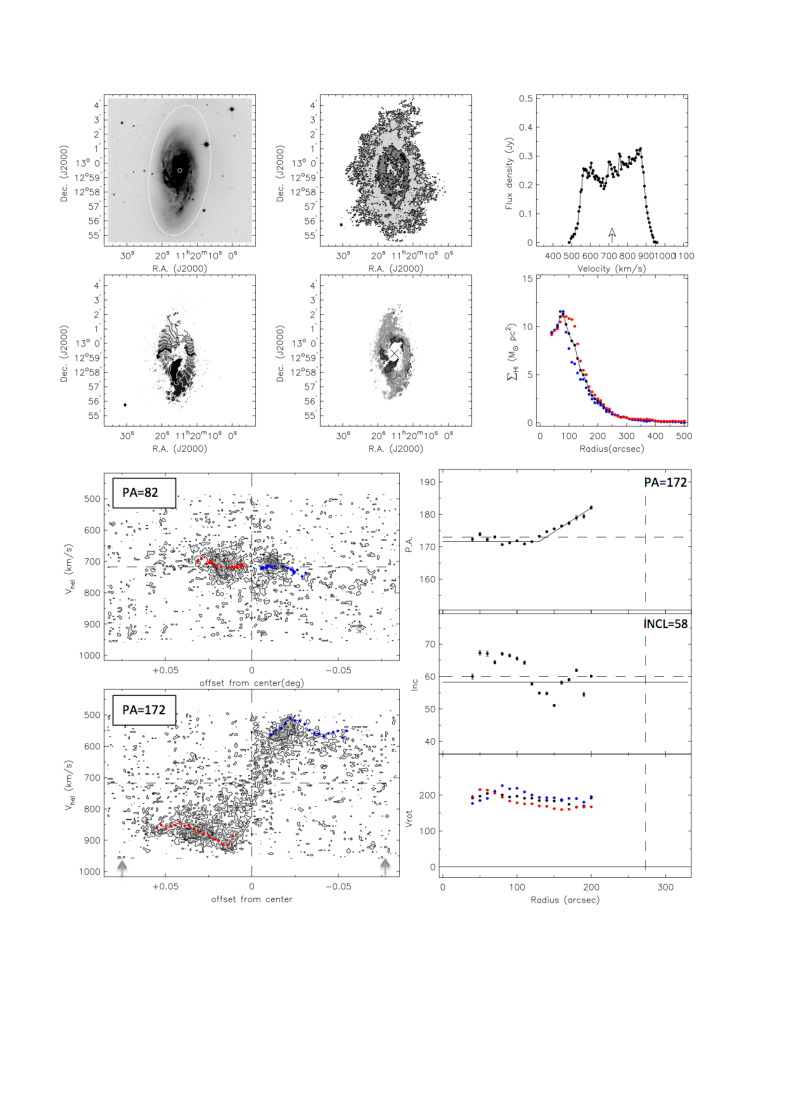
Figure 30: NGC 3627 (VLA)

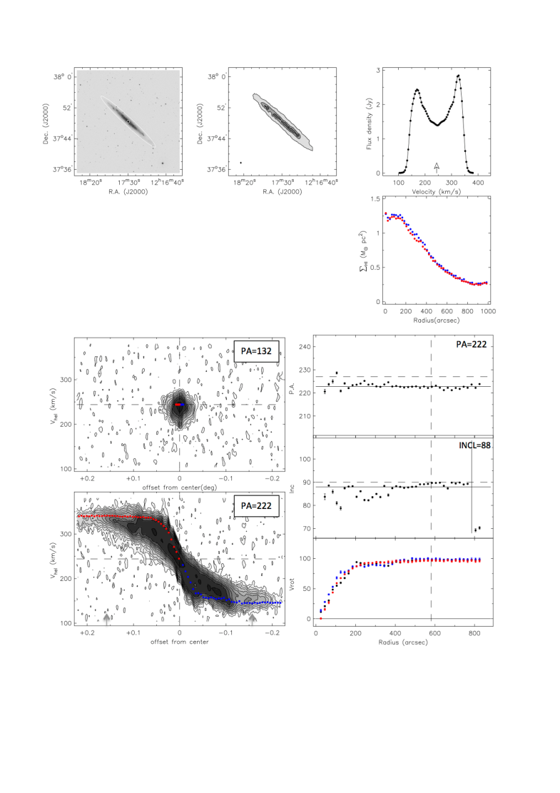
Figure 31: NGC 4244 (WSRT)

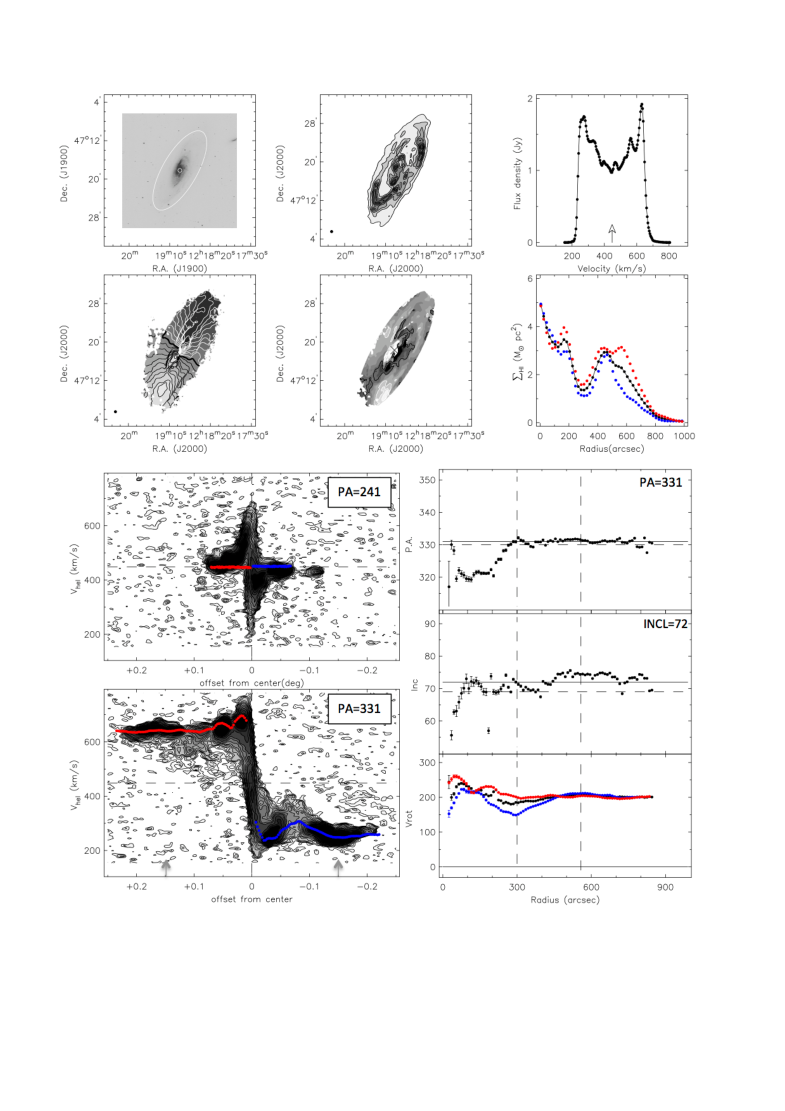
Figure 32: NGC 4258 (WSRT)

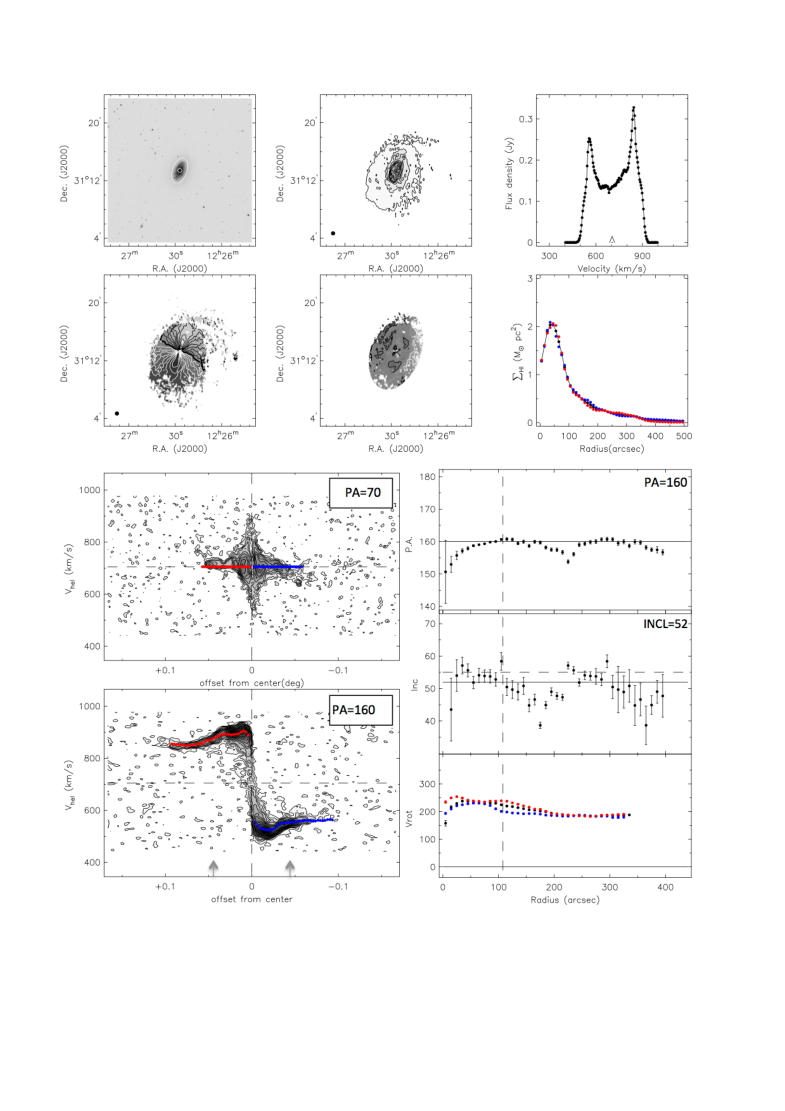
Figure 33: NGC 4414 (WSRT)

.pdf

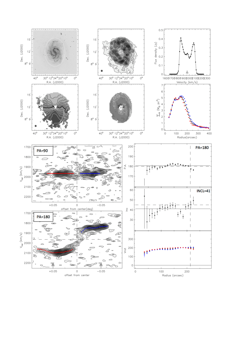
Figure 34: NGC 4535 (VLA)

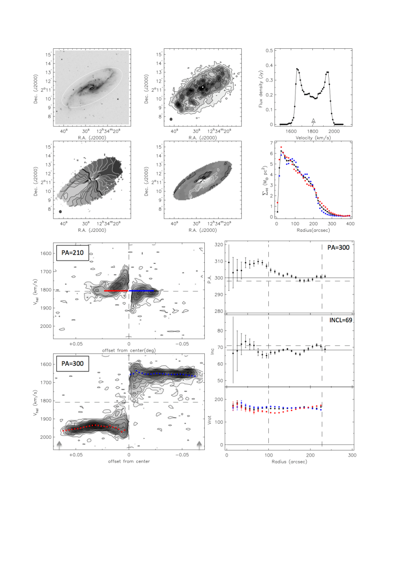
Figure 35: NGC 4536 (VLA)

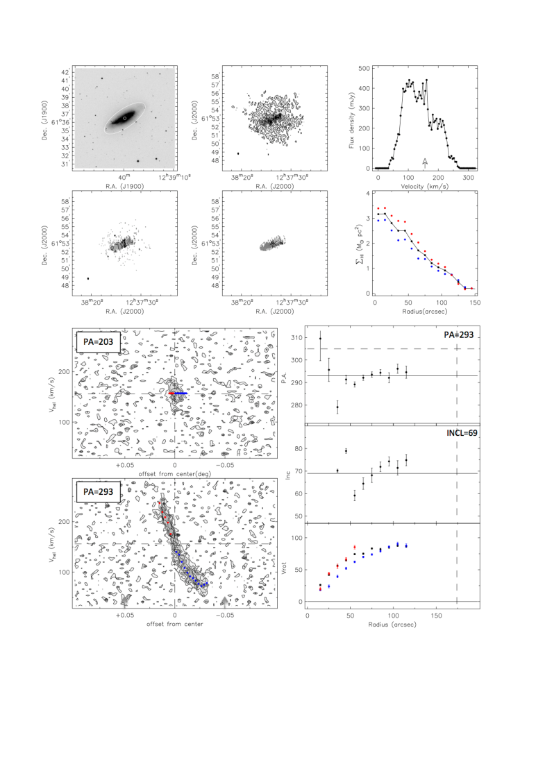
Figure 36: NGC 4605 (WSRT)

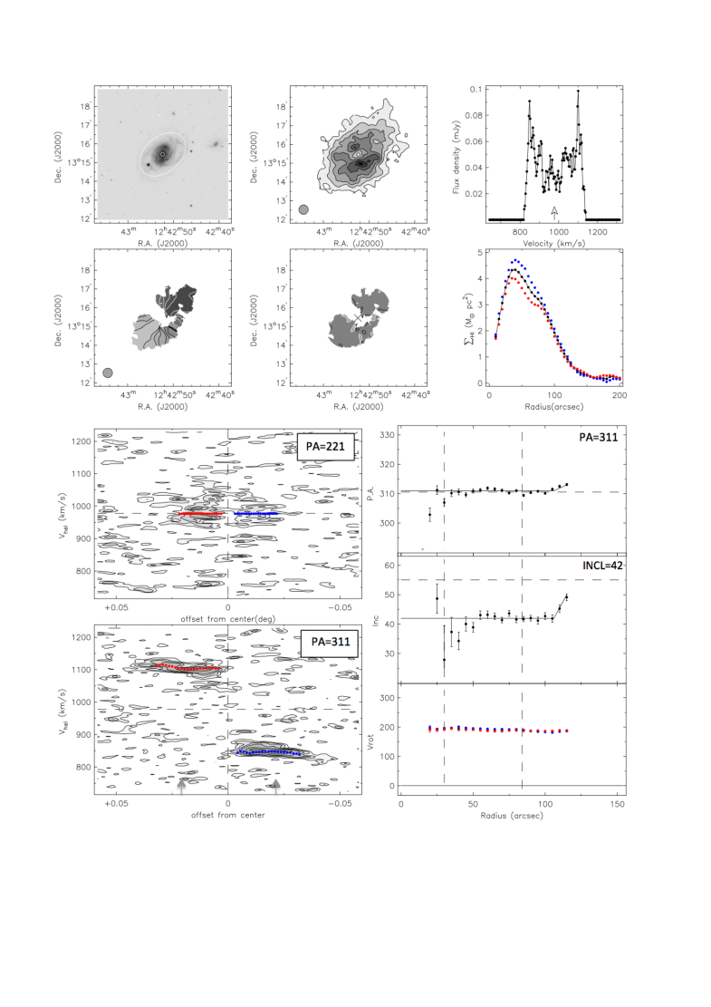
Figure 37: NGC 4639 (GMRT)

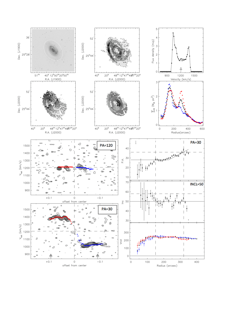
Figure 38: NGC 4725 (WSRT)

Figure 39: NGC 5584 (GMRT)

Figure 40: NGC 7331 (VLA)

Figure 41: NGC 7793 (VLA)

References

- Aaronson et al. (1979) Aaronson, M., Huchra, J., & Mould, J. 1979, ApJ, 229, 1
- Aaronson et al. (1980) Aaronson, M., Mould, J., & Huchra, J. 1980, ApJ, 237, 655
- Begeman (1989) Begeman, K. G. 1989, A&A, 223, 47
- Begeman (1987) Begeman, K. G. 1987, Ph.D. Thesis, University of Groningen, The Netherlands
- Bernstein et al. (1994) Bernstein, G. M., Guhathakurta, P., Raychaudhury, S., et al. 1994, AJ, 107, 1962
- Bosma (1978) Bosma, A. 1978, Ph.D. Thesis, University of Groningen, The Netherlands
- Bosma (1981) Bosma, A. 1981, AJ, 86, 1825
- Bottinelli et al. (1983) Bottinelli, L., Gouguenheim, L., Paturel, G., & de Vaucouleurs, G. 1983, A&A, 118, 4
- Braun et al. (2009) Braun, R., Thilker, D. A., Walterbos, R. A. M., & Corbelli, E. 2009, ApJ, 695, 937
- Broeils (1992) Broeils, A. H. 1992, Ph.D. Thesis,
- Broeils & van Woerden (1994) Broeils, A. H., & van Woerden, H. 1994, A&AS, 107, 129
- Casertano & van Gorkom (1991) Casertano, S., & van Gorkom, J. H. 1991, AJ, 101, 1231
- Carignan & Puche (1990) Carignan, C., & Puche, D. 1990, AJ, 100, 641
- Carignan & Puche (1990) Carignan, C., & Puche, D. 1990, AJ, 100, 394
- Carignan et al. (2013) Carignan, C., Frank, B. S., Hess, K. M., et al. 2013, AJ, 146, 48
- Chung et al. (2009) Chung, A., van Gorkom, J. H., Kenney, J. D. P., Crowl, H., & Vollmer, B. 2009, AJ, 138, 1741
- Corbelli et al. (2010) Corbelli, E., Lorenzoni, S., Walterbos, R., Braun, R., & Thilker, D. 2010, A&A, 511, A89
- Courtois et al. (2009) Courtois, H. M., Tully, R. B., Fisher, J. R., et al. 2009, AJ, 138, 1938
- Courtois et al. (2011) Courtois, H. M., Tully, R. B., Makarov, D. I., et al. 2011, MNRAS, 414, 2005
- de Blok et al. (2008) de Blok, W. J. G., Walter, F., Brinks, E., et al. 2008, AJ, 136, 2648
- de Blok et al. (2014) de Blok, W. J. G., Józsa, G. I. G., Patterson, M., et al. 2014, A&A, 566, A80
- Freedman et al. (2001) Freedman, W. L., Madore, B. F., Gibson, B. K., et al. 2001, ApJ, 553, 47
- Greisen (2003) Greisen, E. W. 2003, Information Handling in Astronomy - Historical Vistas, 285, 109
- Haynes et al. (2011) Haynes, M. P., Giovanelli, R., Martin, A. M., et al. 2011, AJ, 142, 170
- Heald et al. (2011) Heald, G., Józsa, G., Serra, P., et al. 2011, A&A, 526, A118
- Jörsäter & van Moorsel (1996) Jörsäter, S., & van Moorsel, C. A. 1996, IAU Colloq. 157: Barred Galaxies, 91, 168
- Koribalski et al. (2004) Koribalski, B. S., Staveley-Smith, L., Kilborn, V. A., et al. 2004, AJ, 128, 16
- Koribalski (2010) Koribalski, B. S. 2010, Galaxies in Isolation: Exploring Nature Versus Nurture, 421, 137
- Marinacci et al. (2014) Marinacci, F., Pakmor, R., & Springel, V. 2014, MNRAS, 437, 1750
- Martinsson (2011) Martinsson, T. P. K. 2011, Ph.D. Thesis, University of Groningen, The Netherlands
- McGaugh (2012) McGaugh, S. S. 2012, AJ, 143, 40
- Moore & Gottesman (1998) Moore, E. M., & Gottesman, S. T. 1998, MNRAS, 294, 353
- Navarro & Steinmetz (2000) Navarro, J. F., & Steinmetz, M. 2000, ApJ, 538, 477
- Noordermeer (2006) Noordermeer, E. 2006, Ph.D. Thesis,
- Oh et al. (2008) Oh, S.-H., de Blok, W. J. G., Walter, F., Brinks, E., & Kennicutt, R. C., Jr. 2008, AJ, 136, 2761
- Ott et al. (2012) Ott, J., Stilp, A. M., Warren, S. R., et al. 2012, AJ, 144, 123
- Pisano et al. (1998) Pisano, D. J., Wilcots, E. M., & Elmegreen, B. G. 1998, AJ, 115, 975
- Puche et al. (1990) Puche, D., Carignan, C., & Bosma, A. 1990, AJ, 100, 1468
- Puche et al. (1991) Puche, D., Carignan, C., & Wainscoat, R. J. 1991, AJ, 101, 447
- Puche et al. (1991) Puche, D., Carignan, C., & van Gorkom, J. H. 1991, AJ, 101, 456
- Rhee & van Albada (1996) Rhee, M.-H., & van Albada, T. S. 1996, A&AS, 115, 407
- Rizzi et al. (2007) Rizzi, L., Tully, R. B., Makarov, D., et al. 2007, ApJ, 661, 815
- Roberts & Haynes (1994) Roberts, M. S., & Haynes, M. 1994, European Southern Observatory Conference and Workshop Proceedings, 49, 197
- Sancisi & Allen (1979) Sancisi, R., & Allen, R. J. 1979, A&A, 74, 73
- Schaye et al. (2015) Schaye, J., Crain, R. A., Bower, R. G., et al. 2015, MNRAS, 446, 521
- Shetty et al. (2007) Shetty, R., Vogel, S. N., Ostriker, E. C., & Teuben, P. J. 2007, ApJ, 665, 1138
- Simon et al. (2003) Simon, J. D., Bolatto, A. D., Leroy, A., & Blitz, L. 2003, ApJ, 596, 957
- Simon et al. (2005) Simon, J. D., Bolatto, A. D., Leroy, A., Blitz, L., & Gates, E. L. 2005, ApJ, 621, 757
- Sorce et al. (2012) Sorce, J. G., Courtois, H. M., & Tully, R. B. 2012, AJ, 144, 133
- Sorce et al. (2013) Sorce, J. G., Courtois, H. M., Tully, R. B., et al. 2013, ApJ, 765, 94
- Springob et al. (2005) Springob, C. M., Haynes, M. P., & Giovanelli, R. 2005, ApJ, 621, 215
- Swaters et al. (2002) Swaters, R. A., van Albada, T. S., van der Hulst, J. M., & Sancisi, R. 2002, A&A, 390, 829
- Tully & Courtois (2012) Tully, R. B., & Courtois, H. M. 2012, ApJ, 749, 78
- Tully & Fisher (1977) Tully, R. B., & Fisher, J. R. 1977, A&A, 54, 661
- Tully et al. (1996) Tully, R. B., Verheijen, M. A. W., Pierce, M. J., Huang, J.-S., & Wainscoat, R. J. 1996, AJ, 112, 2471
- Tully et al. (1998) Tully, R. B., Pierce, M. J., Huang, J.-S., et al. 1998, AJ, 115, 2264
- Tully et al. (2009) Tully, R. B., Rizzi, L., Shaya, E. J., et al. 2009, AJ, 138, 323
- van Albada (1980) van Albada, G. D. 1980, A&A, 90, 123
- van Albada et al. (1985) van Albada, T. S., Bahcall, J. N., Begeman, K., & Sancisi, R. 1985, ApJ, 295, 305
- van der Hulst et al. (1992) van der Hulst, J. M., Terlouw, J. P., Begeman, K. G., Zwitser, W., & Roelfsema, P. R. 1992, Astronomical Data Analysis Software and Systems I, 25, 131
- van der Hulst et al. (2001) van der Hulst, J. M., van Albada, T. S., & Sancisi, R. 2001, Gas and Galaxy Evolution, 240, 451
- van der Marel & Franx (1993) van der Marel, R. P., & Franx, M. 1993, ApJ, 407, 525
- Verheijen (2001) Verheijen, M. A. W. 2001, ApJ, 563, 694
- Verheijen & Sancisi (2001) Verheijen, M. A. W., & Sancisi, R. 2001, A&A, 370, 765
- Visser (1980) Visser, H. C. D. 1980, A&A, 88, 149
- Vogelsberger et al. (2014) Vogelsberger, M., Genel, S., Springel, V., et al. 2014, MNRAS, 444, 1518
- Walter et al. (2008) Walter, F., Brinks, E., de Blok, W. J. G., et al. 2008, AJ, 136, 2563
- Weiner et al. (2001) Weiner, B. J., Sellwood, J. A., & Williams, T. B. 2001, ApJ, 546, 931
- Werner et al. (2004) Werner, M. W., Roellig, T. L., Low, F. J., et al. 2004, ApJS, 154, 1
- Westmeier et al. (2013) Westmeier, T., Koribalski, B. S., & Braun, R. 2013, MNRAS, 434, 3511
- Westmeier et al. (2011) Westmeier, T., Braun, R., & Koribalski, B. S. 2011, MNRAS, 410, 2217
- Wevers et al. (1984) Wevers, B. M. H. R., Appleton, P. N., Davies, R. D., & Hart, L. 1984, A&A, 140, 125
- Wright et al. (2010) Wright, E. L., Eisenhardt, P. R. M., Mainzer, A. K., et al. 2010, AJ, 140, 1868
- Zánmar Sánchez et al. (2008) Zánmar Sánchez, R., Sellwood, J. A., Weiner, B. J., & Williams, T. B. 2008, ApJ, 674, 797
- Zaritsky et al. (2014) Zaritsky, D., Courtois, H., Muñoz-Mateos, J.-C., et al. 2014, AJ, 147, 134
- Zschaechner et al. (2011) Zschaechner, L. K., Rand, R. J., Heald, G. H., Gentile, G., & Kamphuis, P. 2011, ApJ, 740, 35