Harmonic oscillators at resonance, perturbed by a non-linear friction force

Abstract

This note is an addendum to the results of A.C. Lazer and P.O. Frederickson [1], and A.C. Lazer [4] on periodic oscillations, with linear part at resonance. We show that a small modification of the argument in [4] provides a more general result. It turns out that things are different for the corresponding Dirichlet boundary value problem.

Key words: Resonance, existence of periodic solutions.

AMS subject classification: 34C25, 34C15, 34B15.

1 Introduction

We are interested in the existence of $2\pi$ periodic solutions to the problem ($x=x(t)$)

(1.1) $$x^{\prime\prime}+f(x)x^{\prime}+n^{2}x=e(t)\,.$$

Here $e(t)\in C(R)$ satisfies $e(t+2\pi)=e(t)$ for all $t$, $f(u)\in C(R)$, $n\geq 1$ is an integer. The linear part, $x^{\prime\prime}+n^{2}x=e(t)$, is at resonance, with the null space spanned by $\cos nt$ and $\sin nt$. Define $F(x)=\int_{0}^{x}f(t)\,dt$. We assume that the finite limits $F(\infty)$ and $F(-\infty)$ exist, and

(1.2) $$F(-\infty)<F(x)<F(\infty)\;\;\;\;\mbox{for all $x$}\,.$$

Define

$$A_{n}=\int_{0}^{2\pi}e(t)\cos nt\,dt,\;\;B_{n}=\int_{0}^{2\pi}e(t)\sin nt\,dt\,.$$

The following theorem was proved in case $n=1$ by A.C. Lazer [4], based on P.O. Frederickson and A.C. Lazer [1]. The paper [1] was the precursor to the classical works of E.M. Landesman and A.C. Lazer [3], and A.C. Lazer and D.E. Leach [3].

Theorem 1.1

The condition

(1.3) $$\sqrt{A_{n}^{2}+B_{n}^{2}}<2n\left(F(\infty)-F(-\infty)\right)$$

is necessary and sufficient for the existence of $2\pi$ periodic solution of (1.1).

We provide a proof for all $n$, by modifying the argument in [4].

Remarkably, things are different for the corresponding Dirichlet boundary value problem, for which we derive a necessary condition for the existence of solutions, but show by a numerical computation that this condition is not sufficient. Observe that the condition (1.3) depends on $n$, unlike the condition in A.C. Lazer and D.E. Leach [3].

2 The proof

The following elementary lemmas are easy to prove.

Lemma 2.1

Consider a function $\cos(nt-\varphi)$, with an integer $n$ and any real $\varphi$. Denote $P=\{t\in(0,2\pi)\,|\,\cos(nt-\varphi)>0\}$ and $N=\{t\in(0,2\pi)\,|\,\cos(nt-\varphi)<0\}$. Then

$$\int_{P}\cos(nt-\varphi)\,dt=2,\;\;\;\;\int_{N}\cos(nt-\varphi)\,dt=-2\,.$$

Lemma 2.2

Consider a function $\sin(nt-\varphi)$, with an integer $n$ and any real $\varphi$. Denote $P_{1}=\{t\in(0,2\pi)\,|\,\sin(nt-\varphi)>0\}$ and $N_{1}=\{t\in(0,2\pi)\,|\,\sin(nt-\varphi)<0\}$. Then

$$\int_{P_{1}}\sin(nt-\varphi)\,dt=2,\;\;\;\;\int_{N_{1}}\sin(nt-\varphi)\,dt=-2\,.$$

Proof of the Theorem 1.1:   1. Necessity. Given arbitrary numbers $a$ and $b$, we can find a $\delta\in[0,2\pi)$, so that

$$a\cos nt+b\sin nt=\sqrt{a^{2}+b^{2}}\cos(nt-\delta)\,.$$

($\cos\delta=\frac{a}{\sqrt{a^{2}+b^{2}}}$, $\sin\delta=\frac{b}{\sqrt{a^{2}+b^{2}}}$.) We multiply (1.1) by $a\cos nt$, then by $b\sin nt$, integrate and add the results

(2.1) $$I\equiv\int_{0}^{2\pi}F(x(t))^{\prime}\cos(nt-\delta)\,dt=\frac{aA_{n}+bB_{n}}{\sqrt{a^{2}+b^{2}}}\,.$$

Using that $x(t)$ is a $2\pi$ periodic solution, and Lemma 2.2, we have

$$I=n\int_{0}^{2\pi}F(x(t))\sin(nt-\delta)\,dt=n\int_{P_{1}}+n\int_{N_{1}}<2n\left(F(\infty)-F(-\infty)\right)\,.$$

Similarly,

$$I>-2n\left(F(\infty)-F(-\infty)\right)\,,$$

and so

$$|I|<2n\left(F(\infty)-F(-\infty)\right)\,.$$

On the right in (2.1) we have the scalar product of the vector $(A_{n},B_{n})$ and an arbitrary unit vector. The condition (1.3) follows.

2. Sufficiency. We write our equation $\left(x^{\prime}+F(x)\right)^{\prime}+n^{2}x=e(t)$ in the system form

(2.2) $$x^{\prime}=-F(x)+y$$

$$y^{\prime}=-n^{2}x+e(t)\,.$$

Setting $x=\frac{1}{n}X$, $y=Y$, we get

(2.3) $$X^{\prime}=-nF(\frac{1}{n}X)+nY$$

$$Y^{\prime}=-nX+e(t)\,.$$

Let $r(t)=\sqrt{X^{2}(t)+Y^{2}(t)}$. Then

(2.4) $$r^{\prime}(t)=\frac{XX^{\prime}+YY^{\prime}}{r(t)}=\frac{-nXF(\frac{1}{n}X)+e(t)Y}{r(t)}\,.$$

We see that if $r(t)$ is large, $r^{\prime}(t)$ is bounded. It follows that there exists $r_{0}>0$, so that if $|r(0)|>r_{0}$, then $r(t)>0$ for all $t\in[0,2\pi]$, thus avoiding a singularity in (2.4). Switching to the polar coordinates $X(t)=r(t)\cos\theta(t)$ and $Y(t)=r(t)\sin\theta(t)$, (2.4) becomes

(2.5) $$r^{\prime}(t)=-nF\left(\frac{1}{n}r(t)\cos\theta(t)\right)\cos\theta(t)+e(t)\sin\theta(t)\,.$$

We have $\theta(t)=\tan^{-1}\frac{Y(t)}{X(t)}$, and

$$\theta^{\prime}(t)=\frac{-YX^{\prime}+XY^{\prime}}{X^{2}+Y^{2}}=\frac{nYF(\frac{1}{n}X)-nX^{2}-nY^{2}+e(t)X}{X^{2}+Y^{2}}\,.$$

In polar coordinates

(2.6) $$\theta^{\prime}(t)=-n+\frac{nF\left(\frac{1}{n}r(t)\cos\theta(t)\right)\sin\theta(t)}{r(t)}+\frac{e(t)\cos\theta(t)}{r(t)}\,.$$

We denote by $r(t,c,\varphi)$ and $\theta(t,c,\varphi)$ the solution of the system (2.5), (2.6) satisfying the initial conditions $r(0,c,\varphi)=c$ and $\theta(0,c,\varphi)=\varphi$.

From (2.5)

(2.7) $$r(t,c,\varphi)=c+O(1),\;\;\mbox{as $c\rightarrow\infty$}$$

uniformly in $t,\varphi\in[0,2\pi]$. Then from (2.6)

(2.8) $$\theta(t,c,\varphi)=-nt+\varphi+o(1),\;\;\mbox{as $c\rightarrow\infty$}$$

uniformly in $t,\varphi\in[0,2\pi]$. Integrating (2.5)

$$r(2\pi,c,\varphi)-r(0,c,\varphi)=\int_{0}^{2\pi}\left[-nF\left(\frac{1}{n}r(t)\cos\theta(t)\right)\cos\theta(t)+e(t)\sin\theta(t)\right]\,dt\,.$$

We have $\cos\theta(t)=\cos(nt-\varphi)+o(1)$, and $\sin\theta(t)=\sin(-nt+\varphi)+o(1)$, as $c\rightarrow\infty$. Then, in view of (2.7) and Lemma 2.1, the integral on the right gets arbitrarily close to

$$-2n\left(F(\infty)-F(-\infty)\right)+\int_{0}^{2\pi}e(t)\sin(-nt+\varphi)\,dt\,,$$

for $c$ sufficiently large. Since

$$\int_{0}^{2\pi}e(t)\sin(-nt+\varphi)\,dt=A_{n}\sin\varphi-B_{n}\cos\varphi<\sqrt{A_{n}^{2}+B_{n}^{2}}\,,$$

it follows by our condition (1.3) that

$$r(2\pi,c,\varphi)<r(0,c,\varphi)=c\,,$$

for $c$ sufficiently large, uniformly in $\varphi\in[0,2\pi]$, say for $c>c_{1}$. Denote $c_{2}=\max_{c\leq c_{1},\,\varphi\in[0,2\pi]}r(2\pi,c,\varphi)$, and $c_{3}=\max(c_{1},c_{2})$. (Here $r(2\pi,c,\varphi)$ is computed by using (2.2).) Then $r(2\pi,c,\varphi)\leq c_{3}$, provided that $c\leq c_{3}$. The map $(c,\varphi)\rightarrow\left(r(2\pi,c,\varphi),\theta(2\pi,c,\varphi)\right)$ is a continuous map of the ball $c\leq c_{3}$ into itself. By Brouwer’s fixed point theorem it has a fixed point, giving us a $2\pi$ periodic solution. $\diamondsuit$

3 A boundary value problem

Consider the Dirichlet problem

(3.1) $$x^{\prime\prime}-F(x)^{\prime}+x=e(t),\;\;0<t<\pi,\;\;x(0)=x(\pi)=0\,.$$

Assume that $F(x)$ satisfies (1.2), $e(t)\in C[0,\pi]$. The linear part has a kernel spanned by $\sin t$. Denote $A=\int_{0}^{\pi}e(t)\sin t\,dt$. Then from (3.1)

$$A=\int_{0}^{\pi}F(x(t))\cos t\,dt<F(\infty)\int_{0}^{\pi/2}\cos t\,dt+F(-\infty)\int_{\pi/2}^{\pi}\cos t\,dt$$

$$=F(\infty)-F(-\infty)\,.$$

Similarly,

$$A>F(-\infty)-F(\infty)\,.$$

We conclude that

(3.2) $$|A|<F(\infty)-F(-\infty)$$

is a necessary condition for the existence of solutions.

It is natural to ask if the condition (3.2) is sufficient for the existence of solutions. The following numerical computations indicate that the answer is No.

Example We have solved the problem

(3.3) $$x^{\prime\prime}-F(x)^{\prime}+x=A\sin t+\sin 2t,\;\;0<t<\pi,\;\;x(0)=x(\pi)=0\,,$$

with $F(x)=\frac{x}{\sqrt{x^{2}+1}}$. Here $F(\pm\infty)=\pm 1$, and so the necessary condition for the existence of solutions is $\displaystyle|A|<2$. Writing the solution as $x(t)=\xi\sin t+X(t)$, with $\int_{0}^{\pi}X(t)\sin t\,dt=0$, for each value of $\xi$ we compute the value of $A$ for which the problem (3.3) has a solution with the first harmonic equal to $\xi$, and that solution $x(t)$, see P. Korman [2] for more details. (I.e., we compute the solution curve $(A,x(t))(\xi)$.) In Figure $1$ we draw the curve $A=A(\xi)$. It suggests that there is an $A_{0}\approx-0.3$ so that the problem (3.3) has exactly two solutions for $A\in(A_{0},0)$, exactly one solution for $A=(A_{0},0)$, and no solutions for all other values of $A$. The necessary condition $\displaystyle|A|<2$ is definitely not sufficient!

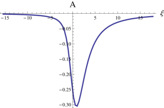
Figure 1: Solution curve for the problem (3.1)

References

- [1] P.O. Frederickson and A.C. Lazer, Necessary and sufficient damping in a second-order oscillator, J. Differential Equations 5, 262-270 (1969).
- [2] P. Korman, Global solution curves for boundary value problems, with linear part at resonance, Nonlinear Anal. 71, no. 7-8, 2456-2467 (2009).
- [3] E.M. Landesman and A.C. Lazer, Nonlinear perturbations of linear elliptic boundary value problems at resonance, J. Math. Mech. 19, 609-623 (1970).
- [4] A.C. Lazer, A second look at the first result of Landesman-Lazer type. Proceedings of the Conference on Nonlinear Differential Equations (Coral Gables, FL, 1999), 113-119 (electronic), Electron. J. Differ. Equ. Conf., 5, Southwest Texas State Univ., San Marcos, TX, (2000).
- [5] A.C. Lazer and D.E. Leach, Bounded perturbations of forced harmonic oscillators at resonance, Ann. Mat. Pura Appl. 82 (4), 49-68 (1969).