Hydrodynamical model atmospheres: Their impact on stellar spectroscopy and asteroseismology of late-type stars

Abstract

Hydrodynamical, i.e. multi-dimensional and time-dependent, model atmospheres of late-type stars have reached a high level of realism. They are commonly applied in high-fidelity work on stellar abundances but also allow the study of processes that are not modelled in standard, one-dimensional hydrostatic model atmospheres. Here, we discuss two observational aspects that emerge from such processes, the photometric granulation background and the spectroscopic microturbulence. We use CO5BOLD hydrodynamical model atmospheres to characterize the total granular brightness fluctuations and characteristic time scale for FGK stars. Emphasis is put on the diagnostic potential of the granulation background for constraining the fundamental atmospheric parameters. We find a clear metallicity dependence of the granulation background. The comparison between the model predictions and available observational constraints at solar metallicity shows significant differences, that need further clarification. Concerning microturbulence, we report on the derivation of a theoretical calibration based on CO5BOLD models, which shows good correspondence with the measurements for stars in the Hyades. We emphasize the importance of a consistent procedure when determining the microturbulence, and point to limitations of the commonly applied description of microturbulence in hydrostatic model atmospheres.

1 Introduction

The structure of late-type stellar atmospheres is mainly shaped by two processes: radiation and convection. The standard modelling approach of these atmospheres tries to capture the properties of the stellar radiation field in great detail while the gas-dynamical aspects are simplified by assuming one-dimensional (1D), plane-parallel or spherical symmetry. Mixing-length theory is employed to model the energy transport by convection. In contrast, hydrodynamical, 3D model atmospheres put emphasis on the representation of convection, trying to capture the complex geometry and time-dependence of the gas flows. This comes at the expense of a less detailed treatment of the radiation field in comparison to 1D models. Nevertheless, the treatment of radiation is sufficiently accurate to derive the atmospheric structure with a high degree of realism, e.g., demonstrated by the exquisite reproduction of the solar center-to-limb variation of the line-blanketed intensity at different wavelengths (e.g., Koesterke et al. 2008; Ludwig et al. 2010).

The main application of model atmospheres is the analysis of stellar (electromagnetic) spectra, i.e., the derivation of a star’s atmospheric parameters and its chemical composition. To this end the precise knowledge of the thermal structure of the stellar atmosphere is essential. And indeed, differences in the thermal structure between 1D and 3D models cause differences in the derived parameters and composition. Applications of the 3D model atmospheres documented in the literature mainly revolve around abundance issues (see Amarsi et al. 2015; Caffau et al. 2015; Dobrovolskas et al. 2015; Scott et al. 2015, as recent examples), and are commonly rooted in differences between the thermal structure of 1D and 3D models.

Besides predicting changes in the thermal properties, 3D models provide information on the flow dynamics taking place in a stellar atmosphere. Knowledge of the velocity field allows one to eliminate the classical free parameters of micro- and macro turbulence in spectral analysis. Moreover, pressure fluctuations associated with the non-stationary flow are believed to be the exciting agent of solar-like oscillations in late-type stars which establishes a link to asteroseismology (Nordlund & Stein 2001; Samadi et al. 2007, 2013a).

In this contribution we intend to discuss ongoing projects in the field of spectroscopy and asteroseismology besides the main application of 3D models in abundance work. They are related to i) the diagnostic potential of the so-called granulation background; and ii) microturbulence calibration with 3D models and related insights concerning the deficiencies of classical 1D model atmospheres. The reader should be aware that both examples are work in progress, so not all issues are fully worked out.

2 Granulation background across the Hertzsprung-Russell diagram

2.1 The sample of 3D model atmospheres

Figure 1 depicts the sample of so-called “local-box” 3D models which we used to investigate the granulation background across the Hertzsprung-Russell diagram (HRD). The models were taken from the CIFIST 3D model atmosphere grid (Ludwig et al. 2009a) calculated with the radiation-hydrodynamics code CO⁵BOLD (Freytag et al. 2012), however continued in time to obtain extra long time series. Ten models assume solar metallicity, nine models are very metal-poor at $\left[\mathrm{M/H}\right]=-2$. The strong metallicity contrast was chosen to obtain a clear signal related to metallicity effects. The models cover the main-sequence in the FGK temperature range and the lower red giant branch, the primary region where CoRoT and Kepler targets are located.

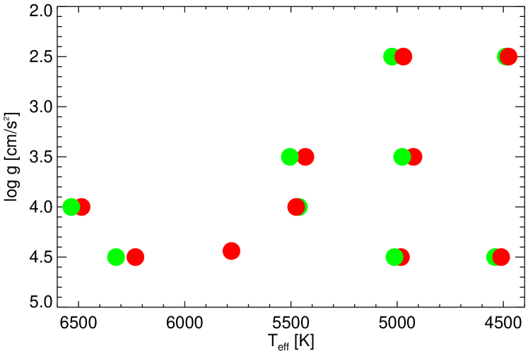
Figure 1: The investigated 19 3D models in the $T_{\mathrm{eff}}$-$\log g$ plane. Ten are of solar metallicity (red cirles), nine of sub-solar metallicity $\left[\mathrm{M/H}\right]=-2$ (green circles).

2.2 From local box models to global brightness fluctuations

A 3D model provides a realization of the convective flows in a representative volume at the stellar surface. This includes detailed information on the emergent intensity as a function of surface position, frequency, and direction. Ludwig (2006) laid out a procedure for scaling the radiative output of a local model to disk-integrated light. Conceptually, the stellar surface is considered to be tiled by a (potentially great) number of model “tiles” or “patches”. Only the horizontally averaged, frequency-integrated emergent intensity needs to be considered so that all information taken from a model is a time series of the bolometric intensity $I_{\mathrm{bol}}$ at different limb-angle cosines $\mu_{i}$, i.e., $I_{\mathrm{bol}}(t,\mu_{i})$ where $t$ denotes time. The scaling assumes that the horizontal extent of a model patch is large enough that the emission of neighboring patches is not correlated. The emission of the ensemble of patches tiling the visible stellar hemisphere is an outcome of the incoherent action of all patches. This assumption is appropriate for the small-scale random granulation pattern but inadequate for oscillatory modes which are coherent on the global stellar scale. In 3D models acoustic oscillations take place as well, however, they manifest themselves as eigenmodes of the computational domain, and their amplitudes cannot be directly compared with observed modes.

One does not need to perform the tiling procedure explicitely. The relevant property of each model tile is its surface area fraction contributing to the total flux. For each parameter combination the simulations provide only a single time series of the emergent intensities. To generate other statistically independent realizations for other tiles the phases of the Fourier components of the simulated time series are shifted randomly and independently (see Ludwig 2006, for details).

The outcome of the scaling procedure is an estimate of the power spectrum of observable, global brightness fluctuations of a star related to granulation. An input parameter to the scaling that was not mentioned yet is the stellar radius $R$. $R$ is not a control parameter of a local 3D model nor a result of the calculation. It is an external piece of information, and needs to be provided by other consideration in the scaling procedure, e.g., by considering evolutionary stellar models. The total (frequency-integrated) granulation-related brightness fluctuations ${\sigma_{\mathrm{gran}}}$ scale inversely proportional to $R$. To avoid ambiguities and uncertainties stemming from the choice of $R$ we usually work with a scaled measure of the brightness fluctuations ${\tilde{\sigma}_{\mathrm{gran}}}$ defined as

$${\tilde{\sigma}_{\mathrm{gran}}}\equiv\frac{R}{\mathrm{R}_{\odot}}\,{\sigma_{\mathrm{gran}}}$$ (1)

where $\mathrm{R}_{\odot}$ denotes the solar radius. ${\tilde{\sigma}_{\mathrm{gran}}}$ can be calculated from the local box models alone.

The duration of a time series of 3D models is limited by the affordable computing time. In comparison to observational time series the simulated series are short, making the resulting power spectra noisy. To extract the granular signal from the calculated power spectrum and eliminate the contribution of oscillatory modes we fit a simple analytical model to the simulated spectrum of the form

$$\frac{dP}{d\nu}(\nu)=\frac{\tilde{\sigma}^{2}_{\mathrm{gran}}}{\nu_{\mathrm{gran}}}\exp\left(-\nu/\nu_{\mathrm{gran}}\right)+\mbox{sum of Lorentzians}\,.$$ (2)

$\nu_{\mathrm{gran}}$ is the characteristic granular frequency. A sum of Lorentzian-shaped peaks model the contribution of the (usually two or three) oscillatory modes present in the time series. As final result a 3D model provides a prediction of the scaled granular brightness fluctuations ${\tilde{\sigma}_{\mathrm{gran}}}$ and characteristic frequency $\nu_{\mathrm{gran}}$. We later use this to construct an “inverse” HRD of convective properties (see Sect. 2.3).

Figure 2 shows a synthetic power spectrum together with a fit according to Eq. (2). The high frequency part ($>6\mbox{\rm\,mHz}$) was not included in the fitting and should be ignored. The figure depicts the typical run of the granulation background signal in the power spectra. The frequencies of the (two) box modes roughly coincide with the mode frequencies expected in a star since the frequencies where modes are excited are governed by surface convection.

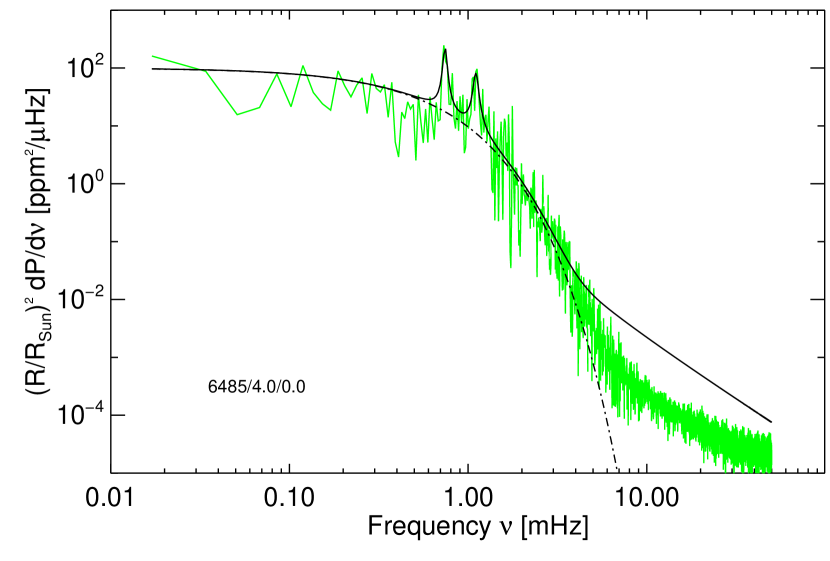
Figure 2: Example of a synthetic power spectrum for an F-dwarf model (green solid line), and fitted power spectra including (black solid line) and leaving-out (dashed-dotted line) p-modes. For display purposes the synthetic power spectrum was smoothed

2.3 “Inverse” Hertzsprung-Russell diagram of convective properties

Figure 3 depicts the derived ${\tilde{\sigma}_{\mathrm{gran}}}$ and $\nu_{\mathrm{gran}}$ in the HRD. Instead of plotting the values as function of $T_{\mathrm{eff}}$, $\log g$, and $\left[\mathrm{M/H}\right]$ we provide the inverse functions to emphasize the diagnostic potential of the granulation-related properties. Measurements of ${\sigma_{\mathrm{gran}}}$ and $\nu_{\mathrm{gran}}$ from observed time series, together with information on the stellar radius and metallicity allow us to constrain the fundamental atmospheric parameters $T_{\mathrm{eff}}$ and $\log g$. In Fig. 3 bilinear fits for both metallicities are shown separately. A simultaneous fit of both metallicity sets did not work satisfactorily, presumably due to the large jump in metallicity between them. The bilinear fits were performed in log-space corresponding to power laws in linear space commonly used in asteroseimic scaling relations. The fitting residuals indicate that there is perhaps structure beyond simple power laws, however, the estimated uncertainties of the model results (due to limited length of the time series) do not allow to make a definite statement.

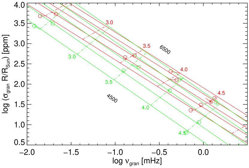
Figure 3: Scaled granular brightness fluctuations ${\tilde{\sigma}_{\mathrm{gran}}}=R/\mathrm{R}_{\odot}\,{\sigma_{\mathrm{gran}}}$ and characteristic granular frequencies $\nu_{\mathrm{gran}}$ of the 3D models. Red circles mark the location of models of solar metallicity, green circles of $\left[\mathrm{M/H}\right]=-2$. The lines depict bilinear fits to the data points labelled by (log) surface gravity (dashed-dotted lines), and effective temperature (solid lines) running from 4500 K to 6500 K in steps of 500 K. Short line segments attached to the data points depict the fitting residuals.

2.4 Discussion

The most robust result of our investigation is the about twice as high temperature sensitivity of the brightness fluctuations at $\left[\mathrm{M/H}\right]=-2$ in comparison to the sensitivity at solar metallicity (as indicated by the widths of the bands in Fig. 3). However, the magnitude of the sensitivity – at least at solar metallicity – is apparently not compatible with observations: Kallinger et al. (2014) observe a smaller T-sensitivity than predicted by Samadi et al. (2013b). Samadi and collaborators also use CIFIST 3D models for deriving the brightness fluctuations but applying a different methodology as we do here. Nevertheless, our T-sensitivities are compatible with the values derived by Samadi et al. so that we arrive at the same conclusion as Kallinger et al.. The reason for the discrepancy is presently unclear but further investigations are under way.

Bastien et al. (2013) and Cranmer et al. (2014) promote the so-called “8-hour flicker” as gravimeter in late-type stars. We filtered our simulated light curves similar to the procedure when measuring the 8-hour flicker, and compared the resulting brightness fluctuations with observational data presented by Cranmer et al. (2014). We applied a bolometric correction as given by Ballot et al. (2011) to the observed fluctuations. We find (not shown) a reasonable agreement in giants. However, in dwarfs the 3D models predict a weaker 8-hour flicker than observed. There are various factors that may play a role: The observational data still contains the oscillatory component enhancing the signal which is absent in the theoretical prediction. Moreover, stellar activity which is not included in out 3D models might enhance fluctuations. In contrast, granulation in hot (F-type) stars should suffer from magnetic suppression (Cranmer et al. 2014; Ludwig et al. 2009b) reducing the observed signal. Which effect dominates, or whether the cause lies in the mentioned aspects at all, is not clear yet. However, the 8-hour flicker is not very-well adapted to dwarfs since it measures only a small fraction of the underlying granular signal due to the rather long time scales the 8-hour signal puts emphasis on. Hence, we consider the discrepancy in the 8-hour flicker not particularly problematic.

All in all one is confronted with the situation that the correspondence between model prediction and observations is not satisfactory. We expect that a fully consistent analysis of observational and model data (e.g., applying the same granular background model) will lead to improvements. We do not think that a refined treatment of the radiative transfer will help since the bulk of the radiation emerges from the low photosphere which is already represented well. Beyond that, we think it becomes apparent that some physics is missing in the models where magnetic activity related effects are prime suspects here. It will be interesting to identify more clearly where in the HRD this is of importance.

3 Microturbulence issues

In 1D abundance analyses, the microturbulence $\xi_{\mathrm{micro}}$ is usually considered a “nuisance” parameter since it needs to be determined without being of primary interest. The microturbulence influences the strength of partly saturated lines and is interpreted as the effect of the small-scale photospheric velocity field that 1D models are not accounting for. Less evident, the microturbulence can also compensate offsets in the thermal structure between model and star. It is usually described by a depth-independent, isotropic Gaussian broadening of fixed width $\xi_{\mathrm{micro}}$, adjusted to make weak and strong lines provide the same abundance. At low spectral resolution or low signal-to-noise ratio – a typical situation encountered in large scale spectroscopic surveys – abundance analysis relies on strong lines. Strong lines are not optimal for abundance work but under the given circumstances the only available abundance indicators. If only strong lines are detectable, no measurement of $\xi_{\mathrm{micro}}$ is possible so that one is in need of an either empirical or theoretical calibration giving the microturbulence as function of effective temperature, surface gravity, and metallicity. 3D models predict atmospheric velocity fields, and can provide theoretical estimates. It is perhaps fair to say that the observational picture of the microturbulence is rather messy, in the sense that the existence of a tight correlation between $\xi_{\mathrm{micro}}$ and stellar spectral type seems not evident. In part, this may be related to commonly neglected processes when discussing the microturbulence like stellar rotation or activity. Another problematic aspect lies in the fact that the derived value of the microturbulence also depends on the set of lines selected for its determination.

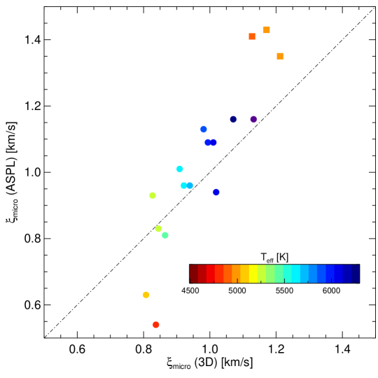
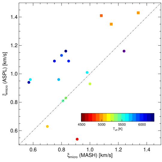
Figure 4: Top: Microturbulence of dwarfs (circles) and giants (squares) in the Hyades. Measurements based on Fe i lines taken from the “ASPL” list are plotted against the 3D predicted values. Color encodes stellar effective temperature. The dashed-dotted line indicates the one-to-one correspondence. Bottom: Comparison of the empirical microturbulence measurements based on, respectively, the “ASPL” and “MASH” iron line list.

3.1 Microturbulence from 3D models

3D models can provide reasonable predictions of the microturbulence necessary for 1D analysis work. Steffen et al. (2013) laid out different procedures of how to derive $\xi_{\mathrm{micro}}$ from 3D models. Dutra-Ferreira et al. (2015) give a recent example of applying a calibration of $\xi_{\mathrm{micro}}$ from 3D models. They studied dwarfs and giants in the Hyades using high-quality UVES and HARPS spectra. Besides using their calibration based on 3D models, they also determined the microturbulence in the classical spectroscopic way. For this purpose, they applied two different lists of iron lines, named “ASPL” and “MASH”. Figure 4 (top) shows the comparison between the 3D calibrated microturbulence and the empirical values obtained with the “ASPL” line list. For each star, the 3D microturbulence was obtained from the analytical expression by Dutra-Ferreira et al. (their Eq. 2) with the spectroscopic values of $T_{\mathrm{eff}}$ and $\log g$ given in their Table 6. Note that the 3D $\xi_{\mathrm{micro}}$ calibration is based on the same selection of “ASPL” lines as used for the classical spectroscopic microturbulence determination.

The correspondence is quite satisfactory for stars with $T_{\mathrm{eff}}$ above $5000$ K, where deviations are typically less than 0.1 km/s. For the two cool dwarfs, the microturbulence predicted by the 3D models seems significantly higher than inferred empirically, but we note that the measurement uncertainty is rather high for these objects, about 0.2 km/s. For the three giants, we find the opposite situation. Here the microturbulence predicted by the 3D models is too low. This may be attributed to an insufficient spatial resolution of the 3D simulations for the giants (see Steffen et al. 2013, for a discussion of the resolution dependence of $\xi_{\mathrm{micro}}$ derived from the 3D models).

Dutra-Ferreira et al. also derived the microturbulence of their target stars based on the MASH line list. Figure 4 (bottom) compares the resulting values between the two lists, emphasizing the point that the derived microturbulence depends on the chosen line list (systematic offset, sizable scatter). One should appreciate that ambiguities in the microturbulence determination translate into systematic uncertainties in atmospheric parameters and chemical abundances.

3.2 Center-to-limb trouble

It has been known for a long time from the analysis of spectra taken at different positions across the solar disk that microturbulence is a function of the limb angle $\theta$ ($\mu$ = $\cos\theta$ = $1$ at disk center, $\mu$ = $0$ at the limb). According to Holweger et al. (1978), $\xi_{\mathrm{micro}}$ $\approx 1.0$  km/s at disk center, while $\xi_{\mathrm{micro}}$ $\approx 1.6$  km/s near the solar limb. Our 3D hydrodynamical solar CO⁵BOLD model predicts a quantitatively very similar behavior, in which the detailed variation with $\mu$ depends on the properties of the spectral line under consideration. This is a clear indication that the usual assumption of a depth-independent, isotropic microturbulence represented by a single parameter $\xi_{\mathrm{micro}}$ (see previous section) provides a poor description of the properties of the the small scale velocity field in the solar photosphere. Potentially, this means that any model assuming an isotropic microturbulence is prone to systematic uncertainties.

As an example of the failure of 1D models with isotropic microturbulence, we consider the comparison between the observed and predicted center-to-limb variation of the 777 nm solar oxygen triplet lines. These lines are partly saturated in the solar spectrum and hence are sensitive to microturbulence. At the same time, the triplet lines are prone to departures from local thermodynamic equilibrium (LTE), and modeling their formation requires the solution of the statistical equilibrium equations for a multi-level oxygen model atom. The solution of this problem is rather sensitive to the strength of collisions between oxygen and neutral hydrogen atoms. Unfortunately, the relevant collisional cross-sections are so far not known from laboratory measurements or quantum-mechanical calculations. In this situation, the only possibility is to empirically constrain the scaling factor $S_{\mathrm{H}}$ that quantifies the efficiency of inelastic collisions with neutral hydrogen atoms relative to the classical Drawin formula (Drawin 1969; Steenbock & Holweger 1984) from the $\mu$-dependence of the line profiles or their equivalent widths. This procedure is illustrated in Fig. 5.

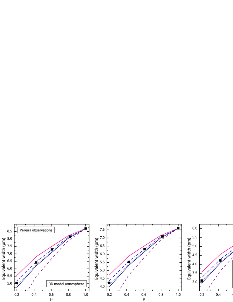
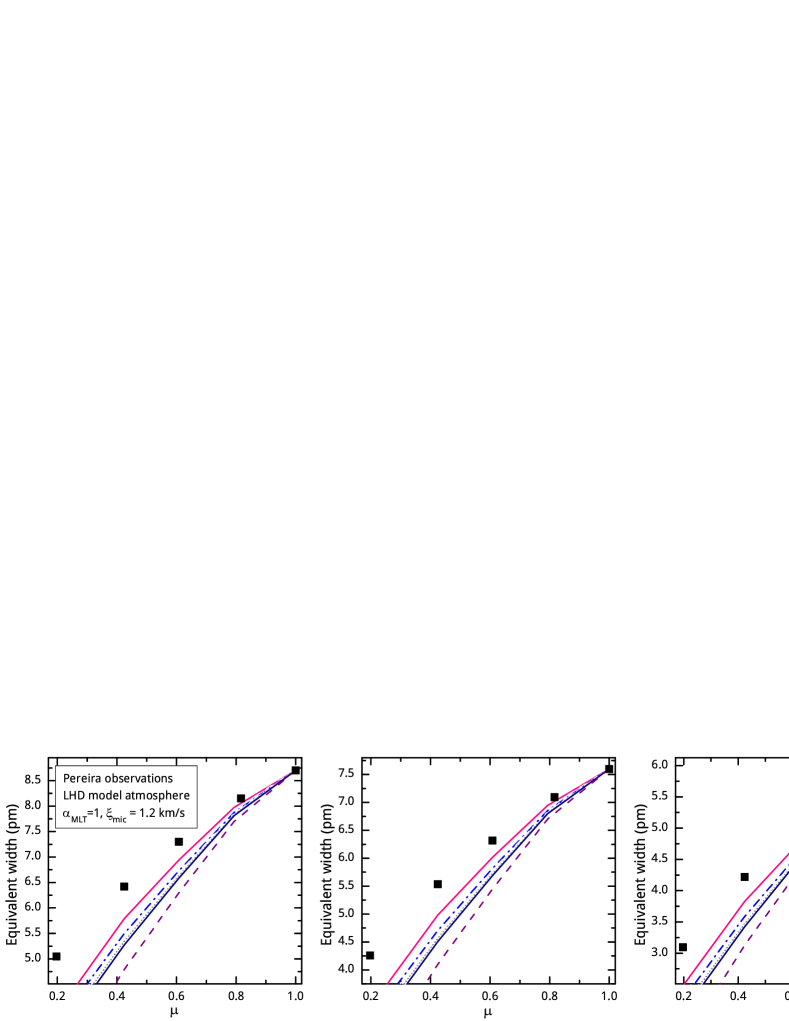
Figure 5: Center-to-limb variation of the equivalent width of the 777.4 nm (left panels) and 777.5 nm (right panels ) components of the oxygen triplet. The observed equivalent widths (black squares, Pereira et al. 2009b, a) are compared to the predictions of non-LTE line formation calculations for a 3D solar CO⁵BOLD model (top panels) and of a 1D hydrostatic (LHD) model assuming a constant, isotropic microturbulence $\xi_{\mathrm{micro}}=1.2\mbox{\rm\,km/s}$ (bottom panels). The theoretical results depend on the efficiency of collisions between oxygen and neutral hydrogen controlled by the parameter $S_{\mathrm{H}}$.

From the 3D solar model, where the hydrodynamical velocity field automatically accounts for an anisotropic, depth-dependent microturbulence, the best fit to the observations is obtained with $S_{\mathrm{H}}$ between 1.0 and 1.6 (upper panels). In contrast, the 1D LHD model with constant, isotropic microturbulence would require a negative value of $S_{\mathrm{H}}$ to reproduce the observations (lower panels), i.e. unphysical (negative) collisional cross-sections. A different choice of $\xi_{\mathrm{micro}}$ does not improve the situation. It is the assumption of a $\mu$-independent microturbulence that leads to the failure of the 1D model to reproduce the observed center-to-limb variation of the solar oxygen triplet lines. Further details can be found in Steffen et al. (2015).

3.3 Implications for stellar abundance work

The rudimentary description of the photospheric velocity field in the 1D models, together with the ignorance of horizontal temperature and pressure fluctuations, implies basic limitations of the precision of the standard abundance analysis performed with 1D models. In the following, we give a quantitative example.

Imagine you have a noiseless stellar spectrum from which you can measure the equivalent widths of a selection of iron lines with infinite precision; the atomic parameters of the lines are perfectly known. Moreover, the stellar parameters of the observed object ($T_{\mathrm{eff}}$, $\log g$, [M/H]) have already been determined independently of spectroscopy to high precision. It is also known that all iron lines form in strict LTE. Now the question is how well the known iron abundance can be reproduced from a spectroscopic analysis of the stellar spectrum using a 1D atmosphere model.

The situation described above can be investigated by identifying the synthetic spectrum of a 3D hydrodynamical model with the observation, and analyzing this spectrum in terms of the corresponding 1D model. For the example shown below, we have constructed the 1D model by averaging the 3D model on surfaces of constant Rosseland optical depth, ensuring that the temperature structure of the resulting 1D model (= $\left\langle 3D\right\rangle$ model) matches exactly the mean temperature structure of the “observed” stellar photosphere. The only deficiencies of the 1D model are its inability to account for horizontal fluctuations and its simplistic microturbulence velocity field.

Figure 6 illustrates this experiment for a subgiant with $T_{\mathrm{eff}}$ = 5500 K, $\log g$ = 3.5, and solar metallicity. The top panel shows the diagnostic plot from which the microturbulence was determined. Following common practice, $\xi_{\mathrm{micro}}$ was determined from Fe i lines with excitation potential $E>2$ eV (black diamonds) such that the trend in the 1D abundance (difference) with equivalent width is removed. Low excitation lines of Fe i and Fe ii lines are shown for further information. The average iron abundance of the microturbulence lines (dashed horizontal line) comes out close to the abundance put into the 3D synthesis. However, it is remarkable that we are left with an overall scatter of $>0.2$ dex peak-to-peak if all lines are included, even though $\xi_{\mathrm{micro}}$ has been properly adjusted, the 1D model has the correct $T_{\mathrm{eff}}$ and $\log g$, and the equivalent widths and $gf$-values of all lines are perfectly known. The residual abundance scatter must be a consequence of the imperfect representation of the photospheric velocity field by a constant microturbulence, and/or the inability of the 1D model to account for the presence of photospheric temperature fluctuations.

We further note a systematic offset between Fe i and Fe ii lines. In a classical spectroscopic analysis, this would be compensated by increasing $\log g$ of the 1D model to achieve ionization equilibrium. At the same time, there is a systematic trend with excitation potential $E$ (lower panel of Fig. 6), which would be eliminated by decreasing $T_{\mathrm{eff}}$. This example demonstrates that we must not be surprised if the spectroscopic analysis based on 1D model atmospheres yields stellar parameters that are inconsistent with the true physical parameters $T_{\mathrm{eff}}$ and $\log g$  (benchmark stars). 3D Effects of similar magnitude have been shown to exist for an F-dwarf at $T_{\mathrm{eff}}$$\,=\,$6300$\,K,\log g$ = $4.5$, [M/H]=0 by Ludwig et al. (2014).

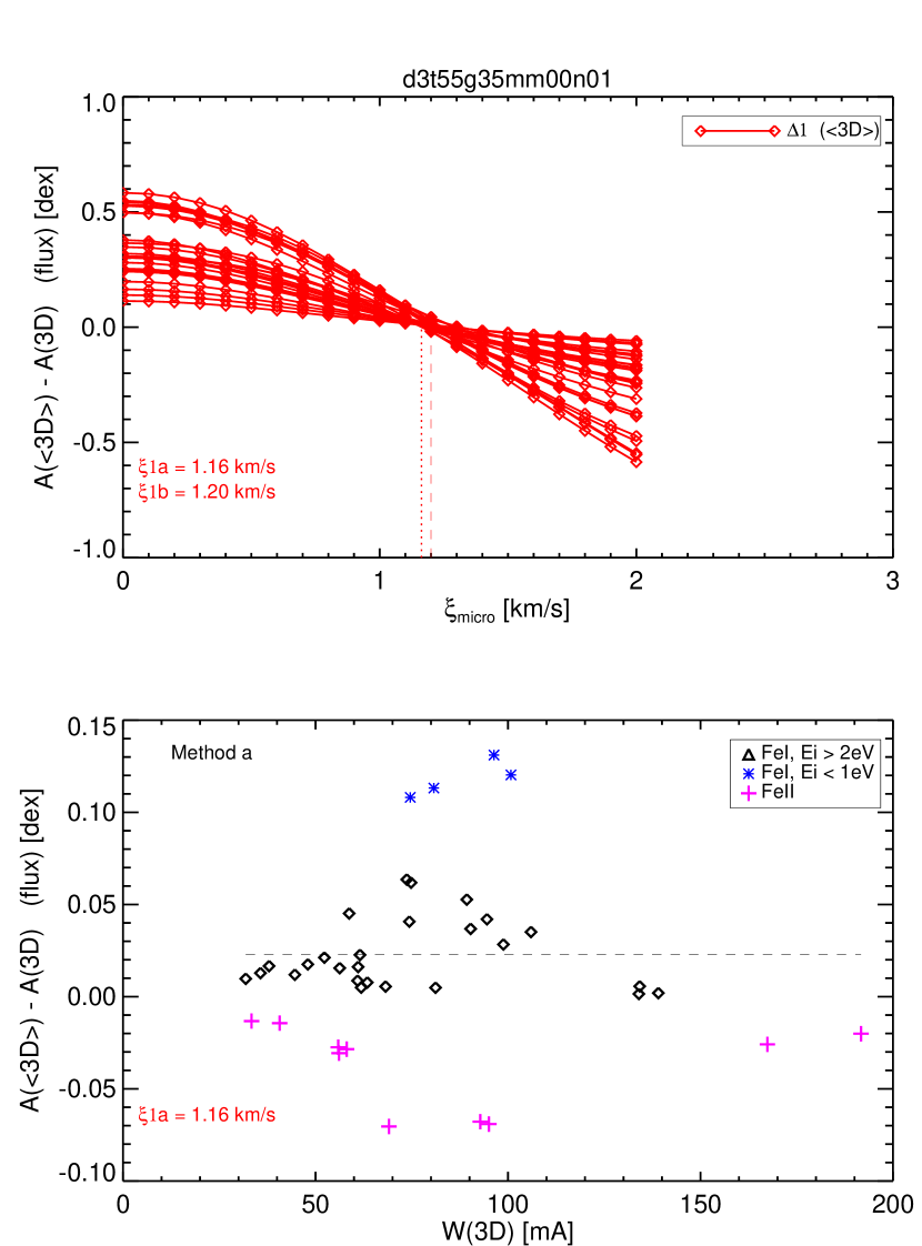
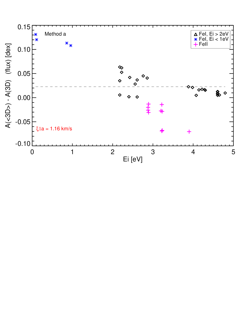
Figure 6: $\left\langle 3D\right\rangle$ $-$ 3D abundance differences for a set of Fe i and Fe ii lines versus equivalent width $W$ (top) and lower level excitation potential $E$ (bottom). $\left\langle 3D\right\rangle$ and 3D model have identical stellar parameters ($T_{\mathrm{eff}}$ = $5430$ K, $\log g=3.5$, [M/H]=0). In the $\left\langle 3D\right\rangle$ model, $\xi_{\mathrm{micro}}$ was adjusted to remove the trend of abundance with $W$ for Fe i lines with excitation potential $E>2$ eV (black diamonds).