Supplemental Material for “Bound states and field-polarized Haldane modes in a quantum spin ladder”

.1 S1. Neutron Scattering in a Two-Leg Spin Ladder

.1.1 Parity Selection

A fundamental consequence of the two-leg geometry is that all excitations of the spin ladder have an exact even or odd parity. Excitations between singlet and triplet states have odd parity ($q_{y}=\pi$ sector) and may therefore be separated systematically from excitations of inter-triplet (or inter-singlet) character, which have even parity ($q_{y}=0$ sector); this situation is represented schematically in Fig. S1. Most important for the present purposes is that one-magnon excitations are odd whereas two-magnon excitations are even; these opposite parities result in opposite phases for constructive or destructive interference, and hence in a complete separation of the maximal intensities of the two sectors in reciprocal space. A further consequence is that excitations of opposite parities do not mix, excluding the possibility of “quasiparticle breakdown” where they overlap.

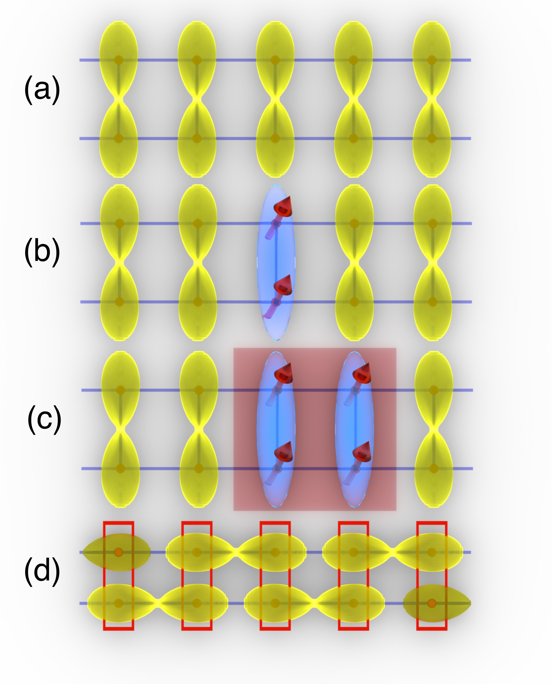
Figure S1: Schematic representation of rung states and their symmetries in spin-ladder and Haldane-chain systems at zero field. (a) Ground state of antisymmetric rung singlets in the two-leg ladder. (b) One-magnon (symmetric, triplet) excited state. (c) Two-magnon excited state; the triplet pair may be in a net singlet, triplet, or quintet ($S_{\rm tot}=0$, 1, or 2) state but its parity is equal to that of the ground state and opposite to that of the one-magnon excitation. (d) Ground state of the Haldane chain in the AKLT representation Aff87 of auxiliary $S=1/2$ spin pairs at each site; the red boxes represent the operator projecting these spins to a real $S=1$ state.

.1.2 Crystal Structure of BPCC

The structure of BPCC has the monoclinic space group P$2_{1}$/c, with lattice parameters determined by neutron diffraction at 1.6 K as $a=8.08657(5)$ Å, $b=16.57703(9)$ Å, $c=12.14457(7)$ Å, and $\beta=102.2395(4)^{\circ}$ rwea . The unit cell contains four Cu²⁺ atoms ($S=1/2$), which form two spin dimers constituting the ladder rungs, as shown in Fig. S2(a). These rung dimer units repeat periodically along the $\hat{a}$ direction, with an exchange interaction that forms the ladder legs [Fig. S2(a)]. Ladders neighboring in the $\hat{b}$ direction are related by a 2₁ screw axis and hence there are two types of spin ladder, identical (by symmetry) in their exchange interactions but different in orientation [Fig. S2(b)]. The inequivalent rung vectors are given by

$$\mathbf{r}_{1,2}=[0.3822\;\pm 0.173\>0.4866];$$ (S1)

in the same units, the leg vector is $[1\;0\;0]$. Despite this inequivalence, parity remains a good quantum number: excitations in the 0 and $\pi$ sectors are associated with geometrical phase factors expressing their constructive or destructive interference, which determine the precise locations of maximal and minimal scattering intensity throughout the Brillouin zone for each sector. Because of the monoclinic structure of BPCC, these maxima and minima are determined not solely by the reciprocal-space component, $Q_{h}$, for the ladder direction, but are found respectively at $[Q_{h}\;0\;Q_{l_{\rm max}}]$ and $[Q_{h}\;0\;Q_{l_{\rm min}}]$, where $Q_{l_{\rm max}}$ and $Q_{l_{\rm min}}$ depend on $Q_{h}$, as we discuss below.

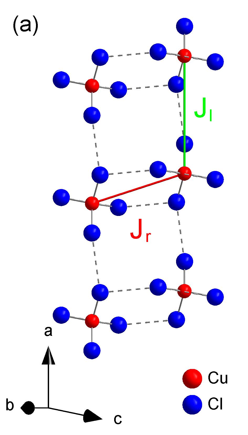
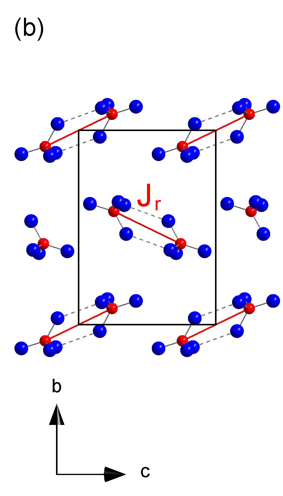
Figure S2: Representation of the crystal structure of BPCC, highlighting (a) the positions of Cu and Cl atoms in a single ladder unit and (b) the relative positions of the different ladder units, which have two different orientations; the piperidinium cations between the ladders are omitted for clarity.

.1.3 Scattering Cross-Section

The complete separation of excitations into even (0) and odd ($\pi$) parity sectors means that the neutron scattering cross section may also be decomposed into two separate types of contribution, $S^{\alpha\beta}_{0}$ and $S^{\alpha\beta}_{\pi}$ rtu . Although $\alpha$ and $\beta$ denote general spin indices, for pure Heisenberg interactions one has $S^{xx}=S^{yy}=S^{zz}=S^{+-}=S^{-+}$. When the two inequivalent wave vectors for the ladder rungs are taken into account, the total neutron scattering cross-section can be written as

$$\!\!\frac{\mathrm{d}^{2}\sigma}{\mathrm{d}\Omega\mathrm{d}E^{\prime}} \propto 4\!\left(\!\!1\!-\!\frac{Q_{z}^{2}}{Q^{2}}\!\right)\![c({\bf Q})S_{0}^{zz}\!+\!s({\bf Q})S_{\pi}^{zz}]$$

$$+\!\!\left(\!\!1\!+\!\frac{Q_{z}^{2}}{Q^{2}}\!\right)\![c({\bf Q})\!(S_{0}^{+\!-}\!\!+\!S_{0}^{-\!+})\!+\!s({\bf Q})\!(S_{\pi}^{+\!-}\!\!+\!S_{\pi}^{-\!+})],$$

where $s(\mathbf{Q})=\sum_{i=1,2}\sin^{2}(\mathbf{Q\!\cdot\!r}_{i}/2)$ and $c(\mathbf{Q})=\sum_{i=1,2}\cos^{2}(\mathbf{Q\!\cdot\!r}_{i}/2)$ are phase factors and $Q_{z}$ is the out-of-plane wave-vector component. In practice, we focus directly on the dynamical structure factor, $S(\mathbf{Q},\omega)$, extracted from $\mathrm{d}^{2}\sigma/\mathrm{d}\Omega\mathrm{d}E^{\prime}$.

Equation (.1.3) may be used to quantify the statements made in the preceding subsections. The maximum in the structure factor contributed by one-magnon excitations is found by selecting the wave vectors ${\bf Q}$ maximizing $1-\cos(\mathbf{Q\cdot r})$, where ${\bf r}={\bf r}_{1}-{\bf r}_{2}$ is the difference between the inequivalent rung vectors, i.e. ${\bf Q}$ must satisfy

$$2\pi({\bf Q\cdot r})=(2n+1)\pi,$$ (S3)

where $n$ is an integer. Conversely, the minimum in the one-magnon structure factor, which coincides with the maximum in the two-magnon (even-parity) channel, is found when $n$ takes a half-integer value. One may then deduce that

$$Q_{l}=[n+1/2-0.3822\,Q_{h}]/0.4866,$$ (S4)

with $n$ an integer for $Q_{l_{\rm max}}$ and $n$ half-integral for $Q_{l_{\rm min}}$.

This information is represented in Fig. S3, which shows the simulated structure factor of the one-magnon excitation, i.e. the quantity $S(\mathbf{Q},\omega({\bf Q}))$. The calculation of the dispersion relation, $\omega({\bf Q})$, and of the corresponding intensity is deferred to Sec. S3. The red and green solid lines mark respectively the lines of maxima and minima of the one-magnon excitations of the spin ladder, whose dynamical structure factor [$S(\mathbf{Q},\omega)$] is shown in Fig. 1(a) of the main text. As noted above, the one-magnon minimum is the two-magnon maximum, for which $S(\mathbf{Q},\omega)$ is shown in Fig. 2(a). Blue solid lines mark the maxima of the one-magnon excitations transverse to the ladder ($Q_{l}$), which are obtained at the zone boundary in $Q_{h}$ and the spin-gap energy in $\omega$, and are studied in Fig. 1(h); orange lines mark the minima, which are found at the zone center and the band maximum [Fig. 1(f)].

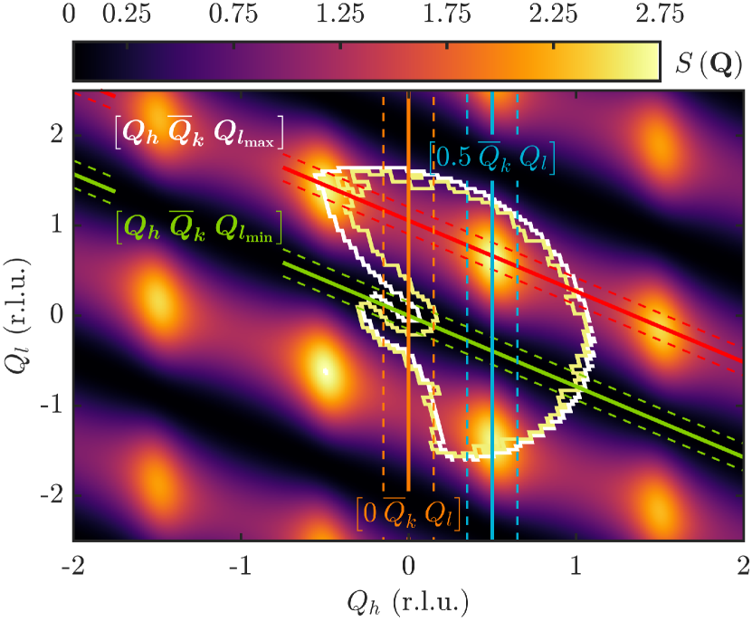
Figure S3: False-color representation of the simulated structure factor, $S(\mathbf{Q},\omega)$, of the one-magnon excitation in BPCC, calculated in a strong-coupling analysis and using the single-mode approximation (Sec. S3). The scattered intensity is shown in the horizontal scattering plane, $(Q_{h},0,Q_{l})$, for the energy value $\omega=\omega({\bf Q})$ of the one-magnon dispersion and for $Q_{k}=0$. The white line marks the full extent of the available data in $Q_{h}$ and $Q_{l}$, which is determined by the detector coverage at the energy of the one-magnon mode. At the (higher) energy of the two-magnon continuum, the detector coverage has shrunk and is shown in yellow. The other lines are described in the text.

.2 S2. Neutron Scattering Intensity Analysis

Experiments were performed on the time-of-flight spectrometer LET, with the BPCC sample mounted in the (horizontal) ac scattering plane. Data at zero applied magnetic field were collected for 104 rotation angles, corrected for detector efficiency and scattered-to-incident wave-vector ratio, $k_{f}/k_{i}$, using the MANTID program mantid , and combined into a “four-dimensional” (4D, meaning three spatial dimensions and one energy) dataset using the Matlab-based HORACE analysis code horace . The extent of the resulting dataset in reciprocal-space dimensions $Q_{h}$ and $Q_{l}$ is represented by the white line in Fig. S3. For all of the results presented in the main text, the data were integrated over the $Q_{k}$ direction, representing out-of-plane scattering, where all modes are entirely non-dispersive; we refer to the results of this integration as a 3D dataset and denote this treatment of the $Q_{k}$ direction by ${\overline{Q}}_{k}$. Further integration over directions along or across the ladder was performed to obtain the final datasets; the dashed lines in Fig. S3 mark these transverse integration ranges. In all cases, the integration range was $\pm 0.125$ r.l.u., a value achieving an acceptable signal-to-noise ratio while preserving mode coherence and sector separation.

For all quantitative analyses of the scattered intensity, we integrate $S({\bf Q},\omega)$ over a chosen window of energy to obtain the structure factor, $I({\bf Q})$. In addition to improving very significantly the signal-to-noise ratio, this procedure also allows us to select the energy range in such a way as to remove as much as possible of the contamination due to elastic and multiple scattering events. This last includes scattering from the cryomagnet, which is responsible for the parabolic intensity visible at low energies in Figs. 1(a) and 2(a). The remaining background, due to detector noise and incoherent phonon scattering, is marked by the solid black lines in Figs. 1(c) and 2(c) of the main text. Fits to the models and numerical calculations were optimized by a least-squares approach.

.2.1 Diagonal and Interladder Interactions

Exchange interactions between sites in neighboring spin ladders are reflected in the dispersion of the one-magnon mode for ${\bf Q}$ vectors transverse to the ladder axis. Any asymmetric exchange interactions within the ladder plaquettes, to which we refer here as “diagonal,” would also be manifest as a periodic modulation of the intensity distribution for the same ${\bf Q}$ vectors. Figure 1(f) shows $S({\bf Q},\omega)$ along [0 0 $Q_{l}$], where the mode is clearly non-dispersive to within the resolution of our measurements. The red line is a theoretical result (Sec. S3) with an interladder coupling of zero, and in fact the fitting process places an upper bound on interladder exchange of 0.006(1) meV. The corresponding structure factor, Fig. 1(g), is very well reproduced by calculations performed in the SMA and with DMRG. For transverse wave vectors chosen at the one-magnon gap, the dispersion is again completely flat [Fig. 1(h)] and the structure factor is described perfectly by a system of pure and isolated ladders [Fig. 1(i)]. Again there is no discernible periodicity, in dispersion or intensity, within the instrumental resolution, placing the same limit, 0.006(1) meV, on any possible diagonal or interladder interactions.

.3 S3. Theoretical Analysis of Strong-Rung Ladders

.3.1 One-Magnon Dispersion

Several theoretical approaches are known to give good descriptions of the two-leg ladder in the strong-rung regime, including a direct perturbative expansion Rei94 and the bond-operator formalism rnr . Numerically, both exact diagonalization (ED) and DMRG work well because of the short correlation length of the well-gapped system Rue08 . In terms of the parameter $\gamma=J_{l}/J_{r}$, to third order in a perturbative expansion one obtains the dispersion relation Rei94

$$\frac{\omega(q)}{J_{r}} = 1+\frac{3}{4}\gamma^{2}+\frac{3}{8}\gamma^{3}+\left(\!\gamma-\frac{1}{4}\gamma^{3}\!\right)\!\cos q$$ (S5)

$$-\frac{1}{4}\!\left(\gamma^{2}+\gamma^{3}\right)\cos 2q+\frac{1}{8}\gamma^{3}\cos 3q$$

for the elementary triplet (one-magnon) excitation, where we have defined $q=2\pi Q_{h}$. In the bond-operator description, the dispersion is given by

$$\omega(q)=\sqrt{({\textstyle\frac{1}{4}}J_{r}-\mu)({\textstyle\frac{1}{4}}J_{r}-\mu+2J_{l}{\overline{s}}^{2}\cos q)},$$ (S6)

where the $\mu$ is the chemical potential for the triplet excitations, which are hard-core bosons, and ${\overline{s}}$ expresses the extent to which the ground state is one of pure rung singlets rnr .

.3.2 Single-Mode Approximation

While Eq. (.1.3) is an expression for the total neutron scattering cross-section, in many gapped quantum magnets the overwhelming majority of the scattered intensity can be found in the one-magnon branch of the excitation spectrum. In this situation, a meaningful analysis of the spectral weight is obtained within the single-mode approximation (SMA) Xu00 . Quite generally, the first-moment sum rule relates the integrated spectral weight of a spin ladder to the equal-time correlation functions in the form

$$\!\!\!\!\int\!\!d\omega \,\hbar\omega S(\mathbf{Q},\omega)=-{\textstyle\frac{2}{3}}(J_{r}\langle\mathbf{S}_{i}^{m}\!\cdot\mathbf{S}_{i}^{n}\rangle[1-\cos(\mathbf{Q\!\cdot d})]$$

$$+J_{l}(\langle\mathbf{S}_{i}^{m}\!\cdot\mathbf{S}_{i+1}^{m}\rangle+\langle\mathbf{S}_{i}^{n}\!\cdot\mathbf{S}_{i+1}^{n}\rangle)[1-\cos(\mathbf{Q\!\cdot r}_{l})]),$$

where $m$ and $n$ denote the two chains of the ladder, $\mathbf{d}=\mathbf{r}_{m}-\mathbf{r}_{n}$ is the dimer (rung) bond vector and ${\mathbf{r}}_{l}=\mathbf{r}_{m,i+1}-\mathbf{r}_{m,i}$ is the leg bond vector. In the SMA, the integral over $\omega$ includes a $\delta$-function, $\delta(\omega-\omega({\bf Q}))$, which transforms the left-hand side into a simple product of $\omega({\bf Q})$ and the structure factor, $I({\bf Q})$. The right-hand side is a set of “bond energies,” weighted by cosine factors determined from the geometry of the system. These bond energies are the product of the exchange interactions for each bond with the average bond spin correlations.

As noted in the main text, $J_{r}$ and $J_{l}$ for BPCC can be established independently by using the one-magnon dispersion, and therefore one would wish to determine the average spin correlations on the rung and leg bonds directly from the experimental dataset. For guidance, by performing ED calculations on ladders of coupling ratio $\gamma=0.39$ and up to $2\times 12$ spins using the ALPS package alps , we determine the average rung spin correlations, $\langle\mathbf{S}_{i}^{m}\cdot\mathbf{S}_{i}^{n}\rangle=-0.6740$, and leg correlations, $\langle\mathbf{S}_{i}^{m}\cdot\mathbf{S}_{i+1}^{m}\rangle=\langle\mathbf{S}_{i}^{n}\cdot\mathbf{S}_{i+1}^{n}\rangle=-0.1816$. However, because of an unknown intensity scale factor, only the ratio of these correlations can be extracted from the measured integrated intensities. From the reduced dataset, we deduce the ratio $\langle\mathbf{S}_{i}^{m}\cdot\mathbf{S}_{i+1}^{m}\rangle/\langle\mathbf{S}_{i}^{m}\cdot\mathbf{S}_{i}^{n}\rangle=0.22(1)$, which compares favorably with the ratios 0.2586, given within the bond-operator formalism rnr , and 0.2694 obtained from ED. The structure factors obtained in the SMA by using these average bond correlation values are entirely consistent with the measured intensities, as shown by the black, dashed lines in Figs. 1(c), 1(g), and 1(i).

.3.3 Density-Matrix Renormalization Group

DMRG calculations of the dynamical structure factor of an ideal spin ladder were performed in both the $q_{y}=0$ and $\pi$ sectors using the optimized exchange interaction parameters $J_{r}$ = 0.295 meV and $J_{l}$ = 0.115 meV. The calculations used the time-dependent DMRG method Vid04 ; WF04 ; DV04 ; Sch11 to determine the spatial spin correlation functions at zero temperature in real-time for a ladder of 200 rungs. They employed a fixed maximal number of a few hundred states and a maximal simulation time of 200 $\hbar/J_{r}$, with a time-step typically taken as $\delta t=0.2\hbar/J_{r}$. These choices ensured that the remaining errors were sufficiently small as to have no discernible effect on the primary spectral structures. The dynamical spin correlations in momentum space were obtained by Fourier transformation of the spin correlation functions. More details of the calculational procedure are described in Refs. Bou11 ; rbu .

The spectra obtained in this way were convolved with a Gaussian function representing the instrumental resolution, combined using Eq. (.1.3), weighted by the magnetic form factor of Cu²⁺, and added to a constant background value extracted from the experimental dataset. By this process we formed a DMRG dataset for $S({\bf Q},\omega)$ completely equivalent to the experimental one. This DMRG dataset was cut, integrated in ${\bf Q}$, and integrated in $\omega$ using precisely the same techniques as described above. The results are displayed both as the color contours in Figs. 1(b) and 2(b) of the main text [for $S({\bf Q},\omega)$] and as the solid lines in Figs. 1(c), 1(g), 1(i), and 2(c) [for $I({\bf Q})$].

.3.4 High-Order Series Expansions

The systematic extension of the strong-coupling approximation is the high-order series-expansion method, which has been applied previously for the calculation of bound states and dynamical correlation functions in quantum spin ladders Zhe01 ; Kne01 . Here we have used perturbative continuous unitary transformations (pCUTs) Kne00 ; Kne01 to map the spin ladder order by order in $\gamma$ to an effective Hamiltonian, $\mathcal{H}_{\rm eff}$, which conserves the number of elementary $S=1$ excitations. Physically, the $\gamma=0$ ground state is the product state of rung singlets and the elementary excitation is a rung triplet; at finite $\gamma$, these triplets become dressed by their mutual interactions to yield the elementary magnon excitations.

Because $\mathcal{H}_{\rm eff}$ conserves the magnon number, each (interacting) few-magnon problem can be addressed separately. Here we have determined the one-magnon hopping amplitudes up to order 11 in $\gamma$, the two-magnon interaction amplitudes with $S_{\rm tot}=1$ up to order 10, and the matrix elements in the one- and two-magnon channels relevant for $S({\bf Q},\omega)$ also to 10th order. All series are essentially converged for $\gamma=0.39$ and no extrapolations are required. The one-magnon sector is readily diagonalized by Fourier transformation to give the one-magnon dispersion and spectral weight directly.

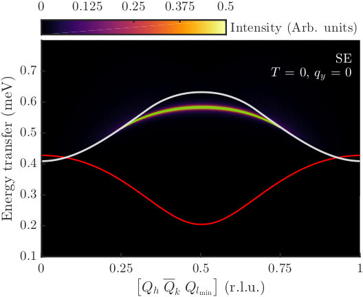
Figure S4: Dynamical structure factor, $S({\bf Q},\omega)$, in the symmetric ($q_{y}=0$) sector, calculated by series-expansion (SE) methods up to 10th order, showing the triplet component of the two-magnon bound state and the absence of visible intensity from the two-magnon continuum. The red line marks the one-magnon dispersion and the white line the lower boundary of the two-magnon continuum.

In the two-magnon channel, it is necessary to solve a two-body problem to obtain $S({\bf Q},\omega)$ Kne04 , which we execute by Lanczos tridiagonalization of the two-magnon $\mathcal{H}_{\rm eff}$ for fixed total momentum ${\bf Q}$. The only remaining degree of freedom is the separation, $d$, of the two magnons, and by allowing a maximal $d=4000$ all finite-size effects are essentially eliminated from the calculation. From the Lanczos tridiagonalization, we extract Kne04 the complete two-magnon contribution to $S({\bf Q},\omega)$, the dispersion and the intensity of the two-magnon bound state as a function of ${\bf Q}$, and the corresponding intensity of the two-magnon continuum. We note that the two-magnon structure factor, $I({\bf Q})$, corresponds to the sum of bound-state and continuum contributions and is obtained directly from the matrix elements.

As for our DMRG calculations, to obtain a dataset comparable with experiment we scale and smooth our series-expansion data for $S({\bf Q},\omega)$ and integrate them in the same manner. Focusing on the results for the two-magnon triplet bound state, in Fig. S4 we show $S({\bf Q},\omega)$ calculated in the $q_{y}=0$ sector and in Fig. 2(c) of the main text the corresponding $I({\bf Q})$ for comparison with the results from experimental measurements and DMRG calculations.

.3.5 Two-Magnon Bound States

For an accurate description of the two-magnon bound state we employ the strong-coupling series expansion Zhe01 ; Kne01 . For illustration, the energy of the triplet component of the bound state is given to third order by

$$\frac{\omega_{B}(q)}{J_{r}} = 2\!-\!\frac{3}{2}\gamma\!+\!\frac{11}{8}\gamma^{2}\!+\!\frac{17}{16}\gamma^{3}\!-\left(\!\gamma\!+\!\frac{1}{4}\gamma^{2}-\frac{9}{16}\gamma^{3}\!\right)\cos q$$ (S8)

$$-\frac{1}{2}(\gamma^{2}+\gamma^{3})\cos 2q-\frac{5}{16}\gamma^{3}\cos 3q.$$

In the same approximation, the lower edge of the two-magnon continuum is located at the energy

$$\frac{\omega_{2m}(q)}{J_{r}} = 2\!+\!\frac{3}{2}\gamma^{2}\!+\!\frac{3}{4}\gamma^{3}\!-2\left(\!\gamma\!-\!\frac{1}{4}\gamma^{3}\!\right)\!\cos{\textstyle\frac{1}{2}}q$$ (S9)

$$-\frac{1}{2}(\gamma^{2}+\gamma^{3})\cos q-\frac{1}{4}\gamma^{3}\cos{\textstyle\frac{3}{2}}q.$$

One observes that the triplet bound states are cut off by the presence of the continuum, but exist over a range of wave vectors $q_{c}\leq q\leq 2\pi-q_{c}$ around the edges of the Brillouin zone, where $q_{c}=2\pi Q_{c}$ is given in Eq. (1) of the main text. For ladders with stronger rung-to-leg coupling ratio (weaker $\gamma$), $q_{c}\simeq 2\pi/3$ and the bound state is restricted to the outer 1/3 of the 1D Brillouin zone. For larger $\gamma$ values, the range over which the bound-state mode exists (1) becomes slightly larger Zhe01 and so does its separation in energy from the continuum edge. However, the primary factor affecting its visibility is the intensity of the two-magnon continuum, which rises significantly more strongly than the energetic separation. The very weak two-magnon continuum [Figs. S4 and 2(c)] is therefore the reason why the bound state is so much more clearly visible in BPCC than in any other systems studied previously.

Quantitatively, as discussed in the main text we find that, even for a coupling ratio as apparently modest as $\gamma\simeq 0.4$, a 10th-order expansion is required for an accurate account of the relative positions of the bound state and the continuum edge for a pair of magnons. In our analysis of the scattering intensities in Fig. 2(c), we compute the structure factor by integrating over an energy window up to the two-magnon continuum boundary and attribute these contributions to the bound state. The energy window above the continuum edge is attributed to two-magnon scattering states. It is clear that applying the same process to our $S({\bf Q},\omega)$ data, calculated both by DMRG and by series expansions, gives an excellent quantitative account of the measured intensities.

We remark here that one of the open questions under these circumstances concerns the “termination” of the bound-state mode where it meets the continuum at the cut-off wave vector, $q_{c}$. As noted in the main text, the termination of the one-magnon mode in the two-magnon continuum, as discussed in Ref. Sto06 , is precluded in BPCC by their opposite parities. However, both bound and scattering states of two magnons appear in the same parity sector ($q_{y}=0$), and thus there is no parity protection for the bound state in this situation. To understand whether the bound state ceases to exist as a well-defined excitation of the system at $q_{c}$, before it, or persists in some form into the two-magnon continuum, it is necessary to analyze the line width of this spectral feature; a structure-factor analysis of the type performed in Fig. 2(c) does not address the origin of the intensity contributions. Unfortunately, the data quality of our experimental measurements is not sufficient for a quantitative discussion of this issue. Numerically, both our DMRG and series-expansion calculations may be used to investigate the nature of this termination, which, however, lies beyond the scope of the present analysis.

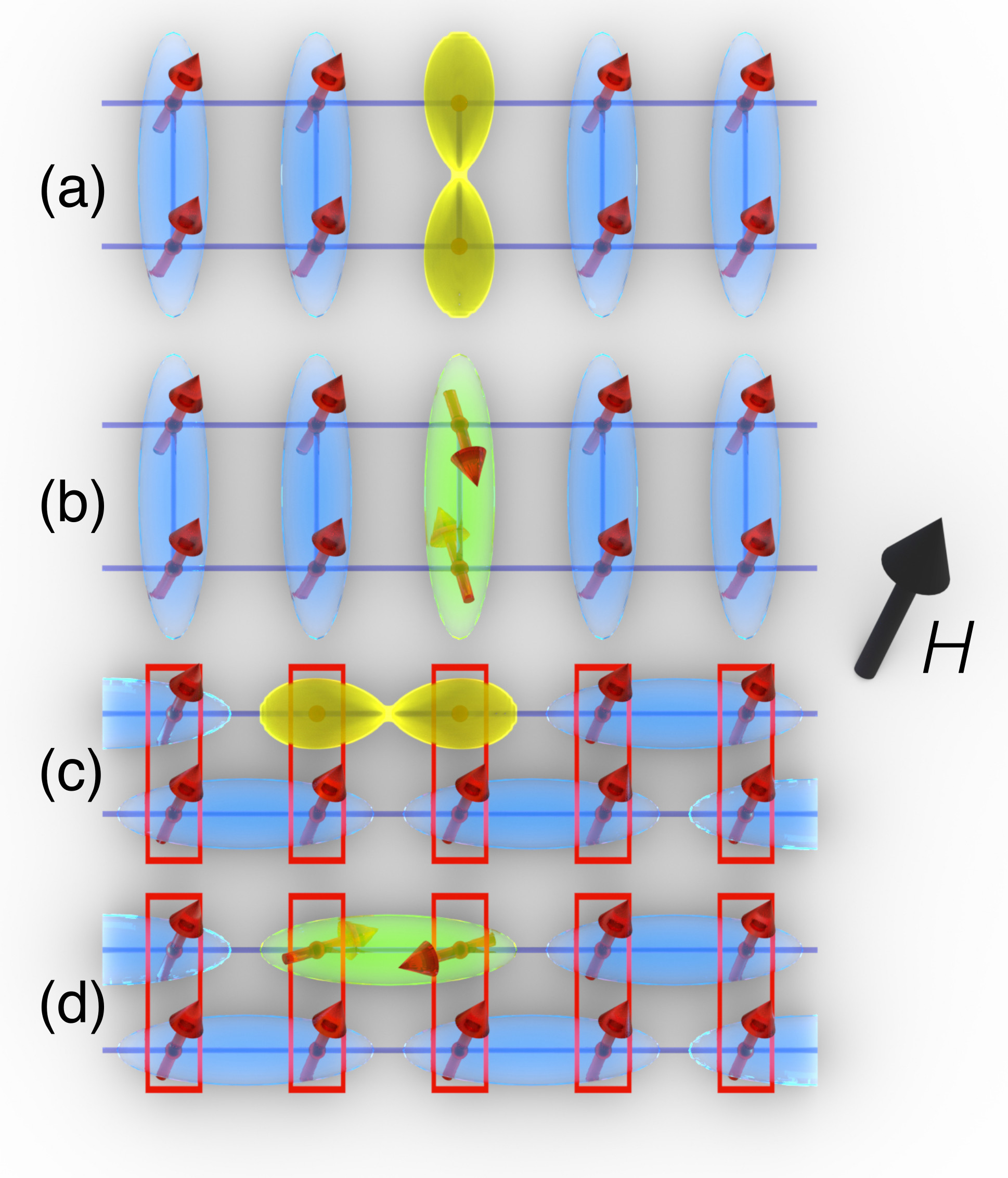
Figure S5: Schematic representation of the rung states and their symmetries in fully field-polarized spin-ladder and Haldane-chain systems. (a) Polarized two-leg ladder with one rung-singlet excitation. (b) Polarized ladder with one rung-triplet ($t_{0}$) excitation. Polarized Haldane chain in the AKLT representation containing (c) one bond-singlet excitation and (d) one $t_{0}$ bond-triplet excitation.

.3.6 Field-Polarized Phase

The most straightforward description of the fully polarized (FP) phase is obtained by using the bond-operator description. For magnetic fields beyond the saturation field, $h_{s}=g\mu_{\rm B}H_{s}$, there are one singlet and two triplet excitations, while the third triplet, $t_{+}$, is the ground state and therefore is treated as fully condensed, i.e. $\langle t_{+}\rangle={\overline{t}}$ is a constant. From the Hamiltonian,

$$H = \sum_{i}\left[(-{\textstyle\frac{3}{4}}J_{r}-\mu)s_{i}^{\dagger}s_{i}+({\textstyle\frac{1}{4}}J_{r}-\mu+h)t_{+i}^{\dagger}t_{+i}\right.$$

$$+\left.({\textstyle\frac{1}{4}}J_{r}-\mu)t_{0i}^{\dagger}t_{0i}+({\textstyle\frac{1}{4}}J_{r}-\mu-h){\overline{t}}^{2}+\mu+{\textstyle\frac{1}{2}}J_{l}{\overline{t}^{4}}\right]$$

$$+{\textstyle\frac{1}{2}}J_{l}\sum_{i}\left[{\overline{t}}^{2}(s_{i}^{\dagger}s_{i+1}+t_{0i}^{\dagger}t_{0i+1}+{\rm H.c.})-2{\overline{t}}^{2}t_{-i}^{\dagger}t_{-i}\right],$$

one may extract the mean-field equations

$$\frac{\partial H}{\partial\mu} = 0\,=\,1-{\overline{t}}^{2},$$ (S11)

$$\frac{\partial H}{\partial{\overline{t}}^{2}} = 0\,=\,{\textstyle\frac{1}{4}}J_{r}-\mu-h+J_{l}{\overline{t}}^{2},$$ (S12)

and hence conclude that ${\overline{t}}=1$ exactly, which is the bond-operator expression of the fact that quantum fluctuations are completely suppressed in the saturated regime. This has the important consequence that the elementary excitations are truly non-interacting and hence the exchange parameters deduced from their dispersion may be used as a benchmark for cases where interaction effects are unknown Col02 .

Further, the chemical potential, $\mu={\textstyle\frac{1}{4}}J_{r}+J_{l}-h$, is governed only by the applied field, $h$ (contributions from the sinusoidal excitation bands sum to zero). Thus the dispersion relations are

$$\!\!\omega_{s}(q) = -{\textstyle\frac{3}{4}}J_{r}-\mu+J_{l}{\overline{t}}^{2}\!\cos k=h-J_{r}-J_{l}(1\!-\!\cos q),$$

$$\!\!\omega_{0}(q) = {\textstyle\frac{1}{4}}J_{r}-\mu+J_{l}{\overline{t}}^{2}\!\cos k=h-J_{l}(1-\cos q),$$ (S13)

$$\!\!\omega_{-}(q) = {\textstyle\frac{1}{4}}J_{r}-\mu+h-J_{l}{\overline{t}}^{2}=2h-2J_{l}.$$

The rung-singlet excitation, $\omega_{s}(q)$, is represented schematically in real space in Fig. S5(a) and the lowest rung-triplet mode, $\omega_{0}(q)$, in Fig. S5(b). The upper mode, $\omega_{-}$, is completely non-dispersive (the band narrows to zero as $h$ increases to $h_{s}$). The lower mode satisfies $\omega_{s}(q)=0$ at the band minimum at the saturation field, defining $h_{s}=J_{r}+2J_{l}$, as expected from simple considerations of saturating all the bonds at a single site (no quantum fluctuations and thus no correlation effects). These expressions allow a very accurate fit of the exchange parameters in the FP regime, as reported in the main text, with no requirement for any extra terms in the magnetic Hamiltonian beyond those of the pure Heisenberg spin ladder. The small deviations of the high-field $J_{r}$ and $J_{l}$ parameters from their zero-field values are magnetostriction effects, which as in BPCB are weak Thi09a . Figures S5(c) and S5(d) illustrate the close similarity of the FP-phase excitations of the Haldane chain to those of the two-leg ladder.

References

- (1) S. Ward, S. Furuya, D. Biner, K. W. Krämer, D. Cheptiakov, M. Boehm, D. F. McMorrow, T. Giamarchi, and Ch. Rüegg, unpublished.
- (2) I. Affleck, T. Kennedy, E. H. Lieb, and H. Tasaki, Phys. Rev. Lett. 59, 799 (1987); Commun. Math. Phys. 115, 477 (1988).
- (3) B. Thielemann, Ph. D. thesis, ETH Zurich (2009).
- (4) Available at http://www.mantidproject.org.
- (5) R. A. Ewings, A. Buts, M. D. Le, J. van Duijn, I. Bustinduy, and T. G. Perring, Nuclear Instruments and Methods in Physics Research Section A: Accelerators, Spectrometers, Detectors and Associated Equipment 834, 132 (2016).
- (6) M. Reigrotzki, H. Tsunetsugu, and T. M. Rice, J. Phys.: Condens. Matter 6, 9235 (1994).
- (7) B. Normand and Ch. Rüegg, Phys. Rev. B 83, 054415 (2011).
- (8) Ch. Rüegg, K. Kiefer, B. Thielemann, D. F. McMorrow, V. Zapf, B. Normand, M. B. Zvonarev, P. Bouillot, C. Kollath, T. Giamarchi, S. Capponi, D. Poilblanc, D. Biner, and K. W. Krämer, Phys. Rev. Lett. 101, 247202 (2008).
- (9) G. Xu, C. Broholm, D. H. Reich, and M. A. Adams, Phys. Rev. Lett. 84, 4465 (2000).
- (10) B. Bauer, L. D. Carr, H. G. Evertz, A. Feiguin, J. Freire, S. Fuchs, L. Gamper, J. Gukelberger, E. Gull, S. Guertler, A. Hehn, R. Igarashi, S. V. Isakov, D. Koop, P. N. Ma, P. Mates, H. Matsuo, O. Parcollet, G. Pawlowski, J. D. Picon, L. Pollet, E. Santos, V. W. Scarola, U. Schollwöck, C. Silva, B. Surer, S. Todo, S. Trebst, M. Troyer, M. L. Wall, P. Werner, and S. Wessel, J. Stat. Mech. P05001 (2011).
- (11) G. Vidal, Phys. Rev. Lett. 93, 040502 (2004).
- (12) S. R. White and A. E. Feiguin, Phys. Rev. Lett. 93, 076401 (2004).
- (13) A. J. Daley, C. Kollath, U. Schollwöck, and G. Vidal, J. Stat. Mech.: Theor. Exp. P04005 (2004).
- (14) U. Schollwöck, Ann. Phys. 326, 96 (2011).
- (15) P. Bouillot, C. Kollath, A. M. Läuchli, M. Zvonarev, B. Thielemann, Ch. Rüegg, E. Orignac, R. Citro, M. Klanjšek, C. Berthier, M. Horvatić, and T. Giamarchi, Phys. Rev. B 83, 054407 (2011).
- (16) P. Bouillot, Ph. D. thesis, University of Geneva (2011).
- (17) W. Zheng, C. J. Hamer, R. R. P. Singh, S. Trebst, and H. Monien, Phys. Rev. B 63, 144410 (2001).
- (18) C. Knetter, K. P. Schmidt, M. Grüninger, and G. S. Uhrig, Phys. Rev. Lett. 87, 167204 (2001).
- (19) C. Knetter and G. S. Uhrig, Eur. Phys. J. B 13, 209 (2000).
- (20) C. Knetter, K. P. Schmidt, and G. S. Uhrig, Eur. Phys. J. B 36, 525 (2004).
- (21) M. B. Stone, I. A. Zaliznyak, T. Hong, C. L. Broholm, and D. H. Reich, Nature 440, 187 (2006).
- (22) R. Coldea, D. A. Tennant, K. Habicht, P. Smeibidl, C. Wolters, and Z. Tylczynski, Phys. Rev. Lett. 88, 137203 (2002).
- (23) B. Thielemann, Ch. Rüegg, H. Rønnow, A. M. Läuchli, J. S. Caux, B. Normand, D. Biner, K. W. Krämer, H. U. Güdel, J. Stahn, K. Habicht, K. Kiefer, M. Boehm, D. F. McMorrow, and J. Mesot, Phys. Rev. Lett. 102, 107204 (2009).