Time-series Doppler images and surface differential rotation of the effectively-single rapidly-rotating K-giant KU Pegasi

Abstract

Context. According to most stellar dynamo theories, differential rotation (DR) plays a crucial role for the generation of toroidal magnetic fields. Numerical models predict surface differential rotation to be anti-solar for rapidly-rotating giant stars, i.e., their surface angular velocity could increase with stellar latitude. However, surface differential rotation has been derived only for a handful of individual giant stars to date.

Aims. The spotted surface of the K-giant KU Pegasi is investigated in order to detect its time evolution and quantify surface differential rotation.

Methods. We present altogether 11 Doppler images from spectroscopic data collected with the robotic telescope STELLA between 2006–2011. All maps are obtained with the surface reconstruction code iMap. Differential rotation is extracted from these images by detecting systematic (latitude-dependent) spot displacements. We apply a cross-correlation technique to find the best differential rotation law.

Results. The surface of KU Peg shows cool spots at all latitudes and one persistent warm spot at high latitude. A small cool polar spot exists for most but not all of the epochs. Re-identification of spots in at least two consecutive maps is mostly possible only at mid and high latitudes and thus restricts the differential-rotation determination mainly to these latitudes. Our cross-correlation analysis reveals solar-like differential rotation with a surface shear of $\alpha=+0.040\pm 0.006$, i.e., approximately five times weaker than on the Sun. We also derive a more accurate and consistent set of stellar parameters for KU Peg including a small Li abundance of ten times less than solar.

1 Introduction

Quantifying differential surface rotation has proven difficult even for the Sun. Stellar observations are even more demanding and correspondingly ambiguous are the results. However, quantitative detections are now possible for those stars where we are able to spatially resolve the stellar disk by means of Doppler imaging. Such observations (e.g., Korhonen et al., 2007; Weber, 2007; Kővári et al., 2013, 2015, etc.) as well as theoretical considerations (Kitchatinov & Rüdiger, 2004; Küker & Rüdiger, 2012) imply that stellar surface rotation could probably be more complex for evolved stars when compared to main sequence stars like the Sun. Differential rotation for main-sequence and pre-main sequence stars is found to decrease with effective temperature (Barnes et al., 2005; Reinhold et al., 2013) just like predicted from mean-field dynamo models (Küker, 2015). However, the situation seems to be less well defined for post-main sequence stars with their much deeper convective envelopes. Because many of these giants are components in RS CVn-type binary systems, their surfaces are possibly distorted by and respond to the orbital dynamics. Moreover, as a star evolves up the red-giant branch, its core experiences a modification of nuclear reactions followed by core contraction and envelope expansion long before helium burning sets in. After the core hydrogen is exhausted, the hydrogen fusion keeps going in a surrounding shell, providing more helium onto the contracting inert core. The contraction heats up the core together with the interlocked shell, which expands inward. At a point the core becomes degenerate. The increasing density at the bottom of the H-rich shell yields a more efficient H-burning, which eventually blows up the envelope. The temperature of the envelope decreases and the outer layers become fully convective, transporting more flux outwards, which explains the rapidly increasing luminosity with decreasing surface temperature along the RGB. The shell material penetrates into the hotter regions below, decaying light elements and triggering a mixing process called the first dredge up, which is responsible for the dilution of the lithium. Indeed, according to Charbonnel (1994, 1995) in low mass ($\leq 2M_{\odot}$) stars, further rotationally induced mixing occurs after the completion of the first dredge up (see also Zahn, 1992). Such mixing episodes can be inferred from the lowering of the observed surface abundances of the most fragile elements (⁷Li, ¹²C) and the ¹²C/¹³C isotopic ratio (Gratton et al., 2000). Even the simple expansion appears to have an effect on the mixing of the convective envelope and eventually also alters the surface DR profile as well. In some cases, the DR profile can be even of anti-solar type, i.e., the equator rotating slower than the poles (Vogt & Hatzes, 1991; Strassmeier et al., 2003; Kővári et al., 2015, etc.). Whether such anti-solar DR was already present during the main sequence phase of such a star or explicitly developed during the expansion phase on the giant branch is not known. Besides, DR of either solar or anti-solar has been derived only for a handful of late-type evolved stars to date. A short list of the giant stars with known DR from Doppler imaging would include the following ones. Among the single (or effectively single) giants, solar type DR was reported for FK Com (Korhonen et al., 2007), V390 Aur (Konstantinova-Antova et al., 2012) and KU Peg (Weber & Strassmeier, 2001), i.e., the star to be revisited in this paper, while anti-solar DR was detected on HD 31993 (Strassmeier et al., 2003), DI Psc and DP CVn (Kővári et al., 2013; Kriskovics et al., 2014). In binary systems solar type DR was found e.g., on the evolved components of $\zeta$ And (Kővári et al., 2012), XX Tri (Künstler et al., 2015), and IL Hya (Kővári et al., 2014), while anti-solar DR was found on $\sigma$ Gem (Kővári et al., 2015), IM Peg, UZ Lib, etc. (see Kővári & Oláh, 2014, and the references therein). Our foremost aim is to enlarge the observational sample of reliable DR detections on giant stars.

Time-series Doppler imaging has proven to be extremely useful for studying stellar DR (e.g. Vogt & Hatzes, 1996; Donati & Collier Cameron, 1997; Weber & Strassmeier, 1998; Petit et al., 2004). When having subsequent Doppler reconstructions of the spotted stellar surface, the rotation rates of individual spots can reveal the latitude-dependent stellar rotation profile. However, such Doppler reconstructions require high-resolution spectroscopic time-series data, covering at least two but better many consecutive rotation cycles. That this is indeed a challenge for stars with rotation periods of close to a month is obvious. A unique possibility for such long-term Doppler observations (see, e.g., Kővári et al., 2015; Strassmeier et al., 2015; Künstler et al., 2015, etc.) is provided by the STELLA robotic observatory of the AIP in Tenerife (Strassmeier et al., 2010). In this paper we present and analyze such spectroscopic observations of the rapidly-rotating ($P_{\rm rot}\approx 24$ days) K-giant KU~Peg (=HD 218153).

Chromospheric activity of KU Peg was recognized by Bidelman (1983) who reported strong Ca ii H&K emission. The large chromospheric fluxes were later confirmed with IUE observations by de Medeiros et al. (1992). Just recently, Aurière et al. (2015) detected magnetic fields on KU Peg and found that the star follows the magnetic field strength-rotation relationship established for active giants, indicating that probably a solar type magnetic dynamo was working inside. In addition, the authors reported an unusually strong X-ray luminosity of $L_{X}=11.8\times 10^{30}$ erg s^-1 confirming the existence of coronal activity as well. KU Peg was found to be a single-lined spectroscopic binary with an orbital period of $\approx$1400 days (de Medeiros et al., 1992), suggesting that it is effectively a single star. Because differential rotation is supposed to be weakened (or totally quenched) by tidal forces in close binaries (Scharlemann, 1981, 1982), KU Peg is a good candidate for a comparison with theory. A projected rotational velocity of 29  km s^-1 was measured by Fekel (1997), which placed the star among the possible Doppler-imaging candidates (Strassmeier et al., 2000).

The first and so far only Doppler-imaging study of KU Peg was carried out by Weber & Strassmeier (2001, hereafter Paper I) using high-resolution spectra taken with the McMath-Pierce solar telescope and the coudé feed telescope at Kitt Peak National Observatory over two months in 1996/97. The data allowed the reconstruction of two consecutive Doppler images that revealed an asymmetric polar spot and several other cool spots at lower latitudes. The time evolution of the spotted surface was followed by means of a cross-correlation analysis and revealed a complex DR profile that resembled the solar case only in the directional sense, i.e., lower latitudes rotating faster. Its lap time was twice as long as that of the Sun for the full pole-to-equator range but twice as short if only the latitudes where the Sun has spots was considered. Moreover, patterns of local meridional flows were detected, which likely play also an important role for stellar dynamos (Kitchatinov & Rüdiger, 2004; Küker & Rüdiger, 2011).

The current paper is organized as follows. In Sect. 2 we describe our photometric and spectroscopic observations. In Sect. 3 photometric data from more than 18 years are employed to derive a precise average rotation period. These data are also used to search for photometric signals of surface DR. In Sect. 4, we first redetermine the basic astrophysical properties of KU Peg by including our new photometric and spectroscopic data. Then we give a brief description of our inversion code iMap and its data assumptions for image reconstruction and, thirdly, we present the time-series Doppler images. In Sect. 5 the consecutive Doppler images are used to derive the surface DR of KU Peg. Lithium abundance determination is carried out in Sect. 6. The results are summarized and discussed in Sect. 7.

2 Observations

2.1 Photometry

Photometric observations in this paper were obtained with the Amadeus 0.75 m automatic photoelectric telescope (T7-APT) of the AIP operated at Fairborn Observatory in southern Arizona (Strassmeier et al., 1997). The data set consists of altogether 1243 measurements in Johnson $V$ and 1306 measurements in the Johnson-Cousins $I_{C}$ band. A total of, so far, 18 years between JD 2 450 395 and 2 457 015 are covered. Differential photometric observations were carried out with respect to HD 218610 as the comparison star ($V=7\aas@@fstack{m}7940$, $V-I=1\aas@@fstack{m}34$), and HD 219050 as the check star. Mean photometric errors were $0\aas@@fstack{m}006$ in $V$ and $0\aas@@fstack{m}009$ in $I_{C}$. For more details on APT performance and operation, as well as its data reduction, we refer to Granzer et al. (2001).

2.2 Spectroscopy

A total of 193 high-resolution spectra were collected with the robotic 1.2 m STELLA-I telescope at the Izaña Observatory in Tenerife, Spain (Strassmeier et al., 2010) during 2006–2011. The STELLA robotic observatory (also containing a 1.2 m photometric telescope, now STELLA-I) runs fully autonomous without any personnel on site just guided by weather and meteorological parameters and the target schedule. The STELLA-II telescope is equipped with the fibre-fed fixed-format STELLA Echelle Spectrograph (SES). (Note that for most of the time span in the present paper, the SES fibre was connected to one of the two Nasmyth foci of STELLA-I but was moved to STELLA-II in 2010 after the wide-field imager was inaugurated.) All SES spectra cover the wavelength range 3900–8800 Å with a 2-pixel resolution of $R=55\,000$ corresponding to a spectral resolution of 0.12 Å at 6500 Å. For further details of the performance of the system and also for the detailed data-reduction procedures, we refer to Weber et al. (2008, 2012) and Weber & Strassmeier (2011). Given in the Appendix, Table 4 is a log of all SES observations of KU Peg.

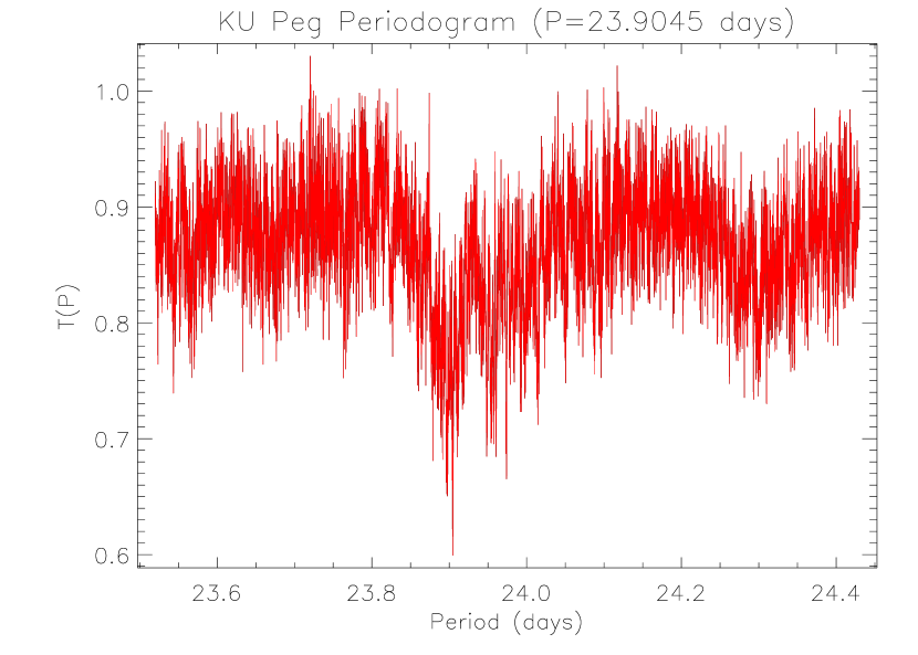
Figure 1: String-length Lafler-Kinman periodogram from APT $V$-band data covering $\approx$18 years. Its best-fit period of 23.9045 d is interpreted to be the rotation period of the star.

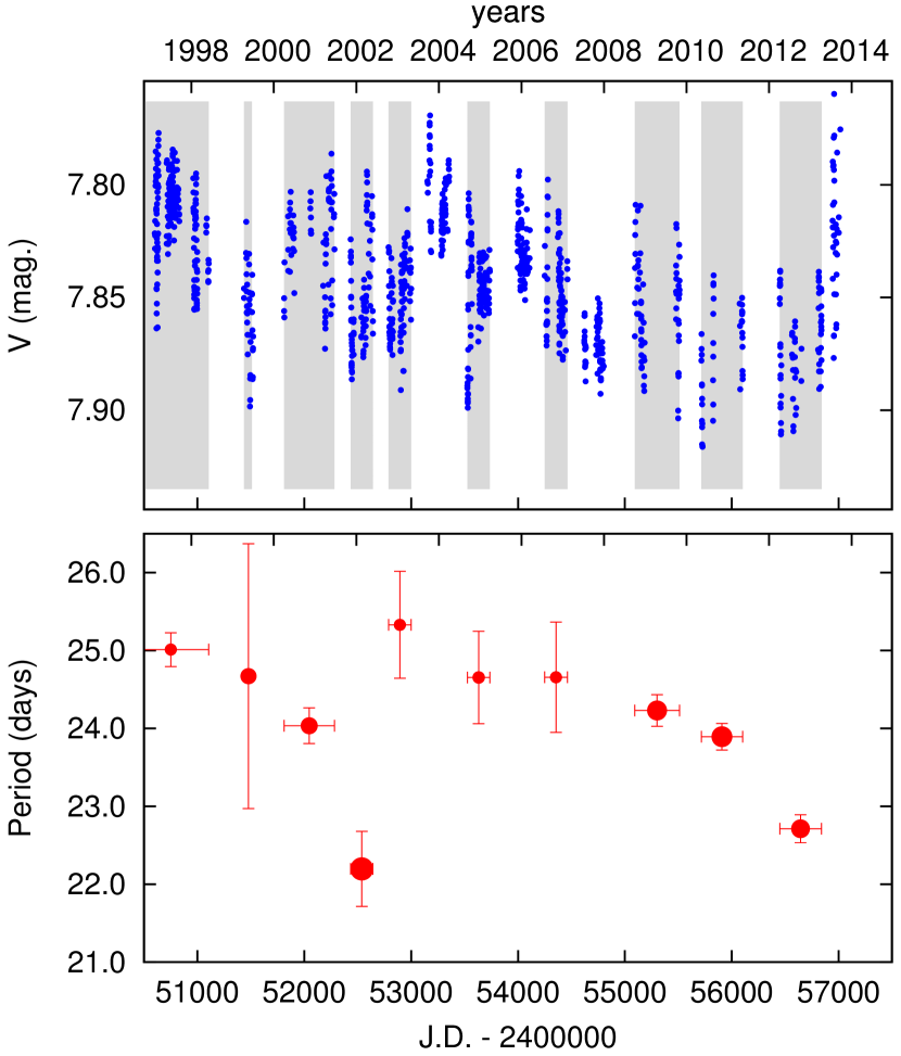
Figure 2: Johnson $V$ observations (top) and seasonally derived photometric periods (bottom) of KU Peg. Each grey band indicates the time range of the data combined for the period determination in the lower panel. In the bottom panel the size of a dot is proportional to the amplitude of the frequency peak in the power spectrum, the vertical error bar represents the uncertainty of the period determination. The horizontal bar just indicates the time coverage.

3 Refinement of the photometric period

Our extended photometric coverage of more than 18 years allows us to derive a more precise rotation period. For the period determination we apply the string-length search using the Lafler-Kinman statistic (hereafter SLLK-method, Clarke 2002). This method phases the light curves with different periods and selects the period giving the smoothest light curve as the correct one. The SLLK-method is particularly useful for finding periods in non-sinusoidal data as compared to standard Fourier analysis. Fig. 1 shows the resulting periodogram and suggests a long-term average photometric period of $P_{\rm phot}=P_{\rm rot}=23.9045\pm 0.0014$ d which we adopt as the best representation of the rotation period of KU Peg. All phase calculations in this paper use this period with the following ephemeris,

$${\rm HJD}=2\,450\,385.5+23.9045\times E,$$ (1)

where the arbitrarily chosen zero point at HJD 2 450 385.5 is taken from Paper I for consistency reasons.

In Paper I a photometric period of $24.96\pm 0.04$ d was derived from the first three years of APT $V$-band data. Its difference of almost one day, i.e. 25$\sigma$, is not only due to measuring errors but due to changing spot locations in combination with differential surface rotation. Photometric periods derived for individual observing seasons on a differentially rotating star are expected to differ from the period from longer-term data (see the review by Strassmeier 2009, and the many references therein). From the range of seasonal periods a rough estimation can be given for the average DR as first introduced by Hall (1972).

In order to determine seasonal periods for KU Peg, we first select adjacent light curves with the criterion that they have similar amplitude, mean brightness, and overall shape. Then, a period is determined for each of these (10) seasonal subsets using our standard Fourier-transformation based frequency analyzer program MuFrAn (Csubry & Kolláth, 2004). Fig. 2 shows the long-term $V$-band APT data along with the subset’s time ranges and the period results. Note that in some cases the light curves were not suitable for deriving a reliable period because of their large scatter compared to the actual amplitude and/or their insufficient length. Table 1 lists the seasonal periods and their errors, which are estimated by increasing the residual scatter of the nonlinear least-squares solutions some degree, which corresponds to 10% of the photometric accuracy (cf. Oláh et al., 2003).

We estimate a DR shear parameter $|\alpha|\gtrsim\Delta P_{\rm phot}/\overline{P}$, where $\Delta P_{\rm phot}$ is the full range of the seasonal period, while $\overline{P}$ is the long-term average. From the values listed in Table 1, we obtain $|\alpha|\gtrsim 0.13\pm 0.05$. This result is similar to the value of +0.09 determined in Paper I from spectroscopy, but considering the errors of either the photometric or the spectroscopic methods, it is also in agreement with the corrected value of +0.03 proposed later by Weber et al. (2005). Note, however, that such a method based simply on photometric data does not allow to determine the sign of the DR parameter $\alpha$ but only the amount of the shear (but see Reinhold & Arlt, 2015).

Table 1: Seasonal periods from our long-term APT photometry.

Seasonal	$P_{\rm phot}$	$\sigma_{P_{\rm phot}}$
mid-HJD	[d]	[d]
2 450 750	25.01	0.22
2 451 478	24.67	1.71
2 452 046	24.04	0.23
2 452 538	22.20	0.48
2 452 894	25.33	0.69
2 453 631	24.66	0.59
2 454 356	24.66	0.71
2 455 302	24.23	0.20
2 455 908	23.89	0.17
2 456 645	22.71	0.18

4 Doppler images for 2006–2011

4.1 Astrophysical parameters of KU Peg

In this section some of the astrophysical parameters are refined with respect to our earlier determinations in Paper I (Weber & Strassmeier, 2001). Among these are the effective temperature ($T_{\rm eff}$), the surface gravity ($\log g$), the metallicity ([Fe/H]), and the projected rotational velocity ($v\sin i$). We employ our SES spectra and the spectrum-synthesis code PARSES (Allende Prieto, 2004; Jovanovic et al., 2013), which is implemented in the standard STELLA-SES data-reduction pipeline (Weber et al., 2008). A grid of synthetic ATLAS-9 spectra tailored to the stellar parameters of KU Peg and for up to 40 échelle orders around 500–750 nm were chosen and the result per spectral order combined on the basis of a weighted least-squares minimization. The average and the standard deviations then constitute our final values and their internal precisions. We found $T_{\rm eff}=4440\pm 10$ K, $\log g$=2.0$\pm$0.1, $v\sin i$=29.4$\pm$1.1  km s^-1  and [Fe/H]=$-0.37\pm 0.02$ with a microturbulence of 1.8 km s^-1 and a prefixed value for the macroturbulence of 3 km s^-1. Note again that the errors are internal errors. External errors are difficult to obtain for spotted stars with broadened line profiles but from past experience we estimate 70 K, 0.2 dex, and 0.1 dex for $T_{\rm eff}$, $\log g$, and [Fe/H], respectively. We note that $T_{\rm eff}$ is lower by 260 K compared to the value of 4700 K in Paper I. However, when taking $(V-I)_{C,{\rm br}}=1\aas@@fstack{m}21\pm 0\aas@@fstack{m}12$ for the brightest (=unspotted) magnitude $V_{\rm br}$ of 7$\aas@@fstack{m}$760$\pm$0.043, observed only just recently (see Fig. 2), a similarly low value of $T_{\rm eff}$ of $4385\pm 20$ K is obtained using the color index vs. temperature calibration by Worthey & Lee 2011. Moreover, taking $B-V=1\aas@@fstack{m}13$ (Strassmeier et al., 2000) together with [Fe/H]=$-0.37$ and using the metallicity-dependent $T_{\rm eff}$-color calibrations by Huang et al. (2015) yields $T_{\rm eff}=4475\pm 83$ K, i.e., again a significantly lower value compared to that in Paper I, but in alignment with the aforementioned determination from $(V-I)_{C}$.

Since this new set of fundamental parameters is in contrast with the ones by previous studies (cf. Lèbre et al., 2009; Aurière et al., 2015) we carried out a comparative study by using the spectrum synthesis code SPECTRUM by R. Gray (www.appstate.edu/$\sim$grayro/spectrum/spectrum.html). We calculated synthetic spectra from our new parameters ($T_{\rm eff}=4440$ K, $\log g$=2.0, $v\sin i$=29.4  km s^-1, [Fe/H]=$-0.37$, and micro- and macroturbulences of $\xi_{\rm mic}$=1.8  km s^-1 and $\xi_{\rm mac}$=3.0  km s^-1, respectively) and from the old parameter set taken from Lèbre et al. (2009), i.e., $T_{\rm eff}=5000$ K, $\log g$=3.0, $v\sin i$=27.1  km s^-1, [Fe/H]=$-0.15$, $\xi_{\rm mic}$=2.0  km s^-1, $\xi_{\rm mac}$=3.0  km s^-1(this latter assumed). The synthetic datasets were compared to the observations (the average of 94 high quality spectra) over the 5950–6510Å spectral range. We found at all times that, in terms of goodness-of-fit values, the synthetic spectra from our new input parameters fitted slightly better the observations. Moreover, the comparisons were extended to some orders between 5000–5600Å, which resulted in similarly better fits for the new parameters, however, with larger rms values due to the ambiguous continuum setting and the increasing line concentration. Accordingly, we beleive that our new fundamental parameters for KU Peg with lower $T_{\rm eff}$ and lower metallicity are more accurate and more consistent. This is strengthened by the color-temperature calibrations from either $B-V$ or $V-I$ measurements, suggesting effective temperatures lower than 5000 K by 250–600 K, depending on the calibration method used (cf. Flower, 1996; Kučinskas et al., 2006; Huang et al., 2015). In addition, our lower metallicity agrees better with the photometric metallicities of $-0.50$ and $-0.39$ determined by Eggen (1993). Finally we note, that most of the spectral type and luminosity classifications of KU Peg in the literature refer to one original determination of G8II by Heard (1956) based on the ‘general appearence’ of objective prism spectra covering much narrower spectral range than ours.

The rotation period from photometry combined with the projected rotational velocity of 29.4$\pm$1.1  km s^-1 from PARSES, and the 50°$\pm$10° inclination angle taken from Paper I, leads to the most likely stellar radius of $R=18.1^{+4.3}_{-2.8}$ R_⊙. For $T_{\rm eff}$ of 4440 K this radius is in good agreement with the expected size of a standard K2III giant star (Dyck et al., 1996). The bolometric magnitude from $R^{2}T_{\rm eff}^{4}$ is then $M_{\rm bol}=-0\aas@@fstack{m}39^{+0.37}_{-0.46}$ (adopting $M_{{\rm bol,}\odot}=4\aas@@fstack{m}74$).

The Hipparcos distance of $202^{+27}_{-22}$ pc (van Leeuwen, 2007) combined with $V_{\rm br}$ and an interstellar extinction of $A_{V}=0\aas@@fstack{m}42$ (cf. Paper I) as well as a bolometric correction of $BC=-0\aas@@fstack{m}64$ from Flower (1996) yields $M_{\rm bol}=0\aas@@fstack{m}17^{+0.30}_{-0.32}$. This value is only insignificantly larger than the value calculated from the radius and the effective temperature. As a tradeoff we take $M_{\rm bol}=-0\aas@@fstack{m}11\pm 0\aas@@fstack{m}28$, i.e., the mean of the two different values, which yields a luminosity of $L=87^{+28}_{-21}L_{\odot}$ for KU Peg.

Fig. 3 shows the position of KU Peg in the Hertzsprung-Russell diagram (HRD) together with stellar evolutionary tracks for $Z$=0.008 of Bertelli et al. (2008). To determine the mass and age of KU Peg, a trilinear interpolation within the three-dimensional space ($L$, $T_{\rm eff}$, [Fe/H]) based on a Monte Carlo method is applied (Künstler et al., 2015). The values obtained are a mass of 1.1 $\pm$ 0.1 $M_{\odot}$ and an age of 7.6 $\pm$ 2.9 Gyr, assuming the metallicity from PARSES. Note, that the mass is about the half of the former value in Paper I, thus increasing the age by a factor of $\approx$9. The refined absolute dimensions and astrophysical quantities summarized in Table 2 are more consistent and with generally smaller error bars when compared to Paper I.

Figure 3: Stellar evolutionary tracks around the RGB bump from Bertelli et al. (2008) for $Z=0.008$ together with the position of KU Peg (dot with error bar). The numbers indicate the corresponding masses in M_⊙. It suggests $M=1.1\pm 0.1M_{\odot}$ as the most likely mass for KU Peg.

Table 2: The astrophysical properties of KU Peg.

Parameter	Value
Spectral type	K2III
DistanceHIP [pc]	$202^{+27}_{-22}$
$V_{\rm br}$ [mag]	$7\aas@@fstack{m}760\pm 0\aas@@fstack{m}043$
$(V-I)_{C,{\rm br}}$ [mag]	$1\aas@@fstack{m}21\pm 0\aas@@fstack{m}12$
$M_{\rm bol}$ [mag]	$-0\aas@@fstack{m}11\pm 0\aas@@fstack{m}28$
Luminosity [$\log\frac{L}{L_{\odot}}$]	$1.94\pm 0.12$
$\log g$ [cgs]	$2.0\pm 0.1$
$T_{\rm eff}$ [K]	$4440\pm 10$
$v\sin i$ [km s-1]	$29.4\pm 1.1$
Rotation period [d]	$23.9045\pm 0.0014$
Inclination [°]	$50\pm 10$
Radius [$R_{\odot}$]	$18.1^{+4.3}_{-2.8}$
Mass [$M_{\odot}$]	$1.1\pm 0.1$
Microturbulence [km s-1]	$1.8\pm 0.1$
Macroturbulence [km s-1]	3.0
Metallicity [Fe/H]	$-0.37\pm 0.02$
NLTE Li abundance (log)	0.1$\pm$0.1

4.2 The STELLA data subsets

The spectroscopic data cover up to three consecutive stellar rotations with fairly good phase sampling in all of the five observing seasons. The detailed time stamps (mid-HJDs) of the data subsets used for the Doppler reconstructions are listed in Table 3. For the 2006 and the 2008 seasons three consecutive data subsets are formed (dubbed S1, S2, and S3, respectively), each covering one single stellar rotation, i.e., one by one suitable for Doppler reconstruction. For the 2009 and 2011 seasons, two consecutive subsets are formed (dubbed S1 and S2, respectively), while for season 2010 only one data set is available.

Table 3: Data subsets for the 11 individual Doppler reconstructions.

Year	Subset	Mid-HJD	Mid-date	Number	Data length	Data length
			[decimal year]	of spectra	[days]	in $P_{\rm rot}$
2006	S1	2 453 959.67	2006.61	19	23.24	0.97
	S2	2 453 980.72	2006.67	20	23.21	0.97
	S3	2 454 013.05	2006.76	21	22.98	0.96
2008	S1	2 454 629.65	2008.45	22	22.92	0.96
	S2	2 454 658.13	2008.52	22	23.82	1.00
	S3	2 454 684.34	2008.60	21	22.95	0.96
2009	S1	2 455 031.29	2009.54	12	22.92	0.96
	S2	2 455 055.46	2009.61	19	21.80	0.91
2010	S1	2 455 448.68	2010.69	12	20.92	0.88
2011	S1	2 455 731.32	2011.46	12	18.96	0.79
	S2	2 455 750.37	2011.52	13	18.87	0.79

4.3 The image reconstruction code iMap

Our DI+ZDI code iMap used in this work performs multi-line inversion for a large number of photospheric line profiles simultaneously (Carroll et al., 2012). Note that in this particular case the DI code is used only. In the case of KU Peg 40 suitable absorption lines, mostly Fe i, were chosen between 5000–6750 Å (Künstler et al., 2015). In the course of the selection, the line depth, the blends, the continuum level, and the temperature sensitivity were taken into consideration.

S1

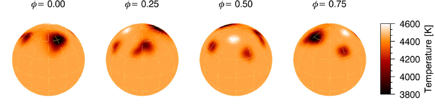
S2

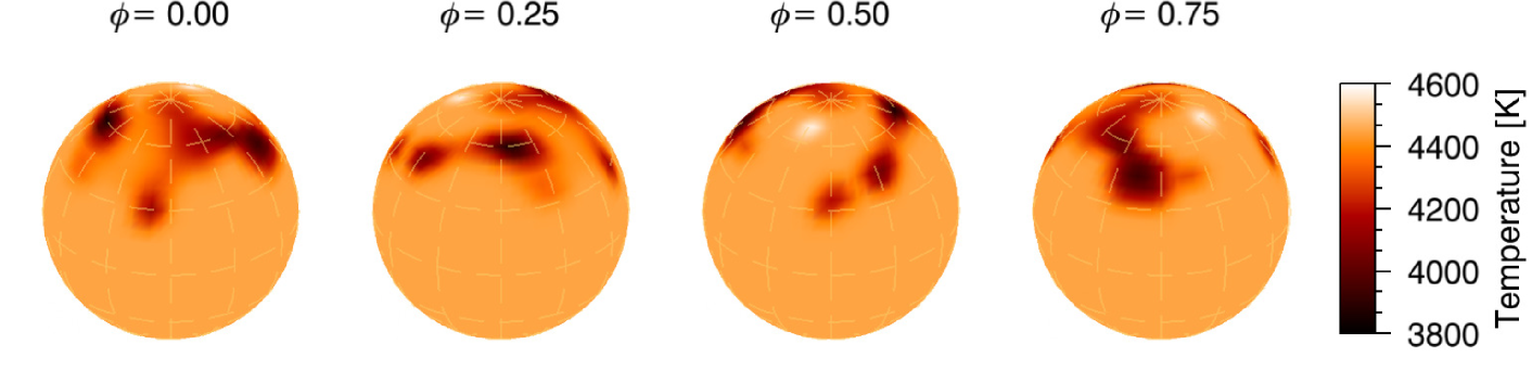
S3

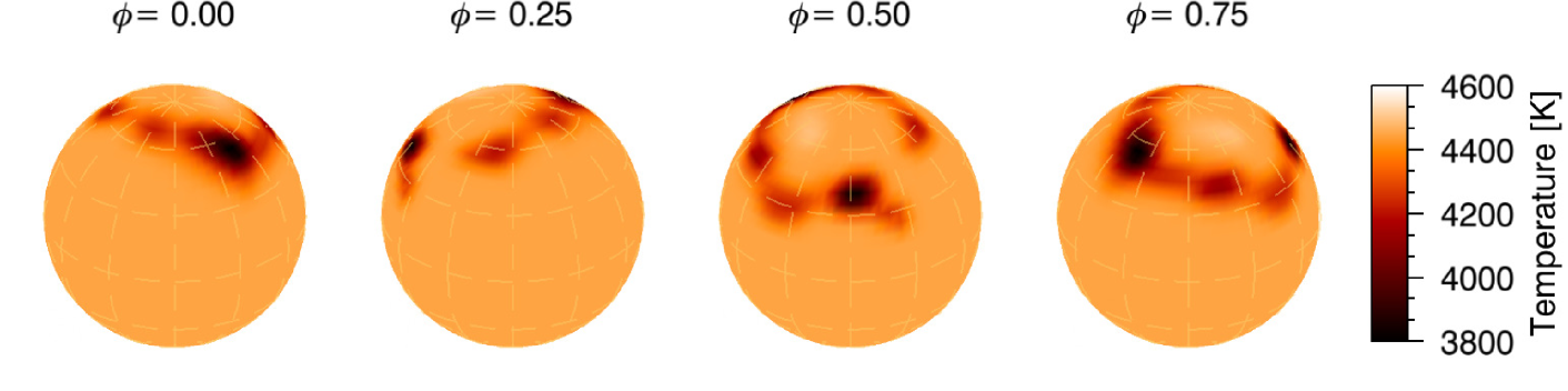
Figure 4: Doppler images of KU Peg for the three data sets S1, S2, and S3 in 2006. The corresponding time stamps in mid-dates are 2006.61, 2006.67, and 2006.76, respectively. The maps are shown in four spherical projections with the corresponding temperature scale. Rotational phase is indicated on the top.

For the line profile calculation iMap solves the radiative transfer using an artificial neural network (Carroll et al., 2008). Individual atomic line parameters are taken from the VALD line database (Kupka et al., 1999). The code uses Kurucz model atmospheres (Castelli & Kurucz, 2004) which are interpolated for each desired temperature, gravity and metallicity. The typical ill-posed nature of the surface inversion is tackled with an iterative regularization based on a Landweber algorithm (Carroll et al., 2012). Therefore, no additional constraints are imposed in the image domain. The surface grid is set to a $5^{\circ}\times 5^{\circ}$ equal-degree partition. For each surface segment the full radiative transfer of all involved line profiles are calculated under the actual effective temperature and atmospheric model. The line profile discrepancy is reduced by adjusting the surface temperature of each segment according to the local temperature gradient information until the minimum $\chi^{2}$ is reached.

S1

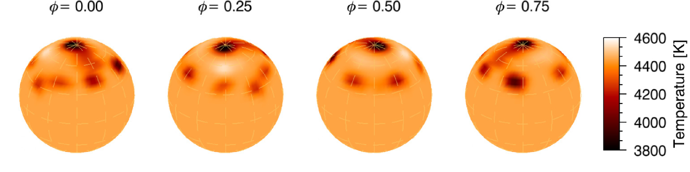
S2

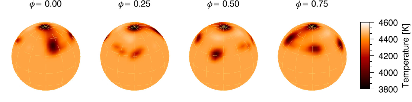
S3

Figure 5: Doppler images of KU Peg for the three data sets S1, S2 and S3 in 2008. The corresponding mid-dates are 2008.45, 2008.52, and 2008.60, respectively. Otherwise as in Fig. 4.

S1

S2

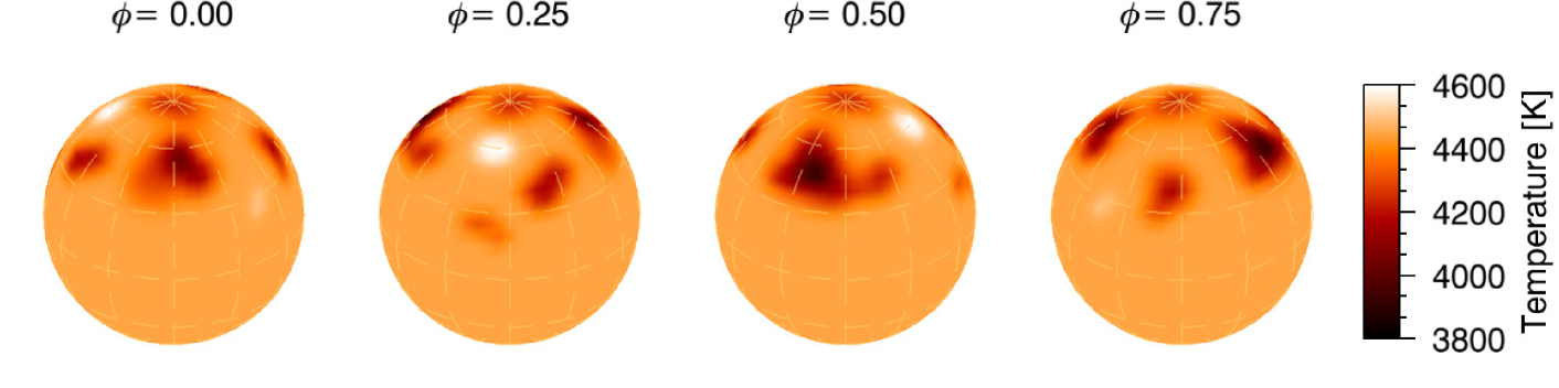
Figure 6: Doppler images of KU Peg for the two datasets S1 and S2 in 2009. The corresponding mid-dates are 2009.54, and 2009.61, respectively. Otherwise as in Fig. 4.

S1

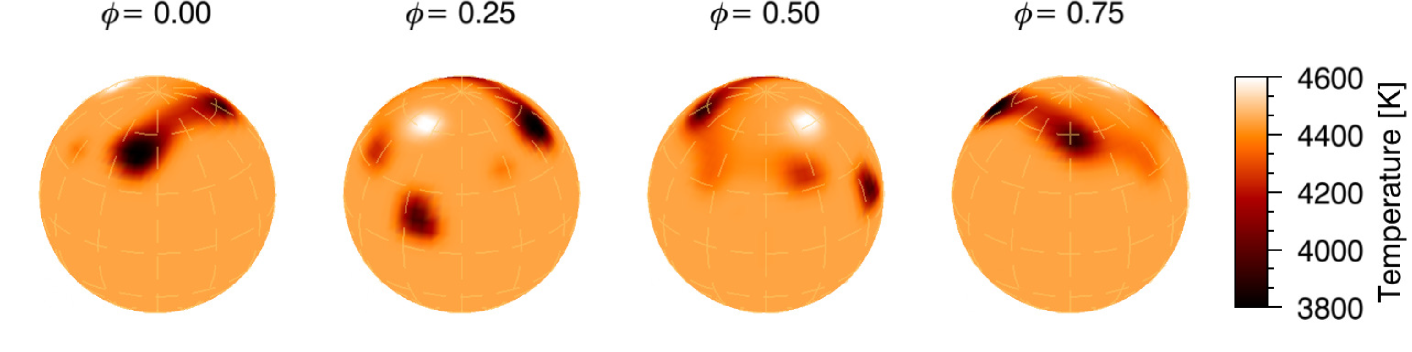
Figure 7: Doppler image of KU Peg for the only available dataset (S1/2010) in 2010. The corresponding mid-date is 2010.69. Otherwise as in Fig. 4.

S1

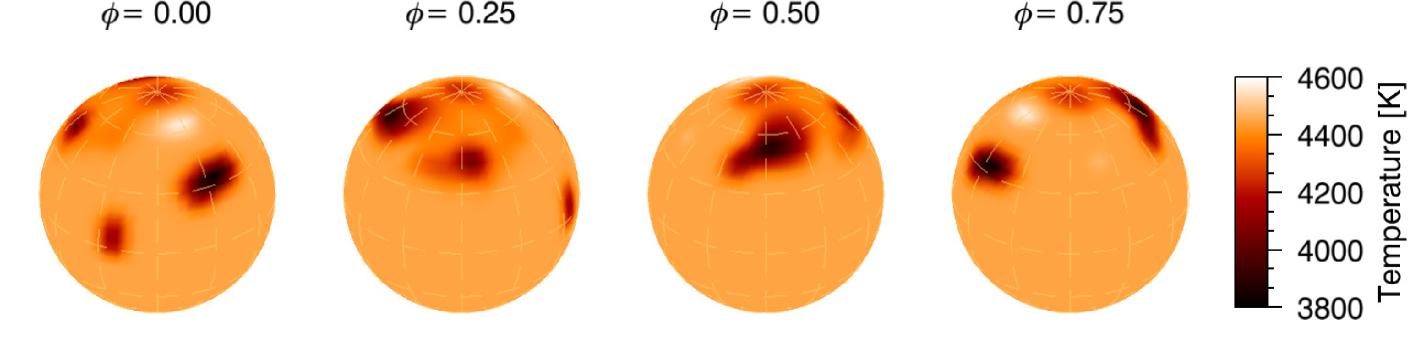
S2

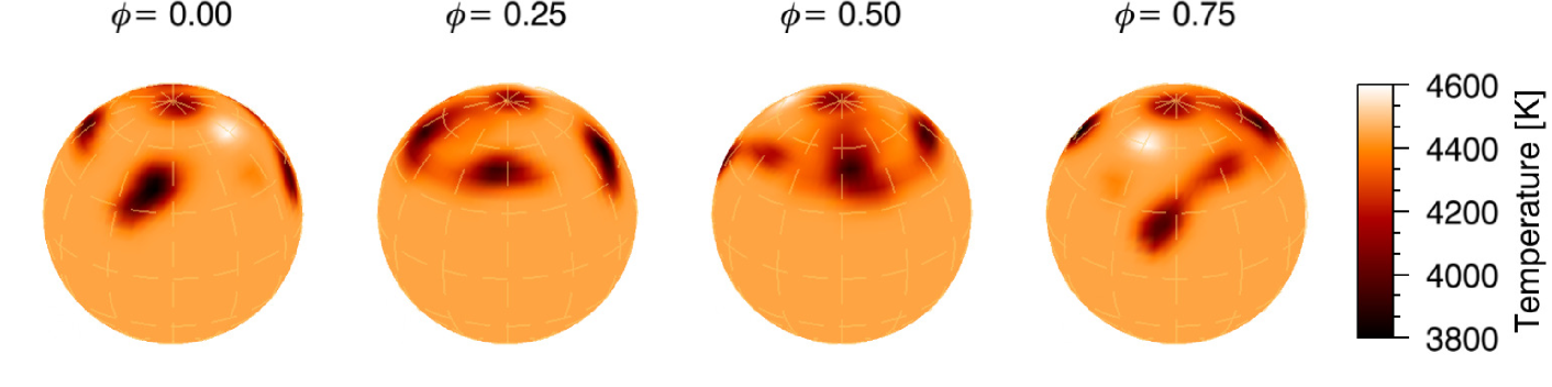
Figure 8: Doppler images of KU Peg for the two available datasets (S1 and S2) in 2011. The corresponding mid-dates are 2011.46 and 2011.52, respectively. Otherwise as in Fig. 4.

4.4 Doppler image reconstructions

Our Doppler reconstructions for KU Peg in Figs. 4–8 reveal spots mostly at mid to high latitudes, sometimes covering the visible pole and sometimes a single spot appears at low latitudes. All in all, the images very much resemble the first Doppler images in Paper I. The temperature of the coolest spots range between $\approx$3650–3850 K, i.e., cooler by $\approx$800 K on average than the photosphere.

The three maps in 2006 (S1, S2 and S3 in Fig. 4) show spots centered at latitudes between 30°–80°. No polar spot is seen. There is also a bright spot at $\phi\approx 0.5$ in S1 with a temperature of $\approx$4700 K, i.e. $\approx$250 K warmer than the surrounding photosphere. This feature appears also in the subsequent independent images but with decreasing size and contrast. The three maps in this mini time-series already indicate the fast time evolution of the spotted surface. Short-term rearrangements are seen throughout, which finally result in a ring-like structure around the visible pole (seen in S3).

In the 2008 season the most prominent feature that appears in all of the three Doppler reconstructions (S1, S2 and S3 in Fig. 5) is the cool polar spot cross talking with another spot centered at around 45° latitude and 15° longitude (i.e., best seen at $\phi=0.0$). Again, there is a bright spot best seen at $\phi=0.25$. However, its contrast is weaker than the feature in 2006 and it almost completely vanishes in the last image of the time series. Most interestingly, a ring-like structure had formed by the end of this mini time series, similar to the one in the map S3/2006.

The most dominant feature in the two consecutive Doppler maps in 2009 (S1 and S2 in Fig. 6) is a cool spot at 50° latitude with a diameter of $\approx$30°. The small polar spot seen a year before is still there but is much weaker. Again there is a small bright spot at 60° latitude (best seen at $\phi=0.25$) which is getting bigger/warmer in the second image. Other, even smaller features are consistently reconstructed in both images and seen to evolve from S1 to S2.

For the one image in 2010 (S1 in Fig. 7) the polar spot had fully disappeared while a high latitude feature with an elongated bipolar structure remained and is now dominating the surface. A bright spot is also seen near 60° latitude but is accompanied by a similar sized cool spot along the same iso-radial line on either side of the central meridian, which makes its reality a little bit suspect. One of its cool counterparts is a rather large and very significant spot though, which is a counterargument because it is actually well constrained.

The two consecutive Doppler images in 2011 (S1 and S2 in Fig. 8) reveal dramatic changes in the spot morphology over just about one stellar rotation. The largest changes are seen at lower latitudes. The one cool spot located at around 45° latitude and 15° longitude in S1 seemed to have been shifted by more than 20° towards increased longitude in S2 or is a product of a merger. The other smaller spot centered at 10° latitude and 345° longitude seems to have either disappeared or merged with the spot at 15° longitude. Meanwhile, a minor displacement of the high latitude bright feature between S1 and S2 is seen in the direction of forward rotation. The most dominant cool spot or spot group in S1 at 180° longitude (best seen at $\phi=0.5$) seems to have started dissolving or at least stretching towards other nearby spots. A weak polar spot seems to be getting stronger in the second map.

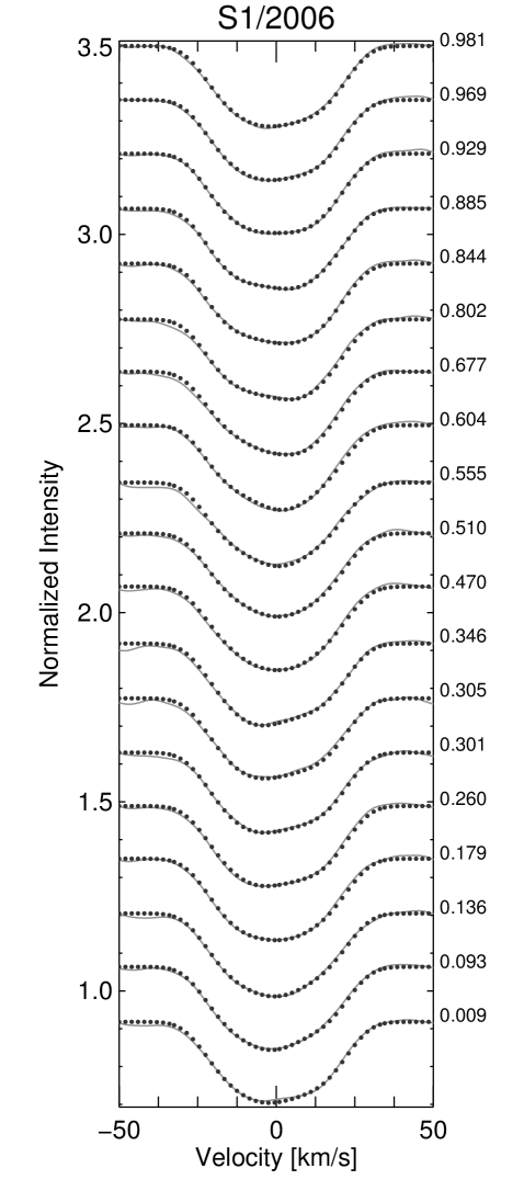
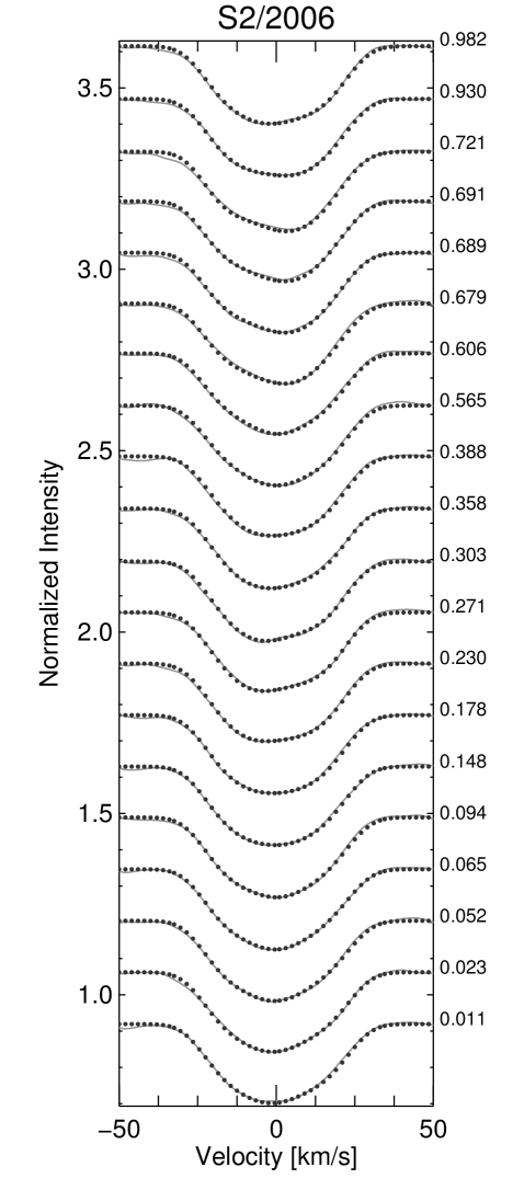
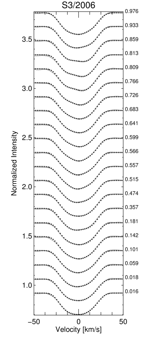
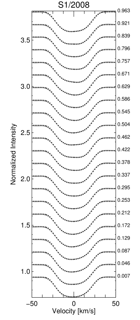
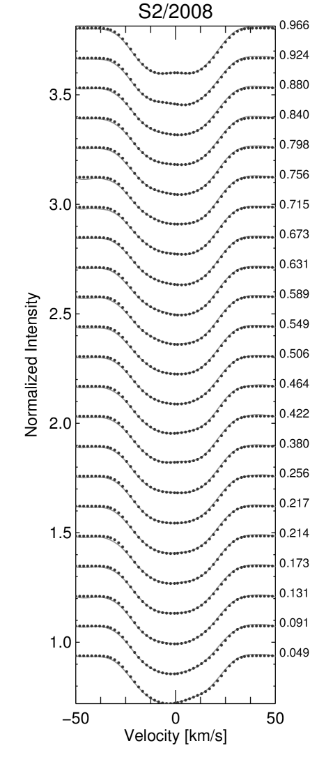
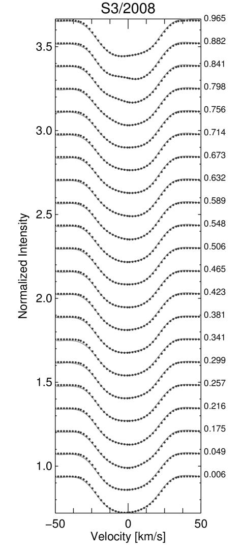
Figure 11: Line profile fits for the Doppler reconstructions shown in Figs. 4–5. The phases of the individual observations are listed on the right side of the panels.

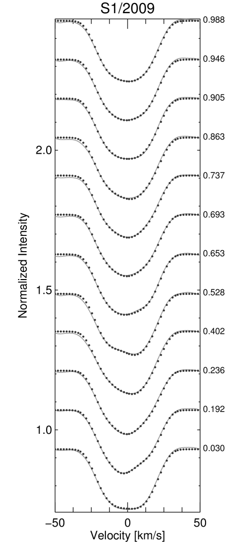
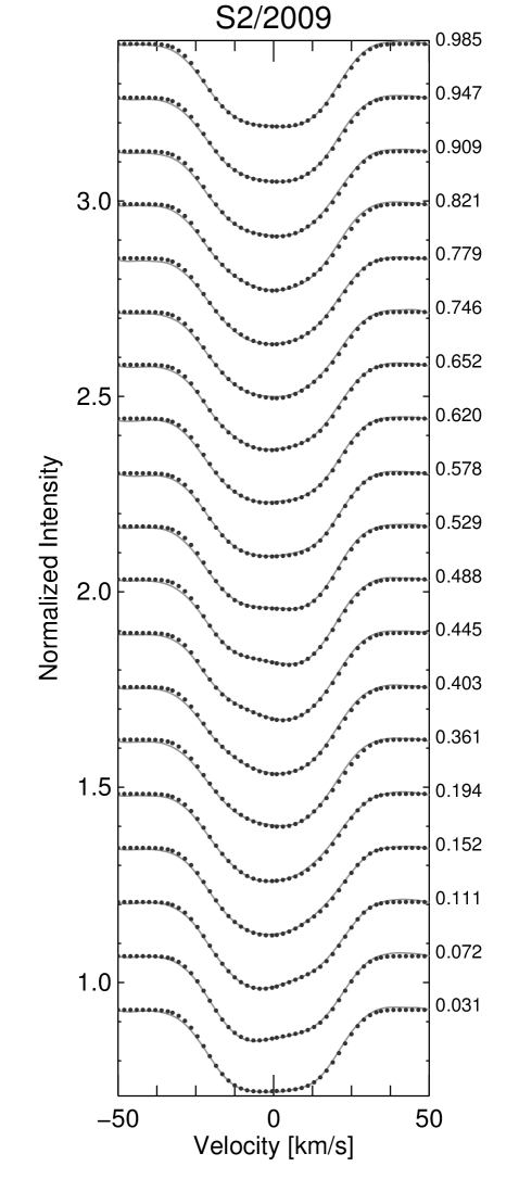
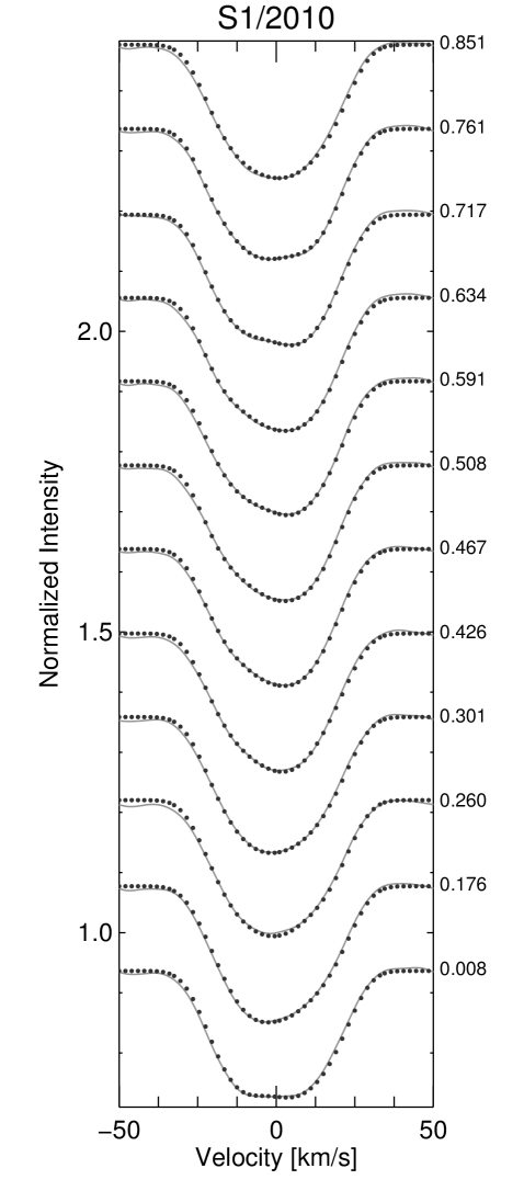
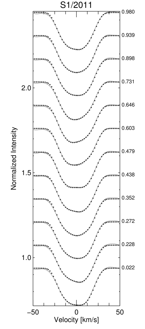
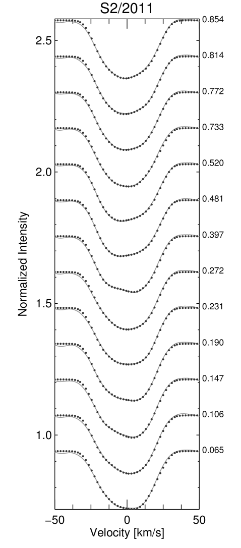
Figure 12: Line profile fits for the Doppler reconstructions shown in Figs. 6–8. The phases of the individual observations are listed on the right side of the panels.

The line profile fits for the altogether 11 Doppler reconstructions in the five observing seasons are plotted in Figs. 11–12 in the Appendix.

5 Surface differential rotation from Doppler images

Time-series Doppler images allow a determination of the surface DR by cross-correlating the consecutive maps with each other. We apply our cross-correlation technique ACCORD (Kővári et al., 2012), which combines all the available surface information in order to achieve an intensified signature of DR. In our case, we have a total of 11 Doppler images. In 2006 and 2008 we have 3 consecutive maps, while in 2009 and 2011 we have 2 consecutive maps. Therefore, we are able to create altogether 8 pairs of maps, i.e., S1-S2, S2-S3 and S1-S3 for 2006 and 2008 and S1-S2 for 2009 and 2011. We cross-correlate the corresponding latitude stripes of the paired Doppler images for each latitude bin of 5°-width, obtaining 8 cross-correlation function maps. These correlation maps are then combined in order to recover an average correlation pattern from which we determine the surface DR. For a more detailed description of the ACCORD technique we refer to our recent application in Kővári et al. (2015) and the references therein.

Fig. 9 shows the average correlation pattern with the best-fit quadratic rotation law. Note that due to the limited appearance of spots at low latitudes, the weak correlation pattern at latitudes below $\approx$ 40° must be rejected. Yet the dashed-line function clearly represents a solar-type DR. The rotation law in the usual quadratic form takes the shape $\Omega(\beta)=\Omega_{\rm eq}(1-\alpha\sin^{2}\beta)$, where $\Omega(\beta)$ is the angular velocity at $\beta$ latitude, $\Omega_{\rm eq}$ is the equatorial angular velocity, while $\alpha=\Delta\Omega/\Omega_{\rm eq}$ is the surface shear coefficient and $\Delta\Omega=\Omega_{\rm eq}-\Omega_{\rm pol}$ is the angular velocity difference between the equator and the pole. The best fit yields $\Omega_{\rm eq}=15.5138$°/d (or equivalently $P_{\rm eq}=23.2051$ d) and $\alpha=+0.040\pm 0.006$. This can be converted to a lap time of $\approx$580 d, i.e., the time needed by the equator to lap the polar regions. This result is in the order of the empirical estimation of $|\alpha|\approx P_{\rm rot}/360\,{\rm d}$ deduced by Kővári & Oláh (2014) from Doppler imaging studies of either single stars or members of binary systems. Note however, that the statistically small sample of comparably fast rotating single giants with known surface DR does not allow to give such a relationship for single giants only.

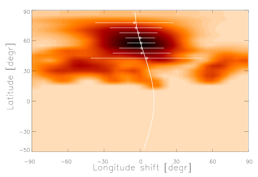
Figure 9: Average cross-correlation function map showing the evidence for surface differential rotation. Darker shade represents better correlation. The average longitudinal cross-correlation functions in 5° bins are fitted by Gaussian curves. Gaussian peaks are indicated by dots, the corresponding Gaussian widths by horizontal lines. The continuous line is the best fit, suggesting solar-type differential rotation with $P_{\rm eq}=23.2051$ d equatorial period and $\alpha=+0.040$ surface shear.

6 Li abundance determination

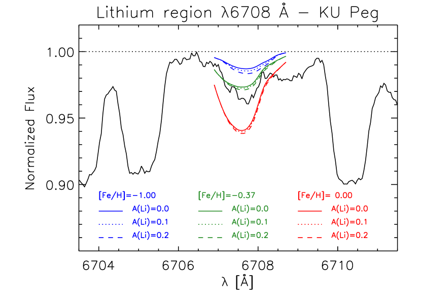
Figure 10: Li i 6708 Å spectral region of KU Peg. The observed spectrum is an average of 40 individual exposures taken in July/Aug 2009. The three sets of thin lines are synthetic spectra for three metallicities (see insert, for –1.00, –0.37 and 0.0) and for three Li abundances of $\log n$=0.0, 0.1, and 0.2. Our best estimate with a metallicity of –0.37 suggests an upper Li limit of $\log n$=0.1$\pm$0.1.

In Fig. 10 the extracted spectral region around the Li i-6708 Å line is plotted. Visual inspection of individual exposures does not show any striking evidence of a Li i-6708 Å line, hampered by the large $v\sin i$ (30  km s^-1) and the comparably low S/N (on average 100:1 for a single exposure). Only after co-adding 40 spectra from within two months in 2009 (July/Aug) a consistent asymmetry of the Fe i and CN blends appears. However, the averaging smears the line profile shapes due to the rotationally modulated spot contribution and makes the average line strength appear weaker than it is. This may be a few-% effect in the equivalent width but we believe it can be neglected because the uncertainty of the continuum setting is so much larger. A straight-forward double Gaussian fit to the average spectrum centered at the average Li i-6708 Å line wavelength and the Fe i-6707.43 blend results in a mere $\approx$5 mÅ Li equivalent width. It converts to a logarithmic abundance of $\approx$0.1$\pm$0.1 relative to hydrogen ($\log n$(H)=12.00) with the NLTE tables of Pavlenko & Magazzu (1996); if it is all due to Li and for the case that the models are error free. Such a low Li abundance is not seen on other rapidly-rotating K giants of comparable luminosity and KU Peg may be an interesting target also for constraining the Li dredge-up problem.

We also compare our average spectrum with a small grid of forward synthetic Li spectra from 3D model atmospheres. A formal fit of the spectrum was not possible with the current set-up due to the lack of the appropriate 3D models and the comparable large $v\sin i$ and low S/N of the data. However, Fig. 10 compares three sets of synthetic spectra for metallicities of between solar and ten times less than solar and with logarithmic Li abundances of $A$(Li)=0.0, 0.1, and 0.2, i.e., approximately ten times below the solar value ($\log n_{\odot}$=1.05$\pm$0.1; Asplund et al. 2009). We note that changing the continuum of the observed spectrum by just 1% has already a 0.2-dex impact on the Li abundance and similar is the case for the metallicity. Nevertheless, the 3D synthetic spectra agree with the equivalent width above and constrain the Li abundance to an upper limit of $\log n$=0.1$\pm$0.2. Its uncertainty is estimated from the case when the metallicity and the continuum location are assumed to be free of error. We adopted the new line list given in Caffau et al. (2015) with a total of 40 spectral lines plus the hyperfine structure of the Li resonance. Line computations were done from 3D CO5BOLD model atmospheres matching the temperature and gravity of KU Peg in Table 2.

7 Summary and discussions

Our new Doppler image reconstructions of KU Peg indicate that its surface spot distribution is indeed very active and dynamic, even when compared to other overactive stars, and so must be the underlying dynamo. According to the theoretical estimation by Aurière et al. (2015) the maximum convective turnover time of KU Peg should be around $\tau\approx 100$ d. This would yield a moderate Rossby number of $Ro\approx 0.24$, indicating that the star operates an $\alpha\Omega$ type dynamo. However, from the time evolution of the spotted surface, considering especially the polar spottedness between 2006-2011, we could only estimate a rough cycle length of a few years. On the other hand, from long-term photometry, such a cycle (of about 2–4 years) can be inferred at a very weak significance level, i.e., not conclusively.

From our cross-correlation study, we derived a solar-like surface DR with a shear of $\alpha=+0.040\pm 0.006$ and a lap time of $\approx$580 days. A similar solar-like DR was found in Paper I with $\alpha=+0.09$ and a corresponding lap time of $\approx$260 days. Note that the higher value in Paper I came from a cross-correlation of only two consecutive Doppler maps and the use of a less-robust correlation routine which both resulted in a less pronounced correlation pattern. A redetermination of $\alpha$ with a different cross-correlation program but the same data as in Paper I by Weber et al. (2005), revealed an $\alpha$ of +0.03, in agreement with our new value. In the present paper, we applied a more robust cross-correlation technique for altogether 8 cross-correlation maps and conclude that our new result is much more reliable and has now a reasonable error bar.

The time-series Doppler reconstructions revealed evidence for systematic spot displacements that may be interpreted as evidence for local meridional flows. Examples are the poleward drift of the dominant feature in Fig. 4 at $\phi=0.25$ or the displacement of the low latitude spot in Fig. 6 at $\phi=0.25$ (as well as in Fig. 8 at $\phi=0.00$ and at $\phi=0.25$). Compared to the longitudinal displacements due to DR, the latitudinal displacements are more diffused and much weaker on average. At the same time the overall evolution of the spot distribution is generally more complex than thought and can have spots come and go from one rotation to the next (e.g. in 2011, Fig. 8).

Rapid rotation of an old, effectively single, evolved star like KU Peg remains a challenge for theory. If tidal effects did not play a role in the past of the star, the most likely explanation for its rapid rotation would be that a deepening convective envelope eventually reaches the high angular momentum material around a fast rotating core, and thus transports high angular momentum material up to the surface on a comparably short convective time scale (Endal & Sofia, 1979). This dredge up must take place before the star evolves up to the bump of the red giant branch. On the other hand, with the expanding envelope an increasing mass loss rate would be expected, which would again mean angular momentum loss. However, excessive mass loss can be excluded by the lack of any IR excess from a comparison of the measured (2MASS) $J$, $H$ and $K$ magnitudes and the color calibrations provided by Ramírez & Meléndez (2005). But out-flowing material can also be coupled to closed surface magnetic fields, generated by a dynamo, this way preventing the star from fast angular momentum loss (cf. Cohen et al., 2010).

In any case, a rapidly rotating core on the main sequence is required to explain the spin-up by angular momentum transport from the deep. However, it is not likely that a star of $1.1\,M_{\odot}$ could provide such a fast rotating core. Moreover, according to Privitera et al. (2016a) the dredge up may not produce enough acceleration of the surface to be a reasonable explanation at all.

As an alternative scenario, engulfment of one planet (or even more) may explain the rapid rotation (Siess & Livio, 1999; Carlberg et al., 2012; Privitera et al., 2016b). Taken the expression from Massarotti et al. (2008) we estimate the mass of the planet which would spin up the star to be $\approx$1.25 $M_{\rm J}$. But this would also raise the Li abundance at the surface rather than lowering it, which is found for KU Peg. Note however, that according to Casey et al. (2016) any close giant planet is likely to be engulfed well before the host star would evolve up the RGB. This would explain the low surface Li abundance, since by the end of the dredge up phase the extra Li coming from the planet will be destroyed together with the primeval Li of the stellar envelope. But anyhow, lithium can be affected by other less known processes too, thus the surface Li measurement itself can hardly account for or disprove any planetary interaction as pointed out by Privitera et al. (2016b).

The position in the H-R diagram indicates that KU Peg is past the RGB luminosity bump. Only low-mass stars that have a highly degenerate He core on the RGB, and later undergo the He flash, evolve through this phase (see Charbonnel & Balachandran, 2000). At this time extra Li is produced and very high Li abundances are reached (e.g., HD 233517; Strassmeier et al., 2015). However, this phase is extremely short lived because once the mixing extends deep enough the freshly synthesized Li is quickly destroyed. Immediately before the bump phase (and after the end of the first dredge-up), we expect relatively low Li abundances. The time-scale of the bump for $M=1.1\mathrm{M}_{\sun}$ and $Z$=0.008 (almost equivalent with [Fe/H]=$-$0.37) is $\approx$10 Myr, the time between the bump and the current position of KU Peg is $\approx$40 Myr according to the models of Bertelli et al. (2008). This must have been enough time to dilute KU Peg’s surface Li to basically zero.

Appendix A Observing log and line profile fits

Table 4: Observing log of STELLA-I SES spectra taken between 2006–2011.

HJD	Phase	S/N	Subset/year	HJD	Phase	S/N	Subset/year	HJD	Phase	S/N	Subset/year
3947.4901	0.009	40	S1/2006	4623.6530	0.295	117	S1/2008	5028.6074	0.236	122	S1/2009
3949.4836	0.093	40	S1/2006	4624.6476	0.337	127	S1/2008	5032.5866	0.402	120	S1/2009
3950.5241	0.136	35	S1/2006	4625.6432	0.378	133	S1/2008	5035.6056	0.528	80	S1/2009
3951.5597	0.179	46	S1/2006	4626.6788	0.422	139	S1/2008	5038.5754	0.653	77	S1/2009
3953.4742	0.260	38	S1/2006	4627.6493	0.462	114	S1/2008	5039.5280	0.693	120	S1/2009
3954.4723	0.301	25	S1/2006	4628.6382	0.504	136	S1/2008	5040.5974	0.737	139	S1/2009
3954.5571	0.305	22	S1/2006	4629.6326	0.545	103	S1/2008	5043.6119	0.863	105	S1/2009
3955.5405	0.346	27	S1/2006	4630.6139	0.586	98	S1/2008	5044.6923	0.909	76	S2/2009
3958.5047	0.470	52	S1/2006	4631.6384	0.629	120	S1/2008	5045.6145	0.947	85	S2/2009
3959.4636	0.510	56	S1/2006	4632.6346	0.671	137	S1/2008	5046.5245	0.985	122	S2/2009
3960.5446	0.555	24	S1/2006	4634.6920	0.757	107	S1/2008	5047.6092	0.031	144	S2/2009
3961.7125	0.604	41	S1/2006	4635.6335	0.796	120	S1/2008	5048.6052	0.072	145	S2/2009
3963.4532	0.677	36	S1/2006	4636.6556	0.839	115	S1/2008	5049.5334	0.111	126	S2/2009
3966.4524	0.802	26	S1/2006	4638.6139	0.921	82	S1/2008	5050.5126	0.152	116	S2/2009
3967.4415	0.844	35	S1/2006	4639.6265	0.963	117	S1/2008	5051.5125	0.194	126	S2/2009
3968.4339	0.885	37	S1/2006	4640.6610	0.007	112	S1/2008	5055.5099	0.361	135	S2/2009
3969.4851	0.929	57	S1/2006	4641.5962	0.046	101	S1/2008	5056.5084	0.403	115	S2/2009
3970.4301	0.969	48	S1/2006	4645.6956	0.217	100	S2/2008	5057.5084	0.445	141	S2/2009
3970.7259	0.981	58	S1/2006	4646.6213	0.256	94	S2/2008	5058.5318	0.488	135	S2/2009
3971.4292	0.011	34	S2/2006	4649.5961	0.380	100	S2/2008	5059.5327	0.529	129	S2/2009
3971.7251	0.023	37	S2/2006	4650.5906	0.422	114	S2/2008	5060.7000	0.578	80	S2/2009
3972.4294	0.052	40	S2/2006	4651.5976	0.464	128	S2/2008	5061.6971	0.620	134	S2/2009
3972.7261	0.065	42	S2/2006	4652.5943	0.506	112	S2/2008	5062.4696	0.652	125	S2/2009
3973.4273	0.094	43	S2/2006	4653.6199	0.549	116	S2/2008	5064.7071	0.746	85	S2/2009
3974.7180	0.148	42	S2/2006	4654.5914	0.589	96	S2/2008	5065.5002	0.779	71	S2/2009
3975.4258	0.178	52	S2/2006	4655.5802	0.631	91	S2/2008	5066.4959	0.821	130	S2/2009
3976.6662	0.230	45	S2/2006	4656.5973	0.673	91	S2/2008	5439.5302	0.426	86	S1/2010
3977.6598	0.271	45	S2/2006	4657.5933	0.715	100	S2/2008	5440.5185	0.467	123	S1/2010
3978.4228	0.303	44	S2/2006	4658.5764	0.756	103	S2/2008	5441.4937	0.508	123	S1/2010
3979.7216	0.358	44	S2/2006	4659.5886	0.798	130	S2/2008	5443.4856	0.591	106	S1/2010
3980.4605	0.388	50	S2/2006	4660.5857	0.840	125	S2/2008	5444.5140	0.634	112	S1/2010
3984.6764	0.565	48	S2/2006	4661.5311	0.880	121	S2/2008	5446.4904	0.717	72	S1/2010
3985.6648	0.606	51	S2/2006	4662.5817	0.924	103	S2/2008	5447.5329	0.761	91	S1/2010
3987.4155	0.679	59	S2/2006	4663.5849	0.966	115	S2/2008	5449.6861	0.851	110	S1/2010
3987.6347	0.689	53	S2/2006	4665.5716	0.049	122	S2/2008	5453.4555	0.008	64	S1/2010
3987.6892	0.691	54	S2/2006	4666.5779	0.091	118	S2/2008	5457.4696	0.176	116	S1/2010
3988.4145	0.721	55	S2/2006	4667.5328	0.131	81	S2/2008	5459.4770	0.260	69	S1/2010
3993.4111	0.930	65	S2/2006	4668.5316	0.173	104	S2/2008	5460.4521	0.301	112	S1/2010
3994.6385	0.982	63	S2/2006	4669.5129	0.214	105	S2/2008	5721.6610	0.228	124	S1/2011
3999.4056	0.181	65	S3/2006	4673.5035	0.381	99	S3/2008	5722.6971	0.272	146	S1/2011
4003.6096	0.357	86	S3/2006	4674.5176	0.423	106	S3/2008	5724.6215	0.352	116	S1/2011
4006.4000	0.474	78	S3/2006	4675.5124	0.465	95	S3/2008	5726.6656	0.438	95	S1/2011
4007.3988	0.515	71	S3/2006	4676.5012	0.506	122	S3/2008	5727.6438	0.479	112	S1/2011
4008.3963	0.557	49	S3/2006	4677.5089	0.548	109	S3/2008	5730.6297	0.603	141	S1/2011
4008.6148	0.566	48	S3/2006	4678.4906	0.589	97	S3/2008	5731.6411	0.646	93	S1/2011
4009.3968	0.599	75	S3/2006	4679.5136	0.632	95	S3/2008	5733.6768	0.731	107	S1/2011
4010.3972	0.641	70	S3/2006	4680.4960	0.673	98	S3/2008	5737.6814	0.898	133	S1/2011
4011.3954	0.683	70	S3/2006	4681.4788	0.714	105	S3/2008	5738.6419	0.939	99	S1/2011
4012.4237	0.726	52	S3/2006	4682.4761	0.756	114	S3/2008	5739.6380	0.980	73	S1/2011
4013.3943	0.766	56	S3/2006	4683.4900	0.798	110	S3/2008	5740.6246	0.022	115	S1/2011
4014.4257	0.809	35	S3/2006	4684.5041	0.841	105	S3/2008	5741.6552	0.065	95	S2/2011
4014.5202	0.813	35	S3/2006	4685.4908	0.882	85	S3/2008	5742.6304	0.106	112	S2/2011
4015.6057	0.859	67	S3/2006	4687.4826	0.965	95	S3/2008	5743.6332	0.147	84	S2/2011
4017.3877	0.933	68	S3/2006	4688.4611	0.006	111	S3/2008	5744.6525	0.190	73	S2/2011
4018.4017	0.976	64	S3/2006	4689.4824	0.049	118	S3/2008	5745.6220	0.231	107	S2/2011
4019.3718	0.016	33	S3/2006	4692.4841	0.175	98	S3/2008	5746.6009	0.272	108	S2/2011
4019.4138	0.018	47	S3/2006	4693.4718	0.216	75	S3/2008	5749.5862	0.397	108	S2/2011
4020.3879	0.059	73	S3/2006	4694.4601	0.257	103	S3/2008	5751.6024	0.481	147	S2/2011
4021.3878	0.101	82	S3/2006	4695.4523	0.299	117	S3/2008	5752.5473	0.520	134	S2/2011
4022.3871	0.142	61	S3/2006	4696.4539	0.341	94	S3/2008	5757.6309	0.733	134	S2/2011
4618.6745	0.087	130	S1/2008	5020.6934	0.905	123	S1/2009	5758.5582	0.772	92	S2/2011
4619.6683	0.129	98	S1/2008	5021.6844	0.946	145	S1/2009	5759.5616	0.814	85	S2/2011
4620.6966	0.172	127	S1/2008	5022.6944	0.988	103	S1/2009	5760.5258	0.854	127	S2/2011
4621.6611	0.212	114	S1/2008	5023.6911	0.030	118	S1/2009
4622.6505	0.253	136	S1/2008	5027.5709	0.192	135	S1/2009