Work fluctuation and total entropy production in nonequilibrium processes

Abstract

Work fluctuation and total entropy production play crucial roles in small thermodynamic systems subject to large thermal fluctuations. We investigate a trade-off relation between them in a nonequilibrium situation in which a system starts from an arbitrary nonequilibrium state. We apply the variational method to study this problem and find a stationary solution against variations over protocols that describe the time dependence of the Hamiltonian of the system. Using the stationary solution, we find the minimum of the total entropy production for a given amount of work fluctuation. An explicit protocol that achieves this is constructed from an adiabatic process followed by a quasi-static process. The obtained results suggest how one can control the nonequilibrium dynamics of the system while suppressing its work fluctuation and total entropy production.

I Introduction

Recent developments in thermodynamics of small systems based on information theoretic concepts allow one to formulate the second law of thermodynamics for arbitrary nonequilibrium initial and final states and under measurement and feedback control Parrondo ; Hasegawa ; Takara ; Esposito2 ; Deffner . By using nonequilibrium free energies Esposito2 ; Deffner , we can quantify the extractable work from information heat engines Maxwell ; Maruyama ; Sagawa2 ; JMaxwell ; Szilard ; Horowitz3 ; Sagawa4 , the thermodynamic cost of information erasure Landauer ; Rio and that of a nonequilibrium thermodynamic task Esposito2 in a unified manner. Applications of fluctuation theorems Jarzynski1 ; Jarzynski2 ; Crooks ; Esposito ; fluctuation1 and stochastic thermodynamics Sekimoto ; Seifert to these general nonequilibrium situations have been made and they provide a method to construct a protocol that reduces the entropy production during nonequilibrium processes Hasegawa ; Esposito2 .

Experimental advances, on the other hand, allow us to manipulate the microscopic degrees of freedom of small fluctuating systems. The Szilard engine and Landauer’s information erasure have been demonstrated using a single-electron box Koski1 ; Koski2 and a colloidal particle Toyabe ; Berut ; colloidal ; John . Because the amount of work fluctuation is not negligible in mesoscopic and nano systems, much effort has been devoted to suppress excitations and work fluctuation during the nonequilibrium dynamics, thereby allowing us to obtain a faster convergence of the Jarzynski equality and an increase in the output power of heat engines STA1 ; STA2 ; Wfluc1 . Meanwhile, the study of single-shot statistical mechanics has attracted much attention recently which applies the one-shot information theory Renner to thermodynamics, thereby extracting useful information on the work from a single trial of the experiment Aberg ; Horodecki ; Fernando1 ; Fernando2 ; Lostaglio ; Salek ; Horodecki2 ; Oscar1 ; Oscar . In particular, a protocol with vanishing work fluctuation (deterministic work extraction protocol) Aberg ; Horodecki and the upper bound of the unaveraged work cost (worst-case work) Oscar1 ; Oscar have been studied. The bounds on the work cost that can be derived from the deterministic work extraction protocol Aberg ; Horodecki give severe constraints on the work compared with those of the conventional second law of thermodynamics. The basic settings to derive fluctuation theorems and the deterministic work extraction protocol are different in general, and several studies discuss the link between them Aberg ; Oscar ; Salek ; Funo . In Ref. Funo , two of the present authors discuss a protocol which reduces both work fluctuation and total entropy production as much as possible in small thermodynamic systems. However, an implicit assumption made in that paper to derive the work fluctuation-dissipation trade-off relation turns out to be valid only for some specific range of the initial states as detailed in Appendix B. Recently, the stochastic uncertainty relation which relates the fluctuation in a current and the dissipation rate has been investigated UC1 ; UC2 ; UC3 . Deriving some trade-off relations between fluctuation and dissipation in various nonequilibrium situations should attract considerable interest in stochastic thermodynamics.

In this paper, we remove the assumption made in Ref. Funo and derive a rigorous trade-off relation between the work fluctuation and the total entropy production in nonequilibrium processes for arbitrary initial states. We derive the minimum of the total entropy production for a given work fluctuation. An explicit protocol that achieves the minimum total entropy production is presented, giving us an efficient way of transforming a nonequilibrium state into a thermalized state by suppressing both work fluctuation and total entropy production as much as possible. The thermodynamically reversible protocol is reproduced in the limit of vanishing total entropy production. We derive the detailed fluctuation theorem for the single-shot setting, and show that the deterministic work extraction protocol is obtained in the limit of vanishing work fluctuation.

This paper is organized as follows. In Sec. II, we describe the system discussed in this paper and the assumptions made to derive the main results. In Sec. III, we apply the variational method to obtain the stationary solution. An explicit protocol that gives the stationary solution is given. In Sec. IV, we derive the minimum of the total entropy production for a given work fluctuation by using the obtained stationary solution, which is the main result of this paper. In Sec. V, we take the limit of vanishing total entropy production and that of vanishing work fluctuation, and show that the deterministic work extraction protocol and the thermodynamically reversible protocol are reproduced. We summarize the main results of this paper in Sec. VI. In Appendix A, we derive the detailed fluctuation theorem for the dynamics of the system described by the thermal operation, and derive the deterministic work extraction protocol on the basis of the detailed fluctuation theorem. In Appendix B, we compare our main results with those obtained in Ref. Funo . In particular, we discuss a class of initial states such that the trade-off relation derived in Ref. Funo gives numerical values close to those obtained in this paper.

II Setup

We consider a situation in which the Hamiltonian of the system is externally driven according to a protocol $\lambda_{i}:=\lambda(t_{i})$ and consider discrete times $t\in\{t_{0},t_{1},\cdots,t_{N}\}$. We note that once we specify a protocol $\{\lambda_{i}\}$, the Hamiltonian of the system $H_{\lambda_{i}}$ and thus the energy eigenvalues $\{E_{\lambda_{i}}(y_{i})\}$ are specified for the entire process. Here, we assume that the system interacts with a single heat bath whose inverse temperature is $\beta$. Suppose that the initial and final Hamiltonians ($H_{\lambda_{0}}$ and $H_{\lambda_{N}}$) are fixed, and that the initial and final states are given by $p_{\mathrm{ini}}(x_{0})$ and $p^{\mathrm{can}}_{\lambda_{N}}(x_{N})$, respectively. Here, the initial state is an arbitrary nonequilibrium distribution but the final state is assumed to be given by the canonical distribution, to disregard the nonequilibriumness of the final state which leads to a reduction in the extractable work. By this assumption, we focus on the effect of the nonequilibriumness of the initial state and discuss the optimal extractable work (which is equivalent to the minimal total entropy production as can be checked by comparing Eqs. (11) and (12) below) for a given work fluctuation. We assume that the dynamics of the system satisfies the detailed fluctuation theorem Crooks in Eq. (10). It can be derived for the classical stochastic dynamics Seifert , isolated quantum systems Tasaki ; Kurchan and open quantum systems Horowitz1 ; Horowitz2 ; Hekking ; Liu1 . For quantum systems, we assume that the initial state does not have coherence between energy eigenstates.

II.1 Classical stochastic dynamics

We first consider a classical Markovian dynamics described by the master equation. We consider a discrete time evolution and denote the discretized trajectory of the system as $\Gamma=\{x_{0},x_{1},\cdots,x_{N}\}$, where $x_{i}$’s denote the configuration points of the system at time $t_{i}$. Then, the system evolves in time according to the following master equation:

$$p(x_{i+1})=\sum_{x_{i}}p(x_{i})p(x_{i}\rightarrow x_{i+1}|H_{\lambda_{i+1}}),$$ (1)

where $p(x_{i})$ is the probability of the system being found at $x_{i}$ and $p(x_{i}\rightarrow x_{i+1}|H_{\lambda_{i+1}})$ gives the transition probability of the state from $x_{i}$ to $x_{i+1}$ when the Hamiltonian of the system is given by $H_{\lambda_{i+1}}$. Note that the transition probability satisfies the following normalization condition:

$$1=\sum_{x_{i+1}}p(x_{i}\rightarrow x_{i+1}|H_{\lambda_{i+1}}).$$ (2)

We consider the following trajectory $\Gamma$ of the system and the associated change of the Hamiltonian:

$$(H_{\lambda_{0}},x_{0})\rightarrow(H_{\lambda_{1}},x_{0})\rightarrow(H_{\lambda_{1}},x_{1})\rightarrow(H_{\lambda_{2}},x_{1})$$

$$\rightarrow(H_{\lambda_{2}},x_{2})\rightarrow\cdots\rightarrow(H_{\lambda_{N}},x_{N-1})\rightarrow(H_{\lambda_{N}},x_{N}).$$ (3)

Here, each time step is separated into the controlling substep $(H_{\lambda_{i}},x_{i})\rightarrow(H_{\lambda_{i+1}},x_{i})$ in which the Hamiltonian is changed and the relaxation substep $(H_{\lambda_{i+1}},x_{i})\rightarrow(H_{\lambda_{i+1}},x_{i+1})$ in which the state is changed by Eq. (1). The forward probability distribution $P[\Gamma]$ that realizes the trajectory (3) is given by

$$P[\Gamma]:=p_{\mathrm{ini}}(x_{0})\prod_{i=0}^{N-1}p(x_{i}\rightarrow x_{i+1}|H_{\lambda_{i+1}}).$$ (4)

The amount of work that can be extracted from the system is defined as the energy loss of the system when its Hamiltonian is changed:

$$W[\Gamma]:=-\sum_{i=0}^{N-1}\left[E_{\lambda_{i+1}}(x_{i})-E_{\lambda_{i}}(x_{i})\right].$$ (5)

The heat absorbed by the system is defined as the energy gain of the system via the interaction with the bath when the Hamiltonian of the system is fixed:

$$Q[\Gamma]:=\sum_{i=0}^{N-1}\left[E_{\lambda_{i+1}}(x_{i+1})-E_{\lambda_{i+1}}(x_{i})\right].$$ (6)

Since the total energy is conserved during the relaxation process, Eq. (6) is equal to the energy loss of the heat bath. Here, we note that the change in the total energy of the system can be decomposed into $W[\Gamma]$ and $Q[\Gamma]$: $E_{\lambda_{N}}(x_{N})-E_{\lambda_{0}}(x_{0})=Q[\Gamma]-W[\Gamma]$. The total entropy production is defined as the sum of the Shannon-entropy difference of the system $\Delta s[x_{0},x_{N}]:=\ln p_{\mathrm{ini}}(x_{0})-\ln p^{\mathrm{can}}_{\lambda_{N}}(x_{N})$ and the energy absorbed by the heat bath $-Q[\Gamma]$ multiplied by the inverse temperature $\beta$:

$$\sigma[\Gamma]:=\Delta s[x_{0},x_{N}]-\beta Q[\Gamma].$$ (7)

Next, we require that the transition rates satisfy the detailed balance relation:

$$\frac{p(x_{i}\rightarrow x_{i+1}|H_{\lambda_{i+1}})}{p(x_{i+1}\rightarrow x_{i}|H_{\lambda_{i+1}})}=\mathrm{e}^{-\beta(E_{\lambda_{i+1}}(x_{i+1})-E_{\lambda_{i+1}}(x_{i}))}.$$ (8)

This relation is usually assumed in stochastic thermodynamics to ensure that the system approaches thermal equilibrium when the Hamiltonian of the system is fixed Esposito2 ; Seifert .

We now introduce the backward process by taking the time-reversal of the protocol $\{\lambda_{i}\}$. We take the initial state of the backward process as $p^{\mathrm{can}}_{\lambda_{N}}(x_{N})$ and let the system evolve in time according to the time-reversed protocol $\tilde{\lambda}_{i}=\lambda_{N+1-i}$. We denote the time-reversed trajectory by $\Gamma^{\dagger}=\{\tilde{x}_{0},\tilde{x}_{1},\cdots,\tilde{x}_{N}\}$, where $\tilde{x}_{i}=x_{N-i}$. Then, the probability of a backward trajectory $\Gamma^{\dagger}$ being obtained is given by

$$\tilde{P}[\Gamma^{\dagger}] := p^{\mathrm{can}}_{\tilde{\lambda}_{0}}(\tilde{x}_{0})\prod_{i=0}^{N-1}p(\tilde{x}_{i}\rightarrow\tilde{x}_{i+1}|H_{\tilde{\lambda}_{i+1}})$$ (9)

$$= p^{\mathrm{can}}_{\lambda_{N}}(x_{N})\prod_{i=1}^{N}p(x_{N+1-i}\rightarrow x_{N-i}|H_{\lambda_{N+1-i}}).$$

If we take the ratio of the forward probability distribution to the backward probability distribution and use the detailed balance condition (8), we obtain the detailed fluctuation theorem Crooks :

$$\frac{P[\Gamma]}{\tilde{P}[\Gamma^{\dagger}]}=\mathrm{e}^{\sigma[\Gamma]}.$$ (10)

II.2 Total entropy production and work fluctuation

By using the detailed fluctuation theorem, the total entropy production can be expressed as the Kullback-Leibler divergence Cover $D(p||q):=\sum_{i}p_{i}\ln\frac{p_{i}}{q_{i}}$ between the forward process and the backward process:

$$\left\langle\sigma\right\rangle=\sum_{\Gamma}P[\Gamma]\ln\frac{P[\Gamma]}{\tilde{P}[\Gamma^{\dagger}]}=D(P||\tilde{P}).$$ (11)

The extractable work can be expressed in terms of the forward and backward probability distributions as

$$W[\Gamma] = \beta^{-1}\biggl{(}\Delta s[x_{0},x_{N}]-\sigma[\Gamma]\biggr{)}+E_{\lambda_{0}}(x_{0})-E_{\lambda_{N}}(x_{N})$$ (12)

$$= -\beta^{-1}\ln\frac{P[\Gamma]p^{\mathrm{can}}_{\lambda_{0}}(x_{0})}{\tilde{P}[\Gamma^{\dagger}]p_{\mathrm{ini}}(x_{0})}+F_{\lambda_{0}}-F_{\lambda_{N}},$$

where $p^{\mathrm{can}}_{\lambda_{0}}(x_{0})=\exp(-\beta(E_{\lambda_{0}}(x_{0})-F_{\lambda_{0}}))$, $p^{\mathrm{can}}_{\lambda_{N}}(x_{N})=\exp(-\beta(E_{\lambda_{N}}(x_{N})-F_{\lambda_{N}}))$, and $F_{\lambda_{i}}$’s are the equilibrium free energies calculated from $H_{\lambda_{i}}$’s. By using Eq. (12), the amount of work fluctuation is given by

$$\text{Var}[W] = \beta^{-2}\Biggl{[}\sum_{\Gamma}P[\Gamma]\left(\ln\frac{P[\Gamma]p^{\mathrm{can}}_{\lambda_{0}}(x_{0})}{\tilde{P}[\Gamma^{\dagger}]p_{\mathrm{ini}}(x_{0})}\right)^{2}$$ (13)

$$\ \ \ \ \ -\left(\sum_{\Gamma}P[\Gamma]\ln\frac{P[\Gamma]p^{\mathrm{can}}_{\lambda_{0}}(x_{0})}{\tilde{P}[\Gamma^{\dagger}]p_{\mathrm{ini}}(x_{0})}\right)^{2}\Biggr{]}.$$

Here, we use the fact that the constant $F_{\lambda_{0}}-F_{\lambda_{N}}$ does not contribute to the variance.

III Variational analysis of the relation between work fluctuation and total entropy production

We seek for the minimum of the total entropy production $\left\langle\sigma\right\rangle$ for a given work fluctuation

$$\text{Var}[W]=\Delta^{2}_{W}(=\text{const.})$$ (14)

by varying the protocol $\{\lambda_{i}\}$, which is equivalent to varying the intermediate energy eigenvalues $\{E_{\lambda_{i}}(y_{i})\}$. Note that the total entropy production and the work fluctuation depend on $\{E_{\lambda_{i}}(x_{i}),E_{\lambda_{i}}(x_{i-1})\}$ for the classical stochastic dynamics discussed in Sec. II.1.

III.1 Variational method

We use the method of Lagrange multipliers and introduce the following Lagrange function:

$$S := \left\langle\sigma\right\rangle+\gamma_{1}\left(\beta^{2}\text{Var}[W]-\beta^{2}\Delta_{W}^{2}\right)$$ (15)

$$+ \gamma_{2}\left(\sum_{\Gamma}P[\Gamma]-1\right)+\gamma_{3}\left(\sum_{\Gamma}\tilde{P}[\Gamma^{\dagger}]-1\right),$$

where $\left\langle\sigma\right\rangle$ and $\text{Var}[W]$ are given by Eqs. (11) and (13), respectively. Also, $\gamma_{1}$, $\gamma_{2}$ and $\gamma_{3}$ are the Lagrange multipliers that guarantee the following constraints:

$$\frac{\partial S}{\partial\gamma_{1}} = 0\ \ \ \Rightarrow\ \ \ \text{Var}[W]=\Delta^{2}_{W},$$ (16)

$$\frac{\partial S}{\partial\gamma_{2}} = 0\ \ \ \Rightarrow\ \ \ \sum_{\Gamma}P[\Gamma]=1,$$ (17)

$$\frac{\partial S}{\partial\gamma_{3}} = 0\ \ \ \Rightarrow\ \ \ \sum_{\Gamma}\tilde{P}[\Gamma^{\dagger}]=1.$$ (18)

The stationary solutions are obtained by varying $S$ with respect to $\{E_{\lambda_{i}}(y_{i})\}$:

$$\frac{\delta S}{\delta E_{\lambda_{i}}(y_{i})}=0\hskip 8.53581pt\text{for }\forall E_{\lambda_{i}}(y_{i}).$$ (19)

III.2 Stationary solutions

As we show at the end of Sec. III.3, Eq. (19) is satisfied by the solution to the following equation:

$$\frac{\delta S}{\delta\tilde{P}[\Gamma^{\dagger}]}=0\hskip 8.53581pt\text{for }\ \forall\Gamma.$$ (20)

In the following, we obtain the stationary solution by first substituting Eq. (15) into Eq. (20) and obtain

$$\frac{1}{2\gamma_{1}}\frac{\delta S}{\delta\tilde{P}[\Gamma^{\dagger}]}=-\frac{P[\Gamma]}{\tilde{P}[\Gamma^{\dagger}]}\left[\ln\frac{P[\Gamma]p^{\mathrm{can}}_{\lambda_{0}}(x_{0})}{\tilde{P}[\Gamma^{\dagger}]p_{\mathrm{ini}}(x_{0})}+C\right]+D=0,$$ (21)

where we define the following two parameters

$$C := \frac{1}{2\gamma_{1}}-\sum_{\Gamma}P[\Gamma]\ln\frac{P[\Gamma]p^{\mathrm{can}}_{\lambda_{0}}(x_{0})}{\tilde{P}[\Gamma^{\dagger}]p_{\mathrm{ini}}(x_{0})},$$ (22)

$$D := \frac{\gamma_{3}}{2\gamma_{1}}.$$ (23)

We can further simplify Eq. (21) as

$$D\frac{\tilde{P}[\Gamma^{\dagger}]}{P[\Gamma]}\exp\left(D\frac{\tilde{P}[\Gamma^{\dagger}]}{P[\Gamma]}\right)=De^{C}\frac{p^{\mathrm{can}}_{\lambda_{0}}(x_{0})}{p_{\mathrm{ini}}(x_{0})}\ \text{for }\forall\Gamma.$$ (24)

The relevant stationary solution of our interest is the one which connects $\text{Var}[W]=0$ and $\left\langle\sigma\right\rangle=0$ obtained from the deterministic work extraction protocol and the thermodynamically reversible protocol. It is given by

$$D\frac{\tilde{P}[\Gamma^{\dagger}]}{P[\Gamma]}=W_{0}\left(D\mathrm{e}^{C}\frac{p^{\mathrm{can}}_{\lambda_{0}}(x_{0})}{p_{\mathrm{ini}}(x_{0})}\right),$$ (25)

with $0\leq D\leq\infty$ (see Fig. 1). In Eq. (25), we use the upper branch of the Lambert W function ($W_{0}\geq-1$) which is defined as $W_{0}(z)=w\ \Longleftrightarrow\ z=we^{w}$ Wfunction .

We note that the parameters $C$ and $D$ should be determined so that the solution (25) satisfies the constraints (16), (17) and (18) in the following way. We rewrite the stationary solution (25) into the following form:

$$\tilde{P}[\Gamma^{\dagger}]=P[\Gamma|x_{0}]q(x_{0}),$$ (26)

where

$$q(x_{0}):=\frac{1}{D}p_{\mathrm{ini}}(x_{0})W_{0}\left(De^{C}\frac{p^{\mathrm{can}}_{\lambda_{0}}(x_{0})}{p_{\mathrm{ini}}(x_{0})}\right),$$ (27)

and we define the conditional forward probability distribution as $P[\Gamma|x_{0}]:=P[\Gamma]/p_{\mathrm{ini}}(x_{0})$.

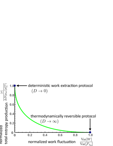
Figure 1: Normalized total entropy production versus normalized work fluctuation plotted along the stationary solution (25). Here, $\Delta D(p_{\mathrm{ini}}||p^{\mathrm{can}}_{\lambda_{0}}):=D(p_{\mathrm{ini}}||p^{\mathrm{can}}_{\lambda_{0}})-D_{0}(p_{\mathrm{ini}}||p^{\mathrm{can}}_{\lambda_{0}})$, with $D_{0}$ defined in Eq. (47) (see also Eq. (49)) and $\mathcal{F}_{\lambda_{0}}(x_{0})$ is the nonequilibrium free energy (44). The green curve gives the lower bound of the total entropy production for a given work fluctuation, thereby showing the boundary of the trade-off relation between work fluctuation and the total entropy production (see Sec. IV). The two blue dots at both ends of the curve show the values of $(\text{Var}[W],\left\langle\sigma\right\rangle)$ obtained from the deterministic work extraction protocol (49) and the thermodynamically reversible protocol (43).

By substituting the solution (26) into the normalization condition (18), we obtain

$$1=\sum_{\Gamma}\tilde{P}[\Gamma^{\dagger}]=\sum_{\Gamma}P[\Gamma|x_{0}]q(x_{0})=\sum_{x_{0}}q(x_{0}),$$ (28)

where we use Eq. (2), i.e., $\sum_{x_{1},x_{2},\cdots,x_{N}}P[\Gamma|x_{0}]=1$, in deriving the last equality in Eq. (28). From Eq. (28), either $C$ or $D$ is fixed and from the constraint $\text{Var}[W]=\Delta^{2}_{W}$, the other parameter is determined. By determining $C$ and $D$ in this way, Eq. (26) give the stationary solution to Eq. (20).

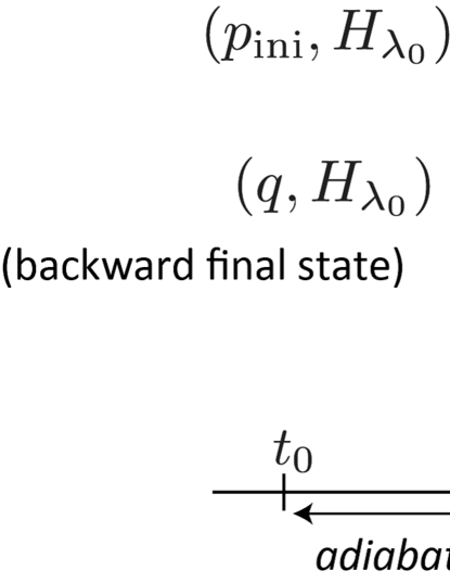
Figure 2: Protocol achieving the stationary solution (26). A change in the state of the system is shown vertically and a change in the Hamiltonian of the system is shown horizontally. The forward protocol consists of an adiabatic process followed by a quasi-static process. Here, by the quasi-static process, we mean that a change in the Hamiltonian of the system is slow compared with the relaxation of the system via the interaction with the heat bath. At the beginning of the quasi-static process, the state of the system changes from $p_{\mathrm{ini}}$ to a thermalized state $q$ given in Eq. (27). In $(q,H_{q})$, $H_{q}$ represents the Hamiltonian whose canonical distribution is $q$. The backward protocol consists of a quasi-static process followed by an adiabatic process. Because the total entropy production of the forward process is nonvanishing, the final state of the backward process $q$ differs from the initial state of the forward process.

III.3 Explicit protocol that satisfies the stationary condition (20)

Now let us consider a protocol $\{\lambda_{i}\}$ that gives the stationary solution (26). Before deriving the explicit protocol, we briefly explain the themodynamically reversible protocol for nonequilibrium initial and final states, i.e., the protocol achieving $\left\langle\sigma\right\rangle=0$. Let us denote the forward and backward probability distributions as $P^{\prime}[\Gamma]$ and $\tilde{P^{\prime}}[\Gamma^{\dagger}]$, respectively. The condition $P^{\prime}[\Gamma]=\tilde{P^{\prime}}[\Gamma^{\dagger}]$ for $\forall\Gamma$ is satisfied if and only if the protocol is given by the thermodynamically reversible protocol. As discussed in Refs. Esposito2 ; Parrondo , this protocol can be constructed from the combination of a quench of the Hamiltonian with a quasi-static process.

If we regard Eq. (26) as a condition on the backward protocol, i.e., $P^{\prime}[\Gamma]=\tilde{P}[\Gamma^{\dagger}]$ and $\tilde{P^{\prime}}[\Gamma^{\dagger}]=P[\Gamma|x_{0}]q(x_{0})$, we find that Eq. (26) is equivalent to the condition that the backward process is given by a thermodynamically reversible protocol that starts from $p^{\mathrm{can}}_{\lambda_{N}}(x_{N})$ and ends at $q(x_{0})$. If we denote $H_{q}$ as a Hamiltonian whose canonical distribution with the inverse temperature $\beta$ is equal to $q$, the thermodynamically reversible protocol of the backward process is given as follows (see also Fig. 2):

1. Quasi-statically change the Hamiltonian from $H_{\lambda_{N}}$ to $H_{q}$. Then, the state of the system changes from $p^{\mathrm{can}}_{\lambda_{N}}(x_{N})$ to $q(x_{0})$.

2. Adiabatically change the Hamiltonian from $H_{q}$ to $H_{\lambda_{0}}$. Note that the probability distribution of the system $q(x_{0})$ does not change during this process.

The adiabatic change of the Hamiltonian is possible if we consider either a classical system or a quantum system such that $H_{q}$ and $H_{\lambda_{0}}$ commute with each other. In this case, we can realize an adiabatic process by a sudden quench of the Hamiltonian. If $H_{q}$ and $H_{\lambda_{0}}$ do not commute with each other, we need to keep the system detached from the heat bath and change the Hamiltonian slowly so that the quantum adiabatic theorem holds.

The quasi-static process keeps the total entropy production vanishing. The adiabatic process neither changes the Shannon entropy of the system nor generates heat. The total entropy production during the above backward protocol vanishes and a thermodynamically reversible protocol for the backward process is obtained. We can also derive the forward protocol from the time-reversal of the backward protocol as follows (see also Fig. 2):

1. Adiabatically change the Hamiltonian from $H_{\lambda_{0}}$ to $H_{q}$.

2. Quasi-statically change the Hamiltonian from $H_{q}$ to $H_{\lambda_{N}}$. Note that we change the Hamiltonian sufficiently slow so that the state of the system equilibrates at every step. Thus, the state of the system first changes from $p_{\mathrm{ini}}(x_{0})$ to $q(x_{0})$ via thermalization and then isothermally changes to $p^{\mathrm{can}}_{\lambda_{N}}(x_{N})$.

Next, let us derive explicit forms of the forward and backward probability distributions. Because an adiabatic process does not change the distribution of the system, and a quasi-static process gives the final state which is equal to the canonical distribution no matter what the initial state of the system is, the forward probability distribution is given by

$$P[\Gamma]=p_{\mathrm{ini}}(x_{0})p^{\mathrm{can}}_{\lambda_{N}}(x_{N}),$$ (29)

and the backward probability distribution is given by

$$\tilde{P}[\Gamma^{\dagger}]=p^{\mathrm{can}}_{\lambda_{N}}(x_{N})q(x_{0}).$$ (30)

Here, we note that $H_{\lambda_{1}}=H_{q}$ and the quasi-static process of the backward process ends at $\tilde{t}=\tilde{t}_{N-1}(=t_{1})$ with the corresponding canonical distribution $q(x_{0})$. We also note that $E_{\lambda_{N}}(x_{N})$ is fixed. Therefore, $P[\Gamma]$ does not depend on any $\{E_{\lambda_{i}}(y_{i})\}$, and $\tilde{P}[\Gamma^{\dagger}]$ depends only on $E_{\lambda_{1}}(x_{0})=E_{q}(x_{0})$.

From the above argument, we find that

$$\frac{\delta S}{\delta\tilde{P}[\Gamma^{\dagger}]}=0\ \Rightarrow\ \frac{\delta P[\Gamma]}{\delta E_{\lambda_{i}}(y_{i})}=0\ \ \text{for }\ \forall E_{\lambda_{i}}(y_{i}).$$ (31)

By noting that $S$ is a functional of $\{E_{\lambda_{i}}(y_{i})\}$ through its dependences on $P[\Gamma]$ and $\tilde{P}[\Gamma^{\dagger}]$, Eq. (31) can be used to show that Eq. (19) is satisfied by the stationary solutions obtained from Eq. (20).

IV Proof of the trade-off relation between work fluctuation and the total entropy production

In this section, we show that the stationary solution (26) gives the global minimum of the work fluctuation for a given total entropy production. We use this stationary solution and denote the total entropy production $\left\langle\sigma\right\rangle$ as

$$\Sigma:=\sum_{x_{0}}p_{\mathrm{ini}}(x_{0})\ln\frac{p_{\mathrm{ini}}(x_{0})}{q(x_{0})},$$ (32)

and the work fluctuation $\text{Var}[\beta W]$ as

$$\beta^{2}\Delta^{2}_{W} := \sum_{x_{0}}p_{\mathrm{ini}}(x_{0})\left[\ln\frac{p^{\mathrm{can}}_{\lambda_{0}}(x_{0})}{q(x_{0})}\right]^{2}$$ (33)

$$-\left(\sum_{x_{0}}p_{\mathrm{ini}}(x_{0})\ln\frac{p^{\mathrm{can}}_{\lambda_{0}}(x_{0})}{q(x_{0})}\right)^{2}.$$

Note that Eqs. (32) and (33) are shown by the green solid curve in Fig. 1.

Now we consider an arbitrary protocol and denote its forward and backward probabilities as $P[\Gamma]$ and $\tilde{P}[\Gamma^{\dagger}]$, respectively. Let us divide the total entropy production of an arbitrary protocol into two parts:

$$\sigma[\Gamma]=\ln\frac{P[\Gamma]}{\tilde{P}[\Gamma^{\dagger}]}=\sigma_{q}(x_{0})+\Delta\sigma[\Gamma],$$ (34)

where

$$\sigma_{q}(x_{0})=\ln\frac{p_{\mathrm{ini}}(x_{0})}{q(x_{0})},\ \ \Delta\sigma[\Gamma]=\ln\frac{P_{q}[\Gamma]}{\tilde{P}[\Gamma^{\dagger}]}.$$ (35)

Note that $P_{q}[\Gamma]:=P[\Gamma|x_{0}]q(x_{0})$ is normalized to unity as can be seen from Eq. (28). We use Eq. (34) to calculate $\left\langle\sigma\right\rangle$ as

$$\left\langle\sigma\right\rangle=\Sigma+\left\langle\Delta\sigma\right\rangle.$$ (36)

In what follows, we derive the global minimum of the work fluctuation for a given total entropy production $\left\langle\sigma\right\rangle=\Sigma$. Then, we have $\left\langle\Delta\sigma\right\rangle=0$ from Eq. (36), and $\text{Var}[\beta W]$ takes the form

$$\text{Var}[\beta W] = \text{Var}\left[\ln\frac{p^{\mathrm{can}}_{\lambda_{0}}}{q}+\Delta\sigma\right]$$ (37)

$$= \beta^{2}\Delta^{2}_{W}+2\left\langle\Delta\sigma\ln\frac{p^{\mathrm{can}}_{\lambda_{0}}}{q}\right\rangle+\left\langle(\Delta\sigma)^{2}\right\rangle,$$

By using the relation $\mathrm{e}^{W_{0}(z)}=\frac{z}{W_{0}(z)}$, we have

$$2\left\langle\Delta\sigma\ln\frac{p^{\mathrm{can}}_{\lambda_{0}}}{q}\right\rangle=2D\sum_{\Gamma}P_{q}[\Gamma]\Delta\sigma[\Gamma]\geq 0,$$ (38)

where the last inequality results from $D\geq 0$ and the nonnegativity of the Kullback-Leibler divergence between $P_{q}[\Gamma]$ and $\tilde{P}[\Gamma^{\dagger}]$ Cover :

$$D(P_{q}||\tilde{P})=\sum_{\Gamma}P_{q}[\Gamma]\Delta\sigma[\Gamma]\geq 0.$$ (39)

Finally, we combine Eqs. (37) and (38) and use $\left\langle(\Delta\sigma)^{2}\right\rangle\geq 0$ to obtain

$$\text{Var}[W]-\Delta^{2}_{W}\geq 0.$$ (40)

We have shown that the stationary solution (27) gives the minimum of the work fluctuation for a given total entropy production, and the lower bound is shown by the green solid curve in Fig. 1.

We can also consider the minimum value of $\left\langle\sigma\right\rangle$ for a given (constant) work fluctuation $\text{Var}[W]=\Delta^{2}_{W}$ in a manner similar to the derivation of Eq. (40). The result is equivalent to Eq. (40); Eq. (27) gives the minimum value of $\left\langle\sigma\right\rangle$ for a given $\text{Var}[W]$.

The equality in (40) is satisfied if and only if $\Delta\sigma[\Gamma]=0$ for $\forall\Gamma$, which is equivalent to the stationary solution (26). Therefore, the lower bound of the total entropy production for a given work fluctuation, depicted by the green solid curve in Fig. 1, is achieved if and only if the protocol is the one shown in Fig. 2.

V Some special points of the trade-off relation

In this section, we consider some special points of the stationary solution, namely the limit of vanishing total entropy production ($D\rightarrow\infty$) and that of vanishing work fluctuation ($D\rightarrow 0$). Then, we compare those special points with the previously obtained results for the thermodynamically reversible protocol Parrondo ; Esposito2 ; Hasegawa ; Takara and the deterministic work extraction protocol Aberg ; Horodecki .

V.1 Thermodynamically reversible protocol

For $D=\infty$, we can use the asymptotic form of $W_{0}$ for large values of $z$: $W_{0}(z)=\ln(z)-\ln\ln(z)+\cdots$. Let us consider the normalization condition of $q(x_{0})$ by expanding $W_{0}$ up to the most divergent term:

$$1=\sum_{x_{0}}q(x_{0})=\frac{C}{D}+O\left(\frac{\ln D}{D}\right).$$ (41)

Then, using Eq. (27), we obtain

$$q(x_{0})=p_{\mathrm{ini}}(x_{0})\hskip 5.69054pt\text{ for }D=\infty.$$ (42)

From Eqs. (32) and (33), we find that the total entropy production vanishes; however, the amount of work fluctuation remains nonvanishing:

$$\left\langle\sigma\right\rangle=0,\ \text{Var}[W]=\text{Var}[\mathcal{F}_{\lambda_{0}}],$$ (43)

where

$$\mathcal{F}_{\lambda_{0}}(x_{0}):=F_{\lambda_{0}}+kT\ln\frac{p_{\mathrm{ini}}(x_{0})}{p^{\mathrm{can}}_{\lambda_{0}}(x_{0})}$$ (44)

is the initial nonequilibrium free energy Esposito2 ; Deffner , which quantifies the maximum value of the average extractable work if the system is initially prepared in a nonequilibrium state. Note that the maximum value is achieved in this case:

$$\left\langle W\right\rangle=\left\langle\mathcal{F}_{\lambda_{0}}\right\rangle-F_{\lambda_{N}},$$ (45)

and the protocol (i) and (ii) given in Sec. III.3 reproduces the thermodynamically reversible protocol discussed in Ref Esposito .

V.2 Deterministic work extraction protocol

If $D=0$, the Taylor expansion of $W_{0}$ around $0$ gives $W_{0}(z)=z-z^{2}+\cdots$. From Eq. (27), we obtain

$$q(x_{0})=p^{\mathrm{can}}_{\lambda_{0}}(x_{0})\mathrm{e}^{C}+O(D).$$ (46)

We note that the support of $q(x_{0})$ is the same as that of $p_{\mathrm{ini}}(x_{0})$. By defining $X$ as a set of labels corresponding to the nonvanishing initial probabilities, i.e., $X=\{x|p_{\mathrm{ini}}(x_{0})>0\}$, the normalization condition (28) determines $C=D_{0}(p_{\mathrm{ini}}||p^{\mathrm{can}}_{\lambda_{0}})$, where

$$D_{0}(p_{\mathrm{ini}}||p^{\mathrm{can}}_{\lambda_{0}})=-\ln\sum_{x_{0}\in X}p^{\mathrm{can}}_{\lambda_{0}}(x_{0})$$ (47)

is the Renyi-zero divergence Renyi . We then obtain

$$q(x_{0}):=\biggl{\{}\begin{array}[]{lc}p^{\mathrm{can}}_{\lambda_{0}}(x_{0})\mathrm{e}^{D_{0}(p_{\mathrm{ini}}||p^{\mathrm{can}}_{\lambda_{0}})}&\text{for }x_{0}\in X;\\ 0&\text{for }x_{0}\not\in X,\end{array}$$ (48)

for $D=0$. Substituting Eq. (48) into Eqs. (32) and (33), we have

$$\left\langle\sigma\right\rangle=D(p_{\mathrm{ini}}||p^{\mathrm{can}}_{\lambda_{0}})-D_{0}(p_{\mathrm{ini}}||p^{\mathrm{can}}_{\lambda_{0}}),\ \text{Var}[W]=0.$$ (49)

Since the work fluctuation vanishes, the extractable work does not fluctuate and is given by

$$W[\Gamma]=kTD_{0}(p_{\mathrm{ini}}||p^{\mathrm{can}}_{\lambda_{0}})+F_{\lambda_{0}}-F_{\lambda_{N}}.$$ (50)

Let us define a Hamiltonian $H^{*}_{\lambda_{0}}$ which gives the canonical distribution (48) as follows:

$$H^{*}_{\lambda_{0}} := \sum_{x_{0}\in X}E_{\lambda_{0}}(x_{0})\left|E_{\lambda_{0}}(x_{0})\right\rangle\left\langle E_{\lambda_{0}}(x_{0})\right|$$ (51)

$$+ \sum_{x_{0}\not\in X}V\left|E_{\lambda_{0}}(x_{0})\right\rangle\left\langle E_{\lambda_{0}}(x_{0})\right|,\ V\rightarrow\infty.$$

Then, $H_{q}=H^{*}_{\lambda_{0}}$ and the protocol achieving Eq. (48) is given as follows: (i) Adiabatically change the Hamiltonian from $H_{\lambda_{0}}$ to $H^{*}_{\lambda_{0}}$. (ii) Quasi-statically change the Hamiltonian from $H^{*}_{\lambda_{0}}$ to $H_{\lambda_{N}}$. Note that at the beginning of (ii), the state of the system is thermalized and is given by Eq. (48). Note that the $kTD_{0}(p_{\mathrm{ini}}||p^{\mathrm{can}}_{\lambda_{0}})$ term in the extractable work (50) is equal to the increased equilibrium free energy of the system via the adiabatic change of the Hamiltonian:

$$kTD_{0}(p_{\mathrm{ini}}||p^{\mathrm{can}}_{\lambda_{0}})=F^{*}_{\lambda_{0}}-F_{\lambda_{0}},$$ (52)

where $F^{*}_{\lambda_{0}}:=-\beta^{-1}\ln\text{Tr}\exp(-\beta H^{*}_{\lambda_{0}})$. The protocol (i) and (ii) reproduces the deterministic work extraction protocol discussed in Ref. Aberg by changing the energy levels of the system and by attaching a heat bath to the system. In Appendix A.3, we consider the setups used in the single-shot statistical mechanics and reproduce the deterministic work extraction protocol discussed in Ref. Horodecki .

VI Conclusion

We have studied the minimum of the total entropy production for a given work fluctuation. By applying the variational method, we have obtained the stationary solution (26). From the analysis performed in Sec. IV, the solution (26) is found to give the minimum of the total entropy production for a given work fluctuation in the region expressed by the green curve in Fig. 1. The protocol which achieves the minimum is shown to be constructed from an adiabatic process and a quasi-static process, as shown in Fig. 2. The obtained protocol describes an efficient way of transforming a nonequilibrium initial state to a thermalized state, thereby suppressing both work fluctuation and total entropy production. In particular, we have discussed two special ways of approaching equilibrium; one discussed in Sec. V.2 allows the system to achieve the limit of vanishing work fluctuation, and the other discussed in Sec. V.1 adiabatically transforms the system to achieve the limit of vanishing total entropy production. Below, we summarize and discuss some outstanding issues and outlooks.

We have considered the variational problem (19) with respect to the protocol $\{\lambda_{i}\}$. In Sec. III.2, we have shown that Eq. (19) is satisfied by the stationary solution to the variation of the Lagrange function with the backward probability distribution. However, we have found that if we consider a variation with respect to the forward probability distribution, the stationary solution does not satisfy Eq. (19). The origin of this asymmetry between the forward and backward probability distributions in the variational problem deserves further clarification.

In Sec. III.3, we have used the detailed fluctuation theorem and the thermodynamic reversibility of the backward protocol and obtained an explicit protocol that satisfies the stationary solutions. This method of obtaining the protocol of the system can be applied to other problems. For instance, if we place constraints on the extractable work and the total entropy production as $\alpha\sigma[\Gamma]-(1-\alpha)\beta W[\Gamma]=\text{const.}$, we obtain the protocol discussed in Ref. Funo , which minimizes the sum of the standard deviation of work and that of the total entropy production.

We have not considered an optimization of the protocol in a finite time, which has gathered considerable interest in recent years Schmiedl ; Aurell ; Adolfo . It is challenging to extend the obtained work-fluctuation dissipation trade-off relation to such finite-time optimization.

We have considered the settings used in the single-shot statistical mechanics and derived the detailed fluctuation theorem in Appendix A. This analysis together with the reproduced deterministic work extraction protocol from the obtained trade-off relation helps us gain deeper understanding of the relations between different approaches to thermodynamics in small systems such as the fluctuation theorems and the single-shot statistical mechanics. We note that in Ref. Richens , the authors investigated a connection between the deterministic work extraction protocol and the second law of thermodynamics by examining the amount of average work subject to constraints on the difference between the stochastic work and the average work.

Appendix A Thermal operations and the detailed fluctuation theorem

Usual setups in the single-shot statistical mechanics Horodecki are different from the setups used in stochastic thermodynamics and fluctuation theorems Seifert . Here we discuss how the above two setups are related so that we can compare the vanishing work fluctuation limit of the obtained trade-off relation based on the detailed fluctuation theorem with the single-shot statistical mechanics. We first derive the detailed fluctuation theorem using a setting similar to that used in Ref. Horodecki , that is, the thermal operation. Then we reproduce the deterministic work extraction protocol on the basis of the obtained trade-off relation.

A.1 Thermal operations

In this section, we review the thermal operation which is used in Ref. Horodecki to derive the deterministic work extraction protocol. From the experimental point of view, the thermal operation models a state transformation of a system interacting with a single heat bath under the assumption that an arbitrary control on the system-bath coupling is possible.

Let us assume that the initial state of the system does not have coherence in the energy eigenbasis. We follow Ref. Horodecki and treat the external driving of the Hamiltonian as an effective dynamics of a fixed Hamiltonian of a larger system $CSW$ explained as follows. Here, the $i$-th step of the protocol changes the Hamiltonian of the system as $H_{\lambda_{i}}\rightarrow H_{\lambda_{i+1}}$ (modeled by the larger system $CSW$) followed by the relaxation of the system in contact with the heat bath $B$. We introduce a qubit system $C$ which switches the Hamiltonian of the system $S$ between $H_{\lambda_{i}}$ and $H_{\lambda_{i+1}}$ depending on the state of the qubit $\left|0\right\rangle_{C}$ or $\left|1\right\rangle_{C}$. We also introduce the work storage system $W$ which stores the work extracted from the system and define its Hamiltonian as $H_{W}:=\sum_{w}w\left|w\right\rangle\left\langle w\right|_{W}$. Note that if we only focus on the deterministic work extraction protocol, it is enough to take a qubit system as the work storage Horodecki . In the present setup, we allow fluctuations in the extracted work. Then the total Hamiltonian of the composite system $CSW$ reads

$$H^{\mathrm{tot}}:=\left|0\right\rangle\left\langle 0\right|_{C}\otimes H_{\lambda_{i}}+\left|1\right\rangle\left\langle 1\right|_{C}\otimes H_{\lambda_{i+1}}+H_{W}.$$ (53)

We model a general state transformation of the system due to the interaction with the heat bath by applying an arbitrary total-energy conserving unitary operator on the total system including the heat bath $B$, and take the partial trace over $B$:

$$\mathcal{E}_{\text{thermal}}(\rho):=\text{Tr}_{B}\left[U\left(\rho\otimes\rho^{B}_{\mathrm{can}}\right)U^{\dagger}\right].$$ (54)

Here $\rho^{B}_{\mathrm{can}}=\exp(-\beta H^{B})/Z_{B}$ and $H^{B}$ are the canonical distribution and the Hamiltonian of the heat bath, respectively, and $U$ is an arbitrary unitary operator that satisfies

$$[U,H^{\mathrm{tot}}+H^{B}]=0.$$ (55)

However, $U$ is not limited to the form of $\exp(-\mathrm{i}(H^{\mathrm{tot}}+H^{B})t)$ which describes the time evolution of an isolated quantum system. Implementing the thermal operation (54) in an experiment is challenging because it generally requires a detailed control of the interaction between the system and the heat bath. However, from a theoretical point of view, Eq. (54) can be used to search for a boundary on the allowed state transformation of the system set by thermodynamics in an extreme situation such that we have an unlimited control over the system-bath interaction. To study this boundary, thermo-majorization is introduced in Ref. Horodecki which establishes a quasiorder $\succ_{\mathrm{th}}$ on the density matrix of the system, giving an “ordering” with respect to the canonical distribution of the system. To define this quasiorder $\rho\succ_{\mathrm{th}}\sigma$, let us denote the diagonal element of $\rho$ and that of $\sigma$ as $\rho(x)$ and $\sigma(x)$, respectively. We rearrange the label $x$ according to the following order:

$$\frac{\rho(1)}{\mathrm{e}^{-\beta E(1)}/Z}\geq\frac{\rho(2)}{\mathrm{e}^{-\beta E(2)}/Z}\geq\frac{\rho(3)}{\mathrm{e}^{-\beta E(3)}/Z}\geq\cdots.$$ (56)

Then, we plot the Lorenz curve denoted as $(\frac{\mathrm{e}^{-\beta H}}{Z},\rho)$ in the $(X,Y)$ plane as in Fig. 3 in which each point is given by

$$\biggl{\{}\left(\frac{\mathrm{e}^{-\beta E(1)}}{Z},\ \rho(1)\right),\left(\sum_{i=1}^{2}\frac{\mathrm{e}^{-\beta E(i)}}{Z},\sum_{i=1}^{2}\rho(i)\right),$$

$$\ \ \left(\sum_{i=1}^{3}\frac{\mathrm{e}^{-\beta E(i)}}{Z},\sum_{i=1}^{3}\rho(i)\right),\ \cdots,\ (1,1)\biggr{\}}.$$ (57)

Note that the ordering (56) ensures that the curve (57) is convex. If the Lorenz curve $(\frac{\mathrm{e}^{-\beta H}}{Z},\sigma)$ is below $(\frac{\mathrm{e}^{-\beta H}}{Z},\rho)$, we say $\rho$ thermo-majorizes $\sigma$ and write as $\rho\succ_{\mathrm{th}}\sigma$ Majorization2 . An important property is of thermo-majorization is that $\rho\succ_{\mathrm{th}}\rho^{\mathrm{can}}$ holds for any $\rho$ and $\rho^{\mathrm{can}}:=\exp(-\beta H^{\mathrm{tot}})/Z$. Therefore, all states thermo-majorize the canonical distribution. It has been shown in Ref. Horodecki that if $[\rho,H^{\mathrm{tot}}]=[\sigma,H^{\mathrm{tot}}]=0$, $\rho$ can be transformed into $\sigma$ via a thermal operation if and only if $\rho\succ_{\mathrm{th}}\sigma$. Note that the canonical distribution is a fixed point of the thermal operation, i.e., $\mathcal{E}_{\text{thermal}}(\rho^{\mathrm{can}})=\rho^{\mathrm{can}}$.

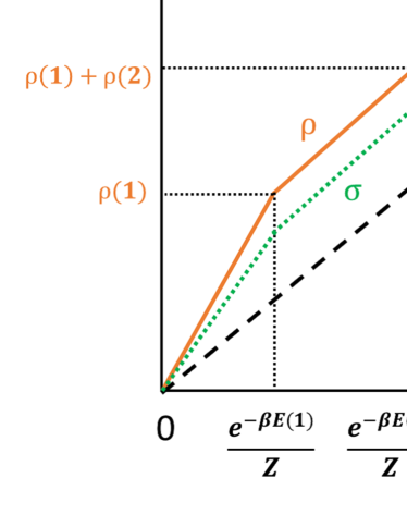
Figure 3: Lorenz curve and the thermo-majorization criterion. The Lorenz curve shows a nonuniformity of the state of the system with respect to the canonical distribution, and gives a graphical representation of the quasiordering $\succ_{\mathrm{th}}$, i.e., the thermomajorization. We plot $\{\sum_{i=1}^{k}\frac{\mathrm{e}^{-\beta E(i)}}{Z}\}$ and $\{\sum_{i=1}^{k}p(i)\}$ in the $(X,Y)$ plane, where the curve $p=\rho$ is shown by the orange curve, $p=\sigma$ by the green dotted curve and $p=\rho_{\mathrm{can}}=\frac{\mathrm{e}^{-\beta H}}{Z}$ by the black dashed line. The thermo-majorization criterion tells us that the state $\rho$ can be transformed into $\sigma$ via a thermal operation if the Lorenz curve $(\sigma,\frac{\mathrm{e}^{-\beta H}}{Z})$ is below that ot $(\rho,\frac{\mathrm{e}^{-\beta H}}{Z})$. Here, the Lorenz curves are plotted for $\rho$ and $\sigma$ having the same rearranged orderings as in Eq. (56).

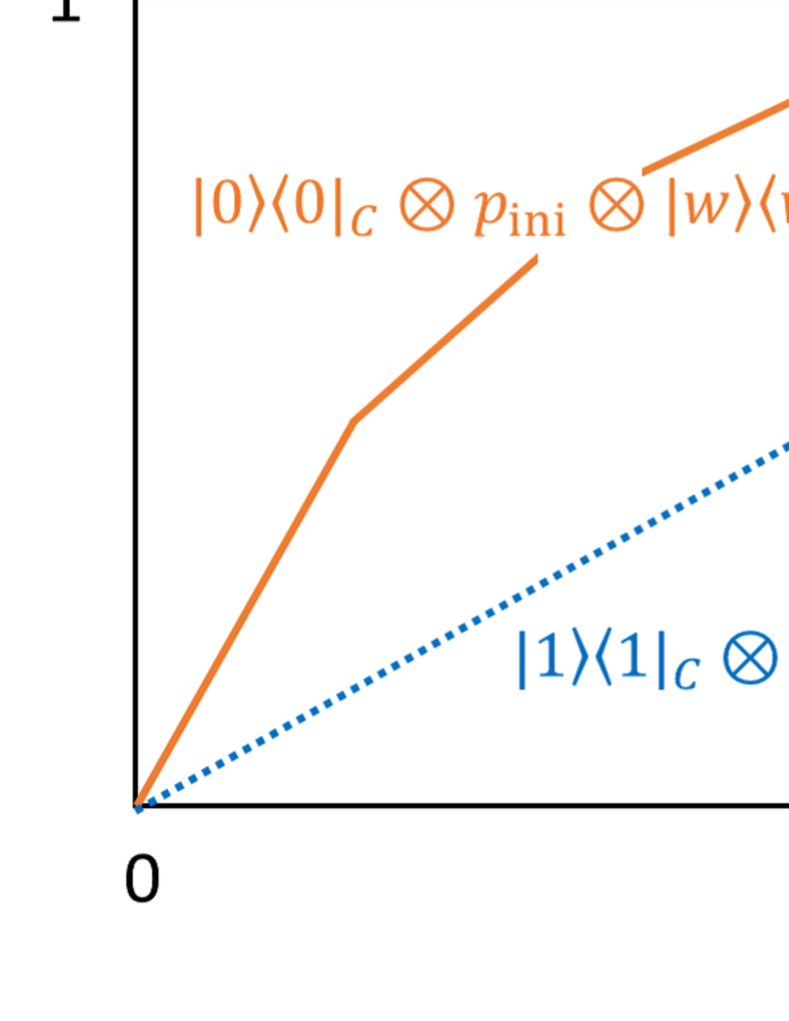
Figure 4: (a) Lorenz curves corresponding to the process shown in Eq. (73). If $w-u\leq 0$, the blue line is below the orange curve and the transition (73) is possible. (b) Lorenz curves corresponding to the process shown in Eq. (75). If $v-w\leq kT\ln\frac{Z_{\lambda_{N}}}{Z^{*}_{\lambda_{0}}}$, the blue curve is below the orange curve and therefore the transition (75) is possible.

A.2 Derivation of the detailed fluctuation theorem

We use the Hamiltonian (53) and consider a transition probability from

$$\left|0,x_{i},u\right\rangle:=\left|0\right\rangle_{C}\otimes\left|E_{\lambda_{i}}(x_{i})\right\rangle\otimes\left|u\right\rangle_{W}$$ (58)

to

$$\left|1,x_{i+1},w\right\rangle:=\left|1\right\rangle_{C}\otimes\left|E_{\lambda_{i+1}}(x_{i+1})\right\rangle\otimes\left|w\right\rangle_{W}.$$ (59)

Note that the Hamiltonian of the system changes from $H_{\lambda_{i}}$ to $H_{\lambda_{i+1}}$ during this process. The transition probability can be calculated by using Eq. (54) as

$$p[(x_{i},u)\rightarrow(x_{i+1},w)]$$

$$:=\sum_{a,b}\frac{\mathrm{e}^{-\beta E^{B}_{a}}}{Z^{B}}\bigl{|}\left\langle 1,x_{i+1},w\right|\left\langle\varphi^{B}_{b}\right|U\left|\varphi^{B}_{a}\right\rangle\left|0,x_{i},u\right\rangle\bigr{|}^{2}.$$ (60)

Here, $\{\left|\varphi^{B}_{a}\right\rangle\}$ is the set of energy eigenvectors of the heat bath. Let us also define the backward transition probability by using the Hermitian conjugate operator of $U$:

$$\tilde{p}[(x_{i+1},w)\rightarrow(x_{i},u)]$$

$$:=\sum_{a,b}\frac{\mathrm{e}^{-\beta E^{B}_{b}}}{Z^{B}}\bigl{|}\left\langle 0,x_{i},u\right|\left\langle\varphi^{B}_{a}\right|U^{\dagger}\left|\varphi^{B}_{b}\right\rangle\left|1,x_{i+1},w\right\rangle\bigr{|}^{2}.$$ (61)

Since thermal operations preserve the total energy [see Eq. (55)], we obtain

$$E_{\lambda_{i}}(x_{i})+u+E^{B}_{a}=E_{\lambda_{i+1}}(x_{i+1})+w+E^{B}_{b}$$ (62)

for the transition $\left|\varphi^{B}_{a}\right\rangle\left|0,x_{i},u\right\rangle\rightarrow\left|1,x_{i+1},w\right\rangle\left|\varphi^{B}_{b}\right\rangle$. By substituting Eq. (62) into Eq. (60) and using the relation

$$\bigl{|}\left\langle 1,x_{i+1},w\right|\left\langle\varphi^{B}_{b}\right|U\left|\varphi^{B}_{a}\right\rangle\left|0,x_{i},u\right\rangle\bigr{|}^{2}$$

$$=\bigl{|}\left\langle 0,x_{i},u\right|\left\langle\varphi^{B}_{a}\right|U^{\dagger}\left|\varphi^{B}_{b}\right\rangle\left|1,x_{i+1},w\right\rangle\bigr{|}^{2},$$ (63)

we obtain a relation between the forward and backward transition probabilities:

$$p[(x_{i},u)\rightarrow(x_{i+1},w)]$$

$$= \sum_{a,b}\biggl{[}\frac{1}{Z^{B}}\mathrm{e}^{-\beta(E^{B}_{b}+E_{\lambda_{i+1}}(x_{i+1})-E_{\lambda_{i}}(x_{i})+w-u)}$$

$$\times\bigl{|}\left\langle 1,x_{i+1},w\right|\left\langle\varphi^{B}_{b}\right|U\left|\varphi^{B}_{a}\right\rangle\left|0,x_{i},u\right\rangle\bigr{|}^{2}\biggr{]}$$

$$= \mathrm{e}^{-\beta(E_{\lambda_{i+1}}(x_{i+1})-E_{\lambda_{i}}(x_{i})+w-u)}\tilde{p}[(x_{i+1},w)\rightarrow(x_{i},u)].$$

Now the heat absorbed by the system is defined as the energy decrease of the heat bath:

$$Q[(x_{i},u)\rightarrow(x_{i+1},w)]=-(E^{B}_{b}-E^{B}_{a}).$$ (64)

It follows from Eq. (62) that this definition of heat is equal to the energy increase of the composite system $CSW$:

$$Q[(x_{i},u)\rightarrow(x_{i+1},w)]:=E_{\lambda_{i+1}}(x_{i+1})-E_{\lambda_{i}}(x_{i})+w-u.$$ (65)

Using the definition of the heat absorbed by the system, we find that the detailed balance condition is satisfied:

$$\frac{p[(x_{i},u)\rightarrow(x_{i+1},w)]}{\tilde{p}[(x_{i+1},w)\rightarrow(x_{i},u)]}=\mathrm{e}^{-\beta Q[(x_{i},u)\rightarrow(x_{i+1},w)]}.$$ (66)

Now, we can define the forward probability distribution as (from now on, we rewrite $u\rightarrow u_{i}$ and $w\rightarrow w_{i+1}$ for convenience)

$$P[\Gamma]:=p_{\mathrm{ini}}(x_{0})\prod_{i=0}^{N-1}p[(x_{i},u_{i})\rightarrow(x_{i+1},w_{i+1})],$$ (67)

and the backward probability distribution as:

$$\tilde{P}[\Gamma^{\dagger}]:=p^{\mathrm{can}}_{\lambda_{N}}(x_{N})\prod_{i=0}^{N-1}\tilde{p}[(x_{N-i},w_{N-i})\rightarrow(x_{N-i-1},u_{N-i-1})].$$ (68)

We also define the total heat absorbed by the system as

$$Q[\Gamma]:=\sum_{i=0}^{N-1}Q[(x_{i},u_{i})\rightarrow(x_{i+1},w_{i+1})].$$ (69)

We then arrive at the detailed fluctuation theorem:

$$\frac{P[\Gamma]}{\tilde{P}[\Gamma^{\dagger}]}=\mathrm{e}^{\sigma[\Gamma]},$$ (70)

where the total entropy production is defined by Eq. (7). We also note that the extractable work is equal to the total excited energy of the work storage system:

$$W[\Gamma]=\sum_{i=0}^{N-1}(w_{i+1}-u_{i}).$$ (71)

A.3 Derivation of the deterministic work extraction protocol in Ref. Horodecki based on the trade-off relation

Let us consider thermal operations and derive a protocol which realizes Eq. (48). The first step is to define the total Hamiltonian as

$$H^{\mathrm{tot}}_{0}=H_{\lambda_{0}}\otimes\left|0\right\rangle\left\langle 0\right|_{C}+H^{*}_{\lambda_{0}}\otimes\left|1\right\rangle\left\langle 1\right|_{C}+H_{W},$$ (72)

where $H^{*}_{\lambda_{0}}$ is defined in Eq. (51). Then, we consider thermal operation that gives the following transition:

$$\left|0\right\rangle\left\langle 0\right|_{C}\otimes p_{\mathrm{ini}}\otimes\left|u\right\rangle\left\langle u\right|_{W}\longrightarrow\left|1\right\rangle\left\langle 1\right|_{C}\otimes p_{\mathrm{ini}}\otimes\left|w\right\rangle\left\langle w\right|_{W}.$$ (73)

Here, Eq. (73) describes an adiabatic process that changes the Hamiltonian from $H_{\lambda_{0}}$ to $H^{*}_{\lambda_{0}}$. From the thermo-majorization curve, the transition (73) is possible (i.e., there exists a unitary operator $U$) if $w-u=0$ from the Lorenz curve shown in Fig. 4 (a). The next step is to combine the $N-1$ steps into one and define the total Hamiltonian as

$$H^{\mathrm{tot}}_{1\rightarrow N}=H^{*}_{\lambda_{0}}\otimes\left|0\right\rangle\left\langle 0\right|_{C}+H_{\lambda_{N}}\otimes\left|1\right\rangle\left\langle 1\right|_{C}+H_{W},$$ (74)

and consider thermal operation that gives the following transition:

$$\left|0\right\rangle\left\langle 0\right|_{C}\otimes p_{\mathrm{ini}}\otimes\left|w\right\rangle\left\langle w\right|_{W}\longrightarrow\left|1\right\rangle\left\langle 1\right|_{C}\otimes p^{\mathrm{can}}_{\lambda_{N}}\otimes\left|v\right\rangle\left\langle v\right|_{W}.$$ (75)

Here, Eq. (75) describes a quasi-static process that changes the Hamiltonian from $H^{*}_{\lambda_{0}}$ to $H_{\lambda_{N}}$. From the Lorenz curve shown in Fig. 4 (b), the transition (75) is possible if $v-w$ is given by:

$$v-w=kT\ln\frac{Z_{\lambda_{N}}}{Z^{*}_{\lambda_{0}}}=F^{*}_{\lambda_{0}}-F_{\lambda_{N}},$$ (76)

where $Z^{*}_{\lambda_{0}}=\text{Tr}\exp(-\beta H^{*}_{\lambda_{0}})$ is the partition function. The extractable work in this case defined as the total excited energy of the work storage system and is given by

$$W[\Gamma]=v-u=kTD_{0}(p_{\mathrm{ini}}||p^{\mathrm{can}}_{\lambda_{0}})+F_{\lambda_{0}}-F_{\lambda_{N}},$$ (77)

which does not fluctuate. If we combine the two thermal operations (73) and (75) into one and take $H_{\lambda_{N}}=H_{\lambda_{0}}$, we reproduce the deterministic work extraction protocol and the extractable work $kTD_{0}(p_{\mathrm{ini}}||p^{\mathrm{can}}_{\lambda_{0}})$ from a nonequilibrium system as discussed in Ref. Horodecki . We note that from Eq. (77), we only need to prepare a qubit system for the work storage $W$, whose energy difference between the excited and ground states is given by $kTD_{0}(p_{\mathrm{ini}}||p^{\mathrm{can}}_{\lambda_{0}})+F_{\lambda_{0}}-F_{\lambda_{N}}$.

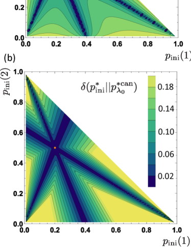
Figure 5: (a) Difference between Eq. (27) and Eq. (80) in the normalized total entropy production for different choices of the initial probability. The orange dot represents a point that satisfies $p_{\mathrm{ini}}=p^{\mathrm{can}}_{\lambda_{0}}$. We find that there is a wide region in which $p_{\mathrm{ini}}$ and $p^{\mathrm{can}}_{\lambda_{0}}$ are very different but the difference in the total entropy production is small. (b) Plot of $\delta(p^{*}_{\mathrm{ini}}||p^{*\mathrm{can}}_{\lambda_{0}})$ for different choices of the initial probability. Here, we plot for a three-level system and fix $p^{\mathrm{can}}_{\lambda_{0}}=\{0.2,0.5,0.3\}$.

Appendix B Comparison with related works

Here, we compare the main results presented in this paper with those in Ref. Funo . In Ref. Funo , two of the present authors derived the trade-off relation between work fluctuation and dissipation by implicitly assuming that the relation $\left\langle f\right\rangle_{\alpha}=\sum_{\Gamma}P[\Gamma]\frac{p_{\alpha}(x_{0})}{p_{\mathrm{ini}}(x_{0})}f(x_{0})$ holds even if we replace $\left\langle f\right\rangle_{\alpha}$ by the conventional expectation values $\left\langle f(x_{0})\right\rangle=\sum_{\Gamma}P[\Gamma]f(x_{0})$. Here, $p_{\alpha}(x)$ is defined by

$$p_{\alpha}(x_{0}):=[p_{\mathrm{ini}}(x_{0})]^{\alpha}[p^{\mathrm{can}}_{\lambda_{0}}(x_{0})]^{1-\alpha}\mathrm{e}^{(1-\alpha)D_{\alpha}(p_{\mathrm{ini}}||p^{\mathrm{can}}_{\lambda_{0}})}$$ (78)

with

$$D_{\alpha}(p_{\mathrm{ini}}||p^{\mathrm{can}}_{\lambda_{0}}):=\frac{1}{\alpha-1}\ln\left(\sum_{x}[p_{\mathrm{ini}}(x)]^{\alpha}[p^{\mathrm{can}}_{\lambda_{0}}(x)]^{1-\alpha}\right)$$ (79)

being the Renyi divergence Renyi . Those two expectation values agree only when the distance between $p_{\mathrm{ini}}(x_{0})$ and $p^{\mathrm{can}}_{\lambda_{0}}(x_{0})$ is small, and thus the lower bound of the work fluctuation-dissipation trade-off relation, i.e.,

$$\left\langle\sigma_{\alpha}\right\rangle = D(p_{\mathrm{ini}}||p_{\alpha}),$$ (80)

$$\text{Var}[W_{\alpha}] = \alpha^{2}\text{Var}[\mathcal{F}_{\lambda_{0}}],$$ (81)

derived in Ref. Funo does not, in general, hold for arbitrary nonequilibrium situations. However, we find that for wide choices of the initial probability distributions, the lower bound of the total entropy production for a given work fluctuation discussed in Ref. Funo gives numerical values close to those given by Eq. (32) as shown in Fig. 5 (a). Here, we plot the difference in the total entropy production

$$\Delta\sigma=\left\langle\sigma_{\alpha}\right\rangle-\left\langle\sigma_{q}\right\rangle$$ (82)

for a constant work fluctuation by changing the initial probability distribution $p_{\mathrm{ini}}(x_{0})$ in Fig. 5, (a).

We find from Fig. 5 (b) and Fig. 6 that if the $M-1$ components of the $M$-level initial probability distribution can be approximated by the canonical distribution, we have small $\Delta\sigma$. Here, in Fig. 6, we plot $\Delta\sigma$ against the quantity measuring the distance between the $M-1$ components of the initial probability distribution and those of the canonical distribution:

$$\delta(p^{*}_{\mathrm{ini}}||p^{*\mathrm{can}}_{\lambda_{0}}) := \min_{i}\delta(p^{(i)}_{\mathrm{ini}}||p^{(i),\mathrm{can}}_{\lambda_{0}})$$ (83)

$$= \min_{i}\frac{1}{2}\left|\sum_{x_{0}}p^{(i)}_{\mathrm{ini}}(x_{0})-p^{(i),\mathrm{can}}_{\lambda_{0}}(x_{0})\right|,$$

where the ($M-1$)-level probability distributions are defined as

$$p^{(i)}_{\mathrm{ini}}(x_{0}) = \biggl{\{}\frac{p_{\mathrm{ini}}(1)}{1-p_{\mathrm{ini}}(i)},\cdots,\frac{p_{\mathrm{ini}}(i-1)}{1-p_{\mathrm{ini}}(i)},\frac{p_{\mathrm{ini}}(i+1)}{1-p_{\mathrm{ini}}(i)},$$

$$\cdots,\frac{p_{\mathrm{ini}}(M)}{1-p_{\mathrm{ini}}(i)}\biggr{\}}.$$

$$p^{(i),\mathrm{can}}_{\lambda_{0}}(x_{0}) = \biggl{\{}\frac{p^{\mathrm{can}}_{\lambda_{0}}(1)}{1-p^{\mathrm{can}}_{\lambda_{0}}(i)},\cdots,\frac{p^{\mathrm{can}}_{\lambda_{0}}(i-1)}{1-p^{\mathrm{can}}_{\lambda_{0}}(i)},\frac{p^{\mathrm{can}}_{\lambda_{0}}(i+1)}{1-p^{\mathrm{can}}_{\lambda_{0}}(i)},$$

$$\cdots,\frac{p^{\mathrm{can}}_{\lambda_{0}}M)}{1-p^{\mathrm{can}}_{\lambda_{0}}(i)}\biggr{\}}.$$

Note that a protocol which gives Eqs. (80) and (81) is obtained by

$$P[\Gamma|x_{0}]p_{\alpha}(x_{0})=\tilde{P}[\Gamma^{\dagger}].$$ (84)

If we define the following Hamiltonian

$$H_{\alpha}=(1-\alpha)H^{*}_{\lambda_{0}}+\alpha H_{p_{\mathrm{ini}}},$$ (85)

we find that $p_{\alpha}$ is equal to the canonical distribution with respect to $H_{\alpha}$. By comparing Eq. (26) with Eq. (84), we find that the protocol achieving Eqs. (80) and (81) is given by the protocol discussed in Sec. III.3 with $H_{q}$ replaced by $H_{\alpha}$. We note that $H_{\alpha}$ can be obtained by a linear combination of $H^{*}_{\lambda_{0}}$ and $H_{p_{\mathrm{ini}}}$. On the other hand, $H_{q}$ cannot be written in a simple form unlike Eq. (85). If we consider the initial probability and the initial Hamiltonian such that $\Delta\sigma$ is sufficiently small, the protocol in Eq. (84) is easier to implement compared with that of Eq. (26).

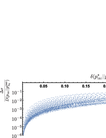
Figure 6: Normalized difference in the total entropy production $\frac{\Delta\sigma}{D(p_{\mathrm{ini}}||p^{\mathrm{can}}_{\lambda_{0}})}$ versus $\delta(p^{*}_{\mathrm{ini}}||p^{*\mathrm{can}}_{\lambda_{0}})$. The data is obtained for a three-level system and $p^{\mathrm{can}}_{\lambda_{0}}=\{0.2,0.5,0.3\}$. Each dot is obtained for different choices of $p_{\mathrm{ini}}$. If the distance $\delta(p^{*}_{\mathrm{ini}}||p^{*\mathrm{can}}_{\lambda_{0}})$ is small, two lower bounds of the total entropy production in Eqs. (32) and (80) give approximately equal numerical values. Each dot is obtained by randomly generating $p_{\mathrm{ini}}$.

References

- (1) J. M. R. Parrondo, J. M. Horowitz and T. Sagawa, Thermodynamics of information, Nat. Phys. 11, 131 (2015).
- (2) S. Deffner and E. Lutz, Information free energy for nonequilibrium states, arXiv:1201.3888.
- (3) M. Esposito and C. Van den Broeck, Second law and Landauer principle far from equilibrium, Euro. Phys. Lett. 95, 40004 (2011).
- (4) H.-H. Hasegawa, J. Ishikawa, K. Takara and D. J. Driebe, Generalization of the second law for a nonequilibrium initial state, Phys. Lett. A 374, 1001-1004 (2010).
- (5) K. Takara, H.-H. Hasegawa and K. J. Driebe, Generalization of the second law for a transition between nonequilibrium states, Phys. Lett. A 375, 88-92 (2010).
- (6) H. S. Leff and A. F. Rex, Maxwell’s Demon 2: Entropy, Classical and Quantum Information, Computing (Institute of Physics Publishing, 2003).
- (7) K. Maruyama, F. Nori and V. Vedral, Colloquium: The physics of Maxwell’s demon and information, Rev. Mod. Phys. 81, 1-23 (2009).
- (8) Thermodynamics of Information Processing in Small Systems, T. Sagawa (Springer, 2013).
- (9) J. C. Maxwell, Theory of Heat (Appleton, London, 1871).
- (10) L. Szilard, Z. Phys. 53, 840 (1929).
- (11) T. Sagawa and M. Ueda, Second Law of Thermodynamics with Discrete Quantum Feedback Control, Phys. Rev. Lett. 100, 080403 (2008).
- (12) J. M. Horowitz, T. Sagawa and J. M. R. Parrondo, Imitating chemical motors with optimal information motors, Phys. Rev. Lett. 111, 010602 (2013).
- (13) R. Landauer, Irreversibility and Heat Generation in the Computing Process, IBM J. Res. Dev. 5, 183-191 (1961).
- (14) L. del Rio, J. Aberg, R. Renner, O. Dahlsten and V. Vedral, Nature 474, 61-63 (2011).
- (15) C. Jarzynski, Nonequilibrium equality for free energy differences, Phys. Rev. Lett. 78, 2690 (1997).
- (16) C. Jarzynski, Equilibrium free-energy differences from nonequilibrium measurements: A master-equation approach, Phys. Rev. E.56, 5018 (1997).
- (17) G. E. Crooks, Entropy production fluctuation theorem and the nonequilibrium work relation for free energy differences, Phys. Rev. E 60, 2721-2726 (1999).
- (18) M. Esposito, U. Harbola, S. Mukamel, Nonequilibrium fluctuations, fluctuation theorems, and counting statistics in quantum systems, Rev. Mod. Phys. 81, 1665 (2009).
- (19) M. Campisi, P. Hänggi and P. Talkner, Colloquium: Quantum fluctuation relations: Foundations and applications, Rev. Mod. Phys. 83 771 (2011).
- (20) K. Sekimoto Stochastic Energetics (Lecture Notes in Physics vol 799), Springer-Verlag Berlin Heidelberg, (2010).
- (21) U. Seifert, Stochastic thermodynamics, fluctuation theorems and molecular machines, Rep. Prog. Phys. 75, 126001 (2012).
- (22) J. V. Koski, V. F. Maisi, T. Sagawa, and J. P. Pekola, Experimental Observation of the Role of Mutual Information in the Nonequilibrium Dynamics of a Maxwell Demon, Phys. Rev. Lett. 113, 030601 (2014).
- (23) J. V. Koski, V. F. Maisi, J. P. Pekola, and D. V. Averin, Experimental realization of a Szilard engine with a single electron, PNAS 111, 13786 (2014).
- (24) S. Toyabe, T. Sagawa, M. Ueda, E. Muneyuki and M. Sano, Experimental demonstration of information-to-energy conversion and validation of the generalized Jarzynski equality, Nat. Phys. 6, 988 (2010).
- (25) A. Bérut, A. Arakelyan, A. Petrosyan, S. Ciliberto, R. Dillenschneider and E. Lutz, Experimental verification of Landauer fs principle linking information and thermodynamics, Nature 483, 187-189 (2012).
- (26) E. Roldán, I. A. Martinez, J. M. R. Parrondo and D. Petrov, Universal features in the energetics of symmetry breaking, Nature Phys. 10, 457-461 (2014).
- (27) Y. Jun, M. Gavrilov and J. Bechhoefer, High-Precision Test of Landauer’s Principle in a Feedback Trap, Phys. Rev. Lett. 113, 190601 (2014).
- (28) J. Deng, Q. Wang, Z. Liu, P. Hänggi and J. Gong, Boosting work characteristics and overall heat-engine performance via shortcuts to adiabaticity: Quantum and classical systems, Phys. Rev. E 88, 062122 (2013).
- (29) A. del Campo, J. Goold and M. Paternostro, More bang for your buck: Super-adiabatic quantum engines, Sci. Rep. 4, 6208 (2014).
- (30) G. Xiao and J. Gong, Suppression of work fluctuations by optimal control: An approach based on Jarzynski’s equality, Phys. Rev. E 90, 052132 (2014).
- (31) R. Renner and S. Wolf, Smooth Renyi entropy and applications, ISIT p. 233 (2004).
- (32) J. Aberg, Truly work-like work extraction via a single-shot analysis, Nat. Commun. 4, 1925 (2013).
- (33) M. Horodecki and J. Oppenheim, Fundamental limitations for quantum and nanoscale thermodynamics, Nat. Commun. 4, 2059 (2013).
- (34) F. G. S. L.Brando, M. Horodecki, J. Oppenheim, J. M. Renes and R. W. Spekkens, Resource Theory of Quantum States Out of Thermal Equilibrium, Phys. Rev. Lett. 111, 250404 (2013).
- (35) F. G. S. L.Brando, M. Horodecki, N. H. Y. Ng, J. Oppenheim and S. Wehner, The second laws of quantum thermodynamics, PNAS 112, 3275 (2015).
- (36) M. Lostaglio, D. Jennings and T. Rudolph, Description of quantum coherence in thermodynamic processes requires constraints beyond free energy, Nat. Commun. 6, 6383 (2015).
- (37) C. Perry, P. Cwiklinski, J. Anders, M. Horodecki and J. Oppenheim, A sufficient set of experimentally implementable thermal operations, arXiv:1511.06553.
- (38) H. Y. Halpern, A. J. Garner, O. C. Dahlsten and V. Vedral, Introducing one-shot work into fluctuation relations, New. J. Phys. 17, 095003 (2015).
- (39) S. Salek and K. Wiesner, Fluctuations in Single-Shot -Deterministic Work Extraction, arXiv:1504.05111.
- (40) O. C. O. Dahlsten, M-S. Choi, D. Braun, A. J. P. Garner, N. Y. Halpern and V. Vedral, Equality for worst-case work at any protocol speed, arXiv:1504.05152.
- (41) K. Funo and M. Ueda, Phys. Rev. Lett. Work Fluctuation-Dissipation Trade-Off in Heat Engines, 115, 260601 (2015).
- (42) A. C. Barato and U. Seifert, Thermodynamic uncertainty relation for biomolecular processes, Phys. Rev. Lett. 114, 158101 (2015).
- (43) T. R. Gingrich, J. M. Horowitz, N. Perunov and J. England, Dissipation bounds all steady-state current fluctuations, Phys. Rev. Lett. 116, 120601 (2016).
- (44) M. Polettini, A. Lazarescu and M. Esposito, Tightening the uncertainty principle for stochastic currents, arXiv:1605.09692.
- (45) H. Tasaki, Jarzynski Relations for Quantum Systems and Some Applications, arXiv:cond-mat/0009244.
- (46) J. Kurchan, A Quantum Fluctuation Theorem, cond-mat/0007360.
- (47) J. M. Horowitz, Quantum-trajectory approach to the stochastic thermodynamics of a forced harmonic oscillator, Phys. Rev. E 85, 031110 (2012).
- (48) J. M. Horowitz and J. M. R. Parrondo, Entropy production along nonequilibrium quantum jump trajectories, New J. Phys. 15 085028 (2013).
- (49) F. W. J. Hekking and J. P. Pekola, Quantum Jump Approach for Work and Dissipation in a Two-Level System, Phys. Rev. Lett. 111, 093602 (2013).
- (50) F. Liu, Phys. Rev. E 90, Calculating work in adiabatic two-level quantum Markovian master equations: A characteristic function method, 032121 (2014).
- (51) G. Gour, M. P. Muller, V. Narasimhachar, R. W. Spekkens and N. Y. Halpern, The resource theory of informational nonequilibrium in thermodynamics, Phys. Rep. 583, 1-58 (2015).
- (52) T. M. Cover and J. A. Thomas Elements of information theory (John Wiley & Sons, 2012).
- (53) R. M. Corless, G. H. Gonnet, D. E. G. Hare, D. J. Jeffrey and D. E. Knuth, On the Lambert function, Adv. Comput. Math. 5 329-359 (1996).
- (54) A. Rényi, On measures of entropy and information, in Proc. 4th Berkeley Symp. Math. Statist. and Probability, 1, 547-561 (1961).
- (55) T. Schmiedl and U. Seifert, Optimal Finite-Time Processes In Stochastic Thermodynamics, Phys. Rev. Lett. 98, 108301 (2007).
- (56) E. Aurell, C. M.-Monasterio and P. M.-Ginanneschi, Optimal Protocols and Optimal Transport in Stochastic Thermodynamics, Phys. Rev. Lett. 106, 250601 (2011).
- (57) E. Torrontegui, S. Ibáñez, S. Martínez-Garaot, M. Modugno, A. del Campo, D. Guéry-Odelin, A. Ruschhaupt, X. Chen, J. G. Muga, Shortcuts to Adiabaticity, Adv. At. Mol. Opt. Phys. 62, 117-169 (2013).
- (58) J. G. Richtens and L. Masanes, Quantum thermodynamics with constrained fluctuations in work, arXiv:1603.02417.