Grid Loss: Detecting Occluded Faces

Abstract

Detection of partially occluded objects is a challenging computer vision problem. Standard Convolutional Neural Network (CNN) detectors fail if parts of the detection window are occluded, since not every sub-part of the window is discriminative on its own. To address this issue, we propose a novel loss layer for CNNs, named grid loss, which minimizes the error rate on sub-blocks of a convolution layer independently rather than over the whole feature map. This results in parts being more discriminative on their own, enabling the detector to recover if the detection window is partially occluded. By mapping our loss layer back to a regular fully connected layer, no additional computational cost is incurred at runtime compared to standard CNNs. We demonstrate our method for face detection on several public face detection benchmarks and show that our method outperforms regular CNNs, is suitable for realtime applications and achieves state-of-the-art performance.

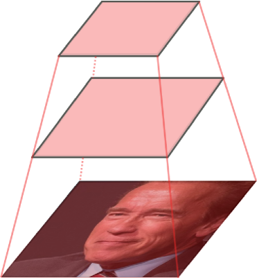
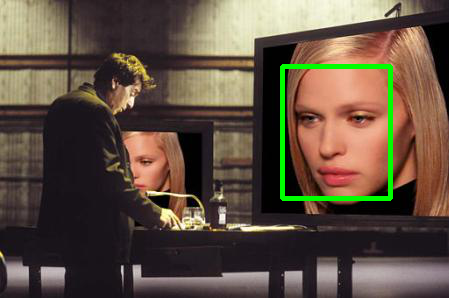
(a) Global loss layer.

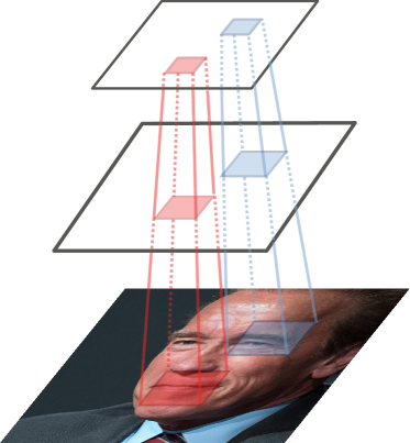
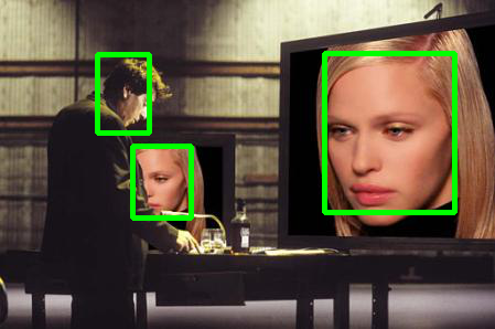
(b) Our grid loss layer.

Figure 1: Schematic overview of 1(a) standard global loss and 1(b) the proposed grid loss with an illustrative example on FDDB.

1 Introduction

We focus on single-class object detection and in particular address the problem of face detection. Several applications for face detection, such as surveillance or robotics, impose realtime requirements and rely on detectors which are fast, accurate and have low memory overhead. Traditionally, the most prominent approaches have been based on boosting [1, 2, 3, 4, 5, 6, 7] and Deformable Parts Models [8, 3]. More recently, following the success of deep learning for computer vision, e.g. [9], methods based on Convolutional Neural Networks have been applied to single-class object detection tasks, e.g. [10, 11, 12, 13].

One of the most challenging problems in the context of object detection is handling partial occlusions. Since the occluder might have arbitrary appearance, occluded objects have significant intra-class variation. Therefore, collecting large datasets capturing the huge variability of occluded objects, which is required for training large CNNs, is expensive. The main question we address in this paper is: How can we train a CNN to detect occluded objects?

In standard CNNs not every sub-part of the detection template is discriminative alone (i.e. able to distinguish faces from background), resulting in missed faces if parts of the detection template are occluded. Our main contribution is to address this issue by introducing a novel loss layer for CNNs, named grid loss, which is illustrated in Fig. 1. This layer divides the convolution layer into spatial blocks and optimizes the hinge loss on each of these blocks separately. This results in several independent detectors which are discriminative on their own. If one part of the window is occluded, only a subset of these detectors gets confused, whereas the remaining ones will still make correct predictions.

By requiring parts to be already discriminative on their own, we encourage the CNN to learn features suitable for classifying parts of an object. If we would train a loss over the full face, the CNN might solve this classification problem by just learning features which detect a subset of discriminative regions, e.g. eyes. We divide our window into sub-parts and some of these parts do not contain such highly prototypical regions. Thus, the CNN has to also learn discriminative representations for other parts corresponding to e.g. nose or mouth. We find that CNNs trained with grid loss develop more diverse and independent features compared to CNNs trained with a regular loss.

After training we map our grid loss layer back to a regular fully connected layer. Hence, no additional runtime cost is incurred by our method.

As we show in our experiments, grid loss significantly improves over using a regular linear layer on top of a convolution layer without imposing additional computational cost at runtime. We evaluate our method on publicly available face detection datasets [14, 15, 16] and show that it compares favorably to state-of-the-art methods. Additionally, we present a detailed parameter evaluation providing further insights into our method, which shows that grid loss especially benefits detection of occluded faces and reduces overfitting by efficiently combining several spatially independent detectors.

2 Related Work

Since there is a multitude of work in the area of face detection, a complete discussion of all papers is out of scope of this work. Hence, we focus our discussion only on seminal work and closely related approaches in the field and refer to [17] for a more complete survey.

A seminal work is the method of Viola and Jones [5]. They propose a realtime detector using a cascade of simple decision stumps. These classifiers are based on area-difference features computed over differently sized rectangles. To accelerate feature computation, they employ integral images for computing rectangular areas in constant time, independent of the rectangle size.

Modern boosting based detectors use linear classifiers on SURF based features [18], exemplars [19], and leverage landmark information with shape-indexed features for classification [20]. Other boosting based detectors compute integral images on oriented gradient features as well as LUV channels and use shallow boosted decision trees [3] or constrain the features on the feature channels to be block sized [21]. Additionally, [7] proposes CNN features for the boosting framework.

Another family of detectors are DPM [8] based detectors, which learn root and part templates. The responses of these templates are combined with a deformation model to compute a confidence score. Extensions to DPMs have been proposed which handle occlusions [22], improve runtime speed [23] and leverage manually annotated part positions in a tree structure [16].

Further, there are complimentary approaches improving existing detectors by domain adaption techniques [24]; and exemplar based methods using retrieval techniques to detect and align faces [25, 26].

Recently, CNNs became increasingly popular due to their success in recognition and detection problems, e.g. [27, 9]. They successively apply convolution filters followed by non-linear activation functions. Early work in this area applies a small number of convolution filters followed by sum or average pooling on the image [28, 29, 30]. More recent work leverages a larger number of filters which are pre-trained on large datasets, e.g. ILSVRC [31], and fine-tuned on face datasets. These approaches are capable of detecting faces in multiple orientations and poses, e.g. [10]. Furthermore, [12] uses a coarse-to-fine neural network cascade to efficiently detect faces in realtime. Successive networks in the cascade have a larger number of parameters and use previous features of the cascade as inputs. [32] propose a large dataset with attribute annotated faces to learn 5 face attribute CNNs for predicting hair, eye, nose, mouth and beard attributes (e.g. black hair vs. blond hair vs. bald hair). Classifier responses are used to re-rank object proposals, which are then classified by a CNN as face vs. non-face.

In contrast to recent CNN based approaches for face detection [32, 10, 12], we exploit the benefits of part-based models with our grid loss layer by efficiently combining several spatially independent networks to improve detection performance and increase robustness to partial occlusions. Compared to [32], our method does not require additional face-specific attribute annotations and is more generally applicable to other object detection problems. Furthermore, our method is suitable for realtime applications.

3 Grid Loss for CNNs

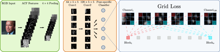
Figure 2: Overview of our method: our detection CNN builds upon Aggregate Channel Features (ACF) [2]. For each window, after pooling, we apply successive convolution filters to the input channels. To distinguish faces from non-faces we use pose-specific classifiers. Instead of minimizing the loss over the last full convolution map, we divide the map into small blocks and minimize a loss function on each of these blocks independently. We train our CNN end-to-end with backpropagation.

We design the architecture of our detector based on the following key requirements for holistic detectors: We want to achieve realtime performance to process video-stream data and achieve state-of-the-art accuracy. To this end, we use the network architecture as illustrated in Fig. 2. Our method detects faces using a sliding window, similar to [33]. We apply two convolution layers on top of the input features as detailed in Sec. 3.1. In Sec. 3.2, we introduce our grid loss layer to obtain highly accurate part-based pose-specific classifiers. Finally, in Sec. 3.3 we propose a regressor to refine face positions and skip several intermediate octave levels to improve runtime performance even further.

3.1 Neural Network Architecture

The architecture of our CNN consists of two $5\times 5$ convolution layers (see Fig. 2). Each convolution layer is followed by a Rectified Linear Unit (ReLU) activation. To normalize responses across layers, we use a Local Contrast Normalization (LCN) layer in between the two convolution layers. Further, we apply a small amount of dropout [34] of $0.1$ after the last convolution layer. We initialize the weights randomly with a Gaussian of zero mean and $0.01$ standard deviation. Each unit in the output layer corresponds to a specific face pose, which is trained discriminatively against the background class. We define the final confidence for a detection window as the maximum confidence over all output layer units.

In contrast to other CNN detectors, mainly for speed reasons, we use Aggregate Channel Features (ACF) [2] as low-level inputs to our network. For face detection we subsample the ACF pyramid by a factor of 4, reducing the computational cost of the successive convolution layers.

At runtime, we apply the CNN detector in a sliding window fashion densely over the feature pyramid at several scales. After detection, we perform Non Maxima Suppression (NMS) of two bounding boxes $B_{a}$ and $B_{b}$ using the overlap score $o_{\textrm{\tiny NMS}}(B_{a},B_{b})=\frac{\left|B_{a}\cap B_{b}\right|}{\min(\left|B_{a}\right|,\left|B_{b}\right|)}$, where $\left|B_{a}\cap B_{b}\right|$ denotes the area of intersection of the two boxes and $\min(\left|B_{a}\right|,\left|B_{b}\right|)$ denotes the minimum area of the two boxes. Boxes are suppressed if their overlap exceeds $0.3$, following [3].

(a) Regular loss

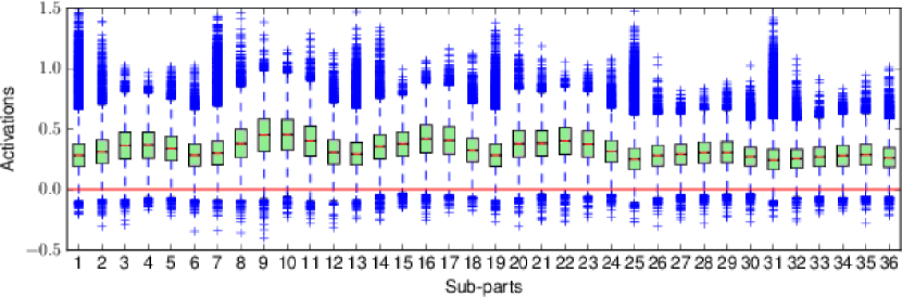
(b) Grid loss

Figure 3: Boxplot of $2\times 2$ part activations on the positive training set (i.e. by dividing the detection template into non-overlapping parts, as in Fig. 2). Activations trained by regular loss functions can have parts with negative median response. We mark parts whose 25% percentile is smaller than $0$ (red) and parts which have significant positive median activations compared to other parts (yellow).

3.2 Grid Loss Layer

CNN detection templates can have non-discriminative sub-parts, which produce negative median responses over the positive training set (see Fig. 3(a)). To achieve an overall positive prediction for a given positive training sample, they heavily rely on certain sub-parts of a feature map to make a strong positive prediction. However, if these parts are occluded, the prediction of the detector is negatively influenced. To tackle this problem, we propose to divide the convolution layers into small $n\times n$ blocks and optimize the hinge loss for each of these blocks separately. This results in a detector where sub-parts are discriminative (see Fig 3(b)). If a part of an input face is occluded, a subset of these detectors will still have non-occluded face parts as inputs. More formally, let $\boldsymbol{x}$ denote a vectorized $f\times r\times c$ dimensional tensor which represents the last convolution layer map, where $f$ denotes the number of filters, $r$ denotes the number of rows and $c$ the number of columns of the feature map. We divide $\boldsymbol{x}$ into small $f\times n\times n$ non-overlapping blocks $\boldsymbol{f}_{i}$, ${i=1\ldots N}$, with ${N=\lceil\frac{r}{n}\rceil\cdot\lceil\frac{c}{n}\rceil}$. To train our layer, we use the hinge loss

$$l(\boldsymbol{\theta})=\sum_{i=1}^{N}\max(0,m-y\cdot(\boldsymbol{w}_{i}^{\top}\boldsymbol{f}_{i}+b_{i})),$$ (1)

where $\boldsymbol{\theta}=[\boldsymbol{w}_{1},\boldsymbol{w}_{2},\ldots,\boldsymbol{w}_{N},b_{1},b_{2},\ldots,b_{N}]$, $m$ is the margin, $y\in\{-1,1\}$ denotes the class label, $\boldsymbol{w}_{i}$ and $b_{i}$ are the weight vector and bias for block $i$, respectively. In all our experiments we set $m$ to $\frac{1}{N}$, since each of the $N$ classifiers is responsible to push a given sample by $\frac{1}{N}$ farther away from the separating hyperplane.

Since some of the part classifiers might correspond to less discriminative face parts, we need to weight the outputs of different independent detectors correctly. Therefore, we combine this local per-block loss with a global hinge loss which shares parameters with the local classifiers. We concatenate the parameters $\boldsymbol{w}=[\boldsymbol{w}_{1},\boldsymbol{w}_{2},\ldots,\boldsymbol{w}_{N}]$ and set $b=\sum_{i}b_{i}$. Our final loss function is defined as

$$l(\boldsymbol{\theta})=\max(0,1-y\cdot(\boldsymbol{w}^{\top}\boldsymbol{x}+b))+\lambda\cdot\sum_{i=1}^{N}\max(0,m-y\cdot(\boldsymbol{w}_{i}^{\top}\boldsymbol{f}_{i}+b_{i})),$$ (2)

where $\lambda$ weights the individual part detectors vs. the holistic detector and is empirically set to $1$ in our experiments (see Sec. 4.3). To optimize this loss we use Stochastic Gradient Descent (SGD) with momentum. Since the weights $\boldsymbol{w}$ are shared between the global and local classifiers and $b$ is a sum of existing parameters, the number of additional parameters is only $N-1$ compared to a regular classification layer. However, at runtime no additional computational cost occurs, since we concatenate the local weight vectors to form a global weight vector and sum the local biases to obtain a global bias.

During training, the holistic loss backpropagates an error for misclassified samples to the hidden layers. Also, if certain parts are misclassifying a given sample, the part loss backpropagates an additional error signal to the hidden layers. However, for part detectors which are already discriminative enough to classify this sample correctly, no additional part error signal is backpropagated. In this way error signals of less discriminative parts are strengthened during training, encouraging the CNN to focus on making weak parts stronger rather than strengthening already discriminative parts (see Fig. 3(b)). This can also be observed when a sample is correctly classified by the holistic detector, but is misclassified by some part detectors. In this case only an error signal from the part classifiers is backpropagated, resulting in the part detectors becoming more discriminative. By training a CNN this way, the influence of several strong distinguished parts decreases, since they cannot backpropagate as many errors as non-discriminative parts, resulting in a more uniform activation pattern across parts, as seen in Fig. 3. With more uniform activations, even if some parts fail due to occlusions, the detector can recover. We experimentally confirm robustness to occlusions of our method in Sec. 4.4.

3.2.1 Regularization Effect.

Good features are highly discriminative and decorrelated, so that they are complementary if they are composed. Another benefit of grid loss is that it reduces correlation of feature maps compared to standard loss layers, which we experimentally show in Sec. 4.5. We accredit this to the fact that the loss encourages parts to be discriminative. For a holistic detector a CNN might rely on a few mid-level features to classify a window as face or background. In contrast to that, with grid loss the CNN has to learn mid-level features which can distinguish each face part from the background, resulting in a more diverse set of mid-level features. More diverse features result in activations which are decorrelated. Another interpretation of our method is, that we perform efficient model averaging of several part-based detectors with a shared feature representation, which reduces overfitting. We show in Sec. 4.6 that with a smaller training set size the performance difference to standard loss functions increases compared to grid loss.

3.2.2 Deeply Supervised Nets.

The output layer of a neural network has a higher chance of discriminating between background and foreground windows if its features are discriminative. Previous works [35, 19] improve the discriminativeness of their feature layers for object classification by applying a softmax or hinge loss on top of their hidden layers. Inspired by this success we replace the standard loss with our grid loss and apply it on top of our hidden layers. As our experiments show (Sec. 4.1), this further improves the performance without sacrificing speed, since these auxiliary loss layers are removed in the classification step.

3.3 Refinement of Detection Windows

Sliding window detectors can make mislocalization errors, causing high confidence predictions to miss the face by a small margin. This results in highly confident false positive predictions. To correct these errors, we apply a regressor to refine the location of the face. Further, we empirically observe that our CNN with the proposed grid loss is able to detect faces which are slightly smaller or bigger than the sliding window. Tree based detectors use an image pyramid with $8$ intermediate scales per octave. Applying several convolutions on top of all these scales is computationally expensive. Based on our observation, we propose to omit several of these intermediate scales and rely on the regressor to refine the face location. Details of this CNN are provided in the supplementary material.

Evaluation protocols for face detection use the PASCAL VOC overlap criterion to assess the performance. For two faces $F_{a}$ and $F_{b}$, the overlap $o_{\textrm{\tiny VOC}}$ is defined as

$$o_{\textrm{\tiny VOC}}(F_{a},F_{b})=\frac{\left|F_{a}\cap F_{b}\right|}{\left|F_{a}\cup F_{b}\right|},$$ (3)

where $\left|F_{a}\cap F_{b}\right|$ denotes the intersection and $\left|F_{a}\cup F_{b}\right|$ denotes the union of two face representations, i.e. ellipses or bounding boxes.

For ellipse predictions, the parameters major and minor axis length, center coordinates and orientation impact the PASCAL overlap criteria differently. For example, a difference of 1 radiant in orientation changes the overlap of two ellipses more than a change of 1 pixel in major axis length. To account for these differences, we compare minimizing the standard Sum of Squares Error (SSE) error with maximizing the PASCAL overlap criteria in Equation (3) directly. We compute the gradient entries $g_{i}$, $i=1,\ldots,5$, of the loss function numerically by central differences:

$$g_{i}(\boldsymbol{r})\approx\frac{o_{\textrm{\tiny VOC}}(\boldsymbol{r}+\epsilon_{i}\cdot\boldsymbol{a}_{i},\boldsymbol{y})-o_{\textrm{\tiny VOC}}(\boldsymbol{r}-\epsilon_{i}\cdot\boldsymbol{a}_{i},\boldsymbol{y})}{2\cdot\epsilon_{i}},$$ (4)

where $\boldsymbol{r}$ denotes the regressor predictions for the ellipse parameters, $\boldsymbol{y}$ denotes the ground truth parameters, $\boldsymbol{a}_{i}$ denotes the $i$-th standard basis vector where only the $i$-th entry is nonzero and set to $1$ and $\epsilon_{i}$ is the step size. Since the input size of this network is $40\times 40$ pixels, we use a patch size of $40\times 40$ pixels to rasterize both the ground truth ellipse and the predicted ellipse. Furthermore, we choose $\epsilon_{i}$ big enough so that the rasterization changes at least by one pixel.

4 Evaluation

We collect 15,106 samples from the Annotated Facial Landmarks in the Wild (AFLW) [36] dataset to train our detector on $80\times 80$ pixel windows in which $60\times 60$ faces are visible. Similar to [3], we group faces into 5 discrete poses by yaw angle and constrain faces to have pitch and roll between -22 and +22 degrees. Further following [3], we create rotated versions of each pose by rotating images by 35 degrees. We discard grayscale training images, since ACFs are color based. Finally, we mirror faces and add them to the appropriate pose-group to augment the dataset.

We set the ACF pre-smoothing radius to 1, the subsampling factor to 4 and the post-smoothing parameter to 0. Since we shrink the feature maps by a factor of 4, our CNN is trained on $20\times 20$ input patches consisting of 10 channels.

For training we first randomly subsample 10,000 negative examples from the non-person images of the PASCAL VOC dataset [37]. To estimate convergence of SGD in training, we use 20% of the data as validation set and the remaining 80% as training set. The detector is bootstrapped by collecting 10,000 negative patches in each bootstrapping iteration. After 3 iterations of bootstrapping, no hard negatives are detected.

Our regressor uses input patches of twice the size of our detector to capture finer details of the face. Since no post-smoothing is used, we reuse the feature pyramid of the detector and crop windows from one octave lower than they are detected.

We evaluate our method on three challenging public datasets: Face Detection Data Set and Benchmark (FDDB) [14], Annotated Faces in the Wild (AFW) [16] and PASCAL Faces [15]. FDDB consists of 2,845 images with 5,171 faces and uses ellipse annotations. PASCAL Faces is extracted from 851 PASCAL VOC images and has 1,635 faces and AFW consists of 205 images with 545 faces. Both AFW and PASCAL Faces use bounding box annotations.

4.1 Grid Loss Benefits

To show the effectiveness of our grid loss layer we run experiments on FDDB [14] using the neural network architecture described in Sec. 3.1 under the evaluation protocol described in [14]. For these experiments we do not use our regressor to exclude its influence on the results and apply the network densely across all 8 intermediate scales per octave (i.e. we do not perform layer skipping or location refinement). We compare standard logistic loss, hinge loss and our grid loss at a false positive count of 50, 100, 284 (which corresponds to $\approx$ 0.1 False Positives Per Image (FPPI)) and 500 samples. Further, during training we apply grid loss to our hidden layers to improve the discriminativeness of our feature maps. In Table 1 we see that our grid loss performs significantly better than standard hinge or logistic loss, improving true positive rate by 3.2% at 0.1 FPPI. Further, similar to the findings of [35, 19] our grid loss also benefits from auxiliary loss layers on top of hidden layers during training and additionally improves the true positive rate over the baseline by about 1%.

Method	50 FP	100 FP	284 FP	500 FP
L	0.776	0.795	0.817	0.824
H	0.758	0.786	0.819	0.831
G+L	0.803	0.827	0.851	0.859
G+H	0.807	0.834	0.851	0.858
G-h+L	0.809	0.836	0.862	0.869
G-h+H	0.815	0.838	0.863	0.871

Table 1: True positive rates of logistic (L), hinge (H), grid + logistic (G+L), grid + hinge (G+H), grid hidden + hinge (G-h+H) and grid hidden + logistic (G-h+L) loss functions on FDDB at a false positive (FP) count of 50, 100, 284 and 500. Best and second best results are highlighted.

4.2 Block Size

To evaluate the performance of our layer with regard to the block size, we train several models with different blocks of size $n=2^{\{1,2,3,4\}}$ in the output and hidden layer. We constrain the block size of the hidden layers to be the same as the block size of the output layers. Results are shown in Table 2. Our layer works best with small blocks of size 2 and degrades gracefully with larger blocks. In particular, if the size is increased to 16 the method corresponds to a standard CNN regularized with the method proposed in [35, 38] and thus, the grid loss layer does not show additional benefits.

Method	50 FP	100 FP	284 FP	500 FP
Block-2	0.815	0.838	0.863	0.871
Block-4	0.812	0.834	0.852	0.861
Block-8	0.790	0.809	0.830	0.838
Block-16	0.803	0.816	0.834	0.843

Table 2: Comparison of different block sizes on FDDB.

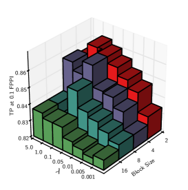
Figure 5: Evaluation of the weighting parameter $\lambda$.

4.3 Weighting Parameter

To evaluate the impact of the weighting parameter $\lambda$, we conduct experiments comparing the true positive rate of our method at a false positive count of 284 ($\approx$ 0.1 FPPI) with block sizes of $2^{\{1,2,3,4\}}$ and ${\lambda=\{5,1,0.1,0.05,0.01,0.005,0.001\}}$.

Fig. 5 shows that our method performs best with ${\lambda\approx 1}$ and smaller blocks of size 2 or 4. The performance of our method stays stable until $\lambda$ is varied more than one order of magnitude. As $\lambda$ decreases, the network converges to the performance of a regular CNN trained on hinge loss.

4.4 Robustness to Occlusions

To show that grid loss helps to detect faces with occlusions, we run an experiment on the Caltech Occluded Faces in the Wild (COFW) dataset [39]. The original purpose of the COFW dataset is to test facial landmark localization under occlusions. It consists of 1,852 faces with occlusion annotations for landmarks. We split the dataset into 329 heavily occluded faces with $\geq 30\%$ of all landmarks occluded (COFW-HO) and 1,523 less occluded faces (COFW-LO). Since this dataset is proposed for landmark localization, the images do not contain a large background variation.

For a fair evaluation, we measure the FPPI on FDDB, which has a more realistic background variation for the task of face detection. We report here the true positive rate on COFW at $0.1$ FPPI on FDDB. This evalution ensures that the detectors achieve a low false positive rate in a realistic detection setting and still detect occluded faces.

We evaluate both, the grid loss detector and the hinge loss detector on this dataset. The performance difference between these two detectors should increase on the occluded subset of COFW, since grid loss is beneficial for detecting occluded faces. In Table 4 we indeed observe that the performance difference on the heavily occluded subset significantly increases from 1.6% to 7% between the two detectors, demonstrating the favourable performance of grid loss for detecting occluded objects.

Method	COFW-HO	COFW-LO
G	0.979	0.998
H	0.909	0.982

Table 3: True Positive Rate on COFW Heavily Occluded (COFW-HO) and Less Occluded (LO) subsets with grid loss (G) and hinge loss (H).

Method	Correlation
Grid loss	225.96
Hinge loss	22500.25

Table 4: Grid loss reduces correlation in feature maps.

4.5 Effect on Correlation of Features

With grid loss we train several classifiers operating on spatially independent image parts simultaneously. During training CNNs develop discriminative features which are suitable to classify an image. By dividing the input image into several parts with different appearance, the CNN has to learn features suitable to classify each of these face parts individually.

Since parts which are located on the mouth-region of a face do not contain e.g. an eye, the CNN has to develop features to detect a mouth for this specific part detector. In contrast to that, with standard loss functions the CNN operates on the full detection window. To classify a given sample as positive, a CNN might solve this classification problem by just learning features which e.g. detect eyes. Hence, by operating on the full detection window, only a smaller set of mid-level features is required compared to CNNs trained on both, the full detection window and sub-parts.

Therefore, with our method, we encourage CNNs to learn more diverse features. More diverse features result in less correlated feature activations, since for a given sample different feature channels should be active for different mid-level features. To measure this, we train a CNN with and without grid loss. For all spatial coordinates of the last $12\times 12$ convolution layer, we compute a $128\times 128$ dimensional normalized correlation matrix. We sum the absolute values of the off-diagonal elements of the correlation matrices. A higher number indicates more correlated features and is less desirable. As we see in Table 4 our grid loss detector learns significantly less correlated features.

4.6 Training Set Size

Regularization methods should improve performance of machine learning methods especially when the available training data set is small. The performance gap between a method without regularization to a method with regularization should increase with a smaller amount of training data. To test the effectiveness of our grid loss as regularization method, we subsample the positive training samples by a factor of 0.75 - 0.01 and compare the performance to a standard CNN trained on hinge loss, a CNN trained with hinge loss on both the output and hidden layers [35, 38], and a CNN where we apply grid loss on both hidden layers and the output layer. To assess the performance of each model, we compare the true positive rate at a false positive count of 284 ($\approx$ 0.1 FPPI). In Table 5 we see that our grid loss indeed acts as a regularizer. The performance gap between our method and standard CNNs increases from 3.2% to 10.2% as the training set gets smaller. Further, we observe that grid loss benefits from the method of [35, 38], since by applying grid loss on top of the hidden layers, the performance gap increases even more.

M	1.00	0.75	0.50	0.25	0.10	0.05	0.01
G-h	0.863	0.858	0.856	0.848	0.841	0.833	0.802
G	0.851	0.849	0.848	0.844	0.835	0.812	0.802
H-h	0.834	0.817	0.813	0.801	0.786	0.769	0.730
H	0.819	0.799	0.795	0.770	0.761	0.747	0.700

Table 5: Impact of training on a sub-set (i.e. 0.75 - 0.01) of the positive training set on FDDB at 0.1 FPPI using the hinge loss (H), hinge loss on hidden layers (H-h) and our grid loss (G) and grid loss on hidden layers (G-h).

4.7 Ellipse Regressor and Layer Skipping

We compare the impact of an ellipse regressor trained on the PASCAL overlap criterion with a regressor trained on the SSE loss. We evaluate the impact on the FDDB dataset using the continuous evaluation protocol [14], which weighs matches of ground truth and prediction with their soft PASCAL overlap score. In Table 6 we see that minimizing the numerical overlap performs barely better than minimizing the SSE loss in the parameter space (i.e. 0.1% to 0.2%). We hypothesize that this is caused by inconsistent annotations in our training set.

Further, we compare our model with and without an ellipse regressor using different image pyramid sizes. We evaluate the performance on the FDDB dataset under the discrete evaluation protocol. In Table 7 we see that regressing ellipses improves the true positive rate by about 1%. But more importantly, using a regressor to refine the face positions allows us to use fewer intermediate scales in our image pyramid without significant loss in accuracy. This greatly improves runtime performance of our detector by a factor of 3-4 (see Sec. 4.10).

Method	50 FP	100 FP	284 FP	500 FP	1000 FP
NUM (D)	0.680	0.690	0.702	0.708	0.714
SSE (D)	0.679	0.688	0.700	0.706	0.713

Table 6: Continuous evaluation of the two proposed ellipse loss functions: Numerical PASCAL VOC overlap (NUM) and SSE on FDDB.

Method	50 FP	100 FP	284 FP	500 FP
NUM (D)	0.843	0.857	0.872	0.879
NUM (S)	0.835	0.851	0.867	0.874
SSE (D)	0.844	0.857	0.872	0.878
SSE (S)	0.835	0.848	0.866	0.873
w/o (D)	0.815	0.838	0.863	0.871

Table 7: Effect of numerical loss (NUM), SSE loss (SSE) and no ellipse regressor (w/o) applied densely (D) on all pyramid levels or skipping (S) layers on FDDB.

4.8 Building a Highly Accurate Detector

Grid loss can also be used to improve the detection performance of deeper networks, yielding highly accurate detections. To this end, following [40], we replace each $5\times 5$ convolution layer with two $3\times 3$ layers, doubling the number of layers from $2$ to $4$. After the first convolution layer we apply LCN. Further, we increase the number of convolution filters in our layers to $64$, $256$, $512$ and $512$, respectively. We denote this detector Big in the following experiments.

4.9 Comparison to the State-of-the-Art

We compare our detector to the state-of-the-art on the FDDB dataset [14], the AFW dataset [16] and PASCAL Faces dataset [15], see Figs. 9, 9 and 10. For evaluation on AFW and PASCAL Faces we use the evaluation toolbox provided by [3]. For evaluation on FDDB we use the original evaluation tool provided by [14]. We report the accuracy of our small fast model and our large model. On FDDB our fast network combined with our regressor retrieves 86.7% of all faces at a false positive count of 284, which corresponds to about 0.1 FPPI on this dataset. With our larger model we can improve the true positive rate to 89.4% at 0.1 FPPI, outperforming the state-of-the-art by 0.7%. In our supplementary material we show that when we combine AlexNet with our method, we can increase the true positive rate to 90.1%. On PASCAL Faces and AFW we outperform the state-of-the-art by $1.38\%$ and $1.45\%$ Average Precision respectively.

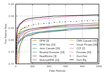
Figure 8: Discrete evaluation on the FDDB [14] dataset.

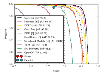
Figure 9: Evaluation on the PASCAL Faces [15] dataset.

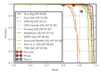
Figure 10: Our method outperforms state-of-the-art methods on AFW [16].

4.10 Computational Efficiency

We implemented our method with Theano [41] and Python and ran our experiments on a desktop machine with a NVIDIA GTX 770 and a 3.20 GHz Intel Core i5 CPU. Our small dense model needs about 200 ms (GPU) to run on images with a size of $640\times 480$ pixels. With skipping intermediate scales our network runs in about 50 ms (GPU) on the same computer using non-optimized Python code. On the CPU our small network runs in about 170 ms with layer skipping, achieving competitive runtime performance compared to fast tree based methods, e.g. [3, 21], while outperforming them in accuracy. Note that we do not rely on speedup techniques such as image patchwork [42, 43], decomposing convolution filters into separable kernels [44, 45], or cascades [12]. Combining our method with these approaches can improve the runtime performance even more.

5 Conclusion

We presented a novel loss layer named grid loss, which improves the detection accuracy compared to regular loss layers by dividing the last convolution layer into several part detectors. This results in a detector which is more robust to occlusions compared to standard CNNs, since each detector is encouraged to be discriminative on its own. Further, in our evaluation we observe that CNNs trained with grid loss develop less correlated features and that grid loss reduces overfitting. Our method does not add any additional overhead during runtime. We evaluated our detector on face detection tasks and showed that we outperform competing methods on FDDB, PASCAL Faces and AFW. The fast version of our method runs at 20 FPS on standard desktop hardware without relying on recently proposed speedup mechanisms, while achieving competitive performance to state-of-the-art methods. Our accurate model outperforms state-of-the-art methods on public datasets while using a smaller amount of parameters. Finally, our method is complementary to other proposed methods, such as the CNN cascade [12] and can improve the discriminativeness of their feature maps.

Acknowledgements

This work was supported by the Austrian Research Promotion Agency (FFG) project DIANGO (840824).

References

- [1] Benenson, R., Mathias, M., Tuytelaars, T., Van Gool, L.: Seeking the Strongest Rigid Detector. In: Proc. CVPR. (2013)
- [2] Dollár, P., Appel, R., Belongie, S., Perona, P.: Fast Feature Pyramids for Object Detection. PAMI 36(8) (2014) 1532–1545
- [3] Mathias, M., Benenson, R., Pedersoli, M., Van Gool, L.: Face Detection without Bells and Whistles. In: Proc. ECCV. (2014)
- [4] Schulter, S., Leistner, C., Wohlhart, P., Roth, P.M., Bischof, H.: Accurate Object Detection with Joint Classification-Regression Random Forests. In: Proc. CVPR. (2014)
- [5] Viola, P., Jones, M.J.: Robust Real-Time Face Detection. IJCV 57(2) (2004) 137–154
- [6] Zhang, S., Benenson, R., Schiele, B.: Filtered Channel Features for Pedestrian Detection. In: Proc. CVPR. (2015)
- [7] Yang, B., Yan, J., Lei, Z., Li, S.Z.: Convolutional Channel Features. In: Proc. ICCV. (2015)
- [8] Felzenszwalb, P.F., Girshick, R.B., McAllester, D., Ramanan, D.: Object Detection with Discriminatively Trained Part-Based Models. PAMI 32(9) (2010) 1627–1645
- [9] Krizhevsky, A., Sutskever, I., Hinton, G.E.: ImageNet Classification with Deep Convolutional Neural Networks. In: NIPS. (2012)
- [10] Farfade, S.S., Saberian, M., Li, L.J.: Multi-view Face Detection Using Deep Convolutional Neural Networks. In: Proc. ICMR. (2015)
- [11] Hosang, J., Omran, M., Benenson, R., Schiele, B.: Taking a Deeper Look at Pedestrians. In: Proc. CVPR. (2015)
- [12] Li, H., Lin, Z., Shen, X., Brandt, J., Hua, G.: A Convolutional Neural Network Cascade for Face Detection. In: Proc. CVPR. (2015)
- [13] Sermanet, P., Kavukcuoglu, K., Chintala, S., LeCun, Y.: Pedestrian Detection with Unsupervised Multi-Stage Feature Learning. In: Proc. CVPR. (2013)
- [14] Jain, V., Learned-Miller, E.: FDDB: A Benchmark for Face Detection in Unconstrained Settings. Technical Report UM-CS-2010-009, University of Massachusetts, Amherst (2010)
- [15] Yan, J., Zhang, X., Lei, Z., Li, S.Z.: Face Detection by Structural Models. IVC 32(10) (2014) 790 – 799
- [16] Zhu, X., Ramanan, D.: Face Detection, Pose Estimation and Landmark Estimation in the Wild. In: Proc. CVPR. (2012)
- [17] Zafeiriou, S., Zhang, C., Zhang, Z.: A Survey on Face Detection in the Wild: Past, Present and Future. CVIU 138 (2015) 1–24
- [18] Li, J., Zhang, Y.: Learning Surf Cascade for Fast and Accurate Object Detection. In: Proc. CVPR. (2013)
- [19] Li, H., Lin, Z., Brandt, J., Shen, X., Hua, G.: Efficient Boosted Exemplar-Based Face Detection. In: Proc. CVPR. (2014)
- [20] Chen, D., Ren, S., Wei, Y., Cao, X., Sun, J.: Joint Cascade Face Detection and Alignment. In: Proc. ECCV. (2014)
- [21] Yang, B., Yan, J., Lei, Z., Li, S.Z.: Aggregate Channel Features for Multi-View Face Detection. In: Proc. IJCB. (2014)
- [22] Ghiasi, G., Fowlkes, C.C.: Occlusion Coherence: Localizing Occluded Faces with a Hierarchical Deformable Part Model. In: Proc. CVPR. (2014)
- [23] Yan, J., Lei, Z., Wen, L., Li, S.: The Fastest Deformable Part Model for Object Detection. In: Proc. CVPR. (2014)
- [24] Li, H., Hua, G., Lin, Z., Brandt, J., Yang, J.: Probabilistic Elastic Part Model for Unsupervised Face Detector Adaptation. In: Proc. ICCV. (2013)
- [25] Shen, X., Lin, Z., Brandt, J., Wu, Y.: Detecting and Aligning Faces by Image Retrieval. In: Proc. CVPR. (2013)
- [26] Kumar, V., Namboodiri, A.M., Jawahar, C.V.: Visual Phrases for Exemplar Face Detection. In: Proc. ICCV. (2015)
- [27] Girshick, R., Donahue, J., Darrell, T., Malik, J.: Rich Feature Hierarchies for Accurate Object Detection and Semantic Segmentation. In: Proc. CVPR. (2014)
- [28] Garcia, C., Delakis, M.: Convolutional Face Finder: A Neural Architecture for Fast and Robust Face Detection. PAMI 26(11) (2004) 1408–1423
- [29] Rowley, H., Baluja, S., Kanade, T., et al.: Neural Network-Based Face Detection. PAMI 20(1) (1998) 23–38
- [30] Vaillant, R., Monrocq, C., LeCun, Y.: Original Approach for the Localisation of Objects in Images. IEEE Proceedings of Vision, Image and Signal Processing 141(4) (1994) 245–250
- [31] Russakovsky, O., Deng, J., Su, H., Krause, J., Satheesh, S., Ma, S., Huang, Z., Karpathy, A., Khosla, A., Bernstein, M., Berg, A.C., Fei-Fei, L.: ImageNet Large Scale Visual Recognition Challenge. IJCV (2015) 1–42
- [32] Yang, S., Luo, P., Loy, C.C., Tang, X.: From Facial Parts Responses to Face Detection: A Deep Learning Approach. In: Proc. ICCV. (2015)
- [33] Sermanet, P., Eigen, D., Zhang, X., Mathieu, M., Fergus, R., LeCun, Y.: OverFeat: Integrated Recognition, Localization and Detection using Convolutional Networks. In: Proc. ICLR. (2014)
- [34] Srivastava, N., Hinton, G., Krizhevsky, A., Sutskever, I., Salakhutdinov, R.: Dropout: A Simple Way to Prevent Neural Networks from Overfitting. JMLR 15(1) (2014) 1929–1958
- [35] Szegedy, C., Liu, W., Jia, Y., Sermanet, P., Reed, S., Anguelov, D., Erhan, D., Vanhoucke, V., Rabinovich, A.: Going Deeper with Convolutions. In: Proc. CVPR. (2015)
- [36] Köstinger, M., Wohlhart, P., Roth, P.M., Bischof, H.: Annotated Facial Landmarks in the Wild: A Large-scale, Real-world Database for Facial Landmark Localization. In: Proc. BeFIT (in conj. with ICCV). (2011)
- [37] Everingham, M., Eslami, S.M.A., Van Gool, L., Williams, C.K.I., Winn, J., Zisserman, A.: The Pascal Visual Object Classes Challenge: A Retrospective. IJCV 111(1) (2015) 98–136
- [38] Lee, C.Y., Xie, S., Gallagher, P., Zhang, Z., Tu, Z.: Deeply-Supervised Nets. In: Proc. AISTATS. (2015)
- [39] Burgos-Artizzu, X., Perona, P., Dollár, P.: Robust face landmark estimation under occlusion. In: Proc. ICCV. (2013)
- [40] Simonyan, K., Zisserman, A.: Very Deep Convolutional Networks for Large-Scale Image Recognition. In: Proc. ICLR. (2015)
- [41] Bastien, F., Lamblin, P., Pascanu, R., Bergstra, J., Goodfellow, I.J., Bergeron, A., Bouchard, N., Bengio, Y.: Theano: New Features and Speed Improvements. In: Proc. NIPS Deep Learning Workshop. (2012)
- [42] Dubout, C., Fleuret, F.: Exact Acceleration of Linear Object Detectors. In: Proc. ECCV. (2012)
- [43] Girshick, R., Iandola, F., Darrell, T., Malik, J.: Deformable Part Models are Convolutional Neural Networks. In: Proc. CVPR. (2015)
- [44] Jaderberg, M., Vedaldi, A., Zisserman, A.: Speeding up Convolutional Neural Networks with Low Rank Expansions. In: Proc. BMVC. (2014)
- [45] Zhang, X., Zou, J., He, K., Sun, J.: Accelerating Very Deep Convolutional Networks for Classification and Detection. arXiv abs/1505.06798 (2015)