A Likelihood Ratio Detector for Identifying Within-Perimeter Computer Network Attacks.

Abstract

The rapid detection of attackers within firewalls of enterprise computer networks is of paramount importance. Anomaly detectors address this problem by quantifying deviations from baseline statistical models of normal network behavior and signaling an intrusion when the observed data deviates significantly from the baseline model. However, many anomaly detectors do not take into account plausible attacker behavior. As a result, anomaly detectors are prone to a large number of false positives due to unusual but benign activity. This paper first introduces a stochastic model of attacker behavior which is motivated by real world attacker traversal. Then, we develop a likelihood ratio detector that compares the probability of observed network behavior under normal conditions against the case when an attacker has possibly compromised a subset of hosts within the network. Since the likelihood ratio detector requires integrating over the time each host becomes compromised, we illustrate how to use Monte Carlo methods to compute the requisite integral. We then present Receiver Operating Characteristic (ROC) curves for various network parameterizations that show for any rate of true positives, the rate of false positives for the likelihood ratio detector is no higher than that of a simple anomaly detector and is often lower. We conclude by demonstrating the superiority of the proposed likelihood ratio detector when the network topologies and parameterizations are extracted from real-world networks.

1 Introduction

Many existing systems designed to detect intrusions into computer networks monitor data streams only at the perimeter of the network. In addition, many network intrusion detection systems, such as snort  (Roesch et al.,, 1999), are signature based, meaning that every communication entering or leaving the network is examined for matches to a database of signatures, or indicators of compromise. At this point, the long list of breaches to corporate networks (Krebs,, 2014, 2015) speaks loudly to the insufficiency of these methods. Attackers are able to innovate rapidly in order to avoid signature schemes, and penetrate these perimeter systems seemingly at will. Therefore, there is a pressing need to identify attackers within network perimeters, and to do so using behavioral methods rather than signatures.

Anomaly detectors — a model-based approach— show promise in detecting within-perimeter attacks. In general, anomaly detectors quantify “normal” network behavior, and when observed behavior significantly deviates from the baseline model, an intrusion is signaled. As a simple example, consider an anomaly detector that models a computer network as a directed graph where nodes are users within a network and edges represent a communication channel between users. The detector is then calibrated such that it specifies the average rate of packet transfer along each edge. When the observed rate of packet transfers is sufficiently different from the calibrated rate of packet transfers, the detector signals an intrusion.

In practice, many reported anomalies end up being false, reflecting behavior that is unusual but benign. This is due in part to an incomplete specification of normal network behavior in the null hypothesis as well as the difficulty in modeling and predicting the behavior of humans that interact over the network. There are at least two approaches in addressing this issue. The first is to improve the specification of the network under normal conditions. The second is to develop a model of attacker behavior and compare the probability of the observed behavior under the hypothesis that the network has been compromised against the hypothesis that the network is functioning under normal conditions. With an accurately specified attacker model, such an approach would rule out benign but unusual activity as being malicious since it is not consistent with attacker behavior. Our work in this paper takes the second approach. More explicitly, to our knowledge this paper is the first to incorporate an exact parametric specification of attacker behavior into a likelihood ratio detector for identifying malicious traversal activity within a network perimeter.

The challenge is in how to model the behavior of a network that has been penetrated without pre-supposing attacker methods, since these methods evolve rapidly. To see how this might be done, consider a common attack conducted on an enterprise network. First, a Phishing email or set of emails, containing either a malicious attachment or a link to an internet host serving malware, is sent to the target network. Click rates on Phishing emails, even after enterprise training is conducted, can be as high as 50% (Kumaraguru et al.,, 2009), providing a high-confidence intrusion vector.

At this point, the firewall is penetrated and the attacker has control of an initial host in the target network. The attack is far from complete since the initially compromised host is not the primary target of the attacker. Instead, the attacker seeks to penetrate the network and access key servers. However, since credentials are typically required to access these servers, the attacker undergoes a process known as lateral movement to move among hosts collecting these credentials (Kent and Liebrock,, 2013). This means that there is a definite sequence in the movement of the attacker across the network, from computers with low value (for any of the goals of inserting malware, extracting data, or stealing credentials) to computers with higher value, such as data servers and active directories. This will be true no matter what precise methods the attacker uses to achieve that movement. As a result, the attacker’s traversal will leave a trace of increasing network traffic going from low value computers to progressively higher value ones. Therefore, an increase in network traffic along paths from low value to high value nodes in a network can be used as the basis of a model of network behavior once it has been penetrated.

The approach in this paper is parallel to that of Jiang et al., 2014a in that we first propose a model of attacker behavior and a novel detection criteria based on a likelihood ratio. For various network parameterizations, we simulate network activity in both the normal and compromised state. We then employ receiver operating characteristic (ROC) curves to show that the proposed likelihood ratio detector outperforms a simple anomaly detector that does not exploit information regarding the traversing nature of an attack. In addition we develop the Monte Carlo techniques used to approximate the relevant integrals in computing our proposed likelihood ratio. Finally, we extract topologies and parameter data from real-world networks and then simulate attacker behavior. The results show that in real-world networks, our proposed likelihood ratio detector is superior to the simple anomaly detector.

2 Background

Model-based anomaly detection proceeds by modeling and estimating the parameters, $\hat{\theta}$, of a computer network under normal conditions. Next, given a dataset $\mathbf{D}$ under question, the likelihood of the parameters given the data can be evaluated: $\mathcal{L}(\mathbf{\hat{\theta}}\mid\mathbf{D})$. A generalized likelihood ratio test (GLRT) can then be used to infer whether a more likely alternative parameterization is present given data $\mathbf{D}$

$$GLRT=\frac{\mathcal{L}(\mathbf{\hat{\theta}}\mid\mathbf{D})}{\sup_{\mathbf{\theta}\in\mathbf{\Theta}}\mathcal{L}(\mathbf{\theta}\mid\mathbf{D})}$$

where $\mathbf{\Theta}$ is an alternative parameter space. Typically, we choose what data $\mathbf{D}$ to collect in order to facilitate statistical discovery of security breaches. For example, the network model under normal conditions might be a graph connecting computers (nodes or hosts) with edges representing parameterized time-series of traffic. The data collected would then be communications between nodes. When the observed communication pattern is different from the parameterized time-series, the anomaly detector would sound an alarm. Additionally, since attacks typically cover multiple nodes and edges, subgraphs can be used to group data from multiple nodes and edges into $\mathbf{D}$ for increased detection power. Such graph based methods include Borgwardt et al., (2006); Eberle et al., (2010); Neil et al., (2013); Staniford-Chen et al., (1996); Djidjev et al., (2011).

If we know that the attacker behaves according to a specified alternative parameter vector, say $\bf\theta_{A}$, then the uniformly most powerful test for rejecting the null hypothesis that no attack is present is a likelihood ratio test where $\bf{\theta}_{A}$ is used in the denominator. That is, if we know the attacker is behaving according to $\bf{\theta}_{A}$, the power of the test is maximized when using the test statistic

$$\overline{GLRT}=\frac{\mathcal{L}(\mathbf{\hat{\theta}}\mid\mathbf{D})}{\mathcal{L}(\mathbf{\theta_{A}}\mid\mathbf{D})}.$$ (1)

However, the set of alternatives $\mathbf{\Theta}$ is typically under-specified. In other words, anomaly detectors do not specify exact attacker behavior but simply restrict the parameter space of alternatives. A representative example of such a detector is the Modeled Attack Detector (MAD) given in Thatte et al., (2008). In their work, the authors consider the rate of incoming traffic in order to detect a Distributed Denial of Service (DDoS) attack. They assume that that under normal conditions, the number of incoming connections can be modeled by a Poisson distribution with average rate of messages per unit time of $\lambda_{B}$. The authors treat $\lambda_{B}$ as a known and calibrated parameter. Therefore, given a sequence of incoming connections (i.e. one unit of network traffic) $\mathbf{D}=\{d_{1},d_{2}...d_{N}\}$ per unit time interval, the probability of observing $\mathbf{D}$ under the hypothesis that $H_{0}$ = no attack is taking place is given by

$$P(\mathbf{D}|H_{0})=\prod_{i=1}^{N}\frac{e^{-\lambda_{B}}\lambda_{B}^{d_{i}}}{d_{i}!}.$$ (2)

The authors assume that under a DDoS attack the network receives additional malicious connections at fixed, deterministic time intervals but at an unknown rate. If the rate was known, the probability of an observed sequence under the hypothesis that $H_{1}$ = DDoS attack is occurring is given by

$$P(\mathbf{D}|H_{1})=\prod_{i=1}^{N}\frac{\lambda_{B}^{d_{i}-\lambda_{m}}e^{-\lambda_{B}}}{(d_{i}-\lambda_{m})!}.$$ (3)

where $\lambda_{m}$ is the rate at which the network receives malicious connections. In reality, $\lambda_{m}$—the rate under the alternative hypothesis—is unknown so a simple likelihood ratio test is unavailable. Instead, the authors employ a GLRT which is given by

$$LR=\frac{P(\mathbf{D}|H_{0})}{\displaystyle\max_{\lambda_{m}}P(\mathbf{D}|H_{1})}$$ (4)

where the denominator is maximized when $\lambda_{m}=-\lambda_{B}+\frac{1}{N}\sum_{i=1}^{N}d_{i}$. When $LR$ is less than a predefined threshold, the MAD indicates an attack.

Although the model of Thatte et al., (2008) is concerned with DDoS attacks and not within-perimeter attacks, it succinctly showcases the key elements of anomaly detection that this paper intends to improve upon. Like the MAD, the work presented in this paper will use a likelihood ratio as the detection criteria. However, unlike the MAD, this paper will focus on incorporating exact specification of attacker behavior into a likelihood ratio detector for within-perimeter detection to improve detection accuracy.

The likelihood ratio detector we introduce in this paper is most similar to the anomaly detector presented in Neil et al., (2013), known as PathScan. In that work, communication channels between hosts are in either an active or inactive state. In the active state, it is assumed that communications take place stochastically at a known rate. In the inactive state, no communication occurs. The anomaly detector does not observe the state of the edge but instead only knows the probability of an edge transitioning (transition parameter) between the active and inactive states and observes communications between hosts during a moving time window. “Attacker behavior” is modeled as an increase in the probability of an edge transitioning from an inactive to an active state. The authors then compute the probability of an observed dataset under the hypothesis that the transition parameter is equal to the calibrated transition parameter and compare that likelihood to the likelihood under the maximum likelihood estimate of the transition parameter. When the value of the likelihood at the maximum likelihood estimate is sufficiently different from the value of the likelihood under the calibrated transition parameter, PathScan indicates an intrusion. Our novel detector presented below is similar to PathScan in that it uses a likelihood ratio to detect within perimeter anomalies. However, our detector is different from PathScan in that it explicitly captures the the fact that the attacker must traverse the network when attempting to access key information located on various nodes in the network. Furthermore, our work shows how to incorporate exact information of an attacker’s strategy into the likelihood ratio.

It is important to note that likelihood and likelihood ratio based approaches are not the only characterizations of model-based anomaly detectors. For example, Lee and Xiang, (2001) focuses on information theoretic measures for anomaly detection such as entropy, conditional entropy, relative conditional entropy, information gain, and information cost. From a learning-based approach, Ryan et al., (1998) uses artificial neural networks with supervised learning, based on the back-propagation neural network, called Neural Network Intrusion Detector. However, the limitations to supervised learning as applied to intrusion detection are well documented and are discussed in Sommer and Paxson, (2010).

A sizable portion of the literature approaches anomaly detection from the frequency domain. The work of Jiang et al., 2015b uses principal component analysis on wavelet transforms of network traffic to detect anomalies in backbone networks. Similarly, the work of Jiang et al., 2014a uses the $S$-transform to convert network traffic data into the frequency domain and then presents ROC curves that illustrate the effectiveness of their approach.

Another approach to anomaly detection is through the use of sequential hypothesis tests. In a sequential hypothesis test, the test is applied multiple times as the data are generated. Data that are included in the first hypothesis test can be included in hypothesis tests later in time. Two examples of sequential based hypothesis tests are Wang et al., (2004) and Kang et al., (2009), who employ CUSUM charts to determine when the parameters that govern network behavior (such as packet transfer rates between hosts) have changed, which signals a potential intrusion.

To pinpoint our work in the current literature, we note that our proposed likelihood ratio detector can be classified as a within-perimeter (like PathScan), likelihood ratio-based (like Thatte et al., (2008)) network intrusion detector. The analysis is performed in the time domain (like Thatte et al., (2008) and Neil et al., (2013)). It does not use sequential hypothesis tests (as in Kang et al., (2009)), supervised learning (as in Ryan et al., (1998)) or information theoretic quantities (as in Lee and Xiang, (2001)). Additionally, our work enhances the current state of the art likelihood ratio intrusion detection systems in that it shows how to incorporate explicit traversal behavior into the denominator of the likelihood ratio. For a more detailed survey of general anomaly detection, see the surveys of Chandola et al., (2009), Lee and Stolfo, (2000), Garcia-Teodoro et al., (2009) and Kantas et al., (2009).

3 Model

We model a computer network as a directed graph, potentially with cycles, where each node (also referred to as “host”) represents a computer or a human inside the firewall. Each node has an associated state. Examples of human nodes are users, system administrators, and hackers, whose states can represent their knowledge, their strategies, etc. Each directed edge represents a potential communication directly connecting one node (human or computer) to another node (human or computer). These edges have associated states, which represent communication messages. So the computer network evolves according to a Markov process across all possible joint states of every node and every edge.

In this initial project, we only consider computer nodes, treating the human using a particular computer as part of that computer. We also only consider those computers that are inside the firewall. Each node can be in one of two states, “normal” or “compromised”. Similarly, each edge can be in one of two states, “no message”, or “message in transit”. When a node is in a normal state, it sends benign messagesalong any of its directed edges according to an underlying Poisson process with a pre-specified rate. To maintain generality, we do not define a message explicitly but only suggest that a message can be, among many other alternatives, a remote desktop protocol connection or file transfer protocol connection. When a node is compromised, it still sends benign messages at the same rate as when it is not compromised, but now it superimposes malicious messages. These are generated according to another Poisson process, with a much lower rate, thus effectively increasing the Poisson rate for message emissions out of a compromised node by a small amount. We use a stochastic model of attacker behavior because in reality, it is impossible to perfectly predict each action of the attacker. In other words, we are not claiming that attackers are strategically randomizing their actions. Instead, all we are claiming is that the only information afforded to the detectors is that the attacker’s behavior —strategic or otherwise— can be described by a Poisson process. The task of network defense is to detect the small increases in the message transmission rates and decide whether they fall into a pattern indicative of attack.

For simplicity we assume that if an edge from a compromised node to a non-compromised node gains a new malicious message at time $t$, then with probability $1.0$ the second node becomes compromised and the new malicious message disappears immediately, leaving a trace on our net-monitoring equipment that that message traveled down that edge at $t$. No node can become compromised spontaneously, and no node can become uncompromised.

3.1 Definitions

Let $G=(V,E)$ be the directed graph of a computer network where $V=\{v_{1},v_{2}...v_{N}\}$ is the set of nodes and $E$ is a set of directed edges that represent communication channels between nodes. Let $\sigma\in{\mathbb{B}}^{N}$ denote the state of all nodes in the network and $\sigma_{v_{i}}$ denote the state of node $v_{i}$: $1$ representing the uncompromised state and $0$ representing the compromised state. The Markov process governing the computer network is parameterized by the set of Poisson rates $\lambda\equiv\{(\lambda_{v,v^{\prime},\sigma_{v}}):v,v^{\prime}\in V,v^{\prime}\neq v,\sigma_{v}\in{\mathbb{B}}\}$ giving the total rate at which $v$ sends messages to $v^{\prime}$ when $v$ is in state $\sigma_{v}$. We write the rate parameter for just emission of malicious message from $v$ to $v^{\prime}$ as $\Delta_{v,v^{\prime}}\equiv\lambda_{v,v^{\prime},0}-\lambda_{v,v^{\prime},1}$. A directed edge from $v$ to $v^{\prime}$ exists if and only if $\lambda_{v,v^{\prime},s}>0$ for some $s\in\sigma_{v}$.

Suppose we observe the traffic on a net for a time interval $[0,T]$, and denote by $(\tau,v,v^{\prime})$ an observation that a message was added at time $\tau$ to the edge from $v$ to $v^{\prime}$. The resulting dataset $D=\{(\tau_{i},v_{i},v^{\prime}_{i})\}$, has $\tau_{i}\in[0,T]$ and each $(v_{i},v^{\prime}_{i})\in V^{2}$. We assume that the observation process is noise-free, i.e., that all messages are recorded and no spurious messages are.

In time continuous processes like this, the probability that two nodes get compromised at exactly the same time is precisely zero; as a result, we can assume a strict time ordering among the compromised nodes. For all $1\leq k\leq N$ indicating the possible number of node compromises that occur in $[0,T]$ (though others might occur later), define ${\mathbb{S}}^{k}$ as the set of vectors $s\in V^{k}$ such that each element of ${\mathbb{S}}^{k}$ uniquely defines an ordering of $k$ nodes that can become compromised when the network perimeter has been penetrate. Define ${\mathbb{S}}=\cup_{k=1}^{N}{\mathbb{S}}^{k}$. Also define the space $Z\equiv[0,T]\cup\{*\}$, whose elements are either a time of compromise in the observation window $[0,T]$, or a $*$ to indicate no compromise occurs in that interval. We will mostly consider vectors $z=(z_{v_{1}},z_{v_{2}},...z_{v_{m}})\in Z^{m}$ specifying the times of compromise of various nodes, and index components of the vectors $z$ by the nodes compromised (or not for $*$) at those times. So $z_{s_{i}}$ is the time that $s_{i}$, the $i$’th node to get compromised, gets compromised, or is a $*$.

For each pair $(v,v^{\prime})$, it will be useful to define an associated function $\kappa_{v,v^{\prime}}(z_{v},D)$ that equals the number of messages recorded in $D$ as going from $v$ to $v^{\prime}$ before $z_{v}$, where for $z_{v}=*$, this is interpreted as the total number of such messages in the observation window. Similarly define ${\underline{\kappa}}_{v,v^{\prime}}(z_{v},D)$ as the number of messages after $v$ gets compromised, or $0$ if it never gets compromised.

Finally, for any $k\leq{\mathbb{N}}$, $\tau>0$, we denote by $\tau^{k}$ the subset of vectors $[0,\tau)^{k}$ whose indices are non-decreasing, i.e., $x\in\tau^{\kappa}\Rightarrow x_{i}\leq x_{j}\;\forall i,j>i$. If exactly $k$ nodes get compromised in our observation window, elements of $\tau^{k}$ exhaust the possible sequence of times at which the nodes are compromised. In the discussion below, we use “$P(\ldots)$” to refer to either probabilities or probability densities, with the context making the meaning clear.

Our likelihood ratio detector is based on comparing the probability of $D$ under two different Poisson processes: one where there is no attack and one in which there is an attacker at node $v_{1}$ at time $0$. An anomaly detector only considers the first of these probabilities. Whether or not there is an attack, the probability of our dataset conditioned on $z$ can be calculated as follows. For each pair of nodes $(v,v^{\prime})$, $\kappa_{v,v^{\prime}}(z,D)$ messages flow from $v$ to $v^{\prime}$ in the period $[0,z_{v}]$ when the source was uncompromised (and hence emitting at a rate $\lambda_{v,v^{\prime},1}$), and if the node gets compromised at $z_{v}$, then $\underline{\kappa}_{v,v^{\prime}}(z,D)$ is the number of messags from $v$ to $v^{\prime}$ in the period $[z_{v},T]$. As all the emissions are independent, the net conditional probability density is given by the product of these factors:

$$P(D\mid z)= \prod_{v\in V}\prod_{v^{\prime}\in V,v^{\prime}\neq v}\bigg{[}(1-\delta_{z_{v},*})\frac{e^{-{z_{v}}\lambda_{v,v^{\prime},1}}(z_{v}\lambda_{v,v^{\prime},1})^{\kappa_{v,v^{\prime}}(z,D)}}{\kappa_{v,v^{\prime}}(z,D)!}\times$$

$$\frac{e^{-{(T-z_{v})}\lambda_{v,v^{\prime},0}}((T-z_{v})\lambda_{v,v^{\prime},0})^{{\underline{\kappa}}_{v,v^{\prime}}(z,D)}}{{\underline{\kappa}}_{v,v^{\prime}}(z,D)!}+$$

$$(\delta_{z_{v},*})\frac{e^{-{T}\lambda_{v,v^{\prime},1}}(T\lambda_{v,v^{\prime},1})^{\kappa_{v,v^{\prime}}(z,D)}}{\kappa_{v,v^{\prime}}(z,D)!}\bigg{]}$$ (5)

where $\delta_{a,b}$ indicates the Kronecker delta function, and in particular, $\delta_{z_{v},*}$ equals 1 if node $v$ is not compromised in the window $[0,T]$ and $0$ otherwise. In the case of no attack, it is only the second summand that survives in every term, giving the probability of $D$ given that there is no attack is

$$P(D\mid z=\vec{*})=\prod_{v\in V}\prod_{v^{\prime}\in V,v^{\prime}\neq v}\frac{e^{-T\lambda_{v,v^{\prime},1}}(T\lambda_{v,v^{\prime},1})^{\kappa_{v,v^{\prime}}(z,D)}}{\kappa_{v,v^{\prime}}(z,D)!}$$ (6)

where $\vec{*}$ is the vector of all $*$’s. This is the only probability considered by an anomaly detector, and is the first of the two probabilities considered by our likelihood ratio detector.

In our initial project, we assume that if an attacker is present in the observation window, at time $0$ they have compromised a particular node $v_{1}$ and no other node (In a full analysis we would average over such infection times and the nodes where they occur according to some prior probability, but for simplicity we ignore this extra step in this paper.). Accordingly, $z_{v_{i}}>0\;\forall i>1$ (whether there is an attacker or not), and the second of the two probabilities we wish to compare is $P(D\mid z_{v_{1}}=0)$.

Unfortunately, our stochastic process model gives us $P(D\mid z)$, where $z$ specifies the times of infection of all nodes compromised in the observation window. To obtain, $P(D\mid z_{v_{1}}=0)$, which only specifies the time of infection of the first node to be compromised, we need to integrate over the other infection times, this yields the integral:

$$P(D\mid z_{v_{1}}=0)=$$

$$\sum_{s\in{\mathbb{S}}}\int_{T^{|s|}}d{\overline{z}}\;P(D\mid{\overline{z}},s)P({\overline{z}},s\mid{\overline{z}}_{1}=0,s_{1}=v_{1})$$ (7)

The first probability density in equation 7, $P(D\mid{\overline{z}},s)$, is given by writing $z_{s_{i}}={\overline{z}}_{i}$ for all $i\leq|s|$, all other $z_{v}=*$, and plugging into equation 3.1. (N.b., ${\overline{z}}$ is indexed by integers, and $z$ by nodes.) The second probability density is the dirac measure $\delta_{s_{1}v_{1}}\delta(\bar{z}_{1})$ if $|s|=1$. For other $s$’s we can evaluate by iterating the Gillespie algorithm (Gillespie,, 1977):

Proposition 1.

As shorthand write “$v\not\in s$” to mean $\forall i\leq|s|,s_{i}\neq v$. For any $s,{\overline{z}}\in T^{|s|}$ where $|s|>1$,

$$P({\overline{z}},s\mid{\overline{z}}_{1}=0,s_{1}=v_{1})=$$

$$\prod_{v\not\in s}e^{-(T-z_{|s|})\sum_{i\leq|s|}\Delta_{s_{i},v}}\prod_{j=1}^{|s|-1}\Delta^{\prime}_{s,j+1}e^{\lambda^{\prime}_{s,j}({\overline{z}}_{j+1}-{\overline{z}}_{j})}$$

where $\lambda^{\prime}_{s,k}\equiv\sum_{i=1}^{k}\sum_{v\not\in\cup_{j=1}^{k}\{s_{j}\}:(s_{i},v)\in E}\Delta_{s_{i},v}$
and $\Delta^{\prime}_{s,k}\equiv\sum_{i=1}^{k-1}\Delta_{s_{i},s_{k}}$ .

Proof.

To begin, expand

$$P({\overline{z}},s\mid{\overline{z}}_{1}=0,s_{1}=v_{1})=P({\overline{z}}_{2},s_{2}\mid{\overline{z}}_{1}=0,s_{1}=v_{1})\;\times$$

$$P({\overline{z}}_{3},s_{3}\mid{\overline{z}}_{2},s_{2},{\overline{z}}_{1}=0,s_{1}=v_{1})\;\times\ldots$$ (8)

To evaluate the first term on the right hand side, $P({\overline{z}}_{2},s_{2}\mid{\overline{z}}_{1}=0,s_{1}=v_{1})$, expand the aggregate rate of a malicious message leaving node $s_{1}$ if that node is compromised as $\lambda^{\prime}_{s,1}$. The probability that node $s_{1}$ sends a malicious message to $s_{2}$ before sending one to any other node is $\frac{\Delta^{\prime}_{s,2}}{\lambda^{\prime}_{s,1}}$. Also, the probability that $s_{1}$ sends its first malicious message at time ${\overline{z}}_{2}$ is $\lambda^{\prime}_{s,1}e^{-\lambda^{\prime}_{s_{1}}({\overline{z}}_{2}-{\overline{z}}_{1})}$. Furthermore, the time homogeneity of Poisson processes imply that the time to the first malicious message and the node to which it is sent are statistically independent. Therefore

$$P({\overline{z}}_{2},s_{2}\mid{\overline{z}}_{1}=0,s_{1}=v_{1})=P(s_{2}\mid{\overline{z}}_{2},{\overline{z}}_{1}=0,s_{1}=v_{1})\;\times$$

$$P({\overline{z}}_{2}\mid{\overline{z}}_{1}=0,s_{1}=v_{1})$$

$$=P(s_{2}\mid s_{1}=v_{1})P({\overline{z}}_{2}\mid{\overline{z}}_{1}=0,s_{1}=v_{1})$$

$$=\Delta^{\prime}_{s,2}e^{-\lambda^{\prime}_{s,1}({\overline{z}}_{2}-{\overline{z}}_{1})}$$ (9)

Next we similarly expand $P({\overline{z}}_{3},s_{3}\mid{\overline{z}}_{2},s_{2},{\overline{z}}_{1}=0,s_{1}=v_{1})=P(s_{3}\mid s_{2},s_{1})P({\overline{z}}_{3}\mid{\overline{z}}_{2},s_{2},s_{1})$. The set of edges that lead from either $s_{1}$ or $s_{2}$ to some currently uncompromised node is $\cup_{v\neq s_{1},s_{2}\;:\;(s_{1},v)\in E\text{ or }(s_{2},v)\in E}$. The sum of the malicious message rates of those edges is $\lambda^{\prime}_{s,2}$ Therefore we have $P(s_{3}\mid s_{2},s_{1})=\Delta^{\prime}_{s,3}/\lambda^{\prime}_{s,2}$ and $P({\overline{z}}_{3}\mid{\overline{z}}_{2},s_{2},s_{1})=\lambda^{\prime}_{s,2}e^{\lambda^{\prime}_{s,2}({\overline{z}}_{3}-{\overline{z}}_{2})}$, so that

$$P({\overline{z}}_{3},s_{3}\mid{\overline{z}}_{2},s_{2},{\overline{z}}_{1}=0,s_{1}=v_{1}) = \Delta^{\prime}_{s,3}e^{-\lambda^{\prime}_{s,2}({\overline{z}}_{3}-{\overline{z}}_{2})}$$

Iterating through the remaining components of $s$ gives the second product term on the right hand side in the claimed result. The first product term then arises by considering the time interval between ${\overline{z}}_{|s|}$ and $T$, during which no nodes $v$ not listed in $s$ receive a malicious message from any of the nodes that are listed in $s$. ∎

To evaluate our likelihood ratio attack detector we need to plug the results of Proposition 1 and equation 3.1 into 7, evaluate that integral, and then divide by the likelihood given in equation 6.

We acknowledge that in this specification, we are sacrificing some model accuracy for computational tractability. For example, we assume we know which node an attacker initially infects upon infection, which in real network scenarios is a plausible but unlikely scenario. It is possible to compute the probability of an attack when the initially infected node is unknown by averaging the likelihoods for all possibly infected initial nodes over some prior probability of infection. Furthermore, we assume that in any given realization, there is at most one attacker present when in reality there can be any number of attackers present. Assuming the attackers act independently, computing such a likelihood given two attackers are present would involve elaborating our model so that each node can be in state “normal”, “infected by attacker 1”, “infected by attacker 2” or “infected by both attackers.” We would then need to integrate over the times the nodes change states. Although this is possible and the requisite mathematics would be very similar to the model presented above, the essence of our contribution is best illustrated with the simplest attacker model. Future work will focus on adding in the intricate details of real-world computer networks.

3.2 Computational approximations

To use our likelihood ratio attack detector, we need to evaluate equation 7. To do this we express it as the expected value of $P(D\mid{\overline{z}},s)$ over all ${\overline{z}}$ and $s$, evaluated under the multivariate distribution $P({\overline{z}},s\mid{\overline{z}}_{1}=0,s=v_{1})$. We then reformulate that expectation value, in a way that allows us to approximate it via simple sampling Monte Carlo (Robert and Casella,, 2004).

To begin, we consider a new network $(V,E^{\prime})$ created from our original network $(V,E)$ by adding enough new edges to those in $E$ so that $V$ contains a (directed) path from $v_{1}$ to every node in $V$. We leave rates of both benign and malicious edges on all of the old edges (i.e., on all $e\in E\subseteq E^{\prime}$) unchanged. Define some strictly positive value $\tilde{\lambda}$ so that both $T\tilde{\lambda}N^{2}$ is infinitesimal on the scale of 1 and so that $\tilde{\lambda}$ is infinitesimal on the scale of the smallest rate in the original network. This ensures that the probability that any non-empty data set $D^{\prime}$ generated with our new net has a message traverse one of the new edges before time $T$ is infinitesimal. This in turn means that the likelihood of any non-empty $D$ generated with the new net is the same as its likelihood with the original net, whether we condition on there being an attacker or on there not being one.

Recall that in the original network, there exists an edge between nodes if and only if the rate of message transmission along the directed edge is positive. Furthermore, in the new net used to compute the value of the likelihood, the only new edges are from $v_{1}$ to all nodes that did not receive communication from $v_{1}$ in the original net. Furthermore, the rate of communication along these new edges is modeled as a Poisson random variable with a positive but infinitesimally small rate parameter. Therefore, we are still considering Poisson processes with the new net, and all Poisson rates are greater than zero on all edges in the new net. Combining this with the fact that there is a path in $E^{\prime}$ from $v_{1}$ to every node $v\in V$, we see that if $v_{1}$ is compromised in the new net, then every node in the new net gets compromised at some finite time, with probability 1. This allows us to re-express equation 7 as

$$\int_{\infty^{N}}d{\overline{z}}\sum_{s\in{\mathbb{S}}}\delta_{|s|,R({\overline{z}})}P(D\mid{\overline{z}},s)P({\overline{z}},s\mid{\overline{z}}_{1}=0,s_{1}=v_{1})$$ (10)

where $R({\overline{z}})$ is the number of components of ${\overline{z}}$ that are less than or equal $T$. It is this expectation value that we approximate with simple sampling.

Since it is the product $\delta_{|s|,R({\overline{z}})}P({\overline{z}},s\mid{\overline{z}}_{1}=0,s_{1}=v_{1})$ that is a normalized distribution for this new integral’s regions of integration, we must sample from that. To do this, we iterate the expansion of $P({\overline{z}},s\mid{\overline{z}}_{1}=0,s_{1}=v_{1})$ in equation 8, multiplying by the Kronecker delta function at each step. Note that due to that Kronecker delta function, whenever we reach an iteration $i$ where the sample ${\overline{z}}_{i}$ we generate is greater than $T$, before evaluating $P(D\mid{\overline{z}},s)$ we first pad all components of ${\overline{z}}$ at $i$ or later to be “*”, and set $s$ to be the current list. After evaluating $P(D\mid{\overline{z}},s)$ for that ${\overline{z}}$ and $s$, we break out, and form a new sample of $P({\overline{z}},s\mid{\overline{z}}_{1}=0,s_{1}=v_{1})$.

As an illustration, to sample the term $\delta_{|s|,R({\overline{z}})}P({\overline{z}}_{2},s_{2}\mid{\overline{z}}_{1}=0,s_{1}=v_{1})$, we first set $s_{1}=v_{1},{\overline{z}}_{1}=0$, and then sample $\lambda^{\prime}_{s,1}e^{-\lambda^{\prime}_{\hat{s}_{1}}({\overline{z}}_{2}-{\overline{z}}_{1})}$ to get a value of ${\overline{z}}_{2}$. If that ${\overline{z}}_{2}>T$, then we break and start generating a new sample. Otherwise we sample $s_{2}$ according to $\frac{\Delta^{\prime}_{\hat{s},2}}{\lambda^{\prime}_{\hat{s},1}}$, and then iterate to generate a sample of $P({\overline{z}}_{3},s_{3}\mid{\overline{z}}_{2},s_{2},{\overline{z}}_{1}=0,s_{1}=v_{1})$.

4 Experimental results

We now present receiver operating characteristics (ROC) curves for various network topologies, message transmission rates and observation windows. The results cover a wide range of typical network structures and attacker behavior. These experimental results provide strong evidence that the likelihood ratio detector significantly outperforms state-of-the-art techniques based on anomaly detection, irrespective of network topology and attacker strategy.

An ROC curve is a two-dimensional plot that compares the true positive and false positive rates of a binary classifier. For a given threshold, the true positive rate is calculated as $\frac{\text{True positives}}{\text{Total positives}}$ and the false positive rate as $\frac{\text{False Positives}}{\text{Total Negatives}}$. These values are plotted for different threshold choices to create a curve. When comparing ROCs, the higher the curve, the better.

Figure 1: A small, simple network. The node labeled “A” is the attacker. The “U” nodes are the normal users of the network.

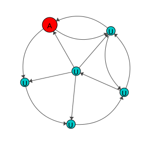
Our experiments are designed to represent stylized enterprise networks where the attacker has penetrated the perimeter and can begin traversing the network. For example, the attacker may have compromised the computer of a credit card customer service representative at a major bank. However, he is not interested in the information available on that machine but is interested in account information held on a central server. As a result, he must emit messages from the originally infected machine in order to gather credentials and elevate privileges until he has access to valuable information. This is however only one possible narrative and the experimental environment can represent any number of enterprise attacks.

In each of our experiments, we generated $400$ realizations of network activity over an observation window length $T$. There are $200$ cases with an attacker and $200$ cases without an attacker. Recall that the dataset available to both of the detectors is a collection of triples of the form $\left(v_{i},v^{\prime}_{i},\tau_{i}\right)$ indicating that a message traversed an edge from $v_{i}$ to $v^{\prime}_{i}$ at time $\tau_{i}$. From such a dataset it is possible to compute the likelihood ratio as well as the baseline likelihood detection criteria, which are both given in section 3. For each realization, we compute the likelihood that the observed message transmissions come from a system with no attacker and the likelihood that the observed message transmissions come from a system with an attacker. The likelihood ratio classifier proposed in the previous section is the ratio of the two likelihoods. The ROC curve for anomaly detection uses only the likelihood of no attacker as the classifier.

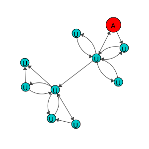
In our first experiment, we analyze a small network as shown in figure 1 for $T=1500$. The “star” formation in figure 1 is a typical subgraph of many computer networks. More generally, the experiments in this section use topologies that are stylized representations of small sections of real-world subgraphs (such as a “star” or a ”caterpillar”). However, these topologies may not be realistic of all real-world networks. To ensure that our results hold for more realistic, larger networks, the “Real Data Experiments” section extracts real-world network topologies from the computer network at Los Alamos National Lab.

Normal message traffic rates are set to $1$ and malicious message transmission was set to $3\%$ of the normal rate, which models a relatively slow attack. Under this scenario, the attacker remains on the network for long periods of time and traverses the network sporadically. %Note that in these initial experiments, we use homogeneous rates of benign message transmission. This allows us to investigate the effects on the ROC curves of changing other model parameters (such as the observation window or rate of malicious message transmission) without having to consider how the effects depend on rate parameter heterogeneity. Nevertheless, the “Real Data Experiments” section considers a high degree of rate heterogeneity and confirm the superiority of the likelihood ratio detector.

Figure 2: ROC curves for the network topology shown in figure 1.

Figure 3: ROC curve under the “enter slowly, traverse quickly” specification.

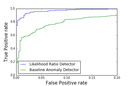
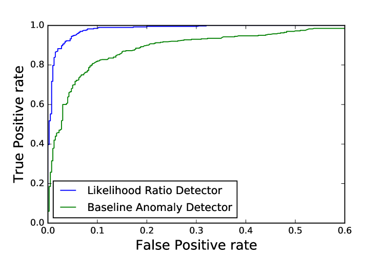
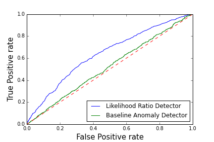
Figure 3 shows that the likelihood ratio detector outperforms the baseline anomaly detector. That is, for any false positive rate the likelihood ratio detector has a higher true positive rate than the simple anomaly detector. Furthermore, figure 3 shows that the superiority of the likelihood ratio detector is clear even for low values of the false positive rate. This is important because in real world networks, limited resources only allow security response teams to investigate a small number of instances and thus must set the threshold to a relatively small rate of false positives. In other words, if the likelihood ratio detector’s superiority was only apparent for relatively high rates of false positives, its benefits would not be realized in practice. However, since the likelihood ratio detector’s advantage is evident for low false positive rates, the initial results suggest that it would improve practical anomaly detection.

Figure 4: ROC with $T=10$.

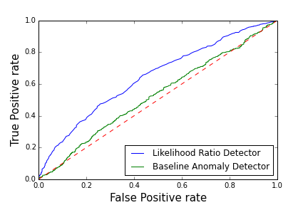
In our second experiment, we consider the same network but adopt an “enter slowly, traverse quickly” strategy for the attacker and use $T=400$. In this scenario, the attacker initially sends messages at a rate of $3\%$ of the initial compromised node’s normal transmission rate. Once inside the network, the attacker traverses the network rapidly by sending messages at a rate of $6\%$ of the normal message rate. Figure 3 once again shows that the likelihood ratio detector dominates the simple anomaly detector. Like figure 3, the dominance of the likelihood ratio detector is evident for low (0) levels of the false positive rate.

Figure 5: Network topology (upper left) and ROC curves for various sets of parameters: Upper right: $T=800$ and all rates 3% normal rates. Lower left: $T=50$ and the rate of malicious messages out of the initially infected node is 3% the normal message rate while malicious messages out of all other nodes is 6% the benign rate. Lower right: $T=10$ and malicious rates are 50% of benign rates except for nodes with more than 2 outgoing edges. For those nodes, the rate of malicious messages is 10% of benign messages.

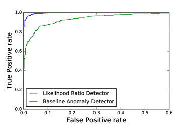
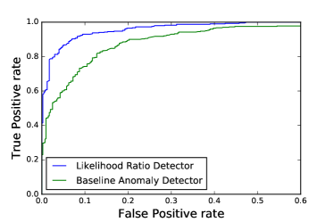
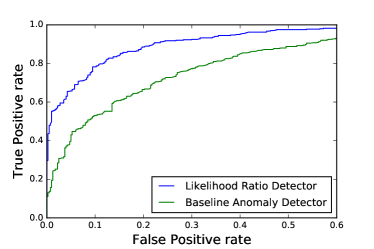
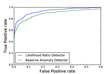
In our third experiment, using the same network and $T=10$, we model an attacker that makes no attempt to “hide” from the detectors, but instead tries to traverse the network fast enough so that by the time an alarm sounds, the network has already been compromised. Malicious message rates are set to half the normal traffic rate. Figure 4 provides the third validation that the likelihood ratio detector performs better than the anomaly detector and indicates that it is possible to detect the attacker before he reaches his goal.

Figure 6: ROC curve under the scenario where the attacker becomes more aggressive as he approaches the goal.

The fourth experiment employs the same three attacker heuristics but this time for the larger network described in figure 5. All benign message transmission rates are once again $1$ and the rate of malicious messages is given in the caption of the figure. The motivativation for this experiment is two-fold. First, it is used to verify that the results of the previous experiments were not specific to a certain network topology. Secondly, the larger network contains more nodes and more edges and thus requires more computational resources to compute the likelihood ratio. Therefore, the larger network serves as a test bed to see if the likelihood ratio detector remains superior under a modest scale increase. The ROC curves indicate that the likelihood ratio detector outperforms the anomaly detector under all three specifications in this case as well.

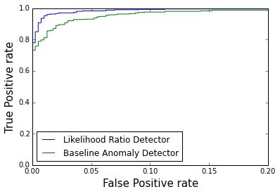
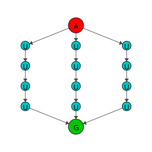
A final test examines the performance of the likelihood ratio detector when the attacker’s strategy is to increase in aggression as he approaches his end target. Figure 8 shows a network where the attacker moves toward a goal (node ’G’). All nodes send normal messages at rate $1$. At node ’A’, the attacker sends malicious messages at rate $.05$. For each subsequent node infection, the malicious message rate increases by $.05$. The observation window is set to $T=12$. Once again, figure 6 shows that the likelihood ratio detector outperforms the simple anomaly detector. This is especially promising since the advantage of the likelihood ratio detector is evident for very low false alarm rates (note the $x$-axis ends at $.2$). Additionally, it shows that the likelihood ratio detector outperforms the simple anomaly detector, even when the simple anomaly detector performs relatively well. (The anomaly detector detects 90% of attacks with a false positive rate of about $.05$ in figure 6 compared to a false positive rate of $.5$ in the top right corner of figure 3). These results along with the previous experiments suggest that the superiority of the likelihood ratio detector exists regardless of the performance of the simple anomaly detector.

Model misspecification

The preceding results assumed that the rate of malicious message transmission and attacker strategy is known. That is, the parameters used to compute the likelihood ratio test statistic were the rates that the attacker actually used. In reality this is not usually the case. Therefore, to test the performance of the likelihood ratio detector in a more realistic scenario we assume that the attacker’s strategy is misspecified and test the performance of the likelihood ratio. In this scenario, we use the network described in Figure 8 with $T=10$ and we set all normal message rates equal to $1$ and compute the likelihood ratio as if the rate of malicious messages is $.5$ on edges exiting any compromised nodes. This model of the attacker allows the detector to hedge for an attacker that could choose any path from $A$ to $G$. In our experiments, the actual attacker only traverses the center path (using rate $.5$). Figure 8 shows that even under misspecification, the likelihood ratio detector is superior to the baseline anomaly detector. In this specific example, the superiority is most pronounced around a false positive rate of $.5$. This is too high to be practically significant but there are also modest performance improvements for low false positive rates. Furthermore, because the likelihood ratio test uses incorrect parameters in the alternative hypothesis, there is not theoretical guarantee that the likelihood ratio outperforms the simple anomaly detector. However, this example shows that for any threshold, the likelihood ratio does at least as well as the simple anomaly detector.

Figure 7: Network topology with misspecified attacker strategy.

Figure 8: ROC curve when the model allows the attacker to take all paths, but he only takes one.

To further test model misspecification, we consider the net in figure 9. This topology is a stylized version of commonly observed attacker behavior as noted in  Neil et al., (2013) In short, an attacker sends messages to all hosts connected to a host he has already compromised. After exploring the hosts connected to the originally compromised host, he will then occupy another host and then begin exploring from that host. This generates what is called a “caterpillar” pattern of malicious behavior.

Figure 9: Network topology and ROC curves for various levels of noise misspecification from upper right to lower right, the standard deviation of the noise is 10, 20 and 30 percent.

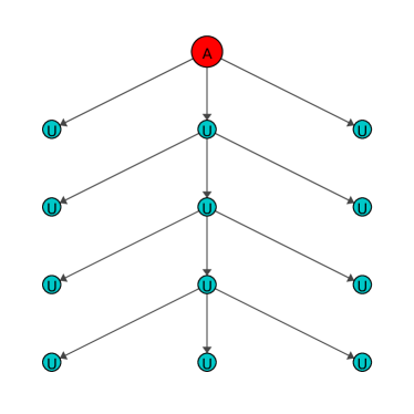
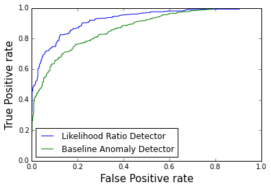
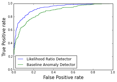
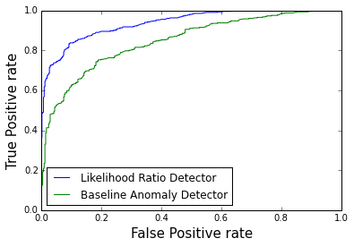
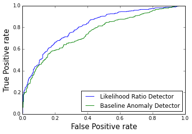
The type of model misspecification analyzed here is one in which the specified rate of attacker behavior is subject to non-systematic error. Since in most cases the attacker is a human with imperfect reasoning, it would be unreasonable to expect to model the attacker’s method exactly. Or on the other hand, it is not likely that an attacker model will be able to perfectly specify what an attacker will do but only be able to determine how attackers will behave on average. To analyze this type of model misspecification, the attacker sends messages along the center path and to the off center hosts in figure 9. (The rate along the center path is $.5$ and off center is $.25$. The rate of background messages is $1$ for all hosts). However, the rate at which the likelihood ratio models the attacker is subject to mean-zero, Gaussian noise with standard deviations of $10$, $20$ and $30$ percent of the actual attacker rate.

Figure 9 shows that even under non-systematic errors in the attacker rates, the likelihood ratio detector still performs better than the simple anomaly detector. Interestingly, increasing the standard deviation of the noise seems to have little to no effect on the performance of the likelihood ratio detector. The slight difference in performance is likely a result of stochasticity of the underlying data generating process.

Figure 10: ROC curve where the attacker is assumed to only take the center path.

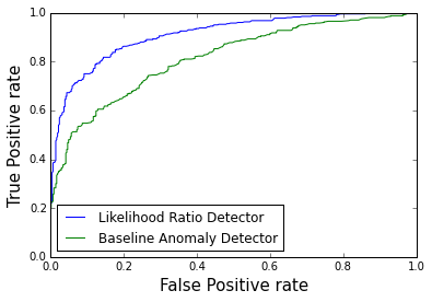
Another test of model misspecification in the caterpillar net is the converse of the misspecification that generated figure 8. For that experiment, we modeled the attacker as traversing any and all possible paths in the network where in reality he only traversed one path. However in this example, we calculate the likelihoods as if the attacker only took the center path of the caterpillar net but in reality, he was actually exploring the left and right hosts.

This type of model misspecification has at least two real world interpretations. The first is that the model misspecifies the attacker as being more intelligent than he actually is. For example, if the attacker’s goal is to traverse the caterpillar to the last center host, he would not gain anything from exploring the nodes off of the center path. However, if the attacker does not know the topology of the network and the location of the valuable information, he will explore the off-center nodes in the network. Therefore, this version of model misspecification models the attacker as more intelligent and efficient than he actually behaves.

Another interpretation is of practical concern. The strength of a likelihood ratio detector will — to some degree — depend on how accurate the model of the attacker is. However, the attacker is a goal driven agent and therefore his behavior would be the result of an optimization problem or even the solution to a fixed point problem. Such problems in complex environments such as a computer network can become intractable with only a small number of hosts (especially fixed point solutions). As a result, it might only be feasible to consider attacker behavior at hosts with the most sensitive information. Therefore, it is imperative for the likelihood ratio detector to be effective, even when it only considers malicious activity along a subset of edges in the network.

Figure  10 shows that the likelihood ratio detector does outperform the simple anomaly detector even when the likelihood ratio assumes the attacker only takes the center path. It is interesting to note that under this specification, the likelihood ratio is being handicapped because the malicious activity off of the center path enters multiplicatively and equally in the numerator and the denominator of the likelihood ratio and therefore cancels. However, the malicious activity off of the center path does provide evidence of an attack when using the simple anomaly detector. In other words, since the likelihood ratio assumes the rate of malicious message transmission off of the center path is $0$, all messages off of the center path are considered as normal background behavior, regardless of how abnormal the messages seem. On the other hand, the simple anomaly detector considers traffic along all edges and therefore abnormal activity off of the center path would push the simple anomaly classification criteria toward the threshold.

4.1 Real Network Experiments

In all of the previous experiments, the network topology and message transmission rates were selected to be a stylized representation of real world networks. To ensure that the results hold for more realistic networks, this section extracts network topologies and estimates message rates from data collected from an active computer network. The data used are the Los Alamos National Lab (LANL) “User-Computer authentication associations in time” (Hagberg et al.,, 2014). The data contain time-stamped user-computer authentication logs. For example, one data point is given by:

U1, C5, 1

which represents a user with an anonymous identification number $U1$ logging into a host with identification number $C5$ at time $1$. The data are taken over a period of nine months and the unit of time is seconds. The time stamps are given in whole numbers and therefore the data are binned into seconds.

Concurrent connection attempts by the same user constitute communication between two hosts.Suppose, for example, $U1$ logs into $C1$ and then in the same second $U1$ logs into $C2$, then a communication is inferred, which is then modeled as a directed edge from $C1$ and $C2$. The network topology is constructed in this way because of the following logging artifact: If $U1$ is logged onto $C1$ and successfully logs onto $C2$, the authentication log will record $2$ entries. The first will be an authentication log at $C1$; user $1$ must be authenticated at $C1$ in order to log onto other hosts. The second will be a recording at $C2$ that notes a successful authentication into $C2$. In the language of the preceding section, an authentication attempt is a “message.”

Since the dataset covers nine months of authentication requests, which includes $11,362$ users and $22,284$ computers, the computational approach only allows for the analysis of a subset of the network at a relatively small slice in time. To do this, only one hour intervals in the first month of the dataset are considered. However, due to computational limitations only the elements of the network that see the most traffic are included. This modeling choice is motivated by two generally observed patterns. First, the part of the network with the most traffic is where it will be most difficult to detect an attacker. In other words, an attacker’s rate is always relatively low. Therefore, if the background rate between hosts is relatively high, the attacker’s signal to noise ratio is low, thus rendering detection more difficult. On the other hand, it is easier for an attacker to go undetected when there are many users logging into a specific machine. The second motivation is that high traffic areas are likely to be the location of valuable information and hence be a likely location to deploy a novel attack detector. The reason for this is that central servers typically contain the most valuable information and therefore often receive the most traffic.

To extract a subgraph for analysis, a random hour in the first month of the data is sampled and then a full graph is created based on the method described above. From the full graph, any nodes (and corresponding edges into and out of the node) that do not have more than $15$ incoming messages and $15$ outgoing messages are removed. This results in several disconnected subgraphs. The final graph is the largest connected component. The estimate of the per hour message transmission rate is simply the one hour message count. That rate is used to simulate the background messages. That is, actual message times are not used as the observed data. Instead, the observed messages are used to estimate a Poisson rate to generate the times of normal message transmission. The distribution of per minute message rates between nodes in the two extracted topologies is given in figure 11. The figure indicates that there is significant rate heterogeneity with the highest rate being more than $10$ times that of the lowest rate in each experiment.

Figure 11: The distribution of Poisson rates extracted from the LANL network.

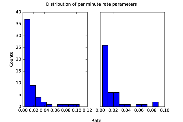
Although using the actual message times would be a more accurate representation of the real data, time heterogeneity of the rate constants would significantly increase both the model sophistication as well as the computational requirement to carry out the likelihood calculation in this initial framework. In other words, although in a small time window, message transmission counts can be described by a Poisson or negative binomial distribution, this rate changes throughout the working day (and the weekend). Therefore, the likelihood ratio in section 3 would have to incorporate a stochastic process that defines the behavior of the background message transmission rates, thus adding another dimension to the integral calculation in the denominator of the likelihood. Such modeling remains a topic of future work. Furthermore, since the ROC analysis of the real data requires $800$ simulations of the network, there are not enough data points to carry out an accurate ROC analysis. In other words, even if it was known that on Tuesdays from 12PM to 1PM, the rate of message transmission was always the same, the data only contains 36 such occasions which is not sufficient for ROC analysis.

Since the dataset does not contain attack data, the rate of malicious messages transmission is set to 10% of the background rate. Since it is also not known which node might be initially compromised, multiple experiments are performed in which the initially compromised node is uniformly sampled.

Real Data Results and Discussion

The first subgraph analyzed is depicted in figure 12. The numbered nodes correspond to the attacker’s starting point for each of the experiments. The ROC curves that compare the likelihood ratio detector to the simple anomaly detector are given in figure 13. The second subgraph analyzed is depicted in figure  14 and the associated ROC curves are in figure 13. In all of the results, the network is simulated for $T=60$ minutes.

Figure 12: First network topology extracted from LANL network.

Figure 13: ROC results for real network topologies. The plots from left to right represent attacker starting points 1-5 as numbered in figure  12.

Figure 14: Second network topology extracted from LANL network.

Figure 15: ROC results for real network topologies. The plots from left to right represent attacker starting points 1-5 as numbered in figure  14.

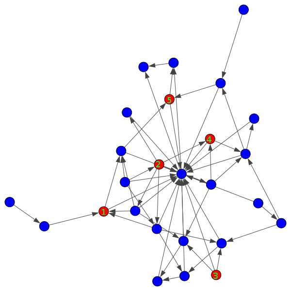
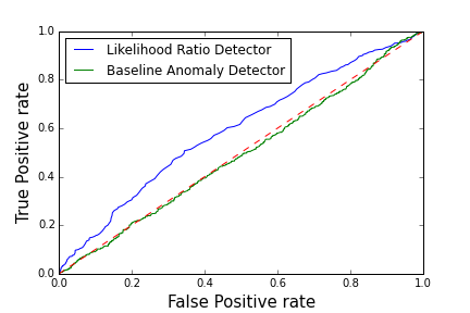
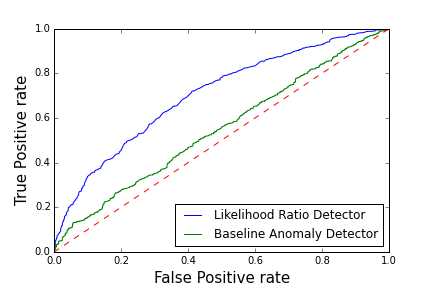
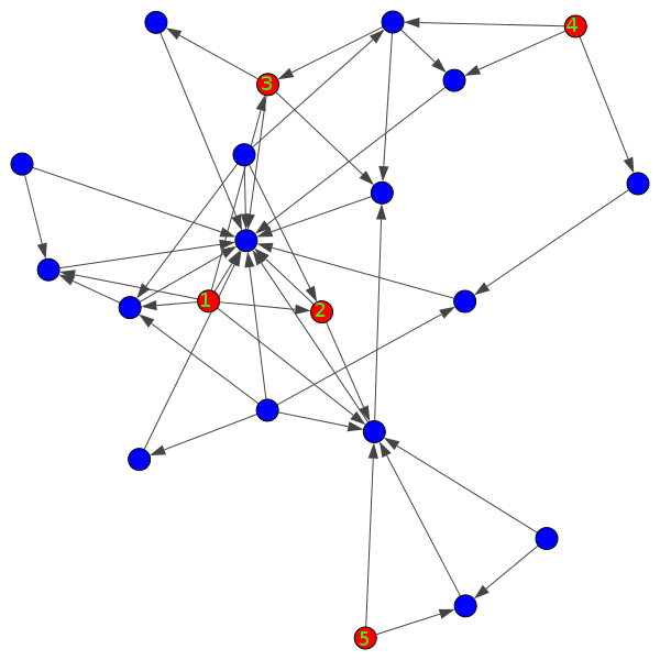
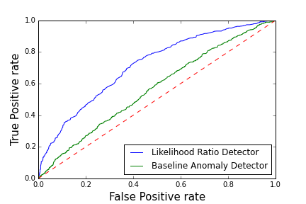
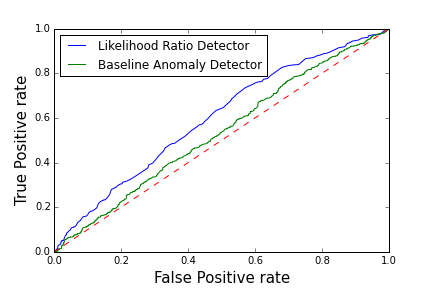
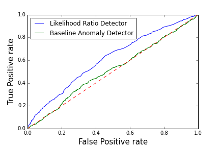
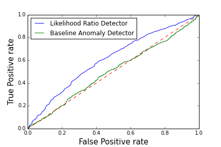
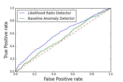
From the figures, it is clear that the likelihood ratio detector is superior at all threshold levels to the simple anomaly detector. Interestingly, the overall performance of both detectors seem to perform worse in the real network than in the simulated network. The reason for this is that in the real network, only a subset of the nodes can become compromised. For example, in figure  14 where the attacker initially has compromised node numbered 2, only three of the 21 nodes can possibly become compromised. Therefore, the signal of the attacker behavior is low compared to the background noise generated by the entire network. In the previous experiments, it was possible for a greater proportion of nodes to become compromised. Nevertheless, the likelihood ratio detector still outperforms the simple anomaly detector in all scenarios.

It is also interesting to note that even when the simple anomaly detector performs no better than random guessing (in the figures, this is the case when the line representing the simple anomaly detector is almost the same as the dashed line which represents the performance of uniform random guessing), the likelihood ratio detector offers a slight advantage over random guessing. The reason for this is due to the definition of a likelihood. More specifically, the likelihood can be relatively low due to the presence of an attacker. However, the likelihood can also be low due to an atypical lack of activity. In this case, the low signal to noise ratio coupled with the simple anomaly detector sometimes classifies low traffic as anomalous causes the detector to perform no better than random. Note that anomalous low traffic — a phenomenon almost certainly not indicative of an attacker — does not affect the likelihood ratio’s classification performance as this type of behavior will appear in both the numerator and denominator and cancel. This can be solved in the anomaly detector by restricting the parameter space to test for rate increases, as is done in Neil et al., (2013). However, the attacker model proposed incorporates more information than just rate increase testing, and therefore performs better.

Summary of Results
Graph Topology	ROC Curve	Misspecified Rates?(Y/N)	Clear Dominance at False Positive Rate $<.05$? (Y/N)	Likelihood Ratio No worse at all False Positive Rates?
1	Fig. 3, 3 4	N	Y	Y
Fig. 5 (Top Left)	Fig. 5 (Top Right, Bottom Right)	N	Y	Y
Fig. 5 (Top Left)	Fig. 5 (Bottom Left)	N	N	Y
Fig. 8	Fig 6	N	Y	Y
Fig. 8	Fig. 8	Y	N	Y
Fig. 9 (Top Right)	Fig. 9 (All)	Y	Y	Y
Fig. 9 (Top Right)	Fig. 10	Y	Y	Y
Fig. 12	Fig. 13 (All)	N	Y	Y
Fig. 14	Fig. 15 (All)	N	Y	Y

Table 1: Results of ROC experiments: The first column gives the figure representing the graph topology. The second column gives the ROC curve for the experiment. The third column notes if the likelihood ratio detector is clearly superior at a false positive rate of .05 and less. The final column notes whether the likelihood ratio detector performs at least as good as the simple anomaly detector for all false positive rates and better at one or more false positive rates.

Table 1 provides a brief summary of all experiments.

5 Future work

There are many ways that our model of the behavior of a network can be extended. Most straightforwardly, by incorporating a loss function for incorrect alerts and specifying a prior probability of there being an attacker, we should be able to construct a Bayesian decision-theoretic extension of our anomaly detector.

Other future work involves applying our modeling approach for more realistic networks. This will likely require us to consider other approaches to evaluating our likelihood, e.g., importance sampling or MCMC, rather than simple sampling. Indeed, it may even be possible to do closed form evaluation of our integrals, using the Laplace convolution theorem (Wolpert and DeDeo,, 2013).

It should be possible to use our model to make predictions for any scenario in which humans interact with technical systems in continuous time, and our observational data is limited. In other future work we will apply our models to make predictions in such scenarios. (See also Wolpert and Bono, (2015).) This should allow us to address any statistical question concerning such scenarios, not just for anomaly detection.

Finally, we have started to extend our approach to model not just a single human interacting with a technology system, but a set of humans, interacting with one another as well as that underlying technology system (Wolpert et al.,, 2013). This extension can be viewed as an “event-driven” non-cooperative game theoretic approach, which is distinct from both differential games (in which player moves are real-valued, and chosen continually, at all times) and Markov games (which lack hidden variables). Future work involves investigating this event-driven game theory and its application to likelihood ratio based attack detection.

6 Acknowledgments

The authors would like to acknowledge the Army Research Office (ARO) for supporting this work under grant number W911NF15-1-0127.

References

- Borgwardt et al., (2006) Borgwardt, K. M., Kriegel, H.-P., and Wackersreuther, P. (2006). Pattern mining in frequent dynamic subgraphs. In Data Mining, 2006. ICDM’06. Sixth International Conference on, pages 818–822. IEEE.
- Chandola et al., (2009) Chandola, V., Banerjee, A., and Kumar, V. (2009). Anomaly detection: A survey. ACM Computing Surveys (CSUR), 41(3):15.
- Djidjev et al., (2011) Djidjev, H., Sandine, G., Storlie, C., and Vander Wiel, S. (2011). Graph based statistical analysis of network traffic. In Proceedings of the Ninth Workshop on Mining and Learning with Graphs.
- Eberle et al., (2010) Eberle, W., Graves, J., and Holder, L. (2010). Insider threat detection using a graph-based approach. Journal of Applied Security Research, 6(1):32–81.
- Garcia-Teodoro et al., (2009) Garcia-Teodoro, P., Diaz-Verdejo, J., Maciá-Fernández, G., and Vázquez, E. (2009). Anomaly-based network intrusion detection: Techniques, systems and challenges. computers & security, 28(1):18–28.
- Gillespie, (1977) Gillespie, D. T. (1977). Exact stochastic simulation of coupled chemical reactions. The journal of physical chemistry, 81(25):2340–2361.
- Hagberg et al., (2014) Hagberg, A., Kent, A., Lemons, N., and Neil, J. (2014). Credential hopping in authentication graphs. In 2014 International Conference on Signal-Image Technology Internet-Based Systems (SITIS). IEEE Computer Society.
- Jiang et al., (2011) Jiang, D., Xu, Z., Chen, Z., Han, Y., and Xu, H. (2011). Joint time–frequency sparse estimation of large-scale network traffic. Computer Networks, 55(15):3533 – 3547.
- (9) Jiang, D., Xu, Z., and Xu, H. (2015a). A novel hybrid prediction algorithm to network traffic. annals of telecommunications - annales des télécommunications, 70(9-10):427–439.
- (10) Jiang, D., Xu, Z., Zhang, P., and Zhu, T. (2014a). A transform domain-based anomaly detection approach to network-wide traffic. Journal of Network and Computer Applications, 40:292 – 306.
- (11) Jiang, D., Yao, C., Xu, Z., and Qin, W. (2015b). Multi-scale anomaly detection for high-speed network traffic. Transactions on Emerging Telecommunications Technologies, 26(3):308–317.
- (12) Jiang, D., Zhao, Z., Xu, Z., Yao, C., and Xu, H. (2014b). How to reconstruct end-to-end traffic based on time-frequency analysis and artificial neural network. {AEU} - International Journal of Electronics and Communications, 68(10):915 – 925.
- Kang et al., (2009) Kang, J., Zhang, J.-Y., Li, Q., and Li, Z. (2009). Detecting new p2p botnet with multi-chart cusum. In Networks Security, Wireless Communications and Trusted Computing, 2009. NSWCTC ’09. International Conference on, volume 1, pages 688–691.
- Kantas et al., (2009) Kantas, N., Doucet, A., Singh, S. S., and Maciejowski, J. M. (2009). Overview of sequential monte carlo methods for parameter estimation on general state space models. In Proc. 15th IFAC Symposium on System Identification (SYSID) 2009, Saint-Malo, France.
- Kent and Liebrock, (2013) Kent, A. D. and Liebrock, L. M. (2013). Differentiating user authentication graphs. In Security and Privacy Workshops (SPW), 2013 IEEE, pages 72–75. IEEE.
- Krebs, (2014) Krebs, B. (2014). The target breach, by the numbers. http://krebsonsecurity.com/2014/05/the-target-breach-by-the-numbers/.
- Krebs, (2015) Krebs, B. (2015). Data breach at health insurer anthem could impact millions. http://krebsonsecurity.com/2015/02/data-breach-at-health-insurer-anthem-could-impact-millions/.
- Kumaraguru et al., (2009) Kumaraguru, P., Cranshaw, J., Acquisti, A., Cranor, L., Hong, J., Blair, M. A., and Pham, T. (2009). School of phish: a real-world evaluation of anti-phishing training. In Proceedings of the 5th Symposium on Usable Privacy and Security, page 3. ACM.
- Lee and Stolfo, (2000) Lee, W. and Stolfo, S. J. (2000). Data mining approaches for intrusion detection. Defense Technical Information Center.
- Lee and Xiang, (2001) Lee, W. and Xiang, D. (2001). Information-theoretic measures for anomaly detection. In Security and Privacy, 2001. S&P 2001. Proceedings. 2001 IEEE Symposium on, pages 130–143. IEEE.
- Neil et al., (2013) Neil, J., Hash, C., Brugh, A., Fisk, M., and Storlie, C. B. (2013). Scan statistics for the online detection of locally anomalous subgraphs. Technometrics, 55(4):403–414.
- Robert and Casella, (2004) Robert, C. P. and Casella, G. (2004). Monte Carlo Statistical Methods. Springer-Verlag, New York.
- Roesch et al., (1999) Roesch, M. et al. (1999). Snort: Lightweight intrusion detection for networks. In LISA, volume 99, pages 229–238.
- Ryan et al., (1998) Ryan, J., Lin, M.-J., and Miikkulainen, R. (1998). Intrusion detection with neural networks. In Advances in neural information processing systems, pages 943–949. MORGAN KAUFMANN PUBLISHERS.
- Sommer and Paxson, (2010) Sommer, R. and Paxson, V. (2010). Outside the closed world: On using machine learning for network intrusion detection. In Security and Privacy (SP), 2010 IEEE Symposium on, pages 305–316. IEEE.
- Staniford-Chen et al., (1996) Staniford-Chen, S., Cheung, S., Crawford, R., Dilger, M., Frank, J., Hoagland, J., Levitt, K., Wee, C., Yip, R., and Zerkle, D. (1996). Grids-a graph based intrusion detection system for large networks. In Proceedings of the 19th national information systems security conference, volume 1, pages 361–370. Baltimore.
- Thatte et al., (2008) Thatte, G., Mitra, U., and Heidemann, J. (2008). Detection of low-rate attacks in computer networks. In INFOCOM Workshops 2008, IEEE, pages 1–6. IEEE.
- Wang et al., (2004) Wang, H., Zhang, D., and Shin, K. (2004). Change-point monitoring for the detection of dos attacks. Dependable and Secure Computing, IEEE Transactions on, 1(4):193–208.
- Wolpert and Bono, (2015) Wolpert, D. and Bono, J. (2015). Distribution-valued solution concepts. Review of Behavioral Economics. in press.
- Wolpert et al., (2013) Wolpert, D. H., Bhattacharya, T., Bent, R., Neil, J., Kent, A., and Giani, A. (2013). Event-driven non-cooperative games, la-ur-13-22238. Technical report, Los Alamos National Laboratory.
- Wolpert and DeDeo, (2013) Wolpert, D. H. and DeDeo, S. (2013). Estimating functions of distributions defined over spaces of unknown size. Entropy, 15(11):4668–4699.