All Fingers are not Equal: Intensity of References in Scientific Articles
(Accepted in EMNLP, 2016)

Abstract

Research accomplishment is usually measured by considering all citations with equal importance, thus ignoring the wide variety of purposes an article is being cited for. Here, we posit that measuring the intensity of a reference is crucial not only to perceive better understanding of research endeavor, but also to improve the quality of citation-based applications. To this end, we collect a rich annotated dataset with references labeled by the intensity, and propose a novel graph-based semi-supervised model, GraLap  to label the intensity of references. Experiments with AAN datasets show a significant improvement compared to the baselines to achieve the true labels of the references (46% better correlation). Finally, we provide four applications to demonstrate how the knowledge of reference intensity leads to design better real-world applications.

1 Introduction

With more than one hundred thousand new scholarly articles being published each year, there is a rapid growth in the number of citations for the relevant scientific articles. In this context, we highlight the following interesting facts about the process of citing scientific articles: (i) the most commonly cited paper by Gerard Salton, titled “A Vector Space Model for Information Retrieval” (alleged to have been published in 1975) does not actually exist in reality [Dubin, 2004], (ii) the scientific authors read only 20% of the works they cite [Simkin and Roychowdhury, 2003], (iii) one third of the references in a paper are redundant and 40% are perfunctory [Moravcsik and Murugesan, 1975], (iv) 62.7% of the references could not be attributed a specific function (definition, tool etc.) [Teufel et al., 2006]. Despite these facts, the existing bibliographic metrics consider that all citations are equally significant.

In this paper, we would emphasize the fact that all the references of a paper are not equally influential. For instance, we believe that for our current paper, [Wan and Liu, 2014] is more influential reference than [Garfield, 2006], although the former has received lower citations (9) than the latter (1650) so far. Therefore the influence of a cited paper completely depends upon the context of the citing paper, not the overall citation count of the cited paper. We further took the opinion of the original authors of few selective papers and realized that around 16% of the references in a paper are highly influential, and the rest are trivial (Section 4). This motivates us to design a prediction model, GraLap  to automatically label the influence of a cited paper with respect to a citing paper. Here, we label paper-reference pairs rather than references alone, because a reference that is influential for one citing paper may not be influential with equal extent for another citing paper.

We experiment with ACL Anthology Network (AAN) dataset and show that GraLap  along with the novel feature set, quite efficiently, predicts the intensity of references of papers, which achieves (Pearson) correlation of $0.90$ with the human annotations. Finally, we present four interesting applications to show the efficacy of considering unequal intensity of references, compared to the uniform intensity.

The contributions of the paper are four-fold: (i) we acquire a rich annotated dataset where paper-reference pairs are labeled based on the influence scores (Section 4), which is perhaps the first gold-standard for this kind of task; (ii) we propose a graph-based label propagation model GraLap for semi-supervised learning which has tremendous potential for any task where the training set is less in number and labels are non-uniformly distributed (Section 3); (iii) we propose a diverse set of features (Section 3.3); most of them turn out to be quite effective to fit into the prediction model and yield improved results (Section 5); (iv) we present four applications to show how incorporating the reference intensity enhances the performance of several state-of-the-art systems (Section 6).

2 Defining Intensity of References

All the references of a paper usually do not carry equal intensity/strength with respect to the citing paper because some papers have influenced the research more than others. To pin down this intuition, here we discretize the reference intensity by numerical values within the range of $1$ to $5$, ($5$: most influential, $1$: least influential). The appropriate definitions of different labels of reference intensity are presented in Figure 1, which are also the basis of building the annotated dataset (see Section 4):

Figure 1: Definitions of the intensity of references

$\bullet$ Label-1: The reference is related to the citing article with very limited extent and can be removed without compromising the competence of the references (e.g., [Garfield, 2006] for this paper).
$\bullet$ Label-2: The reference is little mentioned in the citing article and can be replaced by others without compromising the adequacy of the references (e.g., [Zhu et al., 2015] for this paper).
$\bullet$ Label-3: The reference occurs separately in a sentence within the citing article and has no significant impact on the current problem (e.g., references to metrics, tools) (e.g., [Porter, 1997] for this paper).
$\bullet$ Label-4: The reference is important and highly related to the citing article. It is usually mentioned several times in the article with long reference context (e.g., [Singh et al., 2015] for this paper).
$\bullet$ Label-5: The reference is extremely important and occurs (is emphasized) multiple times within the citing article. It generally points to the cited article from where the citing article borrows main ideas (and can be treated as a baseline) (e.g., [Wan and Liu, 2014] for this paper).

Note that “reference intensity” and “reference similarity” are two different aspects. It might happen that two similar reference are used with different intensity levels in a citing paper – while one is just mentioned somewhere in the paper and other is used as a baseline. Here, we address the former problem as a semi-supervised learning problem with clues taken from content of the citing and cited papers.

3 Reference Intensity Prediction Model

In this section, we formally define the problem and introduce our prediction model.

3.1 Problem Definition

We are given a set of papers $\mathbb{P}=\{P_{1},P_{2},...,P_{M}\}$ and a sets of references $\mathbb{R}=\{R_{1},R_{2},...,R_{M}\}$, where $R_{i}$ corresponds to the set of references (or cited papers) of $P_{i}$. There is a set of papers $P_{L}\in\mathbb{P}$ whose references $R_{L}\in\mathbb{R}$ are already labeled by $\ell\in L=\{1,...,5\}$ (each reference is labeled with exactly one value). Our objective is to define a predictive function $f$ that labels the references $R_{U}\in\{\mathbb{R}\setminus R_{L}\}$ of the papers $P_{U}\in\{\mathbb{P}\setminus P_{L}\}$ whose reference intensities are unknown, i.e., $f:(\mathbb{P},\mathbb{R},P_{L},R_{L},P_{U},R_{L})\longrightarrow L$.

Since the size of the annotated (labeled) data is much smaller than unlabeled data ($|P_{L}|\ll|P_{U}|$), we consider it as a semi-supervised learning problem.

Definition 1.

(Semi-supervised Learning) Given a set of entries $X$ and a set of possible labels $Y_{L}$, let us assume that ($x_{1},y_{1}$), ($x_{2},y_{2}$),…, ($x_{l},y_{l}$) be the set of labeled data where $x_{i}$ is a data point and $y_{i}\in Y_{L}$ is its corresponding label. We assume that at least one instance of each class label is present in the labeled dataset. Let ($x_{l+1},y_{l+1}$), ($x_{l+2},y_{l+2}$),…, ($x_{l+n},y_{l+u}$) be the unlabeled data points where $Y_{U}={\{y_{l+1},y_{l+2},...y_{l+u}\}}$ are unknown. Each entry $x\in X$ is represented by a set of features $\{f_{1},f_{2},...,f_{D}\}$. The problem is to determine the unknown labels using $X$ and $Y_{L}$.

3.2 GraLap: A Prediction Model

We propose GraLap, a variant of label propagation (LP) model proposed by [Zhu et al., 2003] where a node in the graph propagates its associated label to its neighbors based on the proximity. We intend to assign same label to the vertices which are closely connected. However unlike the traditional LP model where the original values of the labels continue to fade as the algorithm progresses, we systematically handle this problem in GraLap. Additionally, we follow a post-processing in order to handle “class-imbalance problem”.
Graph Creation. The algorithm starts with the creation of a fully connected weighted graph $G=(X,E)$ where nodes are data points and the weight $w_{ij}$ of each edge $e_{ij}\in E$ is determined by the radial basis function as follows:

$$\small w_{ij}=exp\bigg{(}-\frac{\sum_{d=1}^{D}(x_{i}^{d}-x_{j}^{d})^{2}}{\sigma^{2}}\bigg{)}$$ (1)

The weight is controlled by a parameter $\sigma$. Later in this section, we shall discuss how $\sigma$ is selected. Each node is allowed to propagate its label to its neighbors through edges (the more the edge weight, the easy to propagate).
Transition Matrix. We create a probabilistic transition matrix $T_{|X|\times|X|}$, where each entry $T_{ij}$ indicates the probability of jumping from $j$ to $i$ based on the following: $T_{ij}=P(j\rightarrow i)=\frac{w_{ij}}{\sum_{k=1}^{|X|}w_{kj}}$.
Label Matrix. Here, we allow a soft label (interpreted as a distribution of labels) to be associated with each node. We then define a label matrix $Y_{|X|\times|L|}$, where $i$th row indicates the label distribution for node $x_{i}$. Initially, $Y$ contains only the values of the labeled data; others are zero.
Label Propagation Algorithm. This algorithm works as follows:

1:Initialize $T$ and $Y$ 2:while ($Y$ does not converge) do 3:    $Y\leftarrow TY$ 4:    Normalize rows of $Y$, $y_{ij}=\frac{y_{ij}}{\sum_{k}y_{ik}}$ 5:    Reassign original labels to $X_{L}$

After initializing $Y$ and $T$, the algorithm starts by disseminating the label from one node to its neighbors (including self-loop) in one step (Step 3). Then we normalize each entry of $Y$ by the sum of its corresponding row in order to maintain the interpretation of label probability (Step 4). Step 5 is crucial; here we want the labeled sources $X_{L}$ to be persistent. During the iterations, the initial labeled nodes $X_{L}$ may fade away with other labels. Therefore we forcefully restore their actual label by setting $y_{il}=1$ (if $x_{i}\in X_{L}$ is originally labeled as $l$), and other entries ($\forall_{j\neq l}y_{ij}$) by zero. We keep on “pushing” the labels from the labeled data points which in turn pushes the class boundary through high density data points and settles in low density space. In this way, our approach intelligently uses the unlabeled data in the intermediate steps of the learning.
Assigning Final Labels. Once $Y_{U}$ is computed, one may take the most likely label from the label distribution for each unlabeled data. However, this approach does not guarantee the label proportion observed in the annotated data (which in this case is not well-separated as shown in Section 4). Therefore, we adopt a label-based normalization technique. Assume that the label proportions in the labeled data are $c_{1},...,c_{|L|}$ (s.t. $\sum_{i=1}^{|L|}c_{i}=1)$. In case of $Y_{U}$, we try to balance the label proportion observed in the ground-truth. The label mass is the column sum of $Y_{U}$, denoted by $Y_{U_{.1}},...,Y_{U_{.|L|}}$, each of which is scaled in such a way that $Y_{U_{.1}}:...:Y_{U_{.|L|}}=c_{1}:...:c_{|L|}$. The label of an unlabeled data point is finalized as the label with maximum value in the row of $Y$.
Convergence. Here we briefly show that our algorithm is guaranteed to converge. Let us combine Steps 3 and 4 as $Y\leftarrow\hat{T}Y$, where $\hat{T}=T_{ij}/{\sum_{k}T_{ik}}$. $Y$ is composed of $Y_{L_{l\times|L|}}$ and $Y_{U_{u\times|L|}}$, where $Y_{U}$ never changes because of the reassignment. We can split $\hat{T}$ at the boundary of labeled and unlabeled data as follows:

$$\scriptsize\hat{F} =\begin{bmatrix}\hat{T}_{ll}&\hat{T}_{lu}\\ \hat{T}_{ul}&\hat{T}_{uu}\end{bmatrix}$$

Therefore, $Y_{U}\leftarrow\hat{T}_{uu}Y_{U}+\hat{T}_{ul}Y_{L}$, which can lead to $Y_{U}=\lim_{n\to\infty}\hat{T}_{uu}^{n}Y^{0}+[\sum_{i=1}^{n}\hat{T}_{uu}^{(i-1)}]\hat{T}_{ul}Y_{L}$, where $Y^{0}$ is the shape of $Y$ at iteration $0$. We need to show $\hat{T}_{uu_{ij}}^{n}Y^{0}\leftarrow 0$. By construction, $\hat{T}_{ij}\geq 0$, and since $\hat{T}$ is row-normalized, and $\hat{T}_{uu}$ is a part of $\hat{T}$, it leads to the following condition: $\exists\gamma<1,\ \sum_{j=1}^{u}\hat{T}_{uu_{ij}}\leq\gamma,~{}\forall i=1,...,u$. So,

$$\scriptsize\begin{split}\sum_{j}\hat{T}_{uu_{ij}}^{n}&=\sum_{j}\sum_{k}\hat{T}_{uu_{ik}}^{(n-1)}\hat{T}_{uu_{kj}}\\ &=\sum_{k}\hat{T}_{uu_{ik}}^{(n-1)}\sum_{j}\hat{T}_{uu_{ik}}\\ &\leq\sum_{k}\hat{T}_{uu_{ik}}^{(n-1)}\gamma\\ &\leq\gamma^{n}\end{split}$$

Therefore, the sum of each row in $\hat{T}_{uu_{ij}}^{n}$ converges to zero, which indicates $\hat{T}_{uu_{ij}}^{n}Y^{0}\leftarrow 0$.
Selection of $\sigma$. Assuming a spatial representation of data points, we construct a minimum spanning tree using Kruskal’s algorithm [Kruskal, 1956] with distance between two nodes measured by Euclidean distance. Initially, no nodes are connected. We keep on adding edges in increasing order of distance. We choose the distance (say, $d_{f}$) of the first edge which connects two components with different labeled points in them. We consider $d_{f}$ as a heuristic to the minimum distance between two classes, and arbitrarily set $\sigma=d_{0}/3$, following $3\sigma$ rule of normal distribution [Pukelsheim, 1994].

Table 1: Manually curated lists of words collected from analyzing the reference contexts. The lists are further expanded using the Wordnet:Synonym with different lexical variations. Note that while searching the occurrence of these words in reference contexts, we use different lexical variations of the words instead of exact matching.

Rel	pivotal, comparable, innovative, relevant, relevantly, inspiring, related, relatedly, similar, similarly, applicable, appropriate,
	pertinent, influential, influenced, original, originally, useful, suggested, interesting, inspired, likewise
	recent, recently, latest, later, late, latest, up-to-date, continuing, continued, upcoming, expected, update, renewed, extended
Rec	subsequent, subsequently, initial, initially, sudden, current, currently, future, unexpected, previous, previously, old,
	ongoing, imminent, anticipated, unprecedented, proposed, startling, preliminary, ensuing, repeated, reported, new, earlier,
	earliest, early, existing, further, revised, improved
Ext	greatly, awfully, drastically, intensely, acutely, almighty, exceptionally, excessively, exceedingly, tremendously, importantly
	significantly, notably, outstandingly
Comp	easy, easier, easiest, vague, vaguer, vaguest, weak, weaker, weakest, strong, stronger, strongest, bogus, unclear

3.3 Features for Learning Model

We use a wide range of features that suitably represent a paper-reference pair ($P_{i},R_{ij}$), indicating $P_{i}$ refers to $P_{j}$ through reference $R_{ij}$. These features can be grouped into six general classes.

3.3.1 Context-based Features (CF)

The “reference context” of $R_{ij}$ in $P_{i}$ is defined by three-sentence window (sentence where $R_{ij}$ occurs and its immediate previous and next sentences). For multiple occurrences, we calculate its average score. We refer to “reference sentence” to indicate the sentence where $R_{ij}$ appears.
(i) CF:Alone. It indicates whether $R_{ij}$ is mentioned alone in the reference context or together with other references.
(ii) CF:First. When $R_{ij}$ is grouped with others, this feature indicates whether it is mentioned first (e.g., “[2]” is first in “[2,4,6]”).

Next four features are based on the occurrence of words in the corresponding lists created manually (see Table 1) to understand different aspects.
(iii) CF:Relevant. It indicates whether $R_{ij}$ is explicitly mentioned as relevant in the reference context (Rel in Table 1).
(iv) CF:Recent. It tells whether the reference context indicates that $R_{ij}$ is new (Rec in Table 1).
(v) CF:Extreme. It implies that $R_{ij}$ is extreme in some way (Ext in Table 1).
(vi) CF:Comp. It indicates whether the reference context makes some kind of comparison with $R_{ij}$ (Comp in Table 1).

Note we do not consider any sentiment-based features as suggested by [Zhu et al., 2015].

3.3.2 Similarity-based Features (SF)

It is natural that the high degree of semantic similarity between the contents of $P_{i}$ and $P_{j}$ indicates the influence of $P_{j}$ in $P_{i}$. We assume that although the full text of $P_{i}$ is given, we do not have access to the full text of $P_{j}$ (may be due to the subscription charge or the unavailability of the older papers). Therefore, we consider only the title of $P_{j}$ as a proxy of its full text. Then we calculate the cosine-similarity between the title (T) of $P_{j}$ and (i) SF:TTitle. the title, (ii) SF:TAbs. the abstract, SF:TIntro. the introduction, (iv) SF:TConcl. the conclusion, and (v) SF:TRest. the rest of the sections (sections other than abstract, introduction and conclusion) of $P_{i}$.

We further assume that the “reference context” (RC) of $P_{j}$ in $P_{i}$ might provide an alternate way of summarizing the usage of the reference. Therefore, we take the same similarity based approach mentioned above, but replace the title of $P_{j}$ with its RC and obtain five more features: (vi) SF:RCTitle, (vii) SF:RCAbs, (viii) SF:RCIntro, (ix) SF:RCConcl and (x) SF:RCRest. If a reference appears multiple times in a citing paper, we consider the aggregation of all $RC$s together.

3.3.3 Frequency-based Feature (FF)

The underlying assumption of these features is that a reference which occurs more frequently in a citing paper is more influential than a single occurrence [Singh et al., 2015]. We count the frequency of $R_{ij}$ in (i) FF:Whole. the entire content, (ii) FF:Intro. the introduction, (iii) FF:Rel. the related work, (iv) FF:Rest. the rest of the sections (as mentioned in Section 3.3.2) of $P_{i}$. We also introduce (v) FF:Sec. to measure the fraction of different sections of $P_{i}$ where $R_{ij}$ occurs (assuming that appearance of $R_{ij}$ in different sections is more influential). These features are further normalized using the number of sentences in $P_{i}$ in order to avoid unnecessary bias on the size of the paper.

3.3.4 Position-based Features (PF)

Position of a reference in a paper might be a predictive clue to measure the influence [Zhu et al., 2015]. Intuitively, the earlier the reference appears in the paper, the more important it seems to us. For the first two features, we divide the entire paper into two parts equally based on the sentence count and then see whether $R_{ij}$ appears (i) PF:Begin. in the beginning or (ii) PF:End. in the end of $P_{i}$. Importantly, if $R_{ij}$ appears multiple times in $P_{i}$, we consider the fraction of times it occurs in each part.

For the other two features, we take the entire paper, consider sentences as atomic units, and measure position of the sentences where $R_{ij}$ appears, including (iii) PF:Mean. mean position of appearance, (iv) PF:Std. standard deviation of different appearances. These features are normalized by the total length (number of sentences) of $P_{i}$. , thus ranging from $0$ (indicating beginning of $P_{i}$) to $1$ (indicating the end of $P_{i}$).

3.3.5 Linguistic Features (LF)

The linguistic evidences around the context of $R_{ij}$ sometimes provide clues to understand the intrinsic influence of $P_{j}$ on $P_{i}$. Here we consider word level and structural features.
(i) LF:NGram. Different levels of $n$-grams ($1$-grams, $2$-grams and $3$-grams) are extracted from the reference context to see the effect of different word combination [Athar and Teufel, 2012].
(ii) LF:POS. Part-of-speech (POS) tags of the words in the reference sentence are used as features [Jochim and Schütze, 2012].
(iii) LF:Tense. The main verb of the reference sentence is used as a feature [Teufel et al., 2006].
(iv) LF:Modal. The presence of modal verbs (e.g., “can”, “may”) often indicates the strength of the claims. Hence, we check the presence of the modal verbs in the reference sentence.
(v) LF:MainV. We use the main-verb of the reference sentence as a direct feature in the model.
(vi) LF:hasBut. We check the presence of conjunction “but”, which is another clue to show less confidence on the cited paper.
(vii) LF:DepRel. Following [Athar and Teufel, 2012] we use all the dependencies present in the reference context, as given by the dependency parser [Marneffe et al., 2006].
(viii) LF:POSP. [Dong and Schäfer, 2011] use seven regular expression patterns of POS tags to capture syntactic information; then seven boolean features mark the presence of these patterns. We also utilize the same regular expressions as shown below with the examples (the empty parenthesis in each example indicates the presence of a reference token $R_{ij}$ in the corresponding sentence; while few examples are complete sentences, few are not):

• “.*\\(\\) VV[DPZN].*”: Chen () showed that cohesion is held in the vast majority of cases for English-French.

• “.*(VHP|VHZ) VV.*”: while Cherry and Lin () have shown it to be a strong feature for word alignment…

• “.*VH(D|G|N|P|Z) (RB )*VBN.*”: Inducing features for taggers by clustering has been tried by several researchers ().

• “.*MD (RB )*VB(RB )* VVN.*”: For example, the likelihood of those generative procedures can be accumulated to get the likelihood of the phrase pair ().

• “[∧ IW.]*VB(D|P|Z) (RB )*VV[ND].*”: Our experimental set-up is modeled after the human evaluation presented in ().

• “(RB )*PP (RB )*V.*”: We use CRF () to perform this tagging.

• “.*VVG (NP )*(CC )*(NP ).*”: Following (), we provide the annotators with only short sentences: those with source sentences between 10 and 25 tokens long.

These are all considered as Boolean features. For each feature, we take all the possible evidences from all paper-reference pairs and prepare a vector. Then for each pair, we check the presence (absence) of tokens for the corresponding feature and mark the vector accordingly (which in turn produces a set of Boolean features).

3.3.6 Miscellaneous Features (MS)

This group provides other factors to explain why is a paper being cited. (i) MS:GCount. To answer whether a highly-cited paper has more academic influence on the citing paper than the one which is less cited, we measure the number of other papers (except $P_{i}$) citing $P_{j}$.
(ii) MS:SelfC. To see the effect of self-citation, we check whether at least one author is common in both $P_{i}$ and $P_{j}$.
(iii) MG:Time. The fact that older papers are rarely cited, may not stipulate that these are less influential. Therefore, we measure the difference of the publication years of $P_{i}$ and $P_{j}$.
(iv) MG:CoCite. It measures the co-citation counts of $P_{i}$ and $P_{j}$ defined by $\frac{|R_{i}\cap R_{j}|}{|R_{i}\cup R_{j}|}$, which in turn answers the significance of reference-based similarity driving the academic influence [Small, 1973].

Following [Witten and Frank, 2005], we further make one step normalization and divide each feature by its maximum value in all the entires.

4 Dataset and Annotation

We use the AAN dataset [Radev et al., 2009] which is an assemblage of papers included in ACL related venues. The texts are preprocessed where sentences, paragraphs and sections are properly separated using different markers. The filtered dataset contains 12,843 papers (on average 6.21 references per paper) and 11,092 unique authors.

Next we use Parscit [Councill et al., 2008] to identify the reference contexts from the dataset and then extract the section headings from all the papers. Then each section heading is mapped into one of the following broad categories using the method proposed by [Liakata et al., 2012]: Abstract, Introduction, Related Work, Conclusion and Rest.

Dataset Labeling. The hardest challenge in this task is that there is no publicly available dataset where references are annotated with the intensity value. Therefore, we constructed our own annotated dataset in two different ways. (i) Expert Annotation: we requested members of our research group to participate in this survey. To facilitate the labeling process, we designed a portal where all the papers present in our dataset are enlisted in a drop-down menu. Upon selecting a paper, its corresponding references were shown with five possible intensity values. The citing and cited papers are also linked to the original texts so that the annotators can read the original papers. A total of $20$ researchers participated and they were asked to label as many paper-reference pairs as they could based on the definitions of the intensity provided in Section 2. The annotation process went on for one month. Out of total 1640 pairs annotated, $1270$ pairs were taken such that each pair was annotated by at least two annotators, and the final intensity value of the pair was considered to be the average of the scores. The Pearson correlation and Kendell’s $\tau$ among the annotators are $0.787$ and $0.712$ respectively. (ii) Author Annotation: we believe that the authors of a paper are the best experts to judge the intensity of references present in the paper. With this intension, we launched a survey where we requested the authors whose papers are present in our dataset with significant numbers. We designed a web portal in similar fashion mentioned earlier; but each author was only shown her own papers in the drop-down menu. Out of $35$ requests, $22$ authors responded and total $196$ pairs are annotated. This time we made sure that each paper-reference pair was annotated by only one author. The percentages of labels in the overall annotated dataset are as follows: 1: 9%, 2: 74%, 3: 9%, 4: 3%, 5: 4%.

Figure 2: Pearson correlation coefficient between the features and the gold-standard annotations. (a) Group-wise average correlation, and (b) ranking of features in each group based on the correlation.

5 Experimental Results

In this section, we start with analyzing the importance of the feature sets in predicting the reference intensity, followed by the detailed results.

Feature Analysis. In order to determine which features highly determine the gold-standard labeling, we measure the Pearson correlation between various features and the ground-truth labels. Figure 2(a) shows the average correlation for each feature group, and in each group the rank of features based on the correlation is shown in Figure 2(b). Frequency-based features (FF) turn out to be the best, among which FF:Rest is mostly correlated. This set of features is convenient and can be easily computed. Both CF and LF seem to be equally important. However, $PF$ tends to be less important in this task.

Table 2: Performance of the competing models. The features are added greedily into the GraLap  model.

Model	RMSE	$\rho$	$R^{2}$
Uniform	2.09	-0.05	3.21
SVR+W	1.95	0.54	1.34
[HTML]96FFFB SVR+O	1.92	0.56	1.29
C4.5SSL	1.99	0.46	2.46
GLM	1.98	0.52	1.35

(a) Baselines

No.	Model	RMSE	$\rho$	$R^{2}$
(1)	GraLap+ FF	1.10	0.79	1.05
(2)	(1) + LF	0.98	0.84	0.95
(3)	(2) + CF	0.90	0.87	0.87
(4)	(3) + MF	0.95	0.89	0.84
(5)	(4) + SF	0.92	0.90	0.82
[HTML]96FFFB (6)	(5) + PF	0.91	0.90	0.80

(b) Our model

Results of Predictive Models. For the purpose of evaluation, we report the average results after 10-fold cross-validation. Here we consider five baselines to compare with GraLap: (i) Uniform: assign $3$ to all the references assuming equal intensity, (ii) SVR+W: recently proposed Support Vector Regression (SVR) with the feature set mentioned in [Wan and Liu, 2014], (iii) SVR+O: SVR model with our feature set, (iv) C4.5SSL: C4.5 semi-supervised algorithm with our feature set [Quinlan, 1993], and (v) GLM: the traditional graph-based LP model with our feature set [Zhu et al., 2003]. Three metrics are used to compare the results of the competing models with the annotated labels: Root Mean Square Error (RMSE), Pearson’s correlation coefficient ($\rho$), and coefficient of determination ($R^{2}$).

Table 2 shows the performance of the competing models. We incrementally include each feature set into GraLap greedily on the basis of ranking shown in Figure 2(a). We observe that GraLap  with only FF outperforms SVR+O with 41% improvement of $\rho$. As expected, the inclusion of PF into the model improves the model marginally. However, the overall performance of GraLap  is significantly higher than any of the baselines ($p<0.01$).

6 Applications of Reference Intensity

In this section, we provide four different applications to show the use of measuring the intensity of references. To this end, we consider all the labeled entries for training and run GraLap  to predict the intensity of rest of the paper-reference pairs.

6.1 Discovering Influential Articles

Influential papers in a particular area are often discovered by considering equal weights to all the citations of a paper. We anticipate that considering the reference intensity would perhaps return more meaningful results. To show this, Here we use the following measures individually to compute the influence of a paper: (i) RawCite: total number of citations per paper, (ii) RawPR: we construct a citation network (nodes: papers, links: citations), and measure PageRank [Page et al., 1998] of each node $n$: $PR(n)=\frac{1-q}{N}+q\sum_{m\in M(n)}\frac{PR(m)}{|L(m)|}$; where, $q$, the damping factor, is set to 0.85, $N$ is the total number of nodes, $M(n)$ is the set of nodes that have edges to $n$, and $L(m)$ is the set of nodes that $m$ has an edge to, (iii) InfCite: the weighted version of RawCite, measured by the sum of intensities of all citations of a paper, (iv) InfPR: the weighted version of RawPR: $PR(n)=\frac{1-q}{N}+q\sum_{m\in M(n)}\frac{Inf(m\rightarrow n)PR(m)}{\sum_{a\in L(m)Inf(m\rightarrow a)}}$, where $Inf$ indicates the influence of a reference. We rank all the articles based on these four measures separately. Table 3(a) shows the Spearman’s rank correlation between pair-wise measures. As expected, (i) and (ii) have high correlation (same for (iii) and (iv)), whereas across two types of measures the correlation is less. Further, in order to know which measure is more relevant, we conduct a subjective study where we select top ten papers from each measure and invite the experts (not authors) who annotated the dataset, to make a binary decision whether a recommended paper is relevant. . The average pair-wise inter-annotator’s agreement (based on Cohen’s kappa [Cohen, 1960]) is $0.71$. Table 3(b) presents that out of $10$ recommendations of InfPR, $7$ ($5$) papers are marked as influential by majority (all) of the annotators, which is followed by InfCite. These results indeed show the utility of measuring reference intensity for discovering influential papers. Top three papers based on InfPR from the entire dataset are shown in Table 4.

Table 3: (a) Spearman’s rank correlation among influence measures and (b) expert evaluation of the ranked results (for top $10$ recommendations).

	RowCite	RowPR	InfCite	InfPR
RowCite	1	0.82	0.61	0.54
RowPR	0.82	1	0.52	0.63
InfCite	0.61	0.52	1	0.84
InfPR	0.54	0.63	0.84	1

(a)

Metric	All	Majority
RowCite	2	5
RowPR	2	4
InfCite	4	5
[HTML]96FFFB InfPR	5	7

(b)

Table 4: Top three papers and authors based on InfPR and Hif-index respectively.

No	Paper	Author
1.	Lexical semantic techniques for corpus analysis [Pustejovsky et al., 1993]	Mark Johnson
2.	An unsupervised method for detecting grammatical errors [Chodorow and Leacock, 2000]	Christopher D. Manning
3.	A maximum entropy approach to natural language processing [Berger et al., 1996]	Dan Klein

6.2 Identifying Influential Authors

H-index, a measure of impact/influence of an author, considers each citation with equal weight [Hirsch, 2005]. Here we incorporate the notion of reference intensity into it and define hif-index.

Definition 2.

An author $A$ with a set of papers $P(A)$ has an hif-index equals to $h$, if $h$ is the largest value such that $|\{p\in P(A)|Inf(p)\geq h\}|\geq h$; where $Inf(p)$ is the sum of intensities of all citations of $p$.

We consider $37$ ACL fellows as the list of gold-standard influential authors. For comparative evaluation, we consider the total number of papers (TotP), total number of citations (TotC) and average citations per paper (AvgC) as three competing measures along with h-index and hif-index. We arrange all the authors in our dataset in decreasing order of each measure. Figure 3(a) shows the Spearman’s rank correlation among the common elements across pair-wise rankings. Figure 3(b) shows the $Precision@k$ for five competing measures at identifying ACL fellows. We observe that hif-index performs significantly well with an overall precision of $0.54$, followed by AvgC ($0.37$), h-index ($0.35$), TotC ($0.32$) and TotP ($0.34$). This result is an encouraging evidence that the reference-intensity could improve the identification of the influential authors. Top three authors based on hif-index are shown in Table 4.

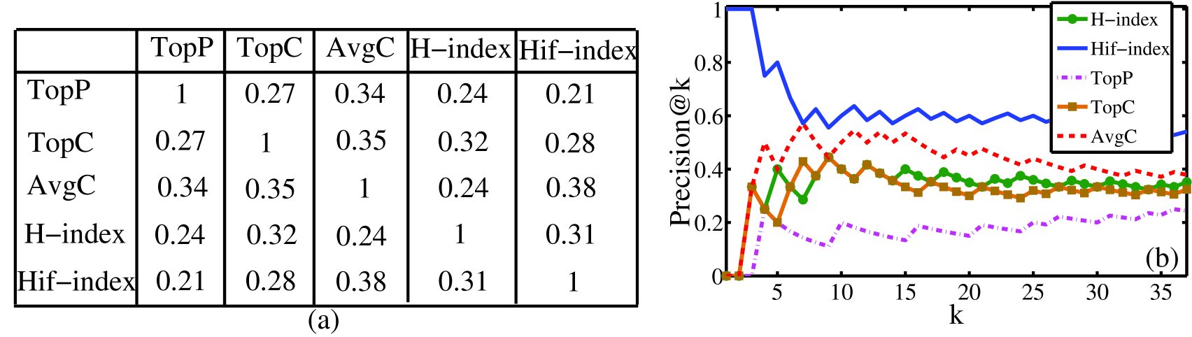
Figure 3: (a) Sprearman’s rank correlation among pair-wise ranks, and (b) the performance of all the measures.

6.3 Effect on Recommendation System

Here we show the effectiveness of reference-intensity by applying it to a real paper recommendation system. To this end, we consider FeRoSA [Chakraborty et al., 2016], a new (probably the first) framework of faceted recommendation for scientific articles, where given a query it provides facet-wise recommendations with each facet representing the purpose of recommendation [Chakraborty et al., 2016]. The methodology is based on random walk with restarts (RWR) initiated from a query paper. The model is built on AAN dataset and considers both the citation links and the content information to produce the most relevant results. Instead of using the unweighted citation network, here we use the weighted network with each edge labeled by the intensity score. The final recommendation of FeRoSA is obtained by performing RWR with the transition probability proportional to the edge-weight (we call it Inf-FeRoSA). We observe that Inf-FeRoSA achieves an average precision of $0.81$ at top 10 recommendations, which is 14% higher then FeRoSA while considering the flat version and 12.34% higher than FeRoSA while considering the faceted version.

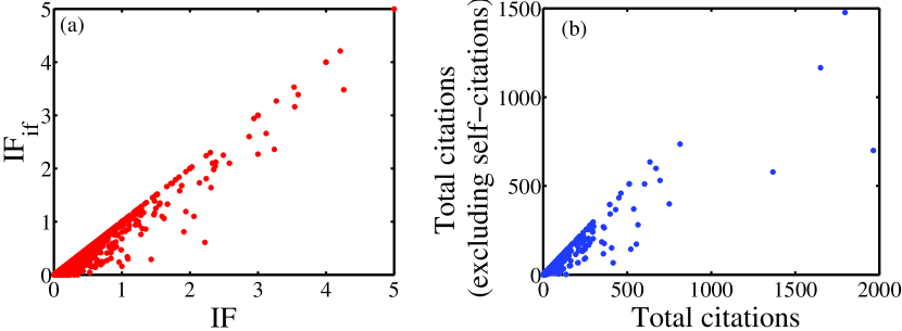
Figure 4: Correlation between (a) $IF$ and $IF_{if}$ and (b) number of citations before and after removing self-journal citations.

6.4 Detecting Citation Stacking

Recently, Thomson Reuters began screening for journals that exchange large number of anomalous citations with other journals in a cartel-like arrangement, often known as “citation stacking” [Jump, 2013, Hardcastle, 2015]. This sort of citation stacking is much more pernicious and difficult to detect. We anticipate that this behavior can be detected by the reference intensity. Since the AAN dataset does not have journal information, we use DBLP dataset [Singh et al., 2015] where the complete metadata information (along with reference contexts and abstract) is available, except the full content of the paper (559,338 papers and 681 journals; more details in [Chakraborty et al., 2014]). From this dataset, we extract all the features mentioned in Section 3.3 except the ones that require full text, and run our model using the existing annotated dataset as training instances. We measure the traditional impact factor ($IF$) of the journals and impact factor after considering the reference intensity ($IF_{if}$). Figure 4(a) shows that there are few journals whose $IF_{if}$ significantly deviates (3$\sigma$ from the mean) from $IF$; out of the suspected journals 70% suffer from the effect of self-journal citations as well (shown in Figure 4(b)), example including Expert Systems with Applications (current $IF$ of $2.53$). One of the future work directions would be to predict such journals as early as possible after their first appearance.

7 Related Work

Although the citation count based metrics are widely accepted [Garfield, 2006, Hirsch, 2010], the belief that mere counting of citations is dubious has also been a subject of study [Chubin and Moitra, 1975]. [Garfield, 1964] was the first who explained the reasons of citing a paper. [Pham and Hoffmann, 2003] introduced a method for the rapid development of complex rule bases for classifying text segments. [Dong and Schäfer, 2011] focused on a less manual approach by learning domain-insensitive features from textual, physical, and syntactic aspects To address concerns about h-index, different alternative measures are proposed [Waltman and van Eck, 2012]. However they too could benefit from filtering or weighting references with a model of influence. Several research have been proposed to weight citations based on factors such as the prestige of the citing journal [Ding, 2011, Yan and Ding, 2010], prestige of an author [Balaban, 2012], frequency of citations in citing papers [Hou et al., 2011]. Recently, [Wan and Liu, 2014] proposed a SVR based approach to measure the intensity of citations. Our methodology differs from this approach in at lease four significant ways: (i) they used six very shallow level features; whereas we consider features from different dimensions, (ii) they labeled the dataset by the help of independent annotators; here we additionally ask the authors of the citing papers to identify the influential references which is very realistic [Gilbert, 1977]; (iii) they adopted SVR for labeling, which does not perform well for small training instances; here we propose GraLap , designed specifically for small training instances; (iv) four applications of reference intensity mentioned here are completely new and can trigger further to reassessing the existing bibliometrics.

8 Conclusion

We argued that the equal weight of all references might not be a good idea not only to gauge success of a research, but also to track follow-up work or recommending research papers. The annotated dataset would have tremendous potential to be utilized for other research. Moreover, GraLap  can be used for any semi-supervised learning problem. Each application mentioned here needs separate attention. In future, we shall look into more linguistic evidences to improve our model.

References

- [Athar and Teufel, 2012] Awais Athar and Simone Teufel. 2012. Context-enhanced citation sentiment detection. In NAACL, pages 597–601, Stroudsburg, PA, USA. ACL.
- [Balaban, 2012] Alexandru T. Balaban. 2012. Positive and negative aspects of citation indices and journal impact factors. Scientometrics, 92(2):241–247.
- [Berger et al., 1996] Adam L. Berger, Vincent J. Della Pietra, and Stephen A. Della Pietra. 1996. A maximum entropy approach to natural language processing. Comput. Linguist., 22(1):39–71, March.
- [Chakraborty et al., 2014] Tanmoy Chakraborty, Suhansanu Kumar, Pawan Goyal, Niloy Ganguly, and Animesh Mukherjee. 2014. Towards a stratified learning approach to predict future citation counts. In Proceedings of the 14th ACM/IEEE-CS Joint Conference on Digital Libraries, JCDL ’14, pages 351–360, Piscataway, NJ, USA. IEEE Press.
- [Chakraborty et al., 2016] Tanmoy Chakraborty, Amrith Krishna, Mayank Singh, Niloy Ganguly, Pawan Goyal, and Animesh Mukherjee, 2016. Advances in Knowledge Discovery and Data Mining: 20th Pacific-Asia Conference, PAKDD 2016, Auckland, New Zealand, April 19-22, 2016, Proceedings, Part II, chapter FeRoSA: A Faceted Recommendation System for Scientific Articles, pages 528–541. Springer International Publishing, Cham.
- [Chodorow and Leacock, 2000] Martin Chodorow and Claudia Leacock. 2000. An unsupervised method for detecting grammatical errors. In NAACL, pages 140–147, Stroudsburg, PA, USA. Association for Computational Linguistics.
- [Chubin and Moitra, 1975] D. E. Chubin and S. D. Moitra. 1975. Content-Analysis of References – Adjunct or Alternative to Citation Counting. Social studies of science, 5(4):423–441.
- [Cohen, 1960] J. Cohen. 1960. A Coefficient of Agreement for Nominal Scales. Educational and Psychological Measurement, 20(1):37–41.
- [Councill et al., 2008] Isaac G Councill, C Lee Giles, and Min-Yen Kan. 2008. Parscit: an open-source crf reference string parsing package. In LREC, pages 28–30, Marrakech, Morocco.
- [Ding, 2011] Ying Ding. 2011. Applying weighted pagerank to author citation networks. JASIST, 62(2):236–245.
- [Dong and Schäfer, 2011] Cailing Dong and Ulrich Schäfer. 2011. Ensemble-style self-training on citation classification. In IJCNLP, pages 623–631. ACL, 11.
- [Dubin, 2004] David Dubin. 2004. The most influential paper gerard salton never wrote. Library Trends, 52(4):748–764.
- [Garfield, 1964] Eugene Garfield. 1964. Can citation indexing be automated? Statistical association methods for mechanized documentation, Symposium proceedings, pages 188–192.
- [Garfield, 2006] Eugene Garfield. 2006. The History and Meaning of the Journal Impact Factor. JAMA, 295(1):90–93.
- [Gilbert, 1977] G. N. Gilbert. 1977. Referencing as persuasion. Social Studies of Science, 7(1):113–122.
- [Hardcastle, 2015] James Hardcastle. 2015. Citations, self-citations, and citation stacking, http://editorresources.taylorandfrancisgroup.com/citations-self-citations\\-and-citation-stacking/.
- [Hirsch, 2005] J. E. Hirsch. 2005. An index to quantify an individual’s scientific research output. PNAS, 102(46):16569–16572.
- [Hirsch, 2010] J. E. Hirsch. 2010. An index to quantify an individual’s scientific research output that takes into account the effect of multiple coauthorship. Scientometrics, 85(3):741–754, December.
- [Hou et al., 2011] Wen-Ru Hou, Ming Li, and Deng-Ke Niu. 2011. Counting citations in texts rather than reference lists to improve the accuracy of assessing scientific contribution. BioEssays, 33(10):724–727.
- [Jochim and Schütze, 2012] Charles Jochim and Hinrich Schütze. 2012. Towards a generic and flexible citation classifier based on a faceted classification scheme. In COLING, pages 1343–1358, Bombay, India.
- [Jump, 2013] Paul Jump. 2013. Journal citation cartels on the rise, https://www.timeshighereducation.com/news/journal-citation-cartels-on-the-rise/2005009.article.
- [Kruskal, 1956] J. B. Kruskal. 1956. On the Shortest Spanning Subtree of a Graph and the Traveling Salesman Problem. In Proceedings of the American Mathematical Society, volume 7, pages 48–50.
- [Liakata et al., 2012] Maria Liakata, Shyamasree Saha, Simon Dobnik, Colin R. Batchelor, and Dietrich Rebholz-Schuhmann. 2012. Automatic recognition of conceptualization zones in scientific articles and two life science applications. Bioinformatics, 28(7):991–1000.
- [Marneffe et al., 2006] M. Marneffe, B. Maccartney, and C. Manning. 2006. Generating typed dependency parses from phrase structure parses. In LREC, pages 449–454, Genoa, Italy, May. European Language Resources Association (ELRA).
- [Moravcsik and Murugesan, 1975] M. J. Moravcsik and P. Murugesan. 1975. Some results on the function and quality of citations. Social studies of science, 5(1):86–92.
- [Page et al., 1998] L. Page, S. Brin, R. Motwani, and T. Winograd. 1998. The pagerank citation ranking: Bringing order to the web. In WWW, pages 161–172, Brisbane, Australia.
- [Pham and Hoffmann, 2003] Son Bao Pham and Achim Hoffmann. 2003. A new approach for scientific citation classification using cue phrases. In Tamas Domonkos Gedeon and Lance Chun Che Fung, editors, Advances in Artificial Intelligence: 16th Australian Conference on AI, pages 759–771. Springer Berlin Heidelberg.
- [Porter, 1997] M. F. Porter. 1997. Readings in information retrieval. chapter An Algorithm for Suffix Stripping, pages 313–316. Morgan Kaufmann Publishers Inc., San Francisco, CA, USA.
- [Pukelsheim, 1994] Friedrich Pukelsheim. 1994. The Three Sigma Rule. The American Statistician, 48(2):88–91.
- [Pustejovsky et al., 1993] James Pustejovsky, Peter Anick, and Sabine Bergler. 1993. Lexical semantic techniques for corpus analysis. Comput. Linguist., 19(2):331–358, June.
- [Quinlan, 1993] J. Ross Quinlan. 1993. C4.5: Programs for Machine Learning. Morgan Kaufmann Publishers Inc., San Francisco, CA, USA.
- [Radev et al., 2009] Dragomir R. Radev, Pradeep Muthukrishnan, and Vahed Qazvinian. 2009. The acl anthology network corpus. In Proceedings of the 2009 Workshop on Text and Citation Analysis for Scholarly Digital Libraries, NLPIR4DL, pages 54–61, Stroudsburg, PA, USA. ACL.
- [Simkin and Roychowdhury, 2003] Mikhail V. Simkin and V. P. Roychowdhury. 2003. Read Before You Cite! Complex Systems, 14:269–274.
- [Singh et al., 2015] Mayank Singh, Vikas Patidar, Suhansanu Kumar, Tanmoy Chakraborty, Animesh Mukherjee, and Pawan Goyal. 2015. The role of citation context in predicting long-term citation profiles: An experimental study based on a massive bibliographic text dataset. In CIKM, pages 1271–1280, New York, NY, USA. ACM.
- [Small, 1973] Henry Small. 1973. Co-citation in the scientific literature: A new measure of the relationship between two documents. JASIST, 24(4):265–269.
- [Teufel et al., 2006] Simone Teufel, Advaith Siddharthan, and Dan Tidhar. 2006. Automatic classification of citation function. In EMNLP, pages 103–110, Stroudsburg, PA, USA. ACL.
- [Toutanova and Manning, 2000] Kristina Toutanova and Christopher D. Manning. 2000. Enriching the knowledge sources used in a maximum entropy part-of-speech tagger. In EMNLP, pages 63–70, Stroudsburg, PA, USA. ACL.
- [Turney and Pantel, 2010] Peter D. Turney and Patrick Pantel. 2010. From frequency to meaning: Vector space models of semantics. J. Artif. Int. Res., 37(1):141–188, January.
- [Waltman and van Eck, 2012] Ludo Waltman and Nees Jan van Eck. 2012. The inconsistency of the h-index. JASIST, 63(2):406–415, February.
- [Wan and Liu, 2014] Xiaojun Wan and Fang Liu. 2014. Are all literature citations equally important? automatic citation strength estimation and its applications. JASIST, 65(9):1929–1938.
- [Witten and Frank, 2005] Ian H. Witten and Eibe Frank. 2005. Data Mining: Practical Machine Learning Tools and Techniques, Second Edition (Morgan Kaufmann Series in Data Management Systems). Morgan Kaufmann Publishers Inc., San Francisco, CA, USA.
- [Yan and Ding, 2010] Erjia Yan and Ying Ding. 2010. Weighted citation: An indicator of an article’s prestige. JASIST, 61(8):1635–1643.
- [Zhu et al., 2003] Xiaojin Zhu, Zoubin Ghahramani, and John Lafferty. 2003. Semi-supervised learning using gaussian fields and harmonic functions. In ICML, pages 912–919, Washington D.C.
- [Zhu et al., 2015] Xiaodan Zhu, Peter Turney, Daniel Lemire, and André Vellino. 2015. Measuring academic influence: Not all citations are equal. JASIST, 66(2):408–427.