Cost-effective description of strong correlation: efficient implementations of the perfect quadruples and perfect hextuples models

Abstract

Novel implementations based on dense tensor storage are presented for the singlet-reference perfect quadruples (PQ) [Parkhill, Lawler, and Head-Gordon, J. Chem. Phys. 130, 084101 (2009)] and perfect hextuples (PH) [Parkhill and Head-Gordon, J. Chem. Phys. 133, 024103 (2010)] models. The methods are obtained as block decompositions of conventional coupled-cluster theory that are exact for four electrons in four orbitals (PQ) and six electrons in six orbitals (PH), but that can also be applied to much larger systems. PQ and PH have storage requirements that scale as the square, and as the cube of the number of active electrons, respectively, and exhibit quartic scaling of the computational effort for large systems. Applications of the new implementations are presented for full-valence calculations on linear polyenes (C_nH_n+2), which highlight the excellent computational scaling of the present implementations that can routinely handle active spaces of hundreds of electrons. The accuracy of the models is studied in the $\pi$ space of the polyenes, in hydrogen chains (H50), and in the $\pi$ space of polyacene molecules. In all cases, the results compare favorably to density matrix renormalization group values. With the novel implementation of PQ, active spaces of 140 electrons in 140 orbitals can be solved in a matter of minutes on a single core workstation, and the relatively low polynomial scaling means that very large systems are also accessible using parallel computing.

I Introduction

Efficient handling of strong correlation is one of the still unresolved questions in computational chemistry. Outside the scope of the otherwise useful Kohn–Sham density-functional theory(Hohenberg and Kohn, 1964; Kohn and Sham, 1965; Kurzweil et al., 2009), approaches to strong correlation lean heavily on wave function theories. The conventional way to treat strong correlation is through multiconfigurational self-consistent field (MCSCF) theory, which scales exponentially as the size of the active space grows. As a result, MCSCF cannot be applied to active spaces significantly larger than 16 electrons in 16 orbitals, although the barrier has been recently pushed back through approximative stochastic(Thomas et al., 2015; Manni et al., 2016) and adaptive(Schriber and Evangelista, 2016; Tubman et al., 2016; Liu and Hoffmann, 2016; Zhang and Evangelista, 2016; Holmes et al., 2016) approaches to the full configuration interaction (FCI) problem.

Now, while MCSCF relies on a configuration interaction (CI) type ansatz $\Ket{\Psi}=(1+\hat{T})\Ket{\Phi}$ for the wave function, where $\Ket{\Phi}$ is the single-particle reference and $\Ket{\Psi}$ the true, multiconfigurational wave function, one might ask whether a coupled-cluster(Čížek, 1966) (CC) type ansatz $\Ket{\Psi}=\exp(\hat{T})\Ket{\Phi}$ could be used instead to formulate a MCSCF-type model. The CC approach can also be used to describe dynamic correlation with a CI reference, as in the multireference CC (MR-CC) approach(Lyakh et al., 2012), but MR-CC is much more complicated than single-reference CC, and combining both strong correlation and dynamic correlation within the same machinery would be clearly advantageous. While in principle CC theory is well able to describe static correlation, the problem that arises upon its application is that the computational effort of the resulting procedure is prohibitively expensive, even if an active space is used(Krylov et al., 1998). However, this problem has been recently solved by Parkhill, Lawler, and Head-Gordon, who proposed a truncation of CC for exactness within the active space for a given number of strongly interacting electron pairs(Parkhill et al., 2009; Parkhill and Head-Gordon, 2010a), instead of the usual, global truncation based on the excitation level. For example, the perfect quadruples(Parkhill et al., 2009) (PQ) model is formed by truncating CC theory with single through quadruple (CCSDTQ) excitations to two pairs by keeping only the amplitudes $t_{i_{1}\dots i_{n}}^{a_{1}\dots a_{n}}$ that satisfy $\{a_{k},i_{k}\}\in\{\text{pair}_{1}\}\times\{\text{pair}_{2}\}$. Similarly, the perfect hextuples(Parkhill and Head-Gordon, 2010a) (PH) model is a three-pair truncation of CC theory with single through hextuple excitations (CCSDTQ56), in which only the amplitudes that satisfy $\{a_{k},i_{k}\}\in\{\text{pair}_{1}\}\times\{\text{pair}_{2}\}\times\{\text{pair}_{3}\}$ are kept. Here, the concept of a pair arises from connection to the perfect pairing(Hurley et al., 1953; Hunt et al., 1972; Ukrainskii, 1977; Goddard and Harding, 1978; Cullen, 1996) (PP) theory, in which pair $i$ is described by a quartet of orbitals: the alpha and beta orbitals $i$ and $\bar{i}$, respectively, that are occupied in the single-particle reference, as well as the corresponding alpha and beta virtual orbitals $i^{*}$ and $\bar{i}^{*}$, respectively. In contrast to MCSCF, PQ and PH exhibit polynomial scaling with respect to the size of the active space. The storage requirements are modest, scaling as $O(N^{2})$ for PQ and $O(N^{3})$ for PH, $N$ being the number of active orbitals in the calculation. The computational effort scales asymptotically as $O(N^{4}$) for both models.

Another widely used approach for strong correlation is the density matrix renormalization group (DMRG) method(White, 1992; Chan et al., 2008; Marti and Reiher, 2010; Wouters and Van Neck, 2014; Olivares-Amaya et al., 2015), which is exact in principle and which also offers polynomial scaling with respect to system size. However, the method has a significant prefactor: the storage and computational costs scale as(Hachmann et al., 2006; Olivares-Amaya et al., 2015) $O(M^{2}N^{3})$ and $O(M^{3}N^{3})+O(M^{2}N^{4})$, respectively, where $M$ is the number of states kept in the calculation. Furthermore, as a fundamentally one-dimensional approach, DMRG has a history of being hard to use due to issues with orbital ordering, although automatic orbital ordering schemes have recently made DMRG calculations easier to perform. We note that other approaches for a compact description of strong correlation have also been suggested, such as the CC valence bond (CCVB) method(Small and Head-Gordon, 2009, 2011; Small et al., 2014), extended CC(Arponen, 1983; Arponen et al., 1987a, b), and the multifacet graphically contracted function method(Shepard et al., 2014a, b).

In order to apply MCSCF, DMRG, PQ, or PH to studies of chemical systems, the additional description of dynamic correlation is usually of utmost importance. While MCSCF and DMRG typically rely on a two-pronged approach to dynamic correlation through CI, CC, or perturbative approaches, dynamic correlation can be treated on the same footing as static correlation in PQ and PH(Parkhill and Head-Gordon, 2010b), enabling the two types of correlation to interact. Note that perturbative approaches can be used as well in combination with PQ(Parkhill et al., 2011) and PH.

What unites MCSCF, DMRG, PQ, and PH is that the choice of the set of active orbitals is a problem, and often the orbitals need to be optimized in order to fully capture static correlation effects. Orbital optimization is hard for PQ and PH, but earlier experience(Parkhill and Head-Gordon, 2010a) suggests that in many cases orbitals optimized at the much simpler PP level of theory might be sufficient for a wide variety of applications. Thus, in the present work, only localized Hartree–Fock orbitals and PP optimized orbitals will be considered. Orbitals optimized with CCVB, or unrestricted Hartree–Fock natural orbitals(Pulay and Hamilton, 1988; Bofill and Pulay, 1989; Keller et al., 2015) might also prove useful. However, because the feasible size of the active space is much larger in PQ and PH than in MCSCF or even DMRG, it is likely that for full-valence calculations the choice of the active space orbitals should not prove to be an impediment to the use of the PQ and PH models.

While encouraging results have been achieved withPQ and PH, their existing implementations (while exhibiting the correct $O(N^{4})$ scaling with system size) have a too large prefactor to allow their application to studies of chemical problems. Because the previous implementations are based on the use of sparse tensor algebra(Parkhill and Head-Gordon, 2010c), it is worth asking if the prefactor could be reduced by the use of dense tensor storage, instead. Moreover, the existing sparse tensor implementation does not take advantage of the mathematical structure of the PQ and PH methods, which results in extra work for bookkeeping and prevents efficient compiler optimization from taking place.

In the present work, we describe the dense tensor implementation of the PQ and PH models, and benchmark the resulting code against the previous implementation on linear polyenes. Novel applications of the PQ and PH models are demonstrated for the H50 chain, and the results are compared to DMRG. Applications of PQ and PH to the strongly correlated $\pi$ space of the polyacene series are also presented. The organization of the manuscript is the following. In the Theory section, we illustrate how the truncation of CC theory is performed. Next, in the Implementation section, we describe various aspects of how the procedure has been carried out in practice. In the Results section we present the scaling of the new code when applied to linear polyenes, and the energies for the polyenes, the dissociation of the H50 chain, as well as the polyacenes for which natural occupation numbers are also presented. The study concludes with a summary and brief discussion.

II Theory

Figure 1: Division of the orbital space. The active space orbitals are numbered with the value of the pairing label. The hole indices are reversed, because the strongest coupling typically occurs between the highest occupied and lowest unoccupied orbitals.

The theory behind the CC approach is well established and shall not be discussed further here(Crawford and Schaefer, 2000; Bartlett and Musiał, 2007). The starting point for the present truncation are the CC equations in spin-integrated form, consisting of tensors that belong to a certain spin block, such as the $\alpha\beta$ block of the double excitation amplitudes, where $\alpha$ and $\beta$ denote spin-up and spin-down, respectively. As a truncation of CC theory, the models in the present hierarchy inherit all the beneficial properties of CC such as size extensivity, but also its drawbacks such as non-variational behavior in cases where the excitation rank in CC is not high enough to describe the static correlation effects.

In the following we will omit the spin indices, because the discussion applies to all tensors that appear in CC theory. We will mostly be focusing on the PQ model, as it already illustrates all of the necessary aspects for a general truncation method without being overly complicated. The division of the orbital space that is used in the present work is illustrated in 1. The system, in a singlet reference state, is composed of a set of inactive core orbitals, a set of $N$ active occupied orbitals, a set of $N$ active virtual orbitals, and a set of inactive virtual orbitals. The tensors, such as the excitation amplitudes $t$, the two-electron integrals $v$, the de-excitation amplitudes $\lambda$ and the one- and two-electron density matrices $\gamma$ and $\Gamma$ are truncated using a block decomposition. For instance, for PQ it is not hard to see that the expansion of the double excitation tensor as

$$t_{ij}^{ab}= \sum_{P=1}^{N}t_{PP}^{PP}\delta_{iP}\delta_{jP}\delta_{aP}\delta_{bP}+\sum_{\begin{subarray}{c}P,Q=1\\ P\neq Q\end{subarray}}^{N}t_{PP}^{PQ}\delta_{iP}\delta_{jP}\delta_{aP}\delta_{bQ}+\sum_{\begin{subarray}{c}P,Q=1\\ P\neq Q\end{subarray}}^{N}t_{PP}^{QP}\delta_{iP}\delta_{jP}\delta_{aQ}\delta_{bP}+\sum_{\begin{subarray}{c}P,Q=1\\ P\neq Q\end{subarray}}^{N}t_{PQ}^{PP}\delta_{iP}\delta_{jQ}\delta_{aP}\delta_{bP}$$ (1)

$$+ \sum_{\begin{subarray}{c}P,Q=1\\ P\neq Q\end{subarray}}^{N}t_{QP}^{PP}\delta_{iQ}\delta_{jP}\delta_{aP}\delta_{bP}+\sum_{\begin{subarray}{c}P,Q=1\\ P\neq Q\end{subarray}}^{N}t_{PQ}^{PQ}\delta_{iP}\delta_{jQ}\delta_{aP}\delta_{bQ}+\sum_{\begin{subarray}{c}P,Q=1\\ P\neq Q\end{subarray}}^{N}t_{QP}^{PQ}\delta_{iQ}\delta_{jP}\delta_{aP}\delta_{bQ}+\sum_{\begin{subarray}{c}P,Q=1\\ P\neq Q\end{subarray}}^{N}t_{PP}^{QQ}\delta_{iP}\delta_{jP}\delta_{aQ}\delta_{bQ}$$

where $i$ and $j$ denote occupied orbitals, $a$ and $b$ denote virtual orbitals, $P$ and $Q$ are pairing labels that run over the active space and $\delta_{PQ}$ is the Kronecker delta is equivalent to the original definition of the PQ model as the set of amplitudes $t_{i_{1}\dots i_{n}}^{a_{1}\dots a_{n}}$ that satisfy $\{a_{k},i_{k}\}\in\{\text{pair}_{1}\}\times\{\text{pair}_{2}\}$. As this kind of notation is unusual to most chemists, we will try to clarify the meaning of (LABEL:decompose) in the following. In the convention adapted above, all the orbitals in the alpha and beta occupied and virtual spaces are numbered from 1 to $N$, which is also the range spanned by the pairing labels. Because we have assumed that the spin has been integrated out, all the quantities in (LABEL:decompose) are scalar numbers. The indices $i,j,a,b$ are fixed by the left hand side of the equation, which represents the element of the excitation tensor under decomposition. The Kronecker delta is defined as $\delta_{ij}=1$ when $i=j$ and $\delta_{ij}=0$ when $i\neq j$. Applying the decomposition to, for example, the element $t_{kk}^{cc}$ with $k\neq c$ will only yield a contribution from the last term of (LABEL:decompose) (which equals $t_{kk}^{cc}$), because the first term would require $k=c$ and all the other terms would contribute only for $P=Q$ which has been excluded in the summations.

The restriction to identically sized active occupied and virtual spaces becomes apparent here, as the same pairing labels cannot be used for spaces of different size. Each value of a pairing label corresponds to a quartet of orbitals: the alpha and beta occupied orbital, and the alpha and beta virtual orbital. The tensor decomposition in (LABEL:decompose) is known in mathematics as a block decomposition(De Lathauwer, 2008a, b). For PH, in addition to the 8 cases shown in (LABEL:decompose) one obtains 63 more, corresponding to all the inequivalent ways of distributing three labels to four indices: for instance, $t_{QQ}^{QP}$ is equivalent to $t_{PP}^{PQ}$ as the dummy summation indices $P$ and $Q$ can be interchanged. Having enumerated the different subtensor representations for all the necessary tensors, one proceeds by inserting them into the CC equations and by performing the summations over the Kronecker deltas. When this is done, one ends up with a formulation of PQ or PH theory in terms of the dense subtensors. For example, in the case of PH the original hextuple excitation operator $T_{ijklmn}^{abcdef}$, which is a rank-12 tensor, is reduced to a set of rank-3 tensors, and any summations that are left over are only with respect to the pairing labels. While in principle, the doubles contribution to the opposite spin correlation energy

$$E_{c}\leftarrow \sum_{ijab}t_{ij}^{ab}v_{ij}^{ab}$$ (2)

has $8\times 8=64$ distinct subtensor contributions in PQ (and 5041 in PH), it is seen that due to orthogonality of the Kronecker indices the PQ expression becomes simply

$$E_{c}\leftarrow \sum_{P}t_{PP}^{PP}v_{PP}^{PP}+\sum_{\begin{subarray}{c}P,Q=1\\ P\neq Q\end{subarray}}^{N}t_{PP}^{PQ}v_{PP}^{PQ}+\sum_{\begin{subarray}{c}P,Q=1\\ P\neq Q\end{subarray}}^{N}t_{PP}^{QP}v_{PP}^{QP}+\sum_{\begin{subarray}{c}P,Q=1\\ P\neq Q\end{subarray}}^{N}t_{PQ}^{PP}v_{PQ}^{PP}$$ (3)

$$+ \sum_{\begin{subarray}{c}P,Q=1\\ P\neq Q\end{subarray}}^{N}t_{QP}^{PP}v_{QP}^{PP}+\sum_{\begin{subarray}{c}P,Q=1\\ P\neq Q\end{subarray}}^{N}t_{PQ}^{PQ}v_{PQ}^{PQ}+\sum_{\begin{subarray}{c}P,Q=1\\ P\neq Q\end{subarray}}^{N}t_{QP}^{PQ}v_{QP}^{PQ}+\sum_{\begin{subarray}{c}P,Q=1\\ P\neq Q\end{subarray}}^{N}t_{PP}^{QQ}v_{PP}^{QQ}.$$

The limitation to $P\neq Q$ in (LABEL:energy-contr) and similar equations can be easily lifted by establishing a convention in which all diagonals of the subtensors vanish.

One can identify a set of 8 subtensors in (LABEL:decompose,energy-contr): $t_{PP}^{PP}(P)$, $t_{PP}^{PQ}(P,Q)$, $t_{PP}^{QP}(P,Q)$, $t_{PQ}^{PP}(P,Q)$, $t_{QP}^{PP}(P,Q)$, $t_{PQ}^{PQ}(P,Q)$, $t_{QP}^{PQ}(P,Q)$, and $t_{PP}^{QQ}(P,Q)$. The first term in (LABEL:decompose), $t_{PP}^{PP}(P)$ can be identified as the PP amplitude (singles are usually not included in the definition of PP as the orbitals are normally optimized). As the simplest truncation (exactness for two electrons in two orbitals), PP has a special place within the hierarchy of the truncated models. Because PP couples every occupied orbital to a specific virtual orbital, the amplitudes are independent and can be solved for in closed form. Orbital optimization can then be done in a routine fashion even for large systems(Beran et al., 2005). The terms $t_{PP}^{PP}(P)$, $t_{PQ}^{PQ}(P,Q)$, and $t_{QP}^{PQ}(P,Q)$ in (LABEL:decompose) are the basis of the imperfect pairing (IP) model(Van Voorhis and Head-Gordon, 2000), which is considerably more complicated than PP but has still been originally been derived by hand, and for which orbital optimization is still a routine task.

However, in addition to the terms in (LABEL:decompose) that represent double excitations, PQ also includes single, triple, and quadruple excitations, and unlike PP and IP is not restricted to opposite-spin correlation, so the derivation of the equations for PQ would be a challenging task by hand. Fortunately, it is an ideal task for a computer.

Antisymmetricity between same-spin indices can be used to eliminate redundant storage of equivalent contributions (e.g., $t_{PQ}^{QP}=-t_{PQ}^{PQ}$ for the $\alpha\alpha$ and $\beta\beta$ blocks in (LABEL:decompose)). The resulting storage costs for the subtensors that appear at the PP, PQ, and PH levels of theory are shown in 1. For instance, for PQ the storage cost is $17N^{2}+3N$ for the amplitudes, $113N^{2}+19N$ for the density matrices and $115N^{2}+23N$ for the integrals. The figures in 1 also include the classes of integrals that are only needed for the calculation of the CC pseudoenergy; for a $t$ amplitude-only program the amount of integrals would be slightly smaller. noamps details the distribution of the total amplitude subtensors into the individual excitation ranks.

Due to the truncation of the amplitudes and integrals, PP, PQ, and PH are not invariant to rotations in the occupied–occupied or virtual–virtual blocks, unlike their parent CC theories. The same will also apply perfect octuples (PO) theory, which would be a truncation of CC theory with single through octuple excitations (CCSDTQ5678) based on exactness for eight electrons in eight orbitals. This is somewhat counterintuitive, because in contrast to PP, PQ, and PH, the full set of one- and two-electron integrals is used in PO, encoding in principle all there is to know about the system. But, the triple through octuple excitation operators would still not be fully described within PO, and the truncation is based on orbital labels, so the used set of orbitals would still be an issue in PO. However, seeing as the issues with the choice of orbitals clearly ease up going from PP to PQ to PH, PO might not be very sensitive to the orbitals after all.

Due to the one-to-one coupling of occupied and virtual orbitals PP (and IP) is obviously dependent on the relative ordering of the occupied and virtual orbitals. But, the same property also applies to the PQ and PH models. For instance, if one interchanges the virtual orbitals 2 and 3, the PQ doubles amplitude $t_{12}^{12}$ in the original numbering would become $t_{12}^{13}$ in the renumbered system. However, $t_{12}^{13}$ is not included in the PQ model, so the description of the system has changed. By a similar analysis, it is easy to see that the dependence on the orbital orderings holds for all tensors that are truncated in the subtensor expansion. Due to this common property, we refer to the hierarchy of the PP, PQ, and PH (and higher models) as the perfect pairing hierarchy to underline the pairing of the orbital quartets, formed of occupied and virtual alpha and beta orbitals, at each level of theory.

The origin of the dependence on the relative ordering of the occupied and virtual orbitals is easy to understand on physical grounds. In order to reduce the computational scaling, we wished to retain only the strongest interactions between orbitals. The pairing of occupied orbitals to virtual orbitals introduces a sense of locality in the model that results in fast convergence of the truncation, as in the usual local dynamic correlation methods(Pulay, 1983; Saebo and Pulay, 1993). The models in the PP hierarchy are, however, invariant to swaps between pairs (i.e. quartets) of orbitals.

The models in the PP hierarchy assume a pairing of the occupied and virtual orbitals before the calculation is began. While PP optimized orbitals will produce the best possible pairing in the sense of reproducing the lowest energy at the PP level of theory, it is not clear that the PP orbitals, which usually turn out to be local, will be optimal for the PQ or PH models: for instance in polyacenes, the optimal orbitals for CCVB (which describes more strong correlation than PP) turn out to be more delocalized than PP orbitals(Small et al., 2014). However, as stated in the Introduction, variational optimization of the orbitals for PQ and PH is hard, which means that one may need to resort to approximate methods of obtaining localized orbitals with matching virtual orbitals. But, this may not be a problem after all: while orbital optimization is necessary at the PP level of theory due its aggressive truncation (which also makes the optimization problem tractable), it is plausible that the use of optimal orbitals is less important at higher levels of the hierarchy, because at every step the models become closer to FCI which is orbital invariant. In analogy to local dynamic correlation methods, reasonable orbitals can be obtained from a Hartree–Fock or density-functional theory calculation by localizing the occupied orbitals using, e.g., the Foster–Boys(Foster and Boys, 1960) (FB), Edmiston–Ruedenberg(Edmiston and Ruedenberg, 1963) (ER), or Pipek–Mezey(Pipek and Mezey, 1989; Lehtola and Jónsson, 2014) (PM) criteria, after which matching virtual orbitals can be obtained, e.g., by using the Sano procedure(Sano, 2000). In the present work, both PP orbitals and Pipek–Mezey orbitals are used.

	rank-1	rank-2	rank-3
$t$/$\lambda$	3	17	64
$f$	10	6	0
$v$	13	109	96
$\gamma$	6	6	0
$\Gamma$	13	107	96

Table 1: Storage costs for the $t$ and $\lambda$ amplitudes, one-electron integrals $f$, two-electron integrals $v$, and one- and two-particle density matrices $\gamma$ and $\Gamma$, respectively, that appear in unrestricted PP, PQ, and PH. PP includes all rank-1 subtensors, PQ includes all rank-1 and rank-2 subtensors and PH includes all rank-1 through rank-3 subtensors.

	rank-1	rank-2	rank-3
$T_{1}/\Lambda_{1}$	2	2
$T_{2}/\Lambda_{2}$	1	9	8
$T_{3}/\Lambda_{3}$		5	29
$T_{4}/\Lambda_{4}$		1	21
$T_{5}/\Lambda_{5}$			5
$T_{6}/\Lambda_{6}$			1

Table 2: Number of amplitude subtensors at different levels of truncation, including all spin blocks. PP includes all rank-1 subtensors, PQ includes all rank-1 and rank-2 subtensors and PH includes all rank-1 through rank-3 subtensors.

III Implementation

We have written a C++ program that generates C++ source code for the PP, PQ, and PH models, starting from CC equations in spin-orbital form. In the generated code, the subtensors are stored in memory separately as arrays. Subtensor symmetry, like $t_{PQ}^{PQ}(P,Q)=t_{PQ}^{PQ}(Q,P)$ for the same-spin doubles excitation amplitudes, is not used in the storage. As is usual for CC theory, the implementation bases on the use of intermediates in evaluating nested tensor products, such as in the singles contribution to the doubles amplitude

$$t_{ij}^{ab}\leftarrow \sum_{klcd}t_{k}^{a}t_{l}^{b}t_{i}^{c}t_{j}^{d}v_{kl}^{cd}.$$

Pairings are also generated for the intermediates, and the index antisymmetries of the intermediates are used to eliminate labelings vanishing by Pauli exclusion. The truncation of the intermediates and integrals is controlled separately from that of the excitation amplitudes. For PQ, the intermediates can be truncated to either 2 or 3 pairs, while for PH a 3-pair truncation is always used. As a result, the solution of PQ will scale as $O(N^{3})$ or $O(N^{4})$, depending on which truncation is used, and PH will also scale as $O(N^{4})$. In the present work, both PQ and PH use 3-pair intermediates, yielding asymptotic $O(N^{4})$ scaling for both models.

The program performs the pairings by brute force by looping over all the necessary index permutations of the amplitude diagrams in spin-orbital form, performing the integration over spin into different spin blocks, and performing the pairing for each block separately. The generation of the PQ model was found to take roughly 3 minutes on a single core of a workstation, while generation of the PH model took 14.5 days on 32 cores on a cluster node. Almost all the time for the PH model was spent in pairing the hextuple $t$ excitation amplitudes.

The equations for the subtensor contributions are saved on disk in human-readable form. OpenMP parallellization is performed over the individual contributions. For example, the PQ model has 4529 different contributions to the $t$ amplitudes, while PH has 213234 different contributions to the $t$ amplitudes. Altogether, the generated PQ equations take 27 megabytes of disk space in 10080 files, while the PH equations take four gigabytes of disk space in almost a quarter million files.

Besides merging contributions that require identical sets of intermediates, no attempt has been made to search for an optimal reduced set of contributions. This procedure reduces the amount of separate contributions by roughly one half from the numbers given above. While common subexpression elimination techniques commonly performed in conventional CC theory could clearly be used here, it appears that because of the introduction of a large variety of subtensors, more optimal sets of intermediates could be found with a thorough graph search.

Only a single copy of the integrals is kept in memory. A disk based direct inversion in the iterative subspace(Pulay, 1980) (DIIS) approach is used to accelerate the convergence of the CC amplitudes(Scuseria et al., 1986).

In contrast to conventional CC theory, the pairing of the indices introduces elementwise (Hadamard) procucts in the pairwise tensor products. Now, while the number of permutations in a rank-$n$ tensor increases as $n!$, the number of possible products of two rank-$n$ tensors would increase as $(n!)^{2}$, which becomes unmanageable even for relatively small $n$. For this reason, our implementation is based on hardcoded C++ computation kernels for each permutationally invariant type of contribution, where indices are either fixed (output index appears only on one of the two tensors), elementwise multiplied over (output index appears on both tensors), or contraction indices (index appears on both tensors but is not an output index). The kernels are machine generated in an external library, both as a for-loop-only implementation, and as code calling basic linear algebra subprogram (BLAS) routines wherever applicable. When the library is generated, the two kinds of implementations are benchmarked to determine which one to use for a given kernel.

The two-electron integrals are evaluated in the program from B matrices that can be generated by the resolution of the identity(Vahtras et al., 1993) (RI) or Cholesky decomposition(Beebe and Linderberg, 1977) (CD) techniques, as their integral transforms scale more favorably than that of the traditional two-electron integrals, and as the RI/CD representation allows for cherrypicking of the wanted integral elements. The Fock and RI/CD B matrices may currently be obtained from either Q-Chem(Epifanovsky et al., 2013; Shao et al., 2014) or ERKALE(Lehtola et al., 2012; Lehtola, 2016). Both programs have been utilized in the present work: Q-Chem for calculations using PP orbitals, and ERKALE for calculations with localized Hartree–Fock orbitals. In the latter case, the active occupied orbitals are localized using the generalized Pipek–Mezey method(Lehtola and Jónsson, 2014) using the intrinsic atomic orbital partial charge estimate(Knizia, 2013). The gradient descent method used for the localization has been described elsewhere(Lehtola and Jónsson, 2013). After the occupied space has been localized, corresponding virtual orbitals are obtained for each active occupied orbital using the Sano procedure(Sano, 2000). All calculations performed with Q-Chem used exact integrals for the formation of the Fock matrices, and RI or CD for forming the B matrices for the two-electron integrals for the CC procedure. The calculations performed with ERKALE used only Cholesky integrals for both the Fock and B matrices. To ensure near-exactness, a very small truncation threshold ($10^{-8}$) was used for the Cholesky procedure both in ERKALE and Q-Chem.

IV Results

IV.1 Scaling

To demonstrate the scaling of the novel implementations of PQ and PH with respect to the original implementation of the PQ model, we study full-valence calculations on linear all-trans polyenes C_nH_n+2 with the geometries described in reference 26. The STO-3G basis set(Hehre et al., 1969) and PP optimized orbitals are used, and the two-electron integrals are formed with RI using the auxiliary basis set corresponding to the correlation consistent double-$\zeta$ basis set(Weigend et al., 2002). The timings shown correspond to the use of a single core on one of the authors’ (S.L.) desktop computer with an Intel Core i7-4770 processor and 32 gigabytes of memory. No data are shown for sparse PH, because due to inefficiencies in its implementation getting sensible scaling data would have required hundreds of gigabytes of memory.

While the use of local PP orbitals in a quasi-1D molecule clearly would favor algorithms employing sparsity, the results shown in 2 emphatically show the tremendous speedup achieved with the dense tensor formalism that does not use screening of small elements at all. The distribution of the computational work with the PQ model is shown in 4. As is seen, most of the work in the model is performed in the multiplications, with permutations also contributing a nontrivial fraction of the total runtime. The compute kernels and permutations account altogether for 85% of the runtime of the model, with another 11% being spent on dynamic memory management. A small fraction of the total runtime for large systems is lost due to inefficiencies in the present implementation, which are also obvious in 2 for small systems for which the time for solution is quasi-constant. (Due to the larger size of the equations, the inefficiencies are even larger for PH.) The scaling plot also shows some bumps, which are likely artifacts of background processes running simultaneously on the workstation.

The mathematical scaling of the models is determined by the individual multiplication kernels that appear in the model. The individual multiplication kernels for the three-pair intermediate PQ model are shown in 5. Here, all the kernels that contain a contraction use BLAS implementations. For instance, the heaviest kernel in 5 is implemented with a dgemv call within a for-loop over $x$, over which there is an elementwise product. Similarly, the second-heaviest kernel is also a dgemv call inside a for-loop over the $y$ index. The $7^{\text{th}}$ heaviest kernel is just a single dgemm call. As can be seen from the kernels, PQ on C52H54 with an active space of 202 electrons in 202 orbitals is still in the cubic scaling regime, as the heaviest kernels on the list are cubic scaling. In contrast, PH on C14H16 with an active space of 72 electrons in 72 orbitals is on the verge of turning from cubic to quartic scaling, as while the heaviest kernel (3.3 processor hours) is cubic scaling, the second-heaviest kernel (2.7 processor hours) is quartic scaling.

The novel implementation of PQ is fast even for large orbital spaces, and typically much greater effort is spent in the orbital optimization with either the self-consistent field method or PP, as well as the integral transforms: detailed timings for the different steps in the calculation are shown in 3. As can be seen from 2, the PQ calculation for an active space of 140 electrons in 140 orbitals can be performed in a matter of minutes on a single core with the current version of the code that has not yet been heavily optimized. Even lower scaling could also be obtained by truncating the intermediates in PQ to two pairs, but this would also limit the accuracy of the model(Parkhill et al., 2009).

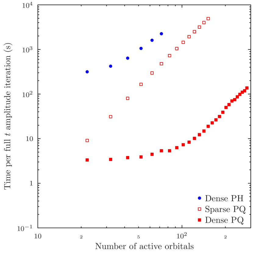
Figure 2: Scaling of the new dense tensor implementations of PQ and PH compared to the earlier implementations(Parkhill and Head-Gordon, 2010c) based on sparse tensors. Note the logarithmic scale.

Molecule	$n_{\text{orb}}$	SCF		PP		B matrix		PQ ints		PQ t		PQ perm		PQ flop		PH ints		PH t		PH perm		PH flop
C4H6	22	0.	23	0.	35	0.	68	0.	00	66.	63	1.	3	1.	8	0.	05	6942.	94	4.	8	14.	2
C6H8	32	0.	27	0.	73	0.	86	0.	01	75.	42	1.	8	3.	9	0.	15	12228.	76	8.	8	28.	2
C8H10	42	0.	35	1.	45	1.	13	0.	03	90.	27	2.	7	7.	5	0.	39	20436.	82	12.	8	41.	9
C10H12	52	0.	44	2.	37	1.	65	0.	06	105.	08	4.	3	12.	7	0.	79	39056.	60	16.	8	48.	9
C12H14	62	0.	64	3.	65	2.	47	0.	11	120.	68	5.	6	17.	8	1.	49	59499.	11	19.	2	54.	5
C14H16	72	1.	10	5.	05	3.	89	0.	18	144.	63	7.	1	21.	7	2.	72	83323.	67	20.	4	58.	4
C16H18	82	1.	71	7.	10	5.	89	0.	26	144.	47	9.	2	29.	8
C18H20	92	2.	48	9.	92	8.	83	0.	37	169.	61	11.	9	34.	9
C20H22	102	3.	54	13.	07	13.	56	0.	48	197.	28	13.	7	39.	6
C22H24	112	6.	98	19.	06	18.	81	0.	68	225.	59	15.	5	44.	0
C24H26	122	7.	83	24.	13	26.	78	0.	89	274.	37	18.	5	47.	5
C26H28	132	9.	11	30.	51	37.	99	1.	11	332.	18	20.	6	50.	0
C28H30	142	10.	53	37.	52	55.	58	1.	40	400.	48	22.	5	52.	8
C30H32	152	12.	07	46.	01	70.	23	1.	73	510.	74	26.	5	51.	5
C32H34	162	13.	64	55.	16	104.	76	2.	11	610.	46	27.	1	53.	4
C34H36	172	15.	62	66.	35	130.	54	2.	51	713.	33	27.	6	54.	9
C36H38	182	17.	26	77.	59	161.	94	2.	99	847.	72	28.	5	56.	1
C38H40	192	19.	32	94.	63	242.	02	3.	50	1055.	37	31.	7	55.	3
C40H42	202	21.	33	107.	16	339.	07	4.	14	1351.	42	30.	8	51.	7
C42H44	212	25.	34	125.	60	436.	98	4.	77	1566.	79	32.	0	51.	7
C44H46	222	27.	52	143.	47	586.	43	5.	48	1888.	20	32.	5	51.	4
C46H48	232	30.	12	166.	73	1108.	01	6.	28	2020.	66	32.	0	51.	7
C48H50	242	33.	16	188.	38	1366.	80	7.	31	2343.	37	32.	4	51.	6

Table 3: Comparison of wall timings in seconds for the computational procedure of PQ and PH as a function of active orbitals $n_{\text{orb}}$. The third through sixth columm detail the base procedure: SCF solution followed by the PP orbital optimization and the formation of the RI B matrix, while columns 6, 7, 8 and 9 (10, 11, 12 and 13) give the time needed to compute the integrals for PQ (PH), the total time for the $t$ amplitude iterations needed to solve PQ (PH), as well as the fraction of total runtime in percent spent in permutation operations and floating point compute kernels, respectively.

Time spent in multiplication kernels (5)	3617.	84
Time spent in addition kernels	42.	34
Time spent in permutations	2331.	36
Memory allocation	761.	73
Integrals	9.	27
Diagonal zeroing	39.	72
Denominator application	0.	17
Sum of above	6802.	40
Total elapsed wall time	7047.	52

Table 4: Distribution of computational effort in the solution of the PQ model for C52H54. The timings include all steps in solving the PQ model: the solution of the $t$ and $\lambda$ amplitudes as well as the formation of the one- and two-particle density matrices $\gamma$ and $\Gamma$, respectively.

Kernel	Time (s)		Scaling	BLAS
$o(x)\leftarrow l(x)r(x)$	0.	00	$N$	no
$o(x,y)\leftarrow l(x,y)r(x,y)$	0.	01	$N^{2}$	no
$o(x)\leftarrow l(x)r(x)$	0.	05	$N$	no
$o(x,y)\leftarrow l(x)r(y)$	0.	07	$N^{2}$	no
$o(x)\leftarrow\sum_{y}l(x,y)r(y)$	0.	56	$N^{2}$	yes
$o(x,y,z)\leftarrow l(y,z)r(x)$	1.	27	$N^{3}$	no
$o(x,y)\leftarrow l(x,y)r(y)$	13.	51	$N^{2}$	no
$o(x)\leftarrow\sum_{y}l(x,y)r(x,y)$	21.	25	$N^{2}$	yes
$o(x,y)\leftarrow l(x,y)r(x)$	23.	31	$N^{2}$	no
$o(x,y)\leftarrow\sum_{z}l(x,z)r(y,z)$	24.	90	$N^{3}$	yes
$o(x,y,z)\leftarrow l(x,y,z)r(z)$	28.	69	$N^{3}$	no
$o(x,y)\leftarrow l(x,y)r(x,y)$	47.	89	$N^{2}$	no
$o(x,y,z)\leftarrow\sum_{w}l(y,z,w)r(x,w)$	83.	04	$N^{4}$	yes
$o(x,y,z)\leftarrow l(x,z)r(y,z)$	110.	31	$N^{3}$	no
$o(x,y,z)\leftarrow l(x,y,z)r(x)$	125.	27	$N^{3}$	no
$o(x,y,z)\leftarrow\sum_{w}l(x,y,w)r(z,w)$	127.	99	$N^{4}$	yes
$o(x,y,z)\leftarrow l(x,y,z)r(x,z)$	145.	91	$N^{3}$	no
$o(x,y,z)\leftarrow l(x,y,z)r(x,y)$	151.	28	$N^{3}$	no
$o(x,y,z)\leftarrow l(x,y)r(y,z)$	501.	45	$N^{3}$	no
$o(x,y,z)\leftarrow l(x,y)r(x,z)$	502.	06	$N^{3}$	no
$o(x,y)\leftarrow\sum_{z}l(x,y,z)r(y,z)$	521.	73	$N^{3}$	yes
$o(x,y)\leftarrow\sum_{z}l(x,y,z)r(x,z)$	1187.	29	$N^{3}$	yes

Table 5: Multiplication kernels that appear in the three-pair intermediates PQ model with timings for the C52H54 molecule.

IV.2 Accuracy

To study the accuracy of the generated models in the perfect pairing hierarchy, in the following we apply the PP, PQ, and PH models on the $\pi$ space of the polyenes used above for the scaling study, the symmetric and asymmetric dissociation of the H50 chain, as well as the strongly correlated $\pi$ space of polyacene molecules. Hydrogen chains and polyacenes are standard chemical models for testing models of strong correlation(Tsuchimochi and Scuseria, 2009; Sinitskiy et al., 2010; Phillips and Zgid, 2014). The $\pi$ space correlation energies for the polyenes are shown in 6, from which the accuracy of the PP hierarchy already becomes apparent: even for the largest system PH captures 99.3% of the full correlation energy.

Molecule	PP	PQ	PH	DMRG
C4H6	-0.080460	-0.091502	-0.091502	-0.091502
C8H10	-0.143334	-0.172876	-0.176908	-0.177127
C12H14	-0.205042	-0.253097	-0.261466	-0.262297
C16H18	-0.266492	-0.333088	-0.345899	-0.347403
C20H22	-0.327882	-0.413030	-0.430310	-0.432498
C24H26	-0.389257	-0.492961	-0.514717	-0.517591
C28H30	-0.450629	-0.572889	-0.599123	-0.602684
C32H34	-0.512000	-0.652816	-0.683528	-0.687777
C36H38	-0.573371	-0.732743	-0.767934	-0.772870
C40H42	-0.634742	-0.812669	-0.852338	-0.857963
C44H46	-0.696112	-0.892595	-0.936743	-0.943056
C48H50	-0.757483	-0.972521	-1.021147	-1.028149

Table 6: Polyene $\pi$ space correlation energy in the STO-3G basis set with generalized Pipek–Mezey localized occupied orbitals paired with Sano virtuals with the PP, PQ, and PH models, compared to DMRG values from reference 26. The size of the active space coincides with the number of C atoms in the molecule. Note that PQ and PH are exact for the (4e,4o) system in C4H6.

Next, while H50 is chemically uninteresting, it is an excellent system for studying models for strong correlation. When the interatomic separation is increased, the system switches from a metallic state to an insulating state with strong multireference character in the intermediate region that isn’t captured by CC with full single and double (CCSD) or CC with full single and double and perturbative triple excitations (CCSD(T))(Hachmann et al., 2006). In the symmetric dissociation, the equispaced chain is stretched apart into noninteracting H atoms. In the asymmetric dissociation, the system is composed of 25 H2 molecules with bond length $R=1.4a_{0}$, where $a_{0}$ is the Bohr radius, that are placed on the $z$ axis, and the energy is studied as a function of the intermolecular distance. Here, the STO-6G basis set(Hehre et al., 1969) and PP optimized orbitals are used. The two-electron integrals for PQ and PH are generated with CD using the threshold $\Delta_{\text{Cholesky}}=10^{-8}$. The DMRG data has been taken from reference 26.

The obtained total energies for asymmetric dissociation are shown in 3. For large intermolecular separation, the system is essentially composed of noninteracting H2 molecules, for which already PP is exact. When the molecules are pushed closer, the differences in the performance of the models become apparent: while PP quickly starts deviating from the exact solution, PQ and PH stay more accurate on a wider range of correlation strength. This is also clearly visible in the fraction of correlation energy captured by the models shown in 4. For the most strongly correlated geometry, in which the atoms are equidistant, PP, PQ, and PH capture 35.2%, 63.9% and 87.9% of the correlation energy, respectively. PH becomes practically exact (disagreeing from the DMRG correlation energy by at most 1%) at the distance $d=2.0a_{0}$, where it captures 99.2% of the correlation energy. For PQ, practical exactness is reached at $d=2.8a_{0}$ with 99.4% of the correlation energy retained. PP reaches exactness at $d=4.2a_{0}$, where it describes 99.0% of the correlation.

The symmetric dissociation is a much harder problem, but even here the models fare seemingly well, as shown by the total and correlation energy plots in LABEL:fig:sym,fracsym, respectively. As before with the asymmetric stretch, a clear hierarchy is again seen between the models, with the most strongly correlated geometry showing 22.0%, 47.6%, and 80.9% of the correlation energy being captured by PP, PQ, and PH, respectively. As the chain is pulled apart, the models quickly become more accurate, PH reaching practical exactness at separation $d=2.8a_{0}$ where it captures 99.0% of the correlation energy. Unfortunately, for larger interatomic spacings the CC iterations diverged for PQ and PH (both with the zero and PP guess for the amplitudes), thus some data points are missing. However, because PP appears to become better and better for large separations, the divergence issue might be solved by the use of a better preconditioner.

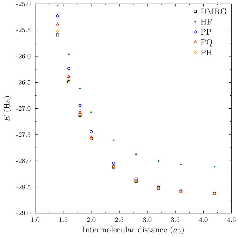
Figure 3: Asymmetric dissociation of the H50 chain into equidistant hydrogen molecules with fixed bond length $R=1.4a_{0}$.

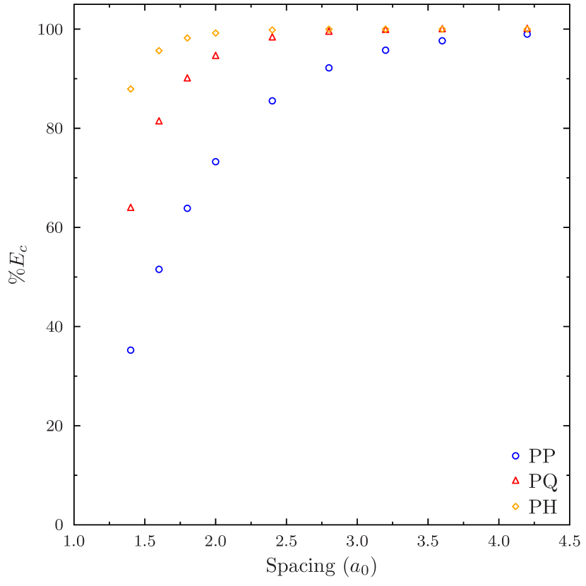
Figure 4: Fraction of correlation energy captured by the PP, PQ, and PH models for the asymmetric dissociation of the H50 chain.

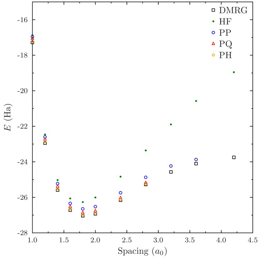
Figure 5: Symmetric dissociation of the H50 chain into equidistant hydrogen atoms.

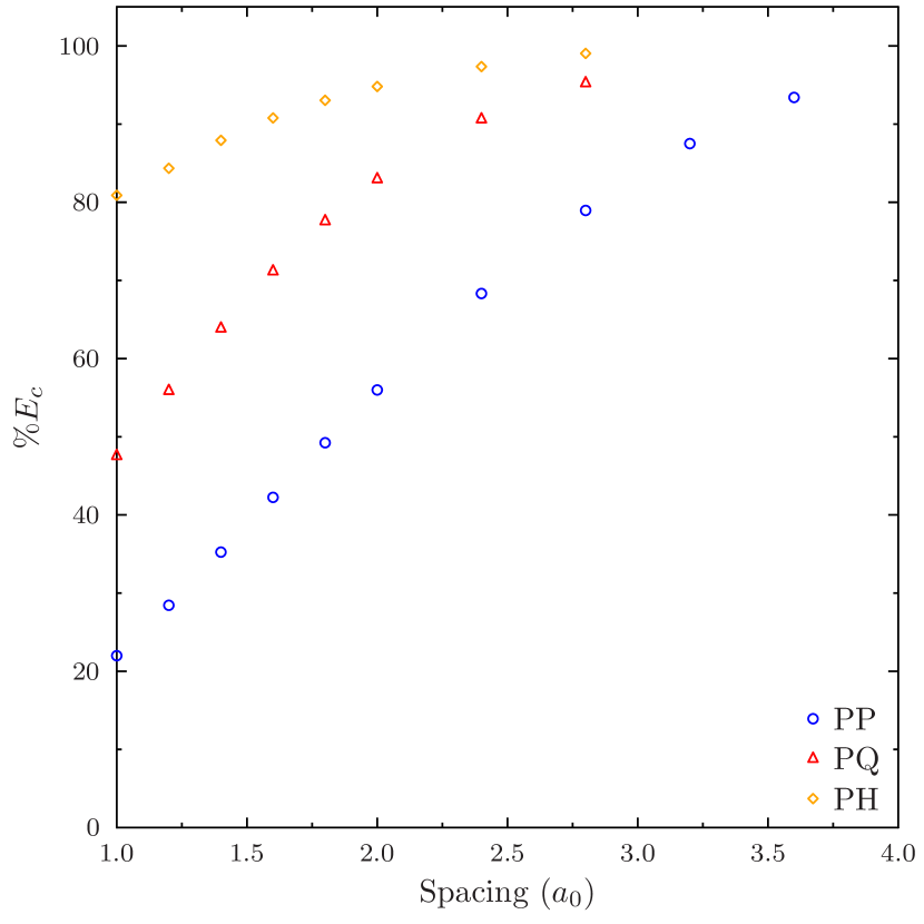
Figure 6: Fraction of correlation energy captured by the PP, PQ, and PH models for the symmetric dissociation of the H50 chain.

The linear polyacenes are known to exhibit multiradical behavior in the $\pi$ space(Hachmann et al., 2007). Next, we will try to match the DMRG energies in the STO-3G basis from reference 69 using their geometries. Generalized Pipek–Mezey localized active occupied orbitals paired with Sano virtuals were used. The energies obtained with the PP, PQ, and PH models compared against the DMRG reference are shown in 7. Here, the models capture 44%–59%, 69%–88%, and 96%–99% of the DMRG correlation energy for PP, PQ, and PH, respectively. We can also compare the natural occupation numbers produced by PP, PQ, and PH against the ones from DMRG; this is done in 7. While PP and PQ succesfully capture a significant amount of the correlation energy, they fail to capture the strong correlation effects in the $\pi$ space of the polyacenes. For PP, the occupation number plot has an almost step function like character, while PQ reproduces some curvature but is still far from the DMRG reference. In contrast, PH reproduces a clear signal of strong correlation that is strikingly similar to the DMRG reference values. Quantitative agreement with DMRG is not, however, reached, which we primarily attribute to the use of non-optimal orbitals. Indeed, other choices for the orbital localization method (see the Supplementary Material) demonstrate that a different choice for the active space orbitals affects the natural orbital occupation numbers, as well as the fraction of energy captured. Furthermore, as Pipek–Mezey localized Hartree–Fock orbitals were found to yield better energies than PP optimized orbitals at the UPH level of theory, we conclude that as has been seen for CCVB(Small et al., 2014), PQ and PH presumably need orbitals that are less localized than those reproduced by PP, and the best choice for the (non-optimized) orbitals is still an open question.

Molecule	Active space	PP	PQ	PH	DMRG
2acene	(10e,10o)	-0.104902	-0.157684	-0.177098	-0.178294
3acene	(14e,14o)	-0.144544	-0.213115	-0.249895	-0.254307
4acene	(18e,18o)	-0.190182	-0.279345	-0.325491	-0.332661
5acene	(22e,22o)	-0.228839	-0.335088	-0.401098	-0.412627
6acene	(26e,26o)	-0.265084	-0.393537	-0.479533	-0.495683
8acene	(34e,34o)	-0.322287	-0.495219	-0.641147	-0.668526
10acene	(42e,42o)	-0.382622	-0.595840	-0.803505	-0.838580
12acene	(50e,50o)	-0.444834	-0.698165	-0.968521	-1.007378a

Table 7: Polyacene $\pi$ space correlation energy in the STO-3G basis set with generalized Pipek–Mezey localized occupied orbitals paired with Sano virtuals with the PP, PQ, and PH models, compared to DMRG values from reference 69. Note that PQ and PH are exact for the (4e,4o) system in C4H6. ^aDMRG value of reference 69 was not converged.

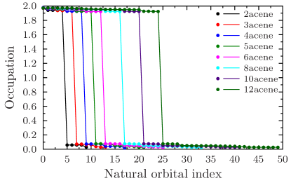
(a) PP

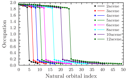
(b) PQ

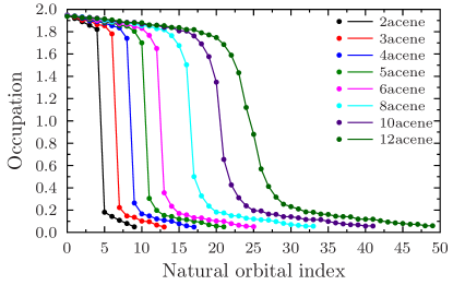
(c) PH

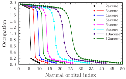
(d) DMRG data from reference 69

Figure 7: Polyacene $\pi$ space natural orbital occupation numbers.

V Summary and Discussion

We have described the low-scaling dense tensor implementation of a family of truncated CC methods, and generated efficient implementations of the PQ and PH models. High-rank tensors are expressed in terms of a considerable number of subtensors, and summations over Kronecker delta indices are performed before computer code is generated. As straightforward truncations of CC theory, the models inherit all the properties of the parent theory, such as size extensivity, and pre-existing machinery for the calculation of properties could be used.

We have demonstrated impressive speedups (of roughly 200-500 times) compared to the earlier implementation that already had the correct $O(N^{4})$ scaling for PQ, and demonstrated the rapid convergence of the PP, PQ, and PH models in describing strong correlation with applications to the dissociation of the H50 chain. Although only minimal basis sets have been used in the present work due to limited availability of high-level reference data, the runtime of the models after integral transformation is basis set independent due to the use of an active space (and the lack of orbital optimization that has not been pursued in the present work). While the models are already computationally fast enough to allow their use in studies of chemical problems, we believe they can still be made even faster by a variety of approaches. Most importantly, the role of the intermediates in the paired theories are clearly different from the intermediates in full-rank CC theory. A thorough procedure for identifying common factors between different contributions, as well as a graph-type approach for determining the optimal set of intermediates, could plausibly yield a further order of magnitude speedup to the existing implementation. In the case of closed-shell molecules, spin summation of the model would reduce storage costs for the amplitudes by roughly 50%, and cut down on computational costs as well. A reorganization of the way the amplitude updates are performed might yield convergence in a smaller number of iterations(Matthews and Stanton, 2015). Because of the mathematical structure of the models, the storage of the tensors is already distributed, and massively parallel implementations of the models could be pursued.

While we have demonstrated that the truncation hierarchy advocated in the present work allows for applications to large systems, it is further important to note that in systems with little static correlation it is possible to further speed things up. While in PQ and PH the excitation amplitude tensors have similar storage requirements (within an order of magnitude) as shown in 2, the runtime tends to be dominated by the highest excitations due to the larger amount of antisymmetrizations necessary in the CC diagrams. Thus, should the higher excitation operators turn out to be insignificant, disabling them can yield further speedups. For example, the PH model with only single and double (and triple and quadruple) excitations enabled is essentially a local CCSD (CCSDTQ) approach, if the treatment is based on localized orbitals.

As we have seen in the application to the acene series, the choice of orbitals may be important for the perfect pairing hierarchy of models, which we will address in future work. In addition, we wish to extend the PQ and PH models to open-shell systems, as well as to include the description of dynamic correlation. The similarities between the PP truncation hierarchy and local CC methods could also be further explored.

Supplementary Material

See supplementary material for results on the polyacenes with various choices for the active space orbitals.

References

- Hohenberg and Kohn (1964) P. Hohenberg and W. Kohn, Phys. Rev. 136, B864 (1964).
- Kohn and Sham (1965) W. Kohn and L. J. Sham, Phys. Rev. 140, A1133 (1965).
- Kurzweil et al. (2009) Y. Kurzweil, K. V. Lawler, and M. Head-Gordon, Mol. Phys. 107, 2103 (2009).
- Thomas et al. (2015) R. E. Thomas, Q. Sun, A. Alavi, and G. H. Booth, J. Chem. Theory Comput. 11, 5316 (2015), arXiv:1510.03635 .
- Manni et al. (2016) G. L. Manni, S. D. Smart, and A. Alavi, J. Chem. Theory Comput. 12, 1245 (2016).
- Schriber and Evangelista (2016) J. B. Schriber and F. A. Evangelista, J. Chem. Phys. 144, 161106 (2016), arXiv:1603.08063 .
- Tubman et al. (2016) N. M. Tubman, J. Lee, T. Y. Takeshita, M. Head-Gordon, and K. B. Whaley, J. Chem. Phys. 145, 044112 (2016), arXiv:1603.02686 .
- Liu and Hoffmann (2016) W. Liu and M. R. Hoffmann, J. Chem. Theory Comput. 12, 1169 (2016).
- Zhang and Evangelista (2016) T. Zhang and F. A. Evangelista, J. Chem. Theory Comput. , acs.jctc.6b00639 (2016).
- Holmes et al. (2016) A. A. Holmes, N. M. Tubman, and C. J. Umrigar, J. Chem. Theory Comput. , acs.jctc.6b00407 (2016).
- Čížek (1966) J. Čížek, J. Chem. Phys. 45, 4256 (1966).
- Lyakh et al. (2012) D. I. Lyakh, M. Musiał, V. F. Lotrich, and R. J. Bartlett, Chem. Rev. 112, 182 (2012).
- Krylov et al. (1998) A. I. Krylov, C. D. Sherrill, E. F. C. Byrd, and M. Head-Gordon, J. Chem. Phys. 109, 10669 (1998).
- Parkhill et al. (2009) J. A. Parkhill, K. Lawler, and M. Head-Gordon, J. Chem. Phys. 130, 084101 (2009).
- Parkhill and Head-Gordon (2010a) J. A. Parkhill and M. Head-Gordon, J. Chem. Phys. 133, 024103 (2010a).
- Hurley et al. (1953) A. C. Hurley, J. Lennard-Jones, and J. A. Pople, Proc. R. Soc. A Math. Phys. Eng. Sci. 220, 446 (1953).
- Hunt et al. (1972) W. J. Hunt, P. J. Hay, and W. A. Goddard III, J. Chem. Phys. 57, 738 (1972).
- Ukrainskii (1977) I. I. Ukrainskii, Theor. Math. Phys. 32, 816 (1977).
- Goddard and Harding (1978) W. A. Goddard and L. B. Harding, Annu. Rev. Phys. Chem. 29, 363 (1978).
- Cullen (1996) J. Cullen, Chem. Phys. 202, 217 (1996).
- White (1992) S. R. White, Phys. Rev. Lett. 69, 2863 (1992).
- Chan et al. (2008) G. K.-L. Chan, J. J. Dorando, D. Ghosh, J. Hachmann, E. Neuscamman, H. Wang, and T. Yanai, in Front. Quantum Syst. Chem. Phys., Vol. 18 (Springer Netherlands, Dordrecht, 2008) pp. 49–65, arXiv:arXiv:0711.1398v1 .
- Marti and Reiher (2010) K. H. Marti and M. Reiher, Zeitschrift für Phys. Chemie 224, 583 (2010).
- Wouters and Van Neck (2014) S. Wouters and D. Van Neck, Eur. Phys. J. D 68, 272 (2014), arXiv:1407.2040 .
- Olivares-Amaya et al. (2015) R. Olivares-Amaya, W. Hu, N. Nakatani, S. Sharma, J. Yang, and G. K.-L. Chan, J. Chem. Phys. 142, 034102 (2015).
- Hachmann et al. (2006) J. Hachmann, W. Cardoen, and G. K.-L. Chan, J. Chem. Phys. 125, 144101 (2006), arXiv:0606115 [cond-mat] .
- Small and Head-Gordon (2009) D. W. Small and M. Head-Gordon, J. Chem. Phys. 130, 084103 (2009).
- Small and Head-Gordon (2011) D. W. Small and M. Head-Gordon, Phys. Chem. Chem. Phys. 13, 19285 (2011).
- Small et al. (2014) D. W. Small, K. V. Lawler, and M. Head-Gordon, J. Chem. Theory Comput. 10, 2027 (2014).
- Arponen (1983) J. Arponen, Ann. Phys. (N. Y). 151, 311 (1983).
- Arponen et al. (1987a) J. S. Arponen, R. F. Bishop, and E. Pajanne, Phys. Rev. A 36, 2519 (1987a).
- Arponen et al. (1987b) J. S. Arponen, R. F. Bishop, and E. Pajanne, Phys. Rev. A 36, 2539 (1987b).
- Shepard et al. (2014a) R. Shepard, G. Gidofalvi, and S. R. Brozell, J. Chem. Phys. 141, 064105 (2014a).
- Shepard et al. (2014b) R. Shepard, G. Gidofalvi, and S. R. Brozell, J. Chem. Phys. 141, 064106 (2014b).
- Parkhill and Head-Gordon (2010b) J. A. Parkhill and M. Head-Gordon, J. Chem. Phys. 133, 124102 (2010b).
- Parkhill et al. (2011) J. A. Parkhill, J. Azar, and M. Head-Gordon, J. Chem. Phys. 134, 154112 (2011).
- Pulay and Hamilton (1988) P. Pulay and T. P. Hamilton, J. Chem. Phys. 88, 4926 (1988).
- Bofill and Pulay (1989) J. M. Bofill and P. Pulay, J. Chem. Phys. 90, 3637 (1989).
- Keller et al. (2015) S. Keller, K. Boguslawski, T. Janowski, M. Reiher, and P. Pulay, J. Chem. Phys. 142, 244104 (2015).
- Parkhill and Head-Gordon (2010c) J. A. Parkhill and M. Head-Gordon, Mol. Phys. 108, 513 (2010c).
- Crawford and Schaefer (2000) T. D. Crawford and H. F. Schaefer, in Rev. Comput. Chem., Vol. 14, edited by K. B. Lipkowitz and D. B. Boyd (Wiley-VCH, John Wiley and Sons, Inc., New York, 2000) pp. 33–136.
- Bartlett and Musiał (2007) R. Bartlett and M. Musiał, Rev. Mod. Phys. 79, 291 (2007).
- De Lathauwer (2008a) L. De Lathauwer, SIAM J. Matrix Anal. Appl. 30, 1033 (2008a).
- De Lathauwer (2008b) L. De Lathauwer, SIAM J. Matrix Anal. Appl. 30, 1022 (2008b).
- Beran et al. (2005) G. J. O. Beran, B. Austin, A. Sodt, and M. Head-Gordon, J. Phys. Chem. A 109, 9183 (2005).
- Van Voorhis and Head-Gordon (2000) T. Van Voorhis and M. Head-Gordon, Chem. Phys. Lett. 317, 575 (2000).
- Pulay (1983) P. Pulay, Chem. Phys. Lett. 100, 151 (1983).
- Saebo and Pulay (1993) S. Saebo and P. Pulay, Annu. Rev. Phys. Chem. 44, 213 (1993).
- Foster and Boys (1960) J. Foster and S. Boys, Rev. Mod. Phys. 32, 300 (1960).
- Edmiston and Ruedenberg (1963) C. Edmiston and K. Ruedenberg, Rev. Mod. Phys. 35, 457 (1963).
- Pipek and Mezey (1989) J. Pipek and P. G. Mezey, J. Chem. Phys. 90, 4916 (1989).
- Lehtola and Jónsson (2014) S. Lehtola and H. Jónsson, J. Chem. Theory Comput. 10, 642 (2014).
- Sano (2000) T. Sano, J. Mol. Struct. THEOCHEM 528, 177 (2000).
- Pulay (1980) P. Pulay, Chem. Phys. Lett. 73, 393 (1980).
- Scuseria et al. (1986) G. E. Scuseria, T. J. Lee, and H. F. Schaefer, Chem. Phys. Lett. 130, 236 (1986).
- Vahtras et al. (1993) O. Vahtras, J. Almlöf, and M. Feyereisen, Chem. Phys. Lett. 213, 514 (1993).
- Beebe and Linderberg (1977) N. H. F. Beebe and J. Linderberg, Int. J. Quant. Chem. 12, 683 (1977).
- Epifanovsky et al. (2013) E. Epifanovsky, D. Zuev, X. Feng, K. Khistyaev, Y. Shao, and A. I. Krylov, J. Chem. Phys. 139, 134105 (2013).
- Shao et al. (2014) Y. Shao, Z. Gan, E. Epifanovsky, a. T. B. Gilbert, M. Wormit, J. Kussmann, a. W. Lange, A. Behn, J. Deng, X. Feng, D. Ghosh, M. Goldey, P. R. Horn, L. D. Jacobson, I. Kaliman, R. Z. Khaliullin, T. Kus, A. Landau, J. Liu, E. I. Proynov, Y. M. Rhee, R. M. Richard, M. a. Rohrdanz, R. P. Steele, E. J. Sundstrom, H. L. W. III, P. M. Zimmerman, B. A. D. Zuev, E. Alguire, B. Austin, G. J. O. Beran, Y. a. Bernard, E. Berquist, K. Brandhorst, K. B. Bravaya, S. T. Brown, D. Casanova, C.-M. Chang, Y. Chen, S. H. Chien, K. D. Closser, D. L. Crittenden, M. Diedenhofen, R. a. D. Jr., H. Do, a. D. Dutoi, R. G. Edgar, S. Fatehi, L. Fusti-Molnar, A. Ghysels, A. Golubeva-Zadorozhnaya, J. Gomes, M. W. D. Hanson-Heine, P. H. P. Harbach, a. W. Hauser, E. G. Hohenstein, Z. C. Holden, T.-C. Jagau, B. K. H. Ji, K. Khistyaev, J. Kim, R. a. King, P. Klunzinger, D. Kosenkov, T. Kowalczyk, C. M. Krauter, K. U. Lao, A. Laurent, K. V. Lawler, S. V. Levchenko, C. Y. Lin, F. Liu, E. Livshits, R. C. Lochan, A. Luenser, P. Manohar, S. F. Manzer, S.-P. Mao, N. Mardirossian, a. V. Marenich, S. a. Maurer, N. J. Mayhall, C. M. Oana, R. Olivares-Amaya, D. P. O’Neill, J. a. Parkhill, T. M. Perrine, R. Peverati, A. Prociuk, D. R. Rehn, E. Rosta, N. J. Russ, S. M. Sharada, S. Sharma, D. W. Small, A. Sodt, T. Stein, D. Stück, Y.-C. Su, a. J. W. Thom, T. Tsuchimochi, V. Vanovschi, L. Vogt, O. Vydrov, T. Wang, M. a. Watson, J. Wenzel, A. White, C. F. Williams, S. Yeganeh, S. R. Yost, Z.-Q. You, I. Y. Zhang, X. Zhang, Y. Zhao, B. R. Brooks, G. K. L. Chan, D. M. Chipman, C. J. Cramer, W. A. G. III, M. S. Gordon, W. J. Hehre, A. Klamt, H. F. S. III, M. W. Schmidt, C. D. Sherrill, D. G. Truhlar, A. Warshel, X. Xuaf, A. Aspuru-Guzik, R. Baer, a. T. Bell, N. a. Besley, J.-D. Chai, A. Dreuw, B. D. Dunietz, T. R. Furlani, S. R. Gwaltney, C.-P. Hsu, Y. Jung, J. Kong, D. S. Lambrecht, W. Liang, C. Ochsenfeld, V. a. Rassolov, L. V. Slipchenko, J. E. Subotnik, T. V. Voorhis, J. M. Herbert, a. I. Krylov, P. M. W. Gill, and M. Head-Gordon, Mol. Phys. , 37 (2014).
- Lehtola et al. (2012) J. Lehtola, M. Hakala, A. Sakko, and K. Hämäläinen, J. Comput. Chem. 33, 1572 (2012).
- Lehtola (2016) S. Lehtola, “ERKALE - HF/DFT from Hel,” (2016).
- Knizia (2013) G. Knizia, J. Chem. Theory Comput. 9, 4834 (2013).
- Lehtola and Jónsson (2013) S. Lehtola and H. Jónsson, J. Chem. Theory Comput. 9, 5365 (2013).
- Hehre et al. (1969) W. J. Hehre, R. F. Stewart, and J. A. Pople, J. Chem. Phys. 51, 2657 (1969).
- Weigend et al. (2002) F. Weigend, A. Köhn, and C. Hättig, J. Chem. Phys. 116, 3175 (2002).
- Tsuchimochi and Scuseria (2009) T. Tsuchimochi and G. E. Scuseria, J. Chem. Phys. 131, 121102 (2009).
- Sinitskiy et al. (2010) A. V. Sinitskiy, L. Greenman, and D. A. Mazziotti, J. Chem. Phys. 133, 014104 (2010).
- Phillips and Zgid (2014) J. J. Phillips and D. Zgid, J. Chem. Phys. 140, 241101 (2014).
- Hachmann et al. (2007) J. Hachmann, J. J. Dorando, M. Avilés, and G. K.-L. Chan, J. Chem. Phys. 127, 134309 (2007).
- Matthews and Stanton (2015) D. A. Matthews and J. F. Stanton, J. Chem. Phys. 143, 204103 (2015).