Baryonic acoustic oscillations from 21cm intensity mapping: the Square Kilometre Array case

Abstract

We quantitatively investigate the possibility of detecting baryonic acoustic oscillations (BAO) using single-dish 21cm intensity mapping observations in the post-reionization era. We show that the telescope beam smears out the isotropic BAO signature and, in the case of the Square Kilometer Array (SKA) instrument, makes it undetectable at redshifts $z\gtrsim 1$. We however demonstrate that the BAO peak can still be detected in the radial 21cm power spectrum and describe a method to make this type of measurements. By means of numerical simulations, containing the 21cm cosmological signal as well as the most relevant Galactic and extra-Galactic foregrounds and basic instrumental effect, we quantify the precision with which the radial BAO scale can be measured in the 21cm power spectrum.

We systematically investigate the signal-to-noise and the precision of the recovered BAO signal as a function of cosmic variance, instrumental noise, angular resolution and foreground contamination. We find that the expected noise levels of SKA would degrade the final BAO errors by $\sim 5\%$ with respect to the cosmic-variance limited case at low redshifts, but that the effect grows up to $\sim 65\%$ at $z\sim 2-3$. Furthermore, we find that the radial BAO signature is robust against foreground systematics, and that the main effect is an increase of $\sim 20\%$ in the final uncertainty on the standard ruler caused by the contribution of foreground residuals as well as the reduction in sky area needed to avoid high-foreground regions. We also find that it should be possible to detect the radial BAO signature with high significance in the full redshift range.

We conclude that a 21cm experiment carried out by the SKA should be able to make direct measurements of the expansion rate $H(z)$ with measure the expansion with competitive per-cent level precision on redshifts $z\lesssim 2.5$.

1 Introduction

The spatial distribution of matter in the Universe is sensitive to the value of the cosmological parameters. Constraints on those can thus be placed by comparing the statistical properties of the density field against predictions from theoretical models. Unfortunately, the true matter density is not directly observable, and therefore one must resort to using proxies of it, such as the number density of galaxies or line emission intensity of cosmic neutral hydrogen (HI).

A promising and new way of tracing the large-scale structure of the Universe is to carry out low angular resolution radio observations to detect the 21cm radiation from cosmic neutral hydrogen in the post-reionization epoch. The idea is not to detect individual galaxies through their 21cm emission, but rather to measure the combined flux in wide patches of the sky containing many galaxies. This technique is called intensity mapping (Bharadwaj et al., 2001; Bharadwaj & Sethi, 2001; Battye et al., 2004; McQuinn et al., 2006; Chang et al., 2008; Loeb & Wyithe, 2008; Villaescusa-Navarro et al., 2014; Bull et al., 2015a). Under the assumption that the measured 21cm flux traces the perturbations in the matter density on large-scales, we can use the clustering properties of the cosmic HI, as observed from 21cm intensity mapping surveys, to put constraints on the value of the cosmological parameters (Bull et al., 2015a; Villaescusa-Navarro et al., 2015; Carucci et al., 2015).

Baryonic acoustic oscillations (BAO), originated in the early Universe by the competition between the gravitational interaction and the radiation pressure of photons tightly coupled to baryons, leave an imprint in the late-time matter density in the form of a statistically preferred separation between density peaks of $r_{s}\sim 110~{}h^{-1}{\rm Mpc}$, corresponding to the size of the sound horizon at the time of the baryon-photon decoupling. This translates into a distinct peak in the matter/galaxy two-point correlation function, or as a set of wiggles in the matter/galaxy power spectrum on scales $k\sim[0.05-0.3]~{}h{\rm Mpc}^{-1}$ with frequency $r_{s}$. The BAO signature thus constitutes a cosmological standard ruler, whose size depends on well understood physics of the early Universe. By measuring them in the temperature anisotropies of the cosmic microwave background (CMB) and in the clustering pattern of matter tracers, it is possible to measure the value of the Hubble rate and the angular diameter distance as a function of redshift.

The main advantage of the BAO signal resides in its robustness against systematic effects: it is difficult for non-cosmological effects to mimic or shift the position of the BAO feature in the correlation function or power spectrum. Furthermore, given the large-scale nature of the BAO signal, the effects induced by the non-linear gravitational evolution are well captured by perturbation theory (e.g. Crocce & Scoccimarro, 2008; Padmanabhan & White, 2009; Baldauf et al., 2015; Peloso et al., 2015).

The BAO scale has been measured in the 2pt/3pt statistics of galaxy surveys (see e.g. Cole et al., 2005; Eisenstein et al., 2005; Anderson et al., 2014; Gil-Marín et al., 2016; Beutler et al., 2016; Alam et al., 2016; Slepian et al., 2016), in the Ly$\alpha$-forest (Delubac et al., 2015), in the distribution of galaxy clusters (Veropalumbo et al., 2016) and in the spatial distribution of voids (Kitaura et al., 2016). Upcoming and future radio experiments such as the Canadian Hydrogen Intensity Mapping Experiment (CHIME), the Ooty Radio Telescope (ORT), BINGO Battye et al. (2012) and the Square Kilometre Array (SKA) will survey large areas of the sky using the intensity mapping technique in the post-reionization era. In this paper we investigate the prospects of detecting the BAO from 21cm intensity mapping observations, focusing on the SKA1-MID instrument.

An ideal intensity mapping experiment would cover the largest possible field of view with as large angular resolution as possible. Since the angular scales probed by a radio interferometer are $\lambda/b_{\rm max}\lesssim\theta\lesssim\lambda/b_{\rm min}$, where $b_{\rm max/min}$ are the largest/smallest separation between two antenna elements, these two requirements can only be simultaneously met by building large interferometric arrays of tightly packed receivers. An alternative strategy would be to cover the desired sky footprint with single-dish observations, in which case the angular resolution has a lower bound $\theta\gtrsim\lambda/D_{\rm dish}$ determined by the dish diameter (see Bull et al., 2015b, for a detailed discussion). In this paper we will focus on the latter case, the likely strategy of choice for the SKA1-MID instrument, described in Braun et al. (2015).

We demonstrate that the poor angular resolution inherent to single-dish 21cm observations smears out the BAO peak in the isotropic correlation function or power spectrum, and that in this case cosmological constraints would be driven by the overall shape of the 21cm power spectrum, which is more sensitive to systematic effects. We will however show that the BAO wiggles can be detected in the radial 21cm power spectrum, and thus can be used to make a direct measurement of the expansion rate $H(z)$. In our analysis we will focus on the impact of instrumental effects, such as the system noise, and the presence of Galactic and extra-Galactic foregrounds on our the results.

This paper is organized as follows. In Section 2 we study the impact of the instrumental beam on the detectability of the isotropic BAO peak in single-dish experiments. In Section 3 we describe the simulations and analysis methods used in this work. The results obtained from this analysis and their interpretation are presented in Section 4, where we systematically investigate the impact of each complication (system noise and foregrounds) on the final uncertainties. Finally we discuss main conclusions of this paper in Section 5.

2 BAO and beam size

In this section we investigate the impact of the radio-telescope beam, when observations are carried out using the single-dish technique, on the shape and position of the 21cm intensity mapping BAO. We first analyze the possibility of detecting the isotropic BAO and then we discuss the prospect of using the radial power spectrum to measure the BAO signal.

2.1 Isotropic BAO

At linear order the 21cm power spectrum in real-space can be expressed as

$$P_{\rm 21cm}(k,z)=b_{\rm 21cm}^{2}(z)P_{\rm m}(k,z)$$ (1)

where $b_{\rm 21cm}(z)=\bar{T}_{b}(z)b_{\rm HI}(z)$ is the bias of the 21cm signal and $P_{\rm m}(k)$ is the linear matter power spectrum. $b_{\rm HI}(z)$ and $\bar{T}_{b}(z)$ are the is the HI bias and mean brightness temperature at redshift $z$, the latter given by

$$\bar{T}_{b}(z)=190\frac{H_{0}(1+z)^{2}}{H(z)}\Omega_{\rm HI}(z)h~{}~{}{\rm mK}~{}.$$ (2)

The telescope beam, which for simplicity we will model as being Gaussian, induces a smoothing in the transverse direction

$$\delta_{\rm 21cm,obs}(\mn@boldsymbol{k}_{\bot},k_{\|},z)=e^{-k_{\bot}^{2}R^{2}/2}\delta_{\rm 21cm}(\mn@boldsymbol{k}_{\bot},k_{\|},z)$$ (3)

with $\delta_{\rm 21cm,obs}$, $\delta_{\rm 21cm}$ being the observed and cosmological 21cm modes. The beam angular resolution $\theta_{\rm FWHM}$ is related to the transverse smoothing scale as $R=r(z)\,\theta_{\rm FWHM}/(2\sqrt{2\ln 2})$, where $r(z)$ is the comoving angular diameter distance to redshift $z$. Note that given the frequency dependence of the angular beam size, $\theta_{\rm FWHM}$ is implicitly also a function of $z$.

The observed 21cm power spectrum in real-space can thus be written as

$$P_{\rm 21cm,obs}(k,\mu,z)=e^{-k^{2}R^{2}(1-\mu^{2})}P_{\rm 21cm}(k,z)$$ (4)

and the monopole can be obtained by averaging over all modes sharing the value of $k=\sqrt{k_{\bot}^{2}+k_{\|}^{2}}$:

$$P_{\rm 21cm,obs}(k,z) = P_{\rm 21cm}(k,z)\frac{1}{2}\int_{-1}^{1}e^{-k^{2}R^{2}(1-\mu^{2})}d\mu$$ (5)

$$= \frac{{\mathcal{D}}{(kR)}}{kR}P_{\rm 21cm}(k,z)$$ (6)

where ${\mathcal{D}}(x)$ is the Dawson function. In configuration space the observed 21cm correlation function is given by

$$\xi_{\rm 21cm,obs}(r,z)=\frac{b_{\rm 21cm}^{2}}{2\pi^{2}}\int_{0}^{\infty}k^{2}P_{\rm m}(k,z)\frac{\sin(kr)}{kr}\frac{\mathcal{D}(kR)}{kR}dk$$ (7)

Note that so far we have neglected the effect of redshift-space distortions. This is irrelevant for the main conclusions of this section, however their effect was fully taken into account in the simulations and theoretical models used in Sections 3 and 4.

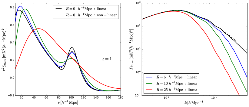
Figure 1: Impact of the telescope beam size on the isotropic BAO shape in configuration (left) and Fourier space (right) at $z=1$. The solid black line shows the results for infinite angular resolution, while the blue, green and red lines represent the observed correlation functions and power spectra for comoving smoothing scales $R=5$, 10 and 25 $h^{-1}$Mpc, respectively. The dashed black line displays the effect of non-linearities, computed using RegPT at 2-loops for ininite angular resolution.

The left panel of Figure 1 shows the observed 21cm correlation function at $z=1$ for the fiducial cosmological model considered in this work (see Section 3.1) for different values of the angular smoothing scale $R$. Following our reference HI model (described in Appendix A), we take $b_{\rm 21cm}=0.231$ mK at $z=1$. As can be seen in the figure, in the idealized case of radio-telescopes having infinite resolution, the BAO peak can easily be detected from single-dish IM observations. On the other hand, as the angular resolution of the telescope decreases (either by going to higher redshift or by decreasing the antenna diameter), the isotropic BAO peak is smeared out by the telescope beam. For angular smoothing scales larger than $\sim 20~{}h^{-1}$Mpc the BAO peak is simply not visible. The Figure also shows, with a dashed black line, the effect of non-linearities on the BAO peak at $z=1$ when the 21cm maps have infinite angular resolution. The effect of non-linearities on the matter power spectrum in real-space was computed using RegPT at 2-loops. As can be seen, even a relatively small angular smoothing like 5 $h^{-1}$Mpc has a larger impact on the BAO signature than effects induced by non-linear gravitational evolution. The right panel of Figure 1 shows the analogous results in Fourier space.

It is useful to quantify the single-dish angular resolution that SKA1-MID will achieve as a function of redshift. MID will consist of an array of 15 m antennae, corresponding to angular resolutions of $\theta_{\rm FWHM}=\lambda/D\simeq 0.8(1+z)$ deg. The corresponding comoving smoothing scale will thus be given by $R=\{11.7,27.2,63.8,104.1\}~{}h^{-1}$Mpc at redshifts $z=\{0.5,1.0,2.0,3.0\}$, respectively. Thus, for redshifts $z\gtrsim 1$ the poor angular resolution of SKA1-MID will prevent the detection the isotropic BAO feature, and cosmological constraints will be driven by the broadband shape of the 21cm power spectrum, which can be significantly affected by systematic effects.

2.2 Radial BAO

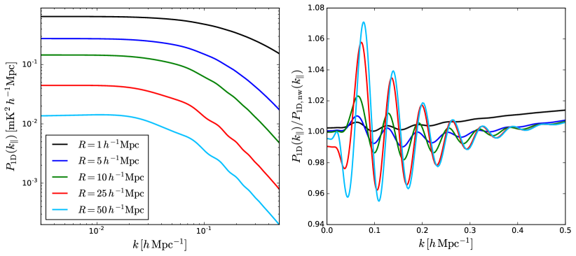
Figure 2: Impact of the telescope beam size on the BAO wiggles of the observed radial power spectrum. The left panel shows the radial power spectra at $z=1$ at linear order for different angular smoothing scales. In the right panel we show the results normalized by the radial 21cm power spectrum for a model with no BAO wiggles.

In what follows we will define the 1D power spectrum $P_{\rm 1D}(k_{\|})$ as

$$\langle\delta_{\rm 1D}(k_{\|},{\bf r}_{\perp})\delta^{*}_{\rm 1D}(k_{\|}^{\prime},{\bf r}_{\perp})\rangle\equiv\delta^{\cal D}(k_{\|}-k_{\|}^{\prime})\,P_{\rm 1D}(k_{\|}),$$ (8)

where $\delta^{\cal D}$ is the Dirac $\delta$-function and $\delta_{\rm 1D}(k_{\|},{\bf r}_{\perp})$ is the one-dimensional Fourier transform along the radial direction of the overdensity field for the transverse coordinate ${\bf r}_{\perp}$. It is straightforward to show that the relation between the 1D and 3D power spectra is given by

$$P_{\rm 1D}(k_{\|},z)=\int\frac{d\mn@boldsymbol{k}_{\bot}}{(2\pi)^{2}}P_{\rm 3D}(k_{\|},\mn@boldsymbol{k}_{\bot},z)~{}.$$ (9)

In the limit of poor angular resolution (i.e. large $R$), it can be shown that

$$\lim\limits_{R\to\infty}\left(\frac{R^{2}}{\pi}e^{-k_{\bot}^{2}R^{2}}\right)=\delta^{\cal D}(\mn@boldsymbol{k_{\bot}})$$ (10)

and therefore we obtain

$$\lim\limits_{R\to\infty}P_{\rm 21cm,obs,1D}(k_{\|},z)=\frac{1}{4\pi R^{2}}P_{\rm 21cm}(k_{\|},z)~{}.$$ (11)

Thus, on the one hand the amplitude of the observed radial 21cm power spectrum scales inversely proportional to the square of the angular smoothing scale. This is simply a consequence of the supression of the contribution from perturbations on small transverse scales caused by the large beam. On the other hand, for sufficiently large angular smoothing scales, the shape of the observed 1D 21cm power spectrum will be the same as that of the 3D power spectrum in the absence of instrumental beam. The consequence of this is that the BAO wiggles can be easily identified in the observed radial 21cm power spectrum for large angular smoothing scales.

These two effects can be seen in Fig. 2, where we show, in the left panel, the observed radial 21cm power spectrum for different angular smoothing scales. As expected, the overall amplitude of the radial power spectrum decreases with increasing angular smoothing scale. On the other hand, the BAO wiggles are more clearly visible when the angular smoothing scale is larger. It is worth noting that the BAO wiggles are not visible in the case where the telescope has a very large angular resolution. The reason for this is that the radial power spectrum at a given wavenumber $k_{\|}$ receives contributions from all transverse scales larger than the smoothing scale. In the limit of zero angular smoothing, the large power on small scales significantly enhances the amplitude the radial power spectrum, effectively decreasing the relative amplitude of the BAO. The right panel of Figure 2 shows the ratio of the 1D power spectrum to the no-BAO power spectrum computed using the Eisenstein & Hu fitting formula (Eisenstein & Hu, 1998) for different angular smoothing scales. As can be seen, the BAO wiggles are present in all cases, but they are more pronounced for large angular smoothing scales. We however emphasize that this effect saturates once the limit of Eq. 11 is achieved. By comparing the red and cyan lines one can see that the relative amplitude of the BAO wiggles barely increases after doubling the angular smoothing scale.

3 Methods

In this section we describe the sky simulations, foreground-cleaning algorithm, radial power spectrum estimation method and the theoretical model we use to evaluate the detectability of the radial BAO scale.

3.1 Simulations

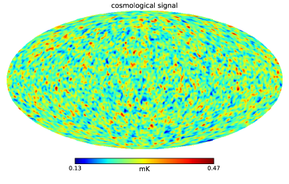
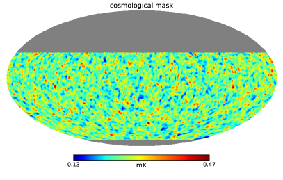
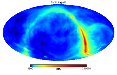
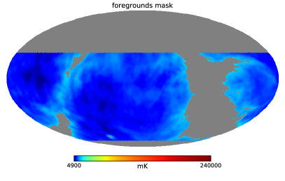
Figure 3: Maps at $\nu=541$ MHz ($z=1.62$) in equatorial coordinates containing the cosmological HI signal and noise only (upper row) and including the contribution from Galactic and extra-Galactic foregrounds, (bottom row). The masks we use in our analysis are shown in the right column. The mask used for simulations without foregrounds is shown in the upper-right panel (the cosmological mask) is defined by a simple cut in declination compatible with SKA the observing site. The bottom-right panel displays the mask we employ for maps containing foregrounds (the foregrounds mask): beyond the declination cuts, we remove regions of high foreground emission.

We used the public code described in Alonso et al. (2014) to generate a suite of 100 simulations of the 21cm intensity mapping signal, as well as the main sources of foreground contamination. We describe here the most important components of these simulations, and refer the reader to Alonso et al. (2014) for further details.

• Cosmological signal. The code uses a simplified lognormal model to relate the cosmological HI intensity to the underlying dark matter density. The method involves generating a Gaussian realization of the linear density and velocity fields in a Cartesian grid at redshift $z=0$ assuming a given model for the matter power spectrum. Lightcone evolution is then implemented by placing the observer at the centre of the simulation box and assuming linear growth and a purely redshift-dependent clustering bias $b_{\rm HI}$. The density field is then subjected to a local lognormal transformation and put in redshift space using the Gaussian velocity field. Finally, the Cartesian HI overdensity field is interpolated onto a set of sky maps at different frequencies. These are defined using the HEALPix pixelization scheme Górski et al. (2005), and the total HI temperature in each pixel is computed assuming a model for the background HI density $\Omega_{\rm HI}$.

  Our simulations were generated using a box of $8850\,h^{-1}{\rm Gpc}$ on a side with $3072^{3}$ grid cells, enough to produce temperature maps in the range of frequencies $\nu=[350,1050]\,{\rm MHz}$. The sky maps were generated using a HEALPix resolution parameter $N_{\rm side}=256$, corresponding to a resolution of $\theta_{\rm pix}\sim 14^{\prime}$, significantly better than the angular resolution achievable with a single-dish intensity mapping experiment carried out with SKA1-MID. The density and velocity fields were generated for a matter power spectrum corresponding to the best-fit flat $\Lambda$CDM cosmological parameters found by Planck Collaboration et al. (2014): $(\Omega_{M},\Omega_{b},h,n_{s},\sigma_{8})=(0.315,0.049,0.67,0.96,0.83)$. The HI temperature anisotropies were generated assuming the models described in Appendix A:

  $$\Omega_{\rm HI}(z)=\Omega_{\rm HI,0}\,(1+z)^{\alpha},\hskip 12.0ptb_{\rm HI}(z)=b_{\rm HI,0}+b^{\prime}\,(1+z)^{\beta},$$ (12)

  where $\Omega_{\rm HI,0}=4\times 10^{-4},$ $\alpha=0.6,$ $b_{\rm HI,0}=0.904$, $b^{\prime}=0.135$ and $\beta=1.70$.

• Foregrounds. The foreground simulations are based on the models of Santos et al. (2005). The angular fluctuations for each foreground component as a function of frequency are simulated as Gaussian random realizations of an angular-frequency power spectrum parametrised as:

  $$C_{\ell}(\nu_{1},\nu_{2})=A\left(\frac{\ell_{\rm ref}}{\ell}\right)^{\beta}\left(\frac{\nu_{\rm ref}^{2}}{\nu_{1}\nu_{2}}\right)^{\alpha}\exp\left[-\frac{\log^{2}(\nu_{1}/\nu_{2})}{2\xi^{2}}\right],$$ (13)

  where $\xi$ corresponds to the correlation length in frequency space. Thus, in the limit $\xi\rightarrow 0$ the foregrounds are perfectly correlated ($C_{\ell}(\nu_{1},\nu_{2})/\sqrt{C_{\ell}(\nu_{1},\nu_{1})C_{\ell}(\nu_{2},\nu_{2})}=1$), which corresponds to the simplest case in terms of foreground removal.

  We simulate four foreground components: Galactic synchrotron, extragalactic point sources, Galactic and extra-Galactic free-free emission. The values of the parameters $A,\,\beta,\,\alpha$ and $\xi$ are given in Table 1 of Alonso et al. (2014). In the case of Galactic synchrotron we also simulate the large-scale Galactic emission by extrapolating the Haslam map Haslam et al. (1982) at 408 MHz to other frequencies. Fluctuations on scales smaller than those probed by the Haslam map ($\sim 1^{\circ}$), as well as frequency decorrelation, are added using the model above.

• Instrument. As our baseline intensity mapping experiment we use the first phase of the SKA1-MID array, consisting of $N_{\rm dish}\simeq 200$, $D_{\rm dish}=15\,{\rm m}$ dishes with an instrument temperature $T_{\rm inst}=25\,{\rm K}$. The instrumental noise was simulated as white, Gaussian noise, with a variance per steradian given by

  $$\sigma_{N}^{2}(\nu)=T_{\rm sys}^{2}(\nu)\frac{4\pi\,f_{\rm sky}}{N_{\rm dish}\,t_{\rm tot}\,\Delta\nu},$$ (14)

  where the system temperature is $T_{\rm sys}=T_{\rm inst}+(60\,{\rm K})(\nu/300{\rm MHz})^{-2.5}$, and we assumed a total observation time of $t_{\rm tot}=10000\,{\rm h}$.

  Finally, the instrumental beam was simulated as being Gaussian, with a width $\theta_{\rm FWHM}=\lambda/D_{\rm dish}$. This assumes single-dish observations, which corresponds to the most optimal use of SKA1 as an intensity mapping experiment for cosmological purposes Bull et al. (2015b); Santos et al. (2015).

• Mask. SKA1-MID will be physically located in South Africa. Therefore, it can not make full-sky observations. We defined the expected field of view for SKA assuming the maximum observable area, corresponding to a range in declination ${\rm dec}\in(-75^{\circ},28^{\circ})$. In what follows we will label the mask corresponding to this field of view the cosmological mask, and we will use it to study simulations in the absence of foregrounds. Besides this cut in declination we also defined a Galactic mask by removing all pixels with synchrotron emission above $40\,{\rm K}$ at $408\,{\rm MHz}$. This removes approximately $20\%$ of the observable sky, and was found to be an optimal compromise between sky coverage and foreground residuals by Alonso et al. (2015). We will label the mask resulting from the combination of the declination and synchrotron cuts the foregrounds mask, and we will employ it when studying simulations with foregrounds. The sky fractions of the cosmological and foregrounds mask are $f_{\rm sky}=0.72$ and $0.58$ respectively.

For each simulation we generated 691 sky maps, each covering a frequency band corresponding to a constant comoving radial separation $\Delta\chi\equiv\Delta\nu(1+z)^{2}/H(z)=5\,h^{-1}{\rm Mpc}$. We produced 3 different types of maps: 1) maps containing only the cosmological signal, 2) maps containing the cosmological signal and instrument noise, 3) maps containing the cosmological signal, system noise and Galactic and extra-Galactic foregrounds. In all maps we take into account the instrument beam as described above. Figure 3 illustrates the different components included in the simulations, as well as the sky masks used in the analysis.

3.2 Foreground removal

In simulations containing foregrounds, we applied a blind foreground cleaning algorithm to every simulation. For this we used the public code described in Alonso et al. (2015), in particular applying a principal component analysis method (PCA). This algorithm follows three steps:

1. We estimate the frequency-frequency inverse-variance weighed covariance matrix by averaging over all available $N_{\rm pix}$ pixels:

   $$C_{ij}=N_{\rm pix}^{-1}\sum_{n=1}^{N_{\rm pix}}\frac{T(\nu_{i},\hat{\bf n}_{n})}{\sigma_{i}}\frac{T(\nu_{j},\hat{\bf n}_{n})}{\sigma_{j}}.$$ (15)

   Here, $\sigma_{i}$ is the standard deviation of the frequency-decorrelated components in the $i_{\rm th}$ frequency channel, which ideally should receive contributions from both the instrumental noise and the intensity mapping signal.

2. The covariance matrix is diagonalised:

   $$\hat{\sf U}^{T}\hat{\sf C}\,\hat{\sf U}={\rm diag}(\lambda_{1},...,\lambda_{691}),$$ (16)

   and the eigenvalues arranged in descending order ($\lambda_{i}>\lambda_{i+1}$).

3. The first $N_{\rm fg}$ largest eigenvalues are then identified as encoding the main foreground contribution, and the foreground-clean maps are generated by subtracting all modes corresponding to the eigenvectors of these eigenvalues. The number of foreground modes to subtract, $N_{\rm fg}$, was determined as a compromise between foreground contamination and signal loss. This will be described in more detail in Section 4.4.

3.3 The 1D power spectrum

The method proposed in this work to measure the radial BAO scale is based on measuring the 1-dimensional radial 21cm power spectrum. Let us start by considering the HI temperature fluctuations Fourier-transformed along one particular line of sight $\hat{\bf n}$:

$$\Delta T(k_{\parallel},{\bf r}_{\perp})\equiv\int\frac{dr_{\parallel}}{\sqrt{2\pi}}\Delta T(r_{\parallel},{\bf r}_{\perp})\,e^{ik_{\parallel}r_{\parallel}},$$ (17)

where we have made use of the flat-sky approximation, relating the observable quantities, frequency $\nu$ and angular coordinates $\hat{\bf n}$, with cartesian coordinates $r_{\parallel}$ and ${\bf r}_{\parallel}$ through:

$$r_{\parallel}\equiv\chi(z),\hskip 6.0pt{\bf r}_{\perp}\equiv\chi(z)\hat{\bf n},$$ (18)

where $\chi$ is the radial comoving distance to redshift $z\equiv\nu/\nu_{21}-1$. It is then easy to prove that the two-point function of this observable is given by

$$\left\langle\Delta T(k_{\parallel},{\bf r}_{\perp})\Delta T^{*}(k_{\parallel}^{\prime},{\bf r}_{\perp}^{\prime})\right\rangle\equiv\delta(k_{\parallel}-k_{\parallel}^{\prime})P_{\parallel}(k_{\parallel},|{\bf r}_{\perp}-{\bf r}_{\perp}^{\prime}|),$$ (19)

where

$$P_{\parallel}(k_{\parallel},\sigma)=\int_{0}^{\infty}\frac{dk_{\perp}\,k_{\perp}}{2\pi}J_{0}(k_{\perp}\sigma)W^{2}_{p}(k_{\perp})P_{T}(k_{\parallel},k_{\perp}).$$ (20)

Here $J_{0}(x)$ is the 0-th order cylindrical Bessel function, $W_{p}$ is the pixel window function and $P_{T}(k_{\parallel},k_{\perp})$ is the three-dimensional power spectrum of the HI temperature fluctuations. Finally, we define the 1D radial power spectrum as the two-point function above for zero angular separation:

$$P_{\rm 1D}(k_{\parallel})\equiv P_{\parallel}(k_{\parallel},\sigma=0).$$ (21)

Following this logic, we estimate the 1D power spectrum from the simulations through the following process:

1. We start by dividing the full frequency range of our simulations into a number of wide frequency bins. The width of these bins should be chosen such that the radial BAO scale can be sufficiently well sampled. We thus chose to use the 4 frequency bins described in Table 1, corresponding to roughly equivalent comoving radial separations. Note that, given the frequency-dependent beam size, we reduced the pixel resolution of the intensity maps to $N_{\rm side}=64$ in the first 3 bins, and $N_{\rm side}=32$ in the lower-frequency bin.

2. Within each bin, we compute the Fast Fourier Transform (FFT) of each pixel individually, and then compute the radial power spectrum for each pixel as the modulus of this FFT.

3. Finally, we average this power spectrum over all pixels in the observed sky region.

Note that this estimation of the power spectrum assumes that many effects remain constant inside the frequency bin, such as the growth of perturbations, the background HI temperature or the comoving scale corresponding to the instrumental beam. The smooth frequency/redshift dependence of these effects, however, should introduce broadband modifications in the estimated 1D power spectrum, which must be accounted for when measuring the BAO scale. We will study these effect further in Section 3.4.

3.4 Fitting

In order to derive constraints on the value of the cosmological and astrophysical parameters we need a theoretical model to explain the observed or simulated data. The theoretical template we use to model the shape and amplitude of the radial 21cm power spectrum is:

$$P_{\rm model}(k_{\|},z|\mn@boldsymbol{\Theta})= \left[P_{\rm lin,1D}(k_{\|}/\alpha,z)-P_{\rm nw,1D}(k_{\|}/\alpha,z)\right]e^{-k_{\|}^{2}\Sigma^{2}}$$

$$+P_{\rm nw,1D}(k_{\|},z)+A(k_{\|})$$ (22)

with $\Theta$ a set of parameters to be defined below and where $P_{\rm lin,1D}(k)$ and $P_{\rm nw,1D}(k)$ represent the 1D linear power spectra with and without BAO wiggles respectively (Eisenstein & Hu, 1998), computed from their 3D counterparts as

$$P_{\rm i,1D}(k_{\|})=\int\frac{d^{2}\mn@boldsymbol{k}_{\bot}}{(2\pi)^{2}}P_{\rm i,3D}(k_{\|},\mn@boldsymbol{k}_{\bot})~{}.$$ (23)

Here we shall model the 3D power spectrum as

$$P_{\rm 21cm}(k_{\|},\mn@boldsymbol{k}_{\bot})=b_{\rm fit}^{2}\left(1+\beta\mu^{2}\right)^{2}e^{-(k_{\bot}R)^{2}}P_{\rm m}(k),$$ (24)

which contains the effect of linear redshift-space distortions as in Kaiser (1987), with $\mu\equiv k_{\|}/k$ and $\beta\equiv f(z)/b_{\rm HI}(z)$, where $f(z)$ is the linear growth rate. The exponential term models the smoothing in the transverse direction induced by the beam of the instrument. Since we measure the 1D power spectrum along maps at different frequencies, and therefore with different angular smoothing, we introduce the parameter $R$ to model the effective transverse smoothing scale in the power spectrum measurement. $R$ represents thus a nuisance parameter whose value we marginalize over when deriving constraints on the cosmological and astrophysical parameters.

The parameter $\Sigma$ in the equations above controls the damping and broadening of the BAO peak induced by non-linear effects. Since our simulations are not able to fully capture the non-linear gravitational effects, and since the amplitude of this parameter is expected to be small at high redshifts, we fix $\Sigma=0$ when fitting the results of the simulations using the theoretical template.

$\nu$ $({\rm MHz})$	$z$	$\langle z\rangle$	Vol. $(h^{-1}\,{\rm Gpc})^{3}$	$N_{\rm side}$
$[812-1044]$	$[0.36-0.75]$	0.6	(22, 16, 13)	64
$[627-812]$	$[0.75-1.26]$	1.0	(56, 40, 32)	64
$[476-627]$	$[1.26-1.98]$	1.6	(107, 77, 62)	64
$[350-476]$	$[1.98-3.05]$	2.5	(172, 123, 99)	32

Table 1: Characteristics of the four redshift bins used in our analysis. The first and second columns show the frequency and redshift range, while the third column displays the mean redshift of the bin. The fourth column shows the comoving volume covered by each redshift bin, with the numbers displayed in gray, red and blue corresponding to simulations using no mask, using the cosmological mask and using the foregrounds mask respectively. The fifth column shows the HEALPix resolution parameter $N_{\rm side}$ us in the analysis of each bin. The radial widths and radial resolutions of all bins are constant and correspond to $0.9\,h^{-1}{\rm Gpc}$ and $5\,h^{-1}{\rm Mpc}$ respectively.

The shape of the power spectrum can be modified by effects such as foreground-removal biases, the frequency-dependent beam, evolution effects within the redshift bin, scale- and redshift-dependent bias or non-linearities; we can therefore anticipate differences between the simplified model described so far for the power spectrum and the actual measurements. All of these effects, however, should only give a broadband contribution to the observed power spectrum, and therefore we attempt to account for them using the polynomial $A(k)=p_{0}k+p_{1}+p_{2}/k$, where the coefficients are treated as free parameters in the fit and are marginalized out.

In summary, our model for the radial 21cm power spectrum contains 6 free parameters

$$\mn@boldsymbol{\Theta}=\{\alpha,b_{\rm fit},R,p_{0},p_{1},p_{2}\}~{}.$$ (25)

The cosmological information is encoded in the value of $\alpha$, which can be related to the expansion rate as $H(z)=H_{\rm fid}(z)/\alpha$, where $H_{\rm fid}$ is the expansion rate in the fiducial cosmology chosen to analyze the data. Thus, under the assumption that the fiducial cosmology is close enough to the real one, the measurements of $\alpha$ should be compatible with $1$. Note that we have included the overall amplitude of the power spectrum, encoded in the effective bias $b_{\rm fit}$, as a free parameter of the model. $R$ and the polynomial coefficients, $p_{0},p_{1},p_{2}$, are nuisance parameters that model the instrument beam and the broad-band shape of the power spectrum respectively.

Given measurements of the 1D power spectrum in a number of bins in the wavenumbers $k_{\|}$ at redshift $z$, that we refer to as the data $\mathcal{D}$, we can place constraints on the model parameters by exploring their posterior distribution, given by the data likelihood via Bayes theorem. Assuming that the measurements of the power spectrum are Gaussianly distributed, we can write

$$-2\log\left[\mathcal{P}(\mn@boldsymbol{\Theta}|\mathcal{D})\right]=(\mn@boldsymbol{P}-\mn@boldsymbol{P}_{\rm model})^{T}\hat{\sf C}^{-1}(\mn@boldsymbol{P}-\mn@boldsymbol{P}_{\rm model}),$$ (26)

where $\hat{\sf C}$ is the covariance matrix and $\mn@boldsymbol{P}$ and $\mn@boldsymbol{P}_{\rm model}$ are the measurements and model of the 1D power spectrum. We estimated the covariance matrix from our 100 simulations and we found it to be effectively diagonal (see Appendix C), as expected on linear and mildly non-linear scales. Thus, in our analysis we will assume a diagonal covariance matrix, which is a valid approximation on the scales relevant for this paper.

The best fit, confidence levels and correlations between parameters were obtained by exploring the parameter space with a Monte Carlo Markov Chain (MCMC) method using the publicly available code emcee (Foreman-Mackey et al., 2013). The quality of the fit was quantified through the value of $\chi^{2}\equiv-2\log\mathcal{P}(\mn@boldsymbol{\Theta}|\mathcal{D})$.

4 Results

In this section we present the results of our analysis in terms of constraints on the value of the BAO scaling parameter $\alpha$. In order to isolate and understand the effects of different processes affecting the measured signal, we carry out our analysis over three different types of 21cm maps: 1) maps containing only the cosmological signal, 2) maps with the cosmological signal plus instrument noise and 3) maps with the cosmological signal, noise from the instrument and residual temperature fluctuations arising by the imperfect cleaning of the foregrounds. Finally, we quantify the significance of the BAO features on the data.

4.1 Redshift binning and S/N ratio

As discussed above, each simulation consists of 691 maps equally spaced in radial comoving distance from $z=0.35$ to $z=3.05$. As a compromise between comoving volume, sampling rate of the BAO scale and the need to capture the redshift evolution of the expansion rate, we split our maps into the four redshift bins summarized in Table 1. We chose these redshifts bins to have equal radial comoving width, rather than equal volume, so that the same number of radial modes would be sampled in all of them.

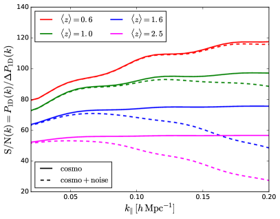
Figure 4: Signal-to-noise ($S/N$) ratio of the radial 21cm power spectrum in our fiducial redshift bins for maps containing only the cosmological signal (solid lines) and the cosmological signal plus system noise (dashed lines) using the cosmological mask. The $S/N$ ratio is defined as the ratio between the amplitude and the error of the radial power spectrum.

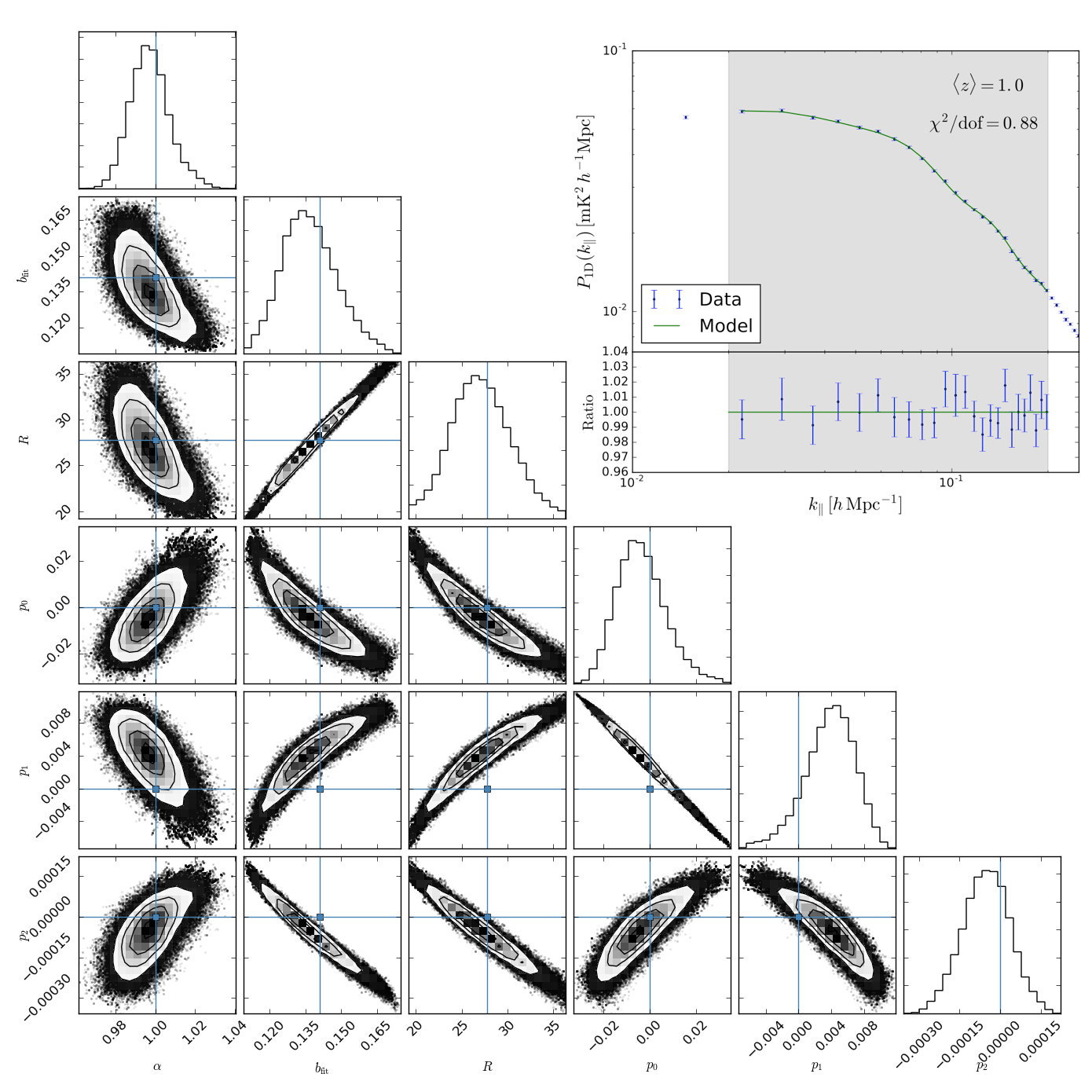
Figure 5: MCMC constraints on the 6 parameters used in the fits to the measured 1D power spectrum for one of the simulations. The results of the simulation (at $\langle z\rangle=1.0$) together with the best fit is shown in the upper-left corner, where the dashed area represents the $k$-range where we perform the fit (residuals shown in the bottom panel). While the BAO parameter $\alpha$ shows no significant correlations with the other parameters, a result of the robustness of the BAO signal, the remaining five parameters show strong degeneracies among themselves. This is due to the fact that all of them affect the amplitude and broadband shape of the power spectrum in a similar way.

z range	$\langle z\rangle$	mask		$\sigma_{\alpha}$
			(C)	(C+N)	(C+N+FG)
[0.36-0.75]	0.6	no	${\color[rgb]{.5,.5,.5}1.008\pm 0.016}$	${\color[rgb]{.5,.5,.5}1.008\pm 0.016}$	${\color[rgb]{.5,.5,.5}1.007\pm 0.016}$
		yes	${\color[rgb]{1,0,0}1.006\pm 0.020}$	${\color[rgb]{1,0,0}1.006\pm 0.021}$	${\color[rgb]{0,0,1}1.006\pm 0.024}$
[0.75-1.26]	1.0	no	${\color[rgb]{.5,.5,.5}0.996\pm 0.010}$	${\color[rgb]{.5,.5,.5}0.997\pm 0.011}$	${\color[rgb]{.5,.5,.5}0.996\pm 0.011}$
		yes	${\color[rgb]{1,0,0}0.997\pm 0.012}$	${\color[rgb]{1,0,0}0.997\pm 0.013}$	${\color[rgb]{0,0,1}0.998\pm 0.015}$
[1.26-1.98]	1.6	no	${\color[rgb]{.5,.5,.5}1.001\pm 0.011}$	${\color[rgb]{.5,.5,.5}1.004\pm 0.014}$	${\color[rgb]{.5,.5,.5}1.003\pm 0.014}$
		yes	${\color[rgb]{1,0,0}1.000\pm 0.013}$	${\color[rgb]{1,0,0}1.003\pm 0.016}$	${\color[rgb]{0,0,1}1.004\pm 0.019}$
[1.98-3.05]	2.5	no	${\color[rgb]{.5,.5,.5}1.004\pm 0.013}$	${\color[rgb]{.5,.5,.5}1.003\pm 0.021}$	${\color[rgb]{.5,.5,.5}1.000\pm 0.021}$
		yes	${\color[rgb]{1,0,0}1.004\pm 0.016}$	${\color[rgb]{1,0,0}1.002\pm 0.026}$	${\color[rgb]{0,0,1}1.002\pm 0.031}$

Table 2: For each simulation we fit the measured radial power spectrum on 4 the redshift bins specified in the first column using the theoretical template of Eq. 22. Columns 4-6 show the mean and standard deviation of the BAO parameter $\alpha$. Constraints are shown for maps containing only the cosmological signal (column 4), the cosmological signal plus instrumental noise (column 5) and the cosmological signal, noise and foreground residuals (column 6). The radial power spectra are measured using all pixels of the maps (gray numbers) or using a mask: the cosmological mask ($f_{\rm sky}=0.72$) and the the foregrounds mask ($f_{\rm sky}=0.58$).

In Fig. 4 we show the signal-to-noise ratio of the radial 21cm power spectrum in the four redshift bins as a function of wavenumber. The curves shown in this figure were computed using the theoretical prediction for the 1D power spectrum and its uncertainty assuming Gaussian statistics, which we have shown to be good approximations to the simulated data (see Appendix C). We considered separately the cases with and without instrumental noise, and in both cases we estimated the errors assuming the volume available for the cosmological mask.

Focusing on the results involving the cosmological signal alone, it can be seen that the $S/N$ decreases towards higher redshifts. This is a-priori surprising, since the volume of the redshift bins increases with its mean redshift. We can understand this by writing the $S/N$ ratio at linear order (see Appendices B and C for the derivation)

$${\rm S/N}(k)=\cfrac{\frac{1}{2\pi}\int_{0}^{\infty}P_{\rm 21cm,3D,obs}(k_{\|},k_{\bot})k_{\bot}dk_{\bot}}{\sqrt{(V\Delta k)^{-1}\int_{0}^{\infty}\left[P_{\rm 21cm,3D,obs}(k_{\|},k_{\bot})+P_{N}\right]^{2}k_{\bot}dk_{\bot}}}$$ (27)

where $V$ is the survey volume and $\Delta k$ is the width of the $k$-bin over which the power spectrum is estimated. $P_{N}$ is the amplitude of the white-noise arising from the instrument temperature and is given in Eq. 35.

Should all 21cm maps have the same angular resolution and no system noise, the $S/N$ ratio would simply scale inversely with the square root of the survey volume. However, the beam size grows at larger wavelenghts, and the corresponding damping exponential factor $\exp(-k_{\bot}^{2}R^{2})$ reduces both the amplitude and the errors of the 1D power spectrum (see Figs. 7 and 11) with increasing $R$ (and therefore redshift). The effect on both quantities is, however, different, and the amplitude of the power spectrum is reduced more efficiently than its errors. That decrease is not compensated by the increase in the survey volume, and the net effect is a reduction in $S/N$ at higher redshifts.

Turning now to maps containing instrumental noise, we can see that, while at low redshift the effects of the noise are almost negligible, in the two highest redshift bins the uncertainties in the power spectrum become dominated by it. This, for instance, produces a dramatic drop in $S/N$ in the $\langle z\rangle=2.5$ redshift bin. This has a direct impact in the final BAO constraints, as we shall see in Section 4.3.

It is worth pointing out that the $S/N$ ratio varies very mildly with wavenumber for the 1D power spectrum in the noiseless case. This is easy to understand: unlike in the case of the isotropic 3D power spectrum, where each $k$-mode is sampled by all ${\bf k}$s inside a spherical shell of radius $k$, in the 1D case only a single mode per pixel contributes to the estimate of the power spectrum at a given $k_{\|}$, and therefore all modes are sampled roughly equally.

4.2 Cosmological signal

For simulations containing only the cosmological signal we fit the measured radial 21cm power spectrum of each redshift bin of each simulation using the template of Eq. 22. An example of the measurements together with the best-fit is shown in the upper-right corner of Fig. 5. From each fit we obtain the value of the BAO parameter $\alpha$ as well as the nuisance parameters together with the corresponding $\chi^{2}$. Fig. 6 shows, with blue lines, the distribution of $\alpha$, $b_{\rm fit}$ and reduced $\chi^{2}$, and the fourth column in Table 2 shows the average value and standard deviation of $\alpha$ obtained from the 100 lognormal realizations. The values obtained for the full sky are displayed in gray, while those corresponding to the cosmological mask are shown in red. We will focus on the latter from now on.

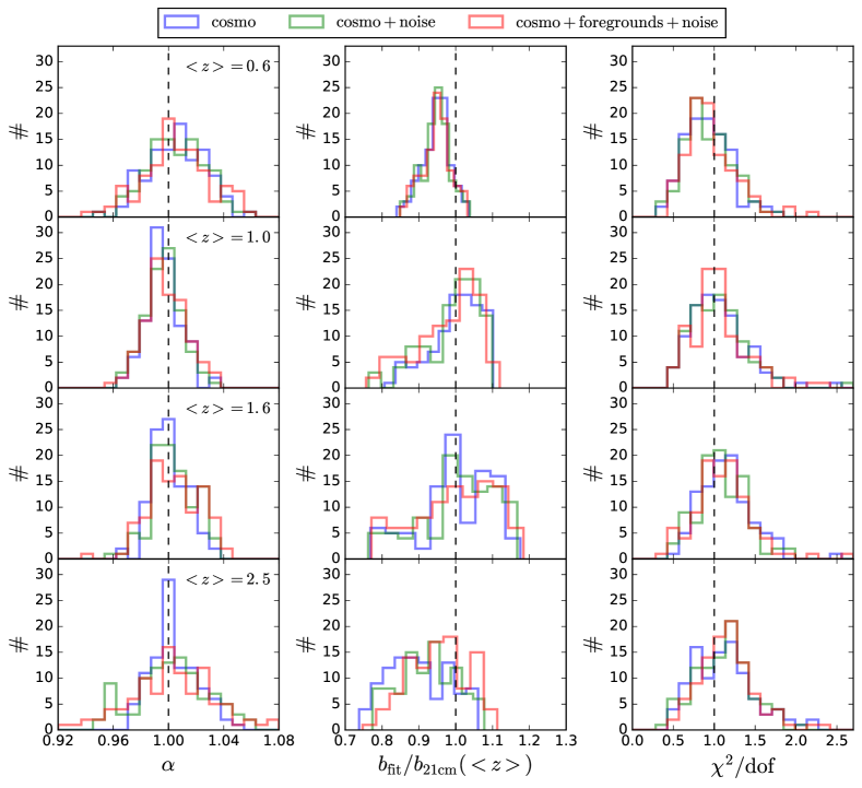
Figure 6: Distribution of the best-fit values of $\alpha$ (left column), $b_{\rm fit}$ (central column) and the corresponding reduced $\chi^{2}$ (right column) for each redshift bin and simulation. Results are shown for the bins with mean redshifts $\langle z\rangle=0.6$ (top), $\langle z\rangle=1.0$ (middle top), $\langle z\rangle=1.6$ (middle bottom) and $\langle z\rangle=2.5$ (bottom). The different line colors correspond to the results for simulations containing only the cosmological signal (blue), cosmological signal plus instrument noise (green) and cosmological signal, instrument noise and foreground residuals (red).

By inspecting the distribution of the best-fit values of $\alpha$ as well as the corresponding reduced $\chi^{2}$ we first verified that our theoretical template is a good model for the data, and that we obtain an unbiased estimate of the true BAO scale. The relative constraints on the Hubble rate are given directly by the error on $\alpha$. In the three high-redshift bins we find $\sigma_{\alpha}=1.2\%-1.6\%$, while the lowest redshift bin shows a significantly larger error ($\sigma_{\alpha}=2.0\%$). The constraints on $\alpha$ improve by $\sim 20\%$ when using the full sky, in agreement with the corresponding increase in sky area and therefore survey volume.

The magnitude of the errors on $\alpha$ and its redshift dependence can be understood taking the two effects discussed in Sections 2.2 and 4.5: the $S/N$ ratio of the signal and the significance of the BAO wiggles. While the $S/N$ decreases with redshift (see Fig. 4), the significance of the BAO increases with it (see Fig. 2). The BAO wiggles are less significant on the radial power spectrum at low redshift, which increases the uncertainties on $\alpha$, and therefore we expect these uncertainties to increase towards lower redshifts. On the other hand, the significance of the BAO signal saturates at high redshift, while the $S/N$ ratio continues to decrease with redshift, and thus we would expect the error on $\alpha$ to grow at higher redshifts as well. This agrees with the trend observed in the data. The most precise determination of $\alpha$ is obtained in the two intermediate redshift bins.

Before moving on to more realistic simulations, it is worth noting that, while the parameter $b_{\rm fit}$ can in principle be interpreted as the bias of the 21cm signal ($b_{\rm fit}\propto b_{\rm HI}\Omega_{\rm HI}$), it is not clear that the method used in this paper would yield an unbiased estimate of this quantity. The main reason for this is the strong degeneracies existing between this parameter and the nuisance parameters $R$ and $p_{i}$ (see Fig. 5), all of which affect the overall normalization and broad-band shape of the power spectrum. Furthermore, unlike the case of the BAO signature, nothing would prevent us from using the full three-dimensional clustering information to constrain this parameter, and therefore using the 1D power spectrum to measure $b_{\rm HI}$ would be, in any case, sub-optimal. Nevertheless, the histograms shown in the central panels of Figure 6 show that the recovered values of $b_{\rm 21cm}$ are, on average, in good agreement with the input model.

4.3 System noise

We now study the impact of the instrument temperature on our results. As shown in Appendix B, the noise contribution to the total power spectrum increases with redshift, and in fact, eventually dominates the cosmological signal at low frequencies. We can therefore expect a non-negligible effect on the detectability and uncertainties of the BAO signal.

In order to avoid a noise bias in the computation of the 1D power spectrum, for each sky simulation we generate two realizations of the instrumental noise, add them to the simulation and compute the 1D power spectrum as the cross-correlation of the two resulting sets of maps. This simulates the way in which power spectra would be estimated in a realistic setting, by taking cross-correlations of different data splits. Fig. 7 shows the 1D power spectra computed in the four redshift bins of one of our simulations. The solid lines show the power spectrum computed for a simulation containing only the cosmological signal, while the dashed lines include the effects of instrumental noise, which can be observed as a random scatter around the noiseless lines with a relative variance that grows towards smaller scales. The dotted lines in Figure 7 illustrate the noise bias induced when auto-correlating maps with the same noise realization, and explicitly shows the growing contribution of the instrumental noise towards higher redshifts. This was also illustrated in Figure 4.

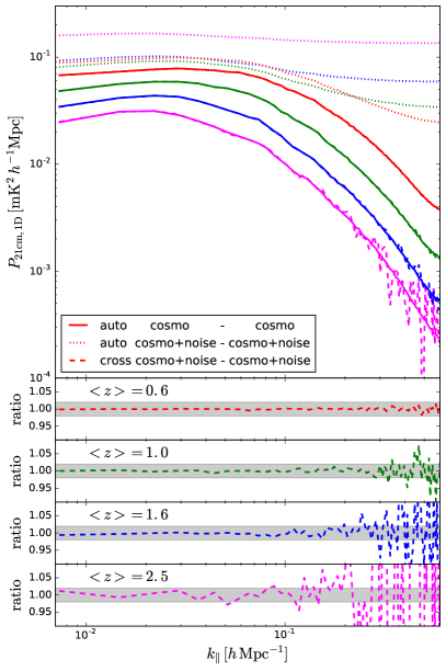
Figure 7: Impact of system noise on the measured radial 21cm power spectrum. The solid lines show the power spectrum measured in one simulation containing only the cosmological signal. The dotted lines display the results obtained by measuring the power spectrum in maps that contain both the cosmological signal and the system noise. The dashed lines present the results obtained by computing the cross-power spectrum from two different noise realizations with the same cosmological signal. The power spectra are measured in four different redshift bins: $\langle z\rangle=0.6$ (purple), $\langle z\rangle=1.0$ (blue), $\langle z\rangle=1.6$ (green), $\langle z\rangle=2.5$ (red). The bottom panels show the ratio between dashed and solid lines and shaded regions represent a $2\%$ difference.

For each simulation and redshift bin we have fit the radial 21cm power spectrum measured employing the above procedure to the theoretical template of Eq. 22. From each fit we measure the value of $\alpha$ and $\chi^{2}$ and in Fig. 6 we show their distribution in green lines from the 100 realizations for the four different redshift bins. Table 2 summarizes, in the fifth column, the mean and standard deviation of the distribution. We find that the instrumental noise increases the uncertainty on the BAO parameter by $5\%,8\%,23\%\,\text{and}\,64\%$ in the bins with mean redshift $0.6,1.0,1.6\,\text{and}\,2.5$ respectively. The large degradation in the BAO signal in the higher redshift bin is, as explained above, a consequence of the larger instrumental noise present in that bin. It is worth noting that the uncertainties on the overall scaling of the power spectrum, given by the effective bias $b_{\rm fit}$ experience a much milder variation after introducing instrumental noise. This is due to the fact that most of the constraining power for this parameter comes from the largest scales, where cosmic variance dominates in all bins.

Table 2 also shows, in gray, the mean values and standard deviations for full-sky observations. We should clarify that, in this case, we fixed the observing time per pixel, thus assuming that the total allocated observation time would scale with $f_{\rm sky}$. The improvement in the constraints is thus solely due to the increase in surveyed volume.

4.4 Foregrounds

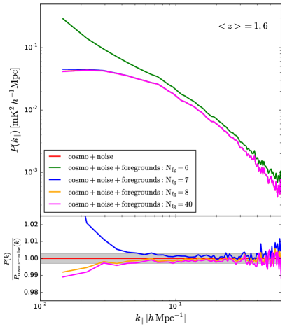
Figure 8: Radial 21cm power spectrum after foreground cleaning for one particular simulation in the third redshift bin $\langle z\rangle=1.6$. The green, blue, orange and magenta lines correspond to the result of applying a PCA algorithm removing $N_{\rm fg}=6$, 7, 8 and 40 principal components. The red solid line shows the result for simulations containing only cosmological signal and instrumental noise. The bottom panel shows the ratio of the foreground-cleaned power spectra to the result of the foreground-free simulation.

We now study the impact of the presence of Galactic and extra-Galactic foregrounds on our results. We added simulations of the most relevant radio foreground sources to each sky realization as described in Section 3.1 before applying the instrumental beam and noise. As can be seen in Fig. 3 the amplitude of the foregrounds is several orders of magnitude higher than the one from the cosmological signal. We then applied a PCA blind cleaning algorithm to each simulation as described in Section 3.2 (this was done independently for the two noise realizations per simulation described in the previous section).

Figure 8 shows the performance of the foreground cleaning method. The method is based on subtracting a number $N_{\rm fg}$ of principal components from the maps, with the hope that the remaining intensity is dominated by the cosmological signal. The figure shows the radial power spectrum in the third redshift bin ($\langle z\rangle=1.6$) for one particular sky simulation after having applied a PCA algorithm with different values of $N_{\rm fg}$ ($N_{\rm fg}=6$ in green, 7 in blue, 8 in orange and 40 in magenta). For comparison the figure also contains, in red, the power spectrum of the foregrounds-free simulation. It is worth noting that, as described in Bigot-Sazy et al. (2015), the effects of correlated instrumental noise, of particular relevance for single-dish experiments such as SKA1-MID (Harper et al., 2016), would also be partially removed by the foreground-cleaning algorithm. As the figure shows, the procedure works remarkably well due to the very different spectral characteristics of signal and foregrounds. We find that the presence of foreground residuals can be minimized after subtracting $N_{\rm fg}=8$ principal components. Note that, inevitably, this method removes part of the cosmological signal, particularly on the largest radial scales dominated by foregrounds. This causes a bias in the radial power spectrum that, however small, could potentially affect the recovery of the BAO scale. This scale-dependent bias is evident in the lower panel of Figure 8, which shows the ratio of the recovered power spectra with respect to the foreground-less case.

Using the above procedure we calculated the radial 21cm power spectrum in each redshift and simulation and we fit the results using the template of Eq. 22. We note that in this case we applied the optimal Galactic mask described in Section 3.1, corresponding to sky fraction $f_{\rm sky}=0.58$. Fig. 6 shows, in red, the distribution of the fit parameters $\alpha$ and $b_{\rm fit}$, as well as the values of the reduced $\chi^{2}$ for our 100 simulations. The corresponding mean value and standard deviation of $\alpha$ for simulations containing foregrounds are reported in the sixth column of Table 2. As expected, we find that the errors on $\alpha$ increase with respect to the results found in the foreground-free simulations. The error enhancement is roughly $\sim 20\%$, and is mainly caused by the smaller sky area allowed by the Galactic mask. More importantly, we find that as expected, the small foreground bias on large scales mentioned above does not bias the recovered values of the BAO scaling parameter. Note that, as pointed out in Alonso et al. (2015), the power spectrum uncertainties are also expected to receive a contribution from foreground residuals, however, this effect is subdominant. We thus conclude that, for well-behaved foregrounds, SKA1-MID should be able to measure the radial BAO scale with good accuracy up to redshifts $z\sim 3$.

4.5 BAO significance

Besides placing constraints on the scale of the BAO, it is also important to determine the significance with which the signature has been detected in the power spectrum.

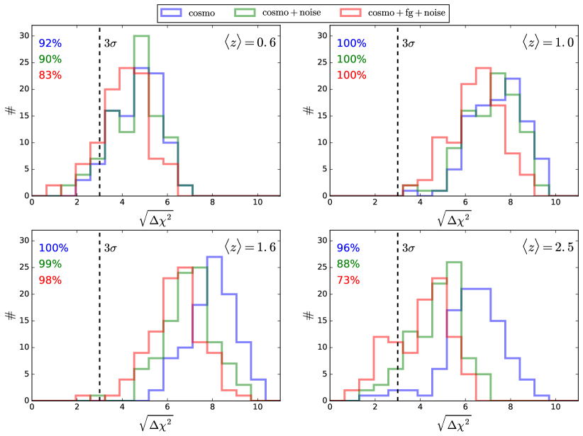
Figure 9: Significance of the BAO wiggles in each redshift bin for maps containing only the cosmological signal (blue), the cosmological signal plus system noise (green) and the cosmological signal, noise and foregrounds (red). The histograms show the distribution of the square root of the increment in $\chi^{2}$ between our fiducial model for the radial power spectrum (Eq. 22) and a no-BAO template. Thus the $x$-axis can be read as the “number of sigmas” with which the BAO have been detected. The vertical dashed lines show the $3\sigma$ threshold, and we provide, in each case, the number of simulations with a significance above this threshold.

We have done so through the following procedure. For each simulation and redshift bin we measure the radial 21cm power spectrum and then fit the results using a no-BAO template for the power spectrum:

$$P_{\rm model}(k_{\|},z|\mn@boldsymbol{\Theta})=P_{\rm nw,1D}(k_{\|},z)+p_{0}k_{\|}+p_{1}+p_{2}/k_{\|}~{}.$$ (28)

We then compared the $\chi^{2}$ value of the fits with and without the BAO contribution, and quantified the significance of the BAO detection in terms of the increment between both cases, $\Delta\chi^{2}$. Fig. 9 shows the histograms for the values of $\sqrt{\Delta\chi^{2}}$ from each redshift bin and simulation, for maps containing just the cosmological signal (blue lines), the cosmological signal plus system noise (green lines) and the cosmological signal, noise and foreground residuals (red lines).

We find that, although in the higher-redshift bin a relatively large fraction ($\sim 27\%$) of the simulations yield BAO detections below the $3\sigma$ threshold, it is generally likely, in all cases, to make a reliable measurement ($>3\sigma$) of the radial BAO signature. As explained above, the main reason for the lower significance of the BAO measurements in the highest redshift bin is the larger system noise at low frequencies. It is also worth noting that the first redshift bin generally yields lower-significance detections than the next two. As discussed in Section 2.2, this is caused by the larger contribution from small angular scales in the lower redshift bin, which reduce the relative contribution from the BAO wiggles to the radial power spectrum. This can be visualized explicitly in Fig. 10, which shows the best-fit power spectra with and without BAO in the 4 different redshift bins for one particular simulation in the absence of noise or foreground contamination.

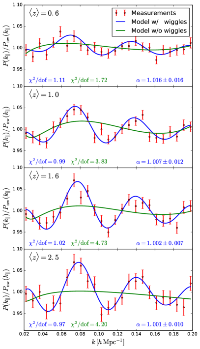
Figure 10: The red points represent measurements of the radial power spectrum in different redshift bins from one particular simulation. The error bars of the red points represent the error on the measurements. The blue/green lines display the best-fit model from a theoretical template with/without BAO wiggles. Both the measurements and the best-fit models are normalized by a model without BAO wiggles with fixed parameters.

5 Conclusions

The BAO scale is one of the most robust cosmological observables, due to the distinctive nature of their signature, a single peak on the 2pt correlation function or a set of wiggles on the power spectrum. This observable can be used to measure the Hubble function and the angular diameter distance as a function of redshift, and therefore represents a unique and robust probe to study the nature of dark energy.

The purpose of this paper has been to investigate the accuracy with which the BAO scale can be determined through single-dish 21cm intensity mapping observations in the post-reionization epoch. We quote results for a possible intensity mapping experiment carried out with the SKA1-MID array covering more than half of the sky in the redshift range $z\sim[0.3-3]$. We however emphasize that our methodology is fully general and can be easily applied to other instruments.

We have shown that the smearing caused by the beam size of the radio-telescopes will prevent a competitive measurement of the isotropic BAO scale in both the 21cm correlation function or power spectrum (see Fig. 1). However, we have shown that, given the good frequency resolution of radio telescopes, it should still be possible to measure the radial BAO signal down to high redshifts, thus placing competitive constraints on the expansion rate $H(z)$.

In this paper we have proposed a method to recover the radial BAO scale in intensity mapping observations and implemented it in practice making use of a suite of 100 full-sky lightcone simulations in order to systematically study the effects of the instrumental noise and the robustness of the signal to foreground-related systematic effects. Our procedure follows three steps:

• A simulated sky is generated containing a realization of the full-sky HI cosmological signal as well as the most relevant Galactic and extra-Galactic foregrounds in the frequency range $\nu\in[350,1050]\,{\rm MHz}$. The simulated maps are smoothed to the angular resolution corresponding to the specifications of SKA1-MID, and white instrumental noise is added accordingly.

• We remove the foregrounds using a PCA algorithm, subtracting the first 8 principal components, which we have shown are dominated by foregrounds.

• We compute the radial power spectrum of the resulting maps by stacking the 1-dimensional Fourier transform of every pixel in the field of view along the frequency direction (further details about the method are given in Section 3.3).

• For each estimated power spectrum, we determine the radial BAO scaling parameter $\alpha$ by fitting the template given in Eq. 22 to the data. The mean value and uncertainty on $\alpha$ is then estimated by averaging over 100 simulations.

All our simulations take into account the sky area limitations of the SKA both in terms of accessible sky and Galactic foregrounds.

Our results concerning the measurement of the BAO scale are summarized in Table 2. We find that the BAO uncertainties become larger at both high and low redshifts, even in the absence of instrumental noise. We have shown that this is due to the low relative amplitude of the BAO signature in the radial power spectrum at low redshifts and to the lower signal-to-noise ratio of the total HI power spectrum at high redshifts caused by the larger size of the telescope beam, which overcomes the $\propto 1/\sqrt{V}$ improvement factor due to the larger volume coverage. More importantly, we find that, while the effects of instrumental noise are irrelevant at low redshift, they come to dominate the error budget at redshifts $z\gtrsim 2$, increasing the final BAO uncertainties by a factor of $\sim 2$ with respect to the sample-variance limited result.

Concerning the effect of radio foregrounds, we have shown that the large-scale bias induced by foreground removal on the radial power spectrum (as reported by e.g. Alonso et al. (2015)) does not cause a bias in the recovered BAO scale. This is thanks to the robustness of the BAO signal against broad-band variations in the shape of the power spectrum, as well as to the spectral separation between foregrounds and cosmological signal in the frequency direction. We have also shown that the contribution of foreground residuals to the final uncertainties is negligible, and that, therefore, the main effect of foregrounds is a reduction in the available sky area needed in order to avoid the regions of higher Galactic emission. Although we have not explicitly introduced this effect, it should be possible to mitigate the impact of correlated instrumental noise, of particular relevance to single-dish observations, using similar methods (Bigot-Sazy et al., 2015).

Finally, we have studied the significance of the BAO signal. We have shown that, although the large variance of the instrumental noise at low frequencies reduces the signal-to-noise ratio of the BAO signature at high redshifts, we obtain significant detections ($>3\sigma$) of it in a large majority of our simulations in all redshift bins.

Overall, we conclude that by a single-dish 21cm intensity mapping experiment carried out by SKA1-MID over $\sim 50\%$ of the sky with an allocated observing time of 10000 hours should be able to place direct constrains the value of the Hubble function $H(z)$ with a relative uncertainty of $(2.4\%,1.5\%,1.9\%,3.1\%)$ at redshifts $\langle z\rangle=(0.6,1.0,1.6,2.5)$ by measuring the BAO scale in the radial 21cm power spectrum. This would correspond to a precision comparable with next-generation spectroscopic surveys (e.g. Font-Ribera et al. (2014)).

Appendix A HI model

It has been shown in Villaescusa-Navarro et al. (2014) that the abundance of HI outside dark matter halos is negligible and that its contribution to the amplitude of the 21cm power spectrum can be safely neglected. Under those conditions, it is possible to model the clustering properties of HI using the halo model framework. A key element in that formalism is the function $M_{\rm HI}(M,z)$, that outputs the average HI mass that a dark matter halo of mass $M$ has at redshift $z$. If this function is known, it is possible to compute the two basic elements needed to estimate the shape and amplitude of the 21cm power spectrum at linear order, $\Omega_{\rm HI}(z)$ and $b_{\rm HI}$:

$$\Omega_{\rm HI}(z) = \frac{1}{\rho_{c}^{0}}\int_{0}^{\infty}n(M,z)M_{\rm HI}(M,z)dM$$ (29)

$$b_{\rm HI}(z) = \frac{1}{\rho_{c}^{0}\Omega_{\rm HI}(z)}\int_{0}^{\infty}b(M,z)n(M,z)M_{\rm HI}(M,z)dM$$

where $\rho_{c}^{0}$ is the critical density of the Universe today and $n(M,z)$ and $b(M,z)$ are the halo mass function and halo bias at redshift $z$.

Villaescusa-Navarro et al. (2016) used zoom-in hydrodynamical simulations to show that the high mass end of the $M_{\rm HI}(M,z)$ can be modeled by a simple power law: $M_{\rm HI}(M,z)\propto M^{3/4}$. In the low-mass end Villaescusa-Navarro et al. (2015) found a similar behavior for many different cosmological models. We therefore model the $M_{\rm HI}(M,z)$ function as

$$M_{\rm HI}(M,z)=e^{\gamma(z)}M^{3/4}\exp\left(-(M_{\rm min}(z)/M)^{2}\right)$$ (30)

where $e^{\gamma(z)}$ represents an overall normalization and the exponential cut-off at the characteristic halo mass $M_{\rm min}(z)$ is introduced to model the fact that it is expected that low-mass halos should not host a significant amount of HI (Pontzen et al., 2008; Marín et al., 2010; Bagla et al., 2010; Villaescusa-Navarro et al., 2014; Padmanabhan et al., 2016). For simplicity we consider that the characteristic cut-off scale $M_{\rm min}(z)$ does not depend on redshift.

Our model has two free parameters: $M_{\rm min}$ and $\gamma(z)$. The value value of $\gamma(z)$ is fixed by requiring that our model reproduce the relation $\Omega_{\rm HI}(z)=4\times 10^{-4}(1+z)^{0.6}$ inferred from observations in Crighton et al. (2015). The value of $M_{\rm min}=1.7\times 10^{10}~{}h^{-1}M_{\odot}$ is chosen such as our model reproduces the value of $\Omega_{\rm HI}b_{\rm HI}=(0.62^{+0.23}_{-0.15})\times 10^{-3}$ at $z\simeq 0.8$ derived from 21cm intensity mapping observations in Switzer et al. (2013).

The HI bias that we obtain with the above model can be well described in the redshift range $z\in[0,3]$ by the following relation

$$b_{\rm HI}(z)=0.904+0.135(1+z)^{1.696}~{}.$$ (31)

We notice that our model reproduces, by construction, the $\Omega_{\rm HI}(z)$ relation, while at $z=0.8$ it predicts a value of $\Omega_{\rm HI}b_{\rm HI}=7.2\times 10^{-4}$, in perfect agreement with the constraints from Switzer et al. (2013). Besides, at $z=2.3$ it predicts a HI bias equal to $b_{\rm HI}=1.93$, compatible with the measured DLAs bias by Font-Ribera et al. (2012), $b_{\rm DLAs}(z=2.3)=2.17\pm 0.2$, assuming that bias of the DLAs is a good proxy for the HI bias.

Appendix B Noise power spectrum

The aim of this appendix is to compute the theoretical noise contribution to the total power spectrum. We start by noting that an uncorrelated Gaussian random field $n$ has a white power spectrum given by

$$\langle\delta_{\bf k}\delta^{*}_{\bf q}\rangle=\delta^{\cal D}({\bf k}-{\bf q})\,v_{\rm cell}\sigma_{\rm cell}^{2},$$ (32)

where $\sigma_{\rm cell}^{2}$ is the variance of the field in cells of volume $v_{\rm cell}$.

On the other hand, the instrumental noise variance per pixel is given by

$$\sigma^{2}_{\rm pix}=\frac{T_{\rm sys}^{2}}{2\Delta\nu\,t_{\rm pix}\,N_{\rm dish}},$$ (33)

where $T_{\rm sys}$ is the system temperature, $\Delta\nu$ is the frequency interval, $t_{\rm pix}$ is the observation time per pixel and $N_{\rm dish}$ is the number of antennas. $t_{\rm pix}$ can be related to the pixel solid angle as $t_{\rm pix}=\Omega_{\rm pix}\,t_{\rm tot}/(4\pi\,f_{\rm sky})$, where $t_{\rm tot}$ is the total observation time. Moreover, the frequency interval $\Delta\nu$ and the pixel solid angle $\Omega_{\rm pix}$ can be related to the comoving volume covered by each pixel as

$$\Delta\nu\,\Omega_{\rm pix}=\frac{H\,\nu_{\rm 21}}{r^{2}\,(1+z)^{2}}\,v_{\rm pix},$$ (34)

where $r$ and $H$ are the comoving distance and the expansion rate.

Thus, combining Equations 33 and 34 we obtain the noise power spectrum

$$P_{N}=T_{\rm sys}^{2}\frac{4\pi\,f_{\rm sky}[(1+z)\,r]^{2}}{2\,t_{\rm tot}\nu_{21}N_{\rm dish}H}.$$ (35)

Appendix C Covariance matrix

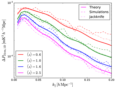
Figure 11: 1$\sigma$ uncertainties on the radial 21cm power spectrum estimated from the theoretical Gaussian prediction (solid lines), as the standard deviation of the 100 lognormal realizations (dashed lines) and using the Jackknife technique over one single realization (dot-dashed lines). Results are shown for the four fiducial redshift bins we use in our analysis.

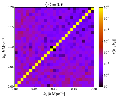
Figure 12: Absolute value of the correlation coefficient matrix of the radial power spectrum in the $\langle z\rangle=0.6$ redshift bin estimated from 100 lognormal realizations.

In order to validate the uncertainties on the radial power spectrum used in the analysis of this work we have compared the results from three different methods: 1) the expected Gaussian errors, 2) the r.m.s. from our 100 simulations and 3) the errors estimated using the Jackknife method.

We begin by describing the computation of the expected Gaussian errors. Throughout this Section we will make use of the flat-sky approximation. The basic observable in our analysis is the HI overdensity field Fourier-transformed along the line of sight (labelled by $\parallel$ here):

$$\delta(k_{\parallel},{\bf r}_{\perp})\equiv\int\frac{dr_{\parallel}}{\sqrt{2\pi}}\,\delta(r_{\parallel},{\bf r}_{\perp})\,e^{ik_{\parallel}r_{\parallel}}.$$ (36)

As we described above, the 1D power spectrum is estimated by averaging the radial power spectrum across all lines of sight independently. Thus, our estimator is:

$$\hat{P}_{\rm 1D}(k_{\parallel})=\frac{2\pi}{L}\int\frac{d^{2}r_{\perp}}{A}\left|\delta(k_{\parallel},{\bf r}_{\perp})\right|^{2},$$ (37)

where $L$ and $A$ are the comoving depth and area of the region covered by the intensity mapping experiment, and the factor $2\pi/L$ accounts for the Dirac’s delta normalization of the power spectrum in a region of finite size.

Now, assuming that the HI overdensity is Gaussianly distributed, we can use Wick’s theorem to show that the covariance of this estimator is given by

$$C(k_{\parallel},k_{\parallel}^{\prime}) \equiv\left\langle\left(\hat{P}_{\rm 1D}(k_{\parallel})-P_{\rm 1D}(k_{\parallel})\right)\left(\hat{P}_{\rm 1D}(k_{\parallel}^{\prime})-P_{\rm 1D}(k_{\parallel}^{\prime})\right)\right\rangle$$

$$=\frac{\delta^{\cal D}(k_{\parallel}-k_{\parallel}^{\prime})}{V}\int_{0}^{\infty}dk_{\perp}\,k_{\perp}\,P_{\rm 3D}^{2}(k_{\parallel},k_{\perp}),$$ (38)

where $V\equiv L\,A$, and $\delta^{\cal D}$ is the Dirac delta function. Since we measure the 1D power spectrum in finite intervals of $k_{\parallel}$ of width $\Delta k_{\parallel}$, we can substitute $\delta^{\cal D}(k_{\parallel}-k_{\parallel}^{\prime})\rightarrow\delta^{\cal K}(k_{\parallel},k_{\parallel}^{\prime})/\Delta k_{\parallel}$, where $\delta^{\cal K}$ is the Kronecker delta. Thus we find that, in the Gaussian approximation, the uncertainties on the 1D power spectrum are purely diagonal and given by

$${\rm Var}\left[P_{\rm 1D}(k_{\parallel})\right]=\frac{1}{V\Delta k_{\parallel}}\int_{0}^{\infty}dk_{\perp}\,k_{\perp}\,P_{\rm 3D}^{2}(k_{\parallel},k_{\perp})~{}.$$ (39)

We conclude by noting that, in the presence of noise, $P_{\rm 3D}$ above must be understood to contain contributions from both the cosmological signal and the instrumental noise. Taking into account the pixel window function this then reads:

$$P_{\rm 3D}^{2}(k_{\parallel},k_{\perp})=W^{2}_{p}(k_{\perp})\left[P_{\rm 21cm}(k_{\parallel},k_{\perp})+P_{N}\right],$$ (40)

where the noise power spectrum $P_{N}$ is given in Eq. 35.

Figure 11 shows this theoretical prediction compared with the standard deviation of the 100 lognormal realizations and the error estimation from one single realization using the Jackknife method. We show the results for the 4 fiducial frequency bins used in the BAO analysis. We conclude that the error estimations from the three different methods are in very good agreement among themselves. We notice however that there are non-negligible deviations in the highest frequency bin (lowest redshifts) on small scales (large $k_{\parallel}$), which can be ascribed to the effect of the non-linearities induced by the lognormal transformation. We also find that errors computed using the Jackknife method tend to be systematically lower than those obtained from the other two methods. Figure 12 shows the absolute value of the correlation matrix,

$$r(k_{1},k_{2})=\frac{C(k_{1},k_{2})}{\sqrt{C(k_{1},k_{1})C(k_{2},k_{2})}}~{},$$ (41)

measured on the most non-linear redshift bin: $z\in[0.36-0.75]$ from the 100 lognormal realizations. As can be seen, the non-diagonal elements of the covariance matrix are negligible, which justifies our use of purely diagonal errors.

We therefore conclude that the covariance matrix of the radial 21cm power spectrum, in the redshifts and $k-$range relevant for this paper, can be accurately approximated by a diagonal matrix, whose elements can be found by employing the theoretical Gaussian prediction, the standard deviation of different realizations or internal methods such as Jackknife. The results presented in this papers were obtained using errors computed from the 100 lognormal realizations.

References

- Alam et al. (2016) Alam S. et al., 2016, ArXiv e-prints, arXiv:1607.03155
- Alonso et al. (2015) Alonso D., Bull P., Ferreira P. G., Santos M. G., 2015, MNRAS, 447, 400, arXiv:1409.8667
- Alonso et al. (2014) Alonso D., Ferreira P. G., Santos M. G., 2014, MNRAS, 444, 3183, arXiv:1405.1751
- Anderson et al. (2014) Anderson L. et al., 2014, MNRAS, 439, 83, arXiv:1303.4666
- Bagla et al. (2010) Bagla J. S., Khandai N., Datta K. K., 2010, MNRAS, 407, 567, arXiv:0908.3796
- Baldauf et al. (2015) Baldauf T., Mirbabayi M., Simonović M., Zaldarriaga M., 2015, PRD, 92, 043514, arXiv:1504.04366
- Battye et al. (2012) Battye R. A. et al., 2012, ArXiv e-prints, arXiv:1209.1041
- Battye et al. (2004) Battye R. A., Davies R. D., Weller J., 2004, Mon.Not.Roy.Astron.Soc., 355, 1339, arXiv:astro-ph/0401340
- Beutler et al. (2016) Beutler F. et al., 2016, ArXiv e-prints, arXiv:1607.03149
- Bharadwaj et al. (2001) Bharadwaj S., Nath B. B., Sethi S. K., 2001, Journal of Astrophysics and Astronomy, 22, 21, arXiv:astro-ph/0003200
- Bharadwaj & Sethi (2001) Bharadwaj S., Sethi S. K., 2001, Journal of Astrophysics and Astronomy, 22, 293, arXiv:astro-ph/0203269
- Bigot-Sazy et al. (2015) Bigot-Sazy M.-A. et al., 2015, MNRAS, 454, 3240, arXiv:1507.04561
- Braun et al. (2015) Braun R., Bourke T. L., Green J. G., Keane E. F., Wagg J., 2015, in PoS ed., Advancing Astrophysics with the Square Kilometre Array. PoS(AASKA14)174
- Bull et al. (2015a) Bull P., Ferreira P. G., Patel P., Santos M. G., 2015a, ApJ, 803, 21, arXiv:1405.1452
- Bull et al. (2015b) Bull P., Ferreira P. G., Patel P., Santos M. G., 2015b, ApJ, 803, 21, arXiv:1405.1452
- Carucci et al. (2015) Carucci I. P., Villaescusa-Navarro F., Viel M., Lapi A., 2015, Journal of Cosmology and Astroparticle Physics, 7, 047, arXiv:1502.06961
- Chang et al. (2008) Chang T.-C., Pen U.-L., Peterson J. B., McDonald P., 2008, Physical Review Letters, 100, 091303, arXiv:0709.3672
- Cole et al. (2005) Cole S. et al., 2005, MNRAS, 362, 505, arXiv:astro-ph/0501174
- Crighton et al. (2015) Crighton N. H. M. et al., 2015, MNRAS, 452, 217, arXiv:1506.02037
- Crocce & Scoccimarro (2008) Crocce M., Scoccimarro R., 2008, PRD, 77, 023533, arXiv:0704.2783
- Delubac et al. (2015) Delubac T. et al., 2015, A&A, 574, A59, arXiv:1404.1801
- Eisenstein & Hu (1998) Eisenstein D. J., Hu W., 1998, ApJ, 496, 605, arXiv:astro-ph/9709112
- Eisenstein et al. (2005) Eisenstein D. J. et al., 2005, ApJ, 633, 560, arXiv:astro-ph/0501171
- Font-Ribera et al. (2014) Font-Ribera A., McDonald P., Mostek N., Reid B. A., Seo H.-J., Slosar A., 2014, Journal of Cosmology and Astroparticle Physics, 5, 023, arXiv:1308.4164
- Font-Ribera et al. (2012) Font-Ribera A. et al., 2012, Journal of Cosmology and Astroparticle Physics, 11, 59, arXiv:1209.4596
- Foreman-Mackey et al. (2013) Foreman-Mackey D., Hogg D. W., Lang D., Goodman J., 2013, PASP, 125, 306, arXiv:1202.3665
- Gil-Marín et al. (2016) Gil-Marín H. et al., 2016, MNRAS, 460, 4210, arXiv:1509.06373
- Górski et al. (2005) Górski K. M., Hivon E., Banday A. J., Wandelt B. D., Hansen F. K., Reinecke M., Bartelmann M., 2005, ApJ, 622, 759, arXiv:astro-ph/0409513
- Harper et al. (2016) Harper S. E., Dickinson C., Battye R., Olivari L., 2016, ArXiv e-prints, arXiv:1606.09584
- Haslam et al. (1982) Haslam C. G. T., Salter C. J., Stoffel H., Wilson W. E., 1982, Astronomy and Astrophysics, Supplement, 47, 1
- Kaiser (1987) Kaiser N., 1987, MNRAS, 227, 1
- Kitaura et al. (2016) Kitaura F.-S. et al., 2016, Physical Review Letters, 116, 171301, arXiv:1511.04405
- Loeb & Wyithe (2008) Loeb A., Wyithe J. S. B., 2008, Physical Review Letters, 100, 161301, arXiv:0801.1677
- Marín et al. (2010) Marín F. A., Gnedin N. Y., Seo H.-J., Vallinotto A., 2010, ApJ, 718, 972, arXiv:0911.0041
- McQuinn et al. (2006) McQuinn M., Zahn O., Zaldarriaga M., Hernquist L., Furlanetto S. R., 2006, ApJ, 653, 815, arXiv:astro-ph/0512263
- Padmanabhan et al. (2016) Padmanabhan H., Choudhury T. R., Refregier A., 2016, MNRAS, 458, 781, arXiv:1505.00008
- Padmanabhan & White (2009) Padmanabhan N., White M., 2009, PRD, 80, 063508, arXiv:0906.1198
- Peloso et al. (2015) Peloso M., Pietroni M., Viel M., Villaescusa-Navarro F., 2015, Journal of Cosmology and Astroparticle Physics, 7, 001, arXiv:1505.07477
- Planck Collaboration et al. (2014) Planck Collaboration et al., 2014, A&A, 571, A16, arXiv:1303.5076
- Pontzen et al. (2008) Pontzen A. et al., 2008, MNRAS, 390, 1349, arXiv:0804.4474
- Santos et al. (2015) Santos M. et al., 2015, Advancing Astrophysics with the Square Kilometre Array (AASKA14), p. 19, arXiv:1501.03989
- Santos et al. (2005) Santos M. G., Cooray A., Knox L., 2005, ApJ, 625, 575, arXiv:astro-ph/0408515
- Slepian et al. (2016) Slepian Z. et al., 2016, ArXiv e-prints, arXiv:1607.06097
- Switzer et al. (2013) Switzer E. R. et al., 2013, MNRAS, 434, L46, arXiv:1304.3712
- Veropalumbo et al. (2016) Veropalumbo A., Marulli F., Moscardini L., Moresco M., Cimatti A., 2016, MNRAS, 458, 1909, arXiv:1510.08852