The NuSTAR X-ray Spectrum of Hercules X-1: A Radiation-Dominated Radiative Shock

Abstract

We report new spectral modeling of the accreting X-ray pulsar Hercules X-1. Our radiation-dominated radiative shock model is an implementation of the analytic work of Becker & Wolff on Comptonized accretion flows onto magnetic neutron stars. We obtain a good fit to the spin-phase averaged 4 to 78 keV X-ray spectrum observed by the Nuclear Spectroscopic Telescope Array during a main-on phase of the Her X-1 35-day accretion disk precession period. This model allows us to estimate the accretion rate, the Comptonizing temperature of the radiating plasma, the radius of the magnetic polar cap, and the average scattering opacity parameters in the accretion column. This is in contrast to previous phenomenological models that characterized the shape of the X-ray spectrum but could not determine the physical parameters of the accretion flow. We describe the spectral fitting details and discuss the interpretation of the accretion flow physical parameters.

1 Introduction

In the standard model for accreting X-ray pulsars, the matter flows from a companion star either via a stellar wind or Roche lobe overflow into an accretion disk around a spinning highly magnetic neutron star (NS). As the orbiting matter approaches the NS, the increased magnetic field strength constrains the material to flow along the magnetic field lines of the assumed NS dipolar field toward one or both of the NS magnetic poles ($B\geq 10^{12}$ Gauss). This plasma falls onto the NS surface at a considerable fraction (up to $\sim$0.5) of the speed of light, giving up its kinetic energy before it merges with the NS surface. Observed X-ray luminosities for these pulsars range from $10^{34-35}$ ergs s^-1 for X  Per (di Salvo et al., 1998), to near the Eddington limit ($\geq 10^{38}$ergs s^-1) for LMC X-4 (Levine et al., 1991), to possibly super-Eddington ($\geq 5\times 10^{39}$ergs s^-1) for ULX M82 X$-$2 (Bachetti et al., 2014).

The physical processes involved in stopping the accreting plasma flow as it merges onto the NS are varied. In the case of low-luminosity accretion, Langer & Rappaport (1982) invoked a collisionless shock above the NS surface to slow the flow to subsonic velocities. Gas pressure then causes the flow to settle sub-sonically onto the NS surface. However, there has always been doubt about the ability of a shock to form in the presence of such a strong magnetic field. Thus, many models have appealed to Coulomb scattering of fast protons in the downward accretion flow against electrons in the NS atmosphere (e.g., see Basko & Sunyaev, 1975; Harding et al., 1984; Nelson et al., 1993). This model suggests that in the low to moderate luminosity regime, collisional processes decelerate the flow and radiation pressure is not important. In the high luminosity regime near or above $10^{37}$ ergs s^-1, however, radiation pressure is expected to be the principal agent slowing the plasma as it approaches the NS surface (Klein et al., 1996; Becker et al., 2012).

Each of the models described above has significant drawbacks. Only the study by Mészáros & Nagel (1985) was able to roughly reproduce the emergent X-ray spectrum of Her X-1, and that was based on a static hot slab configuration. Furthermore, none of these models has successfully been translated into a tool for extracting physical accretion flow parameters via the fitting of real X-ray spectral data. This situation has changed with the emergence of the bulk and thermal Comptonization model of Becker & Wolff (2007, hereafter BW). BW analytically modeled the channeled steady-state accretion flow at the surface of the NS as a radiating plasma heated by a radiation-dominated shock above the NS surface. This plasma Compton-reprocesses seed photons injected into the column via bremsstrahlung emission, cyclotron emission at the cyclotron resonant frequency, and blackbody emission. The bremsstrahlung and cyclotron photons are injected throughout the column, and the blackbody photons are injected at the surface of the thermal mound, located at the base of the accretion flow (e.g., Davidson & Ostriker, 1973). The combination of thermal and bulk Comptonization naturally generates the characteristic cutoff power law X-ray spectra observed in these sources. The radiation-dominated shock means that intense radiation (rather than a collisionless shock plus gas pressure or Coulomb scattering of accreting protons) provides the deceleration of the accreting flow.

Three related but distinct motivations exist for the present work. First, most spectral studies of accreting X-ray pulsars utilize phenomenological models such as cutoff power laws that are simple, easy to compute, and do a reasonable job in describing the real broad-band continua of accreting X-ray pulsars. However, this agreement comes at a price, namely, that different expressions for power law continua have been used to fit different pulsars, and the resulting derived model parameters do not lend themselves to cross-comparison. Second, even if the fits obtained are statistically satisfactory, they yield almost no information about the physical parameters of the accretion flows. For example, one cannot translate the value of the power law slope into meaningful values for the physical parameters of the accretion flow. Finally, the derived fit parameters such as the cyclotron line centroid energy may depend on the adopted continuum model. This is important because some recent studies have shown that in several sources, using the broad functional continuum fits, the resulting centroid energies of the cyclotron lines which give the magnetic field strength can vary with luminosity (e.g., see Staubert et al., 2007; Tsygankov et al., 2010; Vasco et al., 2011). Indeed, for 4U 0115$+$63, Müller et al. (2013) and Boldin et al. (2013) found that whether or not the cyclotron line centroid energy changed with luminosity depended on what functional model was invoked to represent the X-ray spectral continuum. Thus a critical question is, how is the uncertainty in the modeling of the spectral continuum around the cyclotron line affecting the value of the field strength derived from the fits to the cyclotron lines? This question cannot be resolved unless one utilizes a meaningful physical model for the continuum, such as the BW formulation.

The BW model for the spectral formation in accreting X-ray pulsars can be tested against high signal-to-noise data sets from high luminosity pulsars. The Nuclear Spectroscopic Telescope Array (NuSTAR, Harrison et al., 2013) satellite is a new resource of high-quality data that are ideal for this purpose, both because it covers a large range in X-ray energy (3$-$80 keV) and because the use of X-ray imaging gives it a low background and high signal-to-noise across the energy range. The NuSTAR spectral data we study in this paper have already been presented in a previous paper (Fürst et al., 2013). Our purpose here is to apply the BW spectral model in a manner consistent with previous spectral studies, and to show that this new model successfully reproduces the phase-averaged X-ray spectrum for the prominent accreting X-ray pulsar source Her X-1 over the entire NuSTAR energy range. This will also yield the highest-quality determination of the physical source parameters, such as column radius, electron temperature, etc.

2 Model Implementation

The model we implement assumes a cylindrically collimated radiation-dominated radiative shock (RDRS) in the accretion flow confined by the NS magnetic field. By radiation-dominated we mean that the total pressure is overwhelmingly radiation pressure and the gas pressure is negligible. We envision an accretion flow entering the top of the cylindrical funnel at roughly free-fall velocity, passing through a sonic surface we identify as a radiation-dominated shock “front” that is a few electron scattering lengths thick, and then coming to a halt just below the thermal mound, located just above the NS surface. As the flow transitions through the thermal mound, it merges with the NS interior. We do not allow for the dipolar spreading of the field lines with altitude above the NS surface.

The radiation transport solution we apply is based on the formalism developed by BW, who derived an analytical solution to the time-independent cylindrical plane-parallel transport equation including the Kompaneets term for the photon distribution function $f(z,\epsilon)$ in the accretion column:

$$v\frac{\partial f}{\partial z}=\frac{dv}{dz}\frac{\epsilon}{3}\frac{\partial f}{\partial\epsilon}+\frac{\partial}{\partial z}\Bigl{(}\frac{c}{3n_{e}\sigma_{\parallel}}\frac{\partial f}{\partial z}\Bigr{)}-\frac{f}{t_{\rm esc}}+\frac{n_{e}\bar{\sigma}c}{m_{e}c^{2}}\frac{1}{\epsilon^{2}}\frac{\partial}{\partial\epsilon}\Bigl{[}\epsilon^{4}\Bigl{(}f+kT_{e}\frac{\partial f}{\partial\epsilon}\Bigr{)}\Bigr{]}+\frac{Q(z,\epsilon)}{\pi r_{0}^{2}}\,.$$ (1)

Here, $z$ is the upward distance from the stellar surface along the columnar axis, $v<0$ is the inflow velocity (negative values denote downward velocities), $\epsilon$ is the photon energy, $T_{e}$ is the electron temperature of the column plasma, $r_{0}$ is the column radius, $n_{e}$ is the electron number density, $\sigma_{\parallel}$ is the electron scattering cross section parallel to the magnetic field, $\bar{\sigma}$ is the angle-averaged mean scattering cross section that regulates the Compton scattering process, and the other symbols have their usual meanings. $Q(z,\epsilon)$ denotes the source of seed photons for the Comptonization process and $t_{\rm esc}$ is the time scale on which the scattered photons escape from the sides of the column. The source function $Q(z,\epsilon)$ includes three principal emission mechanisms that cool the plasma: bremsstrahlung from the entire plasma volume between the sonic point and the NS surface, cyclotron emission from throughout the column, but only at the cyclotron resonant energy, and finally blackbody emission from a dense thermal mound at the base of the flow, where the accreted plasma merges with the NS. The BW solution method was to first obtain the Green’s function $f_{\rm G}(z_{0},z,\epsilon_{0},\epsilon)$ that gives the radiation distribution at altitude $z$ and photon energy $\epsilon$ resulting from the injection of photons at height $z_{0}$ and energy $\epsilon_{0}$. In order to obtain $f_{\rm G}$, equation (1) must be made separable by substituting a simple linear velocity profile in terms of the flow optical depth along the column ($\tau$). This is accomplished by setting

$$v(\tau)=-\alpha c\tau\ ,$$ (2)

where $\alpha$ is a constant defined below and is of order unity (see Lyubarskii & Syunyaev, 1982). The transport equation can now be solved as separate spatial and energy differential equations. See BW for details of the analytic treatment.

In the expressions we will evaluate we will need the similarity variables $\delta$, $\xi$, and $\alpha$ (see also Ferrigno et al., 2009), and also $t_{\rm esc}$. These are related to the input physical parameters via the expressions (BW),

$$\delta\,=\,\frac{\alpha}{3}\frac{\sigma_{\parallel}}{\bar{\sigma}}\frac{m_{e}c^{2}}{kT_{e}}\,=\,4\frac{y_{\mathrm{bulk}}}{y_{\mathrm{thermal}}},$$ (3)

$$\xi\,=\,\frac{\pi r_{0}m_{p}c}{\dot{M}\sqrt{\sigma_{\perp}\sigma_{\parallel}}},$$ (4)

$$\alpha\,=\,\frac{32\sqrt{3}}{49\,{\rm ln}(7/3)}\frac{GM_{*}\xi}{R_{*}c^{2}},$$ (5)

and,

$$t_{\rm esc}(z)\,=\,\frac{\dot{M}\sigma_{\perp}}{\pi m_{p}c|v|}.$$ (6)

Here, $\dot{M}$ is the mass accretion rate, $M_{*}$ and $R_{*}$ are the mass and radius of the neutron star, respectively, $\sigma_{\perp}$ is the scattering cross section perpendicular to the magnetic field, and $y_{\mathrm{bulk}}$ and $y_{\mathrm{thermal}}$ are the respective Comptonization $y$-parameters defined in Rybicki & Lightman (1979).

“Bulk” or “dynamical” Comptonization in this context is the transfer of energy from the protons in the flow to the electrons via Coulomb coupling, and then to the seed photons via first-order Fermi energization in the presence of the compressing flow through the shock front. “Thermal” Comptonization in the BW model is the process whereby thermal electrons in the background plasma scatter off of the injected seed photons, giving up energy to those photons, and with those photons ultimately escaping out of the sides of the column. Thus, the parameter $\delta$ will help us to understand the relative importance of bulk and thermal Comptonization in the flow models we obtain for each source.

Given the analytical solution for the Green’s function, the problem is reduced to specifying the source term $Q(z,\epsilon)$ for each of the three physical emission processes that supply the seed photons. We approximate the monochromatic source term for cyclotron photon production according the prescription of Arons et al. (1987). Comptonized cyclotron emission is then computed according to equation (117) in BW. In our model, cyclotron emission injects photons only at the cyclotron energy in the plasma ($\epsilon_{c}$), but also continuously in height ($z$) from the radiating region between the sonic surface and the thermal mound. We compute the contribution to the total column-integrated spectrum at energy $\epsilon$ by Comptonized cyclotron emission using the series expansion

$$\Phi_{\epsilon}^{\rm cyc}(\epsilon) = \frac{3.43\times 10^{-16}\dot{M}\,\,H\bigl{(}\epsilon_{c}/(kT_{e})\bigr{)}\,\,\xi^{2}\sqrt{\alpha^{3}w}\epsilon^{\kappa-2}}{\bar{\sigma}\epsilon_{c}^{\kappa+3/2}\exp[(\epsilon_{c}+\epsilon)/(2kT_{e})]}\sum_{n=0}^{\infty}\frac{\Gamma(\mu_{n}-\kappa+1/2)n!}{\Gamma(1+2\mu_{n})\Gamma(n+1/2)}X_{n}A_{n}$$ (7)

$$\times\,\,M_{\kappa,\mu_{n}}\Bigl{(}{\rm min}[\frac{\epsilon}{kT_{e}},\frac{\epsilon_{c}}{kT_{e}}]\Bigr{)}W_{\kappa,\mu_{n}}\Bigl{(}{\rm max}[\frac{\epsilon}{kT_{e}},\frac{\epsilon_{c}}{kT_{e}}]\Bigr{)},$$

where $\epsilon_{c}=ehB/(2\pi m_{e}c)$ is the cyclotron energy, $w=\sqrt{9+12\xi^{2}}$, $B$ is the magnetic field strength, and the sum is over the eigenvalue index $n$. The indices $\kappa$ and $\mu_{n}$ are defined as

$$\kappa=\frac{1}{2}(\delta+4),\,\,{\rm and,}\,\,\,\,\mu_{n}=\frac{1}{2}(3-\delta)^{2}+\delta[(4n+1)(9+12\xi^{2})^{1/2}+3],$$ (8)

and the function $H\bigl{(}\epsilon_{c}/(kT_{e})\bigr{)}$ is defined in Arons et al. (1987) as

$$H\biggl{(}{\frac{\epsilon_{c}}{kT_{e}}}\biggr{)}=\begin{cases}0.41&\mbox{$\epsilon_{c}/kT_{e}\geq 7.5$},\\ 0.15\sqrt{\epsilon_{c}/kT_{e}}&\mbox{$\epsilon_{c}/kT_{e}<7.5$}.\end{cases}$$ (9)

$M_{\kappa,\mu_{n}}$ and $W_{\kappa,\mu_{n}}$ are Whittaker functions (Abramowitz & Stegun, 1970). The functions $A_{n}$ and $X_{n}$ are analytic, given in BW, and can be evaluated from input parameters.

Blackbody seed photons are emitted only at the height of the thermal mound surface, but continuously in energy. The blackbody contribution to the total column-integrated spectrum at energy $\epsilon$ can be expressed by the series expansion

$$\Phi_{\epsilon}^{\rm bb}(\epsilon) = \frac{6\pi^{2}r_{0}^{2}\delta\xi^{2}kT_{e}\sqrt{2\alpha^{3}w}\exp(\frac{3\alpha\tau_{\rm th}^{2}}{2})\epsilon^{\kappa-2}\exp(-\frac{\epsilon}{2kT_{e}})}{c^{2}h^{3}}\,\,\,\,\,$$ (10)

$$\times\,\,\sum_{n=0}^{\infty}\frac{\Gamma(\mu_{n}-\kappa+1/2)n!X_{n}g_{n}(\tau_{\rm th})}{\Gamma(1+2\mu_{n})\Gamma(n+1/2)}\,\,\,\,\,\Biggl{[}W_{\kappa,\mu_{n}}\Bigl{(}\frac{\epsilon}{kT_{e}}\Bigr{)}\int_{0}^{\epsilon}M_{\kappa,\mu_{n}}\Bigl{(}\frac{\epsilon_{0}}{kT_{e}}\Bigr{)}\frac{\epsilon_{0}^{2-\kappa}\exp(\frac{\epsilon_{0}}{2kT_{e}})}{\exp(\frac{\epsilon_{0}}{kT_{\rm th}})-1}d\epsilon_{0}$$

$$+\,M_{\kappa,\mu_{n}}\Bigl{(}\frac{\epsilon}{kT_{e}}\Bigr{)}\int_{\epsilon}^{\infty}W_{\kappa,\mu_{n}}\Bigl{(}\frac{\epsilon_{0}}{kT_{e}}\Bigr{)}\frac{\epsilon_{0}^{2-\kappa}\exp(\frac{\epsilon_{0}}{2kT_{e}})}{\exp(\frac{\epsilon_{0}}{kT_{\rm th}})-1}d\epsilon_{0}\Biggr{]},$$

where the $g_{n}$ functions are the Laguerre polynomials, $\tau_{\rm th}$ is the optical depth at the top of the thermal mound, given by

$$\tau_{\rm th}\,=\,2.64\times 10^{28}\frac{\dot{M}R_{*}}{M_{*}r_{0}^{3/2}T_{\rm th}^{7/4}\xi},$$ (11)

and $T_{\rm th}$ is the temperature of the thermal mound, given by $T_{\rm th}=2.32\times 10^{3}{\dot{M}}^{2/5}r_{0}^{-2/3}$ in cgs units. The two integrals in Equation (10) must be evaluated numerically. We note that the second of these integrals can take a significant amount of time to compute. We utilize a Gaussian-Legendre Quadrature integration scheme to handle the trade-off between increased computational speed and maintaining sufficient numerical accuracy. When the blackbody integrals are excluded, by setting the software switch appropriately (see Section 4), the calculation currently speeds up by roughly a factor of ten.

Bremsstrahlung seed photons will be emitted at all heights within the hot plasma and continuously across the X-ray energy range. Bremsstrahlung emission is computed according to equations (128) and (129) in BW. The full column-integrated spectral flux at energy $\epsilon$ is given in this case by the series expansion

$$\Phi_{\epsilon}^{\rm ff}(\epsilon) = \frac{2.80\times 10^{-12}\dot{M}\xi^{2}\sqrt{\alpha^{3}w}\epsilon^{\kappa-2}e^{-\epsilon/(2kT_{e})}}{\bar{\sigma}(kT_{e})^{\kappa+3/2}}\sum_{n=0}^{\infty}\frac{\Gamma(\mu_{n}-\kappa+1/2)n!}{\Gamma(1+2\mu_{n})\Gamma(n+1/2)}X_{n}A_{n}$$

$$\times\,\,\int_{\chi_{\rm abs}}^{\infty}(\frac{\epsilon_{0}}{kT_{e}})^{-1-\kappa}\exp(-\frac{\epsilon_{0}}{2kT_{e}})M_{\kappa,\mu_{n}}\Bigl{(}{\rm min}[\frac{\epsilon}{kT_{e}},\frac{\epsilon_{0}}{kT_{e}}]\Bigr{)}W_{\kappa,\mu_{n}}\Bigl{(}{\rm max}[\frac{\epsilon}{kT_{e}},\frac{\epsilon_{0}}{kT_{e}}]\Bigr{)}d\epsilon_{0},$$

where the integration is over the full input spectrum of the bremsstrahlung emission in the plasma from the self-absorption cut-off energy to infinity. The dimensionless self-absorption cutoff energy ($\chi_{\rm abs}$) is based on equation (127) of BW. The density factor is the geometric mean of the density at the upper surface of the radiating region [see Equation (80) of BW] and at the thermal mound.

Once the three individual components of the spectral flux density are computed, and assuming the problem is linear (see BW), we can add the three components together to obtain the full X-ray photon spectral continuum for the accreting pulsar:

$$F_{\epsilon}(\epsilon)\equiv\frac{\Phi_{\epsilon}^{\rm cyc}(\epsilon)+\Phi_{\epsilon}^{\rm bb}(\epsilon)+\Phi_{\epsilon}^{\rm ff}(\epsilon)}{4\pi D^{2}},$$ (13)

where $D$ is the distance to the source and is an additional model input parameter. The function $F_{\epsilon}(\epsilon)$ gives the spectral photon flux at energy $\epsilon$ from the Comptonization of the bremsstrahlung, cyclotron and thermal mound blackbody seed photons in units of photons cm^-2 s^-1 keV^-1.

The BW model assumes that the post-shock plasma electron temperature ($T_{e}$) is constant in the region between the sonic point and the thermal mound. Hence the structural model includes no thermodynamic feedback between the various emission components that ultimately cool the plasma as it approaches the NS surface and the radiation-hydrodynamic structure of the decelerating shocked plasma. Moreover, because the velocity law in the BW model is assumed to be a linear relation given by Equation (2), the resulting structure of the accretion column between the sonic surface of the radiative shock and the NS surface will not necessarily conform to how nature would actually decelerate and stop a real accretion flow in this environment. Consequently, the analytical model of BW will not automatically conserve energy when applied to a specific source, in the sense that the resulting emergent energy-integrated luminosity $L_{\rm X}$ may not equal the accretion luminosity, $L_{\rm acc}=G\dot{M}M_{*}/R_{*}$. In our modeling approach, we enforce the energy conservation requirement $L_{\rm X}=L_{\rm acc}$ as part of the fitting procedure, and this constrains the accretion rate $\dot{M}$, as further discussed below. However, as part of our investigation of model diagnostics, we will allow $\dot{M}$ to vary by $\pm 30$% around its best-fitted value in order to explore the sensitivity of the model parameters to accretion rate variations in a context where the energy conservation requirement is relaxed.

3 X-ray Spectrum of Her X-1 in NuSTAR

In order to compare our theoretical RDRS model directly with an observed accreting X-ray pulsar spectrum, we would like to study a high-luminosity pulsar with as little intervening absorbing material modifying the observed spectrum as possible. Her X-1 is an accreting X-ray pulsar with a 1.24 s spin period and a 1.7 day binary orbital period and it has an observed luminosity near $\sim 4\times 10^{37}$ ergs s^-1. The interstellar column density to the Her X-1 system is relatively low (see below), but a concern for Her X-1 is that the NS is believed to be surrounded by a precessing accretion disk that sometimes intervenes between the observer and the NS X-ray source, bringing about a 35-day super-orbital cycle (e.g., see Scott & Leahy, 1999). However, there are intervals during the accretion disk 35-day cycle when the disk precesses out of our line of sight and we have a relatively unobstructed view of the spin-phase averaged “main-on” X-ray spectrum produced by the gas accreting onto the surface of the NS. The spectrum we fit below is taken from the “main-on” section of the 35-day super-orbital period and is the same section as the “II” section from Fürst et al. (2013).

Another concern for Her X-1 is that in order for our comparison to be fully valid we need a system whose luminosity puts it in either the critical or the moderately sub-critical luminosity range of Becker et al. (2012). In Becker et al. model, the entire deceleration of the flow is accomplished by radiation pressure when the luminosity is above the critical luminosity $L_{\rm crit}$. If the luminosity is below this limit but still relatively high, the flow deceleration is accomplished mostly by radiation pressure with a layer of Coulomb collisional deceleration near the neutron star surface. In either case, the flow will be radiation-dominated in the spectral formation region below the actual shock front. During our observation Her X-1 was radiating with luminosity $\sim 4.9\times 10^{37}$ ergs s^-1 (see below) which just places it in the sub-critical range according to Becker et al. and in the super-critical range according to Mushtukov et al. (2015). In deriving the boundary between the super-critical and sub-critical ranges, Becker et al. found that the critical luminosity, $L_{\rm crit}\propto\Lambda^{-7/5}$ where $\Lambda$ is a geometrical parameter characterizing whether the NS accretes from a wind or from a disk. For disk accretion a value $\Lambda\sim 0.5$ may be more appropriate than the value $\Lambda\sim 0.1$ assumed by Becker et al. Using this value for $\Lambda\sim 0.5$ in Becker et al.’s equation (55) yields $L_{\rm crit}\sim 7.3\times 10^{36}$ ergs s^-1 which is significantly below the Her X-1 luminosity that we observe. Thus, we conclude here that Her X-1 is most likely in, or at least very close to, the super-critical accretion rate range as obtained by both Becker et al. (2012) and Mushtukov et al. (2015) and our model is applicable.

The X-ray spectrum of Her X-1 was extracted using nupipeline v.1.3.1 with standard filtering (e.g., for SAA passages and Earth occultations) applied to the data from from NuSTAR (Harrison et al., 2013) ObsID 30002006005. This observation occurred on 22 September 2012 from 04:20:32 to 18:35:00 UTC and the effective exposures for the two focal plane modules, FPMA and FPMB, are 21.9 ks and 22.1 ks, respectively. From the cleaned event files we extracted the spectrum using nuproducts from a 120 arc second radius region centered on the J2000 coordinates of Her X-1. The background spectrum was extracted from an 87 arc second radius region to the south of the source.

We fitted the Her X-1 NuSTAR spectrum between 4 and 79 keV. When we tried to fit the spectrum below 4 keV an apparent soft excess forced us to add a thermal component to the fit having a very poorly constrained temperature and normalization. So, we restricted the fitted energies to 4 keV and above. We did not apply any systematic error in our fit to the RDRS model. Our source spectrum is everywhere larger than the background spectrum except above 60 keV where the two become comparable. We implemented a channel grouping using the FTOOLS command grppha. From low to high energies we progressively included more of the raw spectral channels into each final spectral bin so that the final fitted spectrum had a total of 512 bins from both detector modules across the 4 to 79 keV range. This balances the need to reduce the number of nonindependent spectral channels and provide a sufficiently high signal-to-noise with the need to maintain sufficient resolution in the final spectrum to be able to constrain real energy-dependent features in the analysis. Finally we note that all errors are reported at the 90% confidence level in this paper.

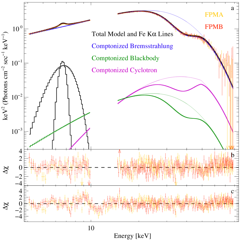
Figure 1: (a) Her X-1 4$-$79 keV X-ray unfolded (after Nowak et al. (2011)) spectrum from NuSTAR with residuals shown in the lower two panels. The two NuSTAR focal plane detectors are shown and the spectrum has been rebinned for clarity (see text). The final reduced $\chi^{2}$ is 1.212 for 450 degrees of freedom. The individual Comptonized emission components are shown. The dotted lines represent the Comptonized components with the multiplicative effects of cyclotron absorption removed. The model is dominated by Comptonized bremsstrahlung emission as suggested by BW. Close examination of the Comptonized cyclotron component reveals a mild discontinuity that results from the monochromatic injection of cyclotron photons at the local cyclotron energy at the neutron star surface (49.3 keV). (b) The top set of residuals are from our best fit [panel (a)] with the 10$-$14.5 keV region of the spectrum removed (see text) and all the two Fe emission line parameters free to vary. (c) The bottom residuals are from our best fit to the full energy range 4$-$79 keV and with the Fe-line widths fixed at the values obtained by Fürst et al. (2013). The small systematic deviations in the 9$-$14 keV range are most likely due to uncalibrated effects from the Tungsten coating on the NuSTAR mirrors.

4 Results

We performed our spectral fit in the XSPEC v12.8.2 and 12.9.0 (Arnaud, 1996) spectral analysis environments. We verified that the resulting fits are consistent across both versions of XSPEC. 23 parameters describe the spectral continuum and emission lines that NuSTAR observes in the 4 to 79 keV range. Six parameters describe two iron emission lines (we use the gaussian function for both lines), three describe the cyclotron resonant scattering absorption feature (CRSF), one parameter describes the interstellar absorption ($N_{\mathrm{H}}$), and one parameter describes the cross-normalization of the FPMA and FPMB modules (C_FPM). The absorbing column is frozen at $N_{\mathrm{H}}\,=\,1.7\times 10^{20}$ cm^-2, a value that approximates the galactic absorption to Her X-1 (Fürst et al., 2013). We utilized the tbabs absorption model with the “WILM” abundance table and the “BCMC” cross sections (Wilms et al., 2000). This leaves 12 parameters to describe the RDRS model. One of these is a RDRS model normalization that we freeze at 1.0. One is a numerical switch that allows us to turn on or off any of the three principal seed photon processes for the Comptonization (see Section 2). We freeze the distance to the Her X-1 system at $D=6.6$ kpc (Reynolds et al., 1997), and the NS mass and radius are set to their standard values ($1.4\,\,M_{\odot}$ and $10$ km). The distance to Her X-1 obtained by Reynolds et al. of $6.6_{-0.4}^{+0.4}$ kpc is sufficiently consistent, for our purposes, with a more recently determined distance of $6.1_{-0.4}^{+1.0}$ kpc obtained by Leahy & Abdallah (2014). Thus, we adopt the Reynolds et al. distance for these calculations. The value of the input magnetic field strength to the RDRS model is tied to the centroid of the fitted cyclotron absorption line ($E_{\mathrm{CRSF}}$) via $B/(10^{12}\mathrm{Gauss})\,=B_{12}\,=\,(1+z_{*})E_{\mathrm{CRSF}}/11.57$ where $z_{*}$ is the gravitational redshift to the NS surface. The six remaining parameters describing the RDRS model (BW) are: mass accretion rate ($\dot{M}$), plasma Comptonizing temperature ($T_{e}$), accretion cap radius ($r_{0}$), scattering cross section perpendicular to the magnetic field ($\sigma_{\perp}$), scattering cross section parallel to the magnetic field ($\sigma_{\parallel}$), and average scattering cross section ($\bar{\sigma}$). The scattering cross section perpendicular to the magnetic field ($\sigma_{\perp}$) is frozen at the Thomson electron scattering cross section ($\sigma_{\mathrm{T}}$). This leaves five free parameters, $\dot{M}$, $T_{e}$, $r_{0}$, $\sigma_{\parallel}$, and $\bar{\sigma}$, to describe the X-ray continuum.

The fit to the observed NuSTAR spectrum of Her X-1 is shown in Figure 1. Initially, we tried to fit the full energy range of 4 to 79 keV to the calculated radiation-dominated shock spectrum. However, in the resulting fit, the broad iron line component (FeK$\alpha_{\rm b}$) significantly modifies the continuum in the range below 15 keV. This broad iron feature apparently smooths deviations of the observed spectrum from the computed model in the 8$-$15 keV range. A similar difficulty was encountered by Fürst et al. (2013) in this same spectral region. To test for this possibility, we fixed the two iron line widths at the values found by Fürst et al. (2013). As a result of this, just as found by Fürst et al., the observed spectrum in the energy range of 9$-$15 keV has systematic residuals in comparison with the computed model spectrum. The reduced $\chi^{2}$ value is 1.42 for 500 degrees of freedom and the model residuals are shown in the bottom panel in Figure 1. These systematic residuals are most likely caused by imperfections in the response matrices due to Tungsten the edges from 8.39 to 12.10 keV induced by the X-ray mirror coatings (Madsen et al., 2015). Following the procedure of Fürst et al. (2013), we removed the spectral points in the energy range 10$-$14.5 keV. The fit is now significantly better with reduced $\chi^{2}$ of 1.212 for 450 degrees of freedom which is as good as any of the empirical fits obtained by Fürst et al. (2013). The best-fit parameters are given in Table 1 along with their formal 90% confidence errors. The continuum fit with the radiation-dominated shock model conforms very well to the observed background subtracted Her X- 1 spectrum. Examination of the contributions to $\chi^{2}$ as a function of energy suggest that there are still some deviations at the highest energies in our spectral range (65$-$79 keV). This is most likely because the background spectrum becomes as large or larger than the Her X-1 source spectrum above about 65 keV.

4.1 Accretion Rate

The accretion rate is ultimately determined by requiring that the total luminosity $L_{\rm X}$ in the three Comptonized spectral components (bremsstrahlung, cyclotron, and blackbody emission) integrated over the range 0.1-100 keV is equal to the Her X-1 accretion luminosity ($L_{\mathrm{acc}}\,=\,GM_{*}\dot{M}/R_{*}$). We also require that the observed flux in the 5$-$75 keV band equals the model flux in this same energy band. This leads to the need to iterate on the mass accretion rate ($\dot{M}$) by first estimating the accretion rate based on an approximate luminosity and then refining that estimate as one fits a series of models to the data until both of these conditions are satisfied for one set of model parameters. One source of uncertainty in the accretion rate is the uncertainty in the distance to Her X-1. There is also the possibility of some thermal energy being transported into the star at the base of the column (e.g., Basko & Sunyaev, 1976). If energy is transported into the star, then it would obviously create an offset between the values of $L_{\rm acc}$ and $L_{\rm X}$. In the absence of a comprehensive model that treats both the stellar surface and the shocked emitting region, it is not possible to specify the exact surface boundary condition. BW assumed that the radiated energy vanishes at the stellar surface, and we adopt the BW surface boundary condition in our work, by setting $L_{\rm X}=L_{\mathrm{acc}}=GM_{*}\dot{M}/R_{*}$, where the value of $L_{\rm X}$ is set equal to the luminosity emitted in the energy range 0.1$-$100 keV. In Section 4.6, we discuss the results obtained for the model parameters by artificially varying $\dot{M}$ around the value computed by setting $L_{\rm X}=L_{\rm acc}$.

4.2 Model Parameters

In general, the parameters from our fit are not too different from the approximate parameters obtained by BW for Her X-1. BW found the spectral shape was approximated sufficiently well in their low resolution limit by $r_{0}\,=\,44$ m whereas we obtain $r_{0}\,=\,107.0^{+1.7}_{-1.8}$ m, and BW found the column to be somewhat hotter at $kT_{e}\sim 5.4$ keV, compared to our fitted $kT_{e}\sim 4.58^{+0.07}_{-0.08}$ keV. The temperature we find for the thermal mound in our model is only a little below this at 3.8 keV. This temperature is about twice the Eddington temperature for the NS surface of $\sim 1.9$ keV. This is reasonable because blackbody photons are Compton scattered in the hot plasma, re-directing them out the sides of the column. This reduces the ability of those photons to halt the accretion flow by exchanging outward directed momentum with the falling electrons. Finally, note that this thermal mound temperature is significantly lower than the effective temperature of $\sim 9.1$ keV predicted by Mushtukov et al. (2015) in the disk accretion case for our model parameters with $\Lambda\sim 0.5$.

At an estimated distance of 6.6 kpc (Reynolds et al., 1997), based on the fitted model parameters, for this observation the 0.1$-$100 keV luminosity of Her X-1 is about $4.9\times 10^{37}$ ergs s^-1 and we expect this accretion flow to be radiation-dominated near the NS surface. As found by BW, Comptonized bremsstrahlung photons constitute the bulk of the observed emission in hard X-rays and Comptonized cyclotron and thermal mound blackbody photons are not significant contributors. Our model fit conforms to the expectation (see BW) for the resulting mean scattering cross sections in that we do indeed find that $\sigma_{\parallel}\,<\,\bar{\sigma}\,<\,\sigma_{\perp}$. When we compare the flux we derive from the fit in the 5$-$60 keV energy range with that of Fürst et al. (2013), we find after accounting for the new calibration released in October 2013, our 5$-$60 keV flux agrees with the Fürst et al. flux within 2%. When we compare our derived value of $\xi\sim 1.355$ with the value $\xi$ should have in a pure radiation-dominated shock ($\xi\sim 1.15$) (see BW) we are about 18% high which we believe is an indication of the divergence of our assumed “hot slab” structure with approximate velocity law to a full radiation-hydrodynamic solution in which the plasma comes to rest at the NS surface. Comparing our result to the approximate result of BW, we obtain $\delta\sim 2.38$, which is still a moderate value. For this $\delta$-value equation (3) yields $y_{\rm bulk}\sim 0.59\,\,y_{\rm thermal}$ which indicates that in our formulation, bulk Comptonization is slightly less important than thermal Comptonization in determining the overall Her X-1 X-ray spectral shape. That thermal Comptonization is important is shown by the fact that the Her X-1 spectrum is relatively flat at intermediate energies and turns over above 30 keV. However, thermal Comptonization is not so strong (i.e., saturated) in our model that a Wien peak is formed in the spectrum.

4.3 Iron Emission

We model the iron line complex as consisting of a narrow line at $\sim$6.6 keV (the “n” subscript) and a broad line at the lower energy of $\sim$6.5 keV (the “b” subscript). This is similar to the iron line model of Fürst et al. (2013) We have also removed the range 10$-$14.5 keV as did Fürst et al. As we noted above retaining this region would have the effect of broadening one of the Fe-lines to “smooth over” some of the calibration residuals in this energy range so we delete this section of the energy spectrum. Furthermore, we only fit the NuSTAR X-ray spectrum here while Fürst et al. fit the combined spectra from NuSTAR and Suzaku in the region below 10 keV and Suzaku had higher spectral resolution than NuSTAR. Fürst et al. fit a number of different continuum models and we compare our fit to their “HighE” cutoff power law model from their Table 3. For the “narrow” iron line, Fürst et al. (2013) found an energy centroid of $E({\rm FeK}\alpha_{\rm n})=6.601^{+0.017}_{-0.016}$ keV and $\sigma({\rm FeK}\alpha_{\rm n})=0.25^{+0.04}_{-0.04}$ keV which agree within the errors of the values we find for $E({\rm FeK}\alpha_{\rm n})=6.61^{+0.02}_{-0.02}$ keV and $\sigma({\rm FeK}\alpha_{\rm n})=0.26^{+0.03}_{-0.04}$ keV. Thus, the narrow Fe-line fits are essentially consistent within the uncertainties. For the “broad” iron line we obtain an energy centroid of $E({\rm FeK}\alpha_{\rm b})=6.53^{+0.07}_{-0.08}$ keV and $\sigma({\rm FeK}\alpha_{\rm b})=0.90^{+0.21}_{-0.14}$ keV whereas Fürst et al. find $E({\rm FeK}\alpha_{\rm b})=6.55^{+0.05}_{-0.05}$ keV and $\sigma({\rm FeK}\alpha_{\rm b})=0.82^{+0.13}_{-0.10}$ keV. Again, our broad line agrees within the errors with the line parameters found by Fürst et al. Asami et al. (2014) found in their analysis of Suzaku data alone from Her X-1 that their spectral fits required a broad line in the 4$-$9 keV energy range. They suggested a number of possible physical origins for this feature but their data was not sufficient to attribute the line emission to one unique mechanism. The iron line signatures in the 4$-$9 keV range of the spectrum is complex with perhaps more than one narrower line sitting on top of a broad continuum consisting of many line components that are not yet full resolved by either of these instruments.

4.4 Scattering Cross Sections and Cyclotron Absorption

We included a CRSF absorption line with the gabs multiplicative model component in our broad band fit. The energy centroid of our fit is $E_{\mathrm{CRSF}}=37.7_{-0.2}^{+0.2}$ keV, which falls within the error range of the value obtained by Fürst et al. (2013), $E_{\mathrm{CRSF}}=37.40_{-0.24}^{+0.25}$ keV. However, our line width, $\sigma_{\mathrm{CRSF}}=7.1_{-0.2}^{+0.2}$ keV, is somewhat larger than the Fürst et al. result of $\sigma_{\mathrm{CRSF}}=5.76_{-0.27}^{+0.29}$ keV. The cyclotron resonant scattering feature absorption line optical depth can be written as $\tau_{\mathrm{CRSF}}={\rm Strength}/(\sigma_{\mathrm{CRSF}}\sqrt{2\pi})$. In our fit $\tau_{\mathrm{CRSF}}\sim 0.98_{-0.06}^{+0.06}$ whereas Fürst et al. obtain $\tau_{\mathrm{CRSF}}\,\sim\,0.614_{-0.025}^{+0.028}$. Thus, our CRSF absorption line is deeper than the line found by Fürst et al. This is not a large difference and may result from our different continuum model.

BW froze the perpendicular scattering cross section to the Thomson value ($\sigma_{\perp}\equiv\sigma_{\rm T}$) in their analytical model and we adopt this approximation here. However, this approximation does warrant further discussion. Below the cyclotron resonant energy, the cross section of ordinary polarization mode photons (i.e., photons with electric field vectors in the plane formed by the pulsar magnetic field and the photon propagation direction) will be roughly constant with energy at the Thomson value. The extraordinary mode photons (i.e., those photons with electric field vectors oriented perpendicular to the plane formed by the pulsar magnetic field and the photon propagation direction) have a scattering cross section significantly below Thomson at energies below $\epsilon_{c}$ because in this range the extraordinary mode scattering cross section varies as $\sigma_{\rm ext}\propto(\epsilon/\epsilon_{c})^{2}$ (see Nagel, 1981). Utilizing a simple slab geometry with a numerical formulation of the transport equation, Nagel was able to show that at high Thomson scattering optical depths the emerging X-ray spectrum in the energy range $<20$ keV could be dominated by extraordinary mode photon emission. We are working in a parameter regime where the perpendicular Thomson scattering optical depth is $\tau_{\perp}\,\sim\,t_{\rm esc}c/r_{0}\sim 1100$ according the BW Equation (17) and thus large. Hence, the spectra of Her X-1 below the first cyclotron resonance may be dominated by extraordinary mode photon emission.

Furthermore, in Her X-1 we also see that most of the emergent radiated energy comes out near the cyclotron energy and thus setting the perpendicular cross section to Thomson is not an unreasonable approximation. We therefore model the electron scattering of both modes perpendicular to the magnetic field as occurring at the Thomson rate. Furthermore, the extraordinary mode photons interact most strongly with electrons at the resonance energy via absorption, which is followed almost immediately by the emission of a cyclotron photon at the same energy but in a different direction. In the frame of the neutron star, this is essentially a resonant elastic scattering (see Nagel, 1980). The net effect of this resonant scattering process is negligible within the context of our model, since our transport equation is angle-averaged. Therefore, the appropriate way to include this effect in our spectral modeling is to impose an absorption feature as part of the XSPEC modeling of the emergent spectrum, which is what we do. More detailed future calculations of the X-ray spectra of high luminosity accreting X-ray pulsars are needed to explore this issue.

In our model, we implicitly assume that the cyclotron absorption feature is associated with the same magnetic field value as the cyclotron emission. However, in principle, one may consider the possibility of “disconnecting” the cyclotron emission magnetic field from the cyclotron absorption magnetic field, if one supposes that emission occurs primary in a separate region of the accretion column from the location where the cyclotron scattering feature is imprinted (e.g., see Ferrigno et al., 2009). This is a further level of approximation when cast within the context of a cylindrical model that doesn’t include a self-consistent calculation of the electron temperature or the velocity profile. Moreover, in the particular application to Her X-1 made in this paper, the distinction between the two fields will make no difference for the model fits, since the contribution to the observed spectrum from the Comptonized cyclotron component is negligible. In the future, the actual dipole variation of the field should be included, along with the flow dynamics and the variation of the electron temperature (see discussion in Section 4.6).

4.5 Relation to Previous Work

Ferrigno et al. (2009) were the first to implement computationally a version of the BW formalism, with a specific application to the analysis of 4U 0115$+$63. 4U 0115$+$63 has a magnetic field strength of $\sim 10^{12}$ G resulting in cyclotron photons being a very significant seed photon source for Comptonization in the accreting plasma near the NS surface. Furthermore, the fundamental CRSF and as many as four harmonics have been detected in this source (Ferrigno et al., 2009). In their modeling of the X-ray spectrum, Ferrigno et al. concluded that the BW Comptonization model can account for the X-ray spectral continuum above $\sim$9 keV as resulting from Comptonized cyclotron photons. In order to obtain a reasonable spectral fit below 9 keV, Ferrigno et al. found that an additional power law component, possibly resulting from Comptonized blackbody photons emerging from a significant fraction of the NS surface, was required. The work of Ferrigno et al. also included an attempt to implement phase-resolved spectroscopy, although their application of the column-integrated BW model meant that the phase-resolved fits should really be interpreted as rough estimates, since they allowed the BW model parameters to vary as a function of the star’s spin phase, rather than employing a single fixed model for the column, and allowing it to be viewed from various observation angles. This latter scenario, while more accurate, cannot be implemented without the availability of a height-dependent version of the BW model (rather than the column-averaged formulation), and no such analytical model has appeared yet. The phase-dependent calculations of Ferrigno et al. (2009) did not include a specific geometrical model for the location of the accreting magnetic pole relative to the spin axis, nor any treatment of general relativistic effects in the strong gravitational field.

Subsequent papers by Farinelli et al. (2012) and Farinelli et al. (2016) presented a more detailed approach. Farinelli et al. (2012) adopted the overall BW formulation of the transport equation but added an additional term to the stochastic part of the transport equation intended to account for the effects of the bulk motion of the electrons, and these authors also implemented a more general power law velocity profile, in addition to the simple velocity law given by Equation (2). However, the seed photons in the Farinelli et al. case were blackbody distributed across the column with an exponential dependence on height. The additional model terms are not a part of the original BW model, and as such, the Farinelli et al. study is not an exact implementation of the BW model. The inclusion of the additional terms renders the transport equation unsolvable using analytical methods, and therefore the authors obtain a series of numerical solutions. Farinelli et al. (2016) further enhanced this treatment by including a distributed bremsstrahlung and cyclotron seed photon source for the Comptonization process. Furthermore, Farinelli et al. (2016) introduced the vertical dependency of the magnetic field emission in their cyclotron seed photon source term. Moreover, both Farinelli et al. (2012) and Farinelli et al. (2016) fix the average scattering cross sections to $\sigma_{\parallel}=10^{-3}\sigma_{\rm T}$ and $\bar{\sigma}=10^{-1}\sigma_{\rm T}$, and therefore the remaining model parameters, such as the polar cap radius ($r_{0}$) and the Comptonizing temperature ($kT_{e}$), are not easy to compare to our fitted values. The Farinelli et al. (2016) treatment was utilized to fit the phase-averaged spectral data for the three sources Her X-1, 4U 0115$+$63, and Cen X-3.

Each of the previous models discussed above is an important contribution in its own right, and they are all offshoots of the original BW model. However, each of these models is unable to account for three important issues that may have a significant effect on the emergent spectra in accretion-powered X-ray pulsars. The first issue is the importance of utilizing a self-consistent velocity profile in the accretion column. This is a central concern, because the velocity field in luminous X-ray pulsars is mediated mainly by the radiation pressure, which decelerates the flow to rest at the stellar surface. But because the radiation pressure profile depends on the velocity field through the transport equation, ideally, the velocity field calculation should be accomplished in a self-consistent manner. The self-consistent calculation requires the utilization of a sophisticated, iterative algorithm that is beyond the realm of implementation in XSPEC. The second issue is that none of the cited models utilizes a realistic energy equation to determine the vertical variation of the electron temperature in the column, instead assuming (as we do) that the electrons are isothermal. Again, a self-consistent calculation of the thermal structure of the column is difficult to include in an XSPEC module. Finally, the third issue is the implementation of a cylindrical geometry for the accretion column, and a constant magnetic field, which is probably acceptable for “pill-box” situations, but may lead to unknown errors in sources where the column has a significant vertical extent, compared with the radius of the star. The lack of self-consistency in the treatment of the hydrodynamics, the electron temperature, and the accretion geometry clearly introduces errors that are very difficult to estimate with precision.

4.6 Model Limitations and Uncertainties

The BW model assumes that all of the emergent radiation escapes through the sides of the magnetic funnel in a fan beam, rather than out of the top of the shocked plasma region in a pencil beam. Theoretical models available to-date do not settle the question of the predominance of either fan beam emission or pencil beam emission for accreting X-ray pulsars generally. However, some guidance can be obtained from observations. For example, Leahy (2004) performed a fit to fan and pencil beam components of the Her X-1 light curve in the 9$-$14 keV energy range during the main high state of the 35-day super-orbital period. For an assumed distance of 5 kpc, Leahy found that the best fit to the data yielded fan-beam and pencil-beam components with luminosities of $9.7\times 10^{35}$ ergs s^-1 and $1.4\times 10^{35}$ ergs s^-1, respectively, for one assumed pole. This is roughly a 7:1 ratio of fan emission vs. pencil emission. The energy range treated by Leahy is narrower than that we have considered above, and thus the Leahy luminosity will not match our observed luminosity. However, it does suggest that for Her X-1 at least, the assumption of fan-beam-only emission will not result in a large error.

The errors we give in Table 1 for the model input parameters result from the formal procedure of asking XSPEC to vary the likelihood statistic for each parameter to derive the 90% statistical error for each parameter in turn. However, in implementing the BW analytical model in XSPEC we have incorporated their assumption that a simple one-electron-temperature post-shock plasma emission region is an adequate approximation of a real flow. This results in our using the crude linear velocity relation to ensure that the flow stagnates at the NS surface. A real model must self-consistently solve for both the dynamical structure and the radiation transport simultaneously. Such models are in development but are not at the stage where they can be implemented in XSPEC (see West et al. 2016, submitted). The development of numerical models will also help to answer the questions regarding the height-dependent seed photon injection rates we now discuss.

The height of the sonic point $z_{\rm sp}$ above the NS can be estimated from BW Equation (31) while the value of $z_{\rm max}$ from BW Equation (80) determines the extent of the spatial integration of the injected seed photon distribution within the accretion column in our model (see Equation (126) of BW). For the fitted model shown in Table 1, we find $z_{\rm sp}=3.63$ km and $z_{\rm max}=6.67$ km, and hence the sonic point is located within the seed-photon integration region as it should be. The corresponding model optical depth for $z_{\rm max}$ we find from BW Equation (79) is 1.33, which compares very favorably with the value of 1.37 found originally by BW (see Table 2 of BW).

When we calculate the magnetic field “blooming” for the dipole geometry from the NS surface to $z_{\rm sp}$ we find that $((R_{\rm NS}+z_{\rm sp})/R_{\rm NS})^{3}\sim 2.5$ suggesting that our assumption of cylindrical geometry is not very accurate. Furthermore, the derived magnetic field strength is reduced from $B_{12}=4.25$ at the NS surface to $B_{12}=1.68$ at the height $z_{\rm sp}$ above the NS surface. However, this effect is somewhat mitigated by the fact that cyclotron excitation (and therefore the resulting spontaneous emission) is concentrated in the dense lower region of the column below $z_{\rm sp}$. The assumption of cylindrical geometry is not likely to strongly distort the results relative to a dipole geometry since most of the radiation escapes through the column walls in the lower region of the column, in the vicinity of the sonic point for the standing, radiation-dominated shock wave (Becker, 1998).

We can understand this by noting that the number of seed photons injected via cyclotron decays varies as ${\dot{n}}^{\rm cyc}_{\epsilon}\propto\rho^{2}B_{12}^{-3/2}$ (Arons et al., 1987). This reflects the fact that excitation to the first Landau level for the electrons is a two-body process, and also that as the magnetic field strength goes up it becomes more difficult for collisions to supply the energy needed to excite electrons from the ground state to the first Landau level. At the top of the accretion column ($z=z_{\rm max}$), the local magnetic field strength is lower than the nominal value associated with the CRSF, which reduces the energy spacing between the ground state and the first Landau level making electron excitation easier to accomplish. However, this is offset by the relatively low value of the plasma density at $z_{\rm max}$, where the flow velocity is roughly half the speed of light. These two effects combine to produce a low value of the cyclotron seed photon production rate ${\dot{n}}^{\rm cyc}_{\epsilon}$ at the top of the column. Further down in the column, the magnetic field strength is higher, and this makes collisional excitation more difficult. However, this difficulty is overwhelmed by the rapidly increasing density as the flow is decelerated. Utilizing our rough velocity parameterization and assuming dipolar field geometry we find that for our Her X-1 model, ${\dot{n}}^{\rm cyc}_{\epsilon}$ is strongly peaked at altitudes below $z_{\rm sp}$. As we noted above we incorporate the BW assumption that the cyclotron seed photon production rate is determined by the value of the magnetic field strength that is input to the model based on the fitted energy centroid of the gaussian CRSF, and the effects of Landau level collisional de-excitation are not included. Future models will need to address how to optimally account for the variation in the magnetic dipolar accretion geometry and the varying density throughout the column.

Another source of possible error is that we do not include the effects of general relativity (GR) in our model. GR would redshift the observed luminosity of the accretion flow compared to its value at the NS surface and thus increase the derived mass accretion rate (at the NS surface) for a given observed luminosity. For our standard NS parameters the red shift at the NS surface is roughly $z_{*}\sim 0.3$. However, for emission further up the column the apparent red shift would be reduced for emission originating well above the NS surface. Thus, it is not as simple as just multiplying luminosities and mass accretion rates by factors of $(1+z_{*})^{2}$ and $(1+z_{*})^{-2}$, respectively. As a pole spins into and out of view that portion of its emission that is bent around the NS and reaches the observer will vary with phase. We reiterate that the value for the mass accretion rate we derive here is based on full energy conservation (i.e., assuming 100% efficiency in converting flow gravitational potential into radiated energy), which is necessary in order to maintain consistency with the surface boundary condition (zero energy flux) assumed by the BW model.

Another source of error in the application of these calculations stems from the ambiguity in determining if one pole or two poles are actually accreting simultaneously in the modeled system. If only one pole on the star is accreting, then the parameters we derive in our fit to the NuSTAR spectrum should be a relatively accurate reflection of the real conditions at that pole. If, on the other hand, there are two accreting poles, then what we observe from Her X-1 is only the phase-averaged luminosity and we cannot discern how that luminosity is apportioned between these two poles (assuming a dipolar field) using our model. Furthermore, the apparent flux coming from each pole is a function of spin phase. All we can really say is that if the accretion flow onto the NS is substantially divided between two poles, then we expect that emission from each pole will result from a shock structure that reflects a lower accretion rate than the one we adopt here. In summary, we can say that the mean accretion rate onto the NS is no lower than our fitted rate but we cannot say how that accreting material is divided between the accretion poles.

This suggests it would be useful to determine if the character of the solutions might change if we relax our energy conservation demand and perturb the accretion rate. Thus, we fit models to the NuSTAR data in which we arbitrarily change the accretion rate by $\pm$30% (to $\dot{M}=1.82\times 10^{17}\,{\rm g}\,{\rm s}^{-1}$ and $\dot{M}=3.37\times 10^{17}\,{\rm g}\,{\rm s}^{-1}$, respectively) and only demand that the flux in the 5$-$75 keV band is correctly accounted for during the fits. The fit statistics are similar to our base model (see Table 1) in that $\chi^{2}/{\rm DoF}=549.41/450$ (-30%) and $\chi^{2}/{\rm DoF}=544.77/450$ (+30%) so the quality of these fits are all similiar. We find that the polar cap radius and the scattering cross sections do noticeably change, but other fitted parameters, such as the Comptonizing temperature, do not change significantly. For example, the accretion cap radius changed from $\sim$107 m with our base model accretion rate ($\dot{M}=2.59\times 10^{17}\,{\rm g}\,{\rm s}^{-1}$, see Table 1) to $\sim$57 m at the reduced rate and $\sim$167 m at the increased rate. This illustrates that the radius of the accreting pulsar cap is a strong function of the accretion rate in the BW model. Moreover, the mean scattering cross section changed from $\sim 3.5\times 10^{-4}\sigma_{\mathrm{T}}$ for our base model to $\sim 1.9\times 10^{-4}\sigma_{\mathrm{T}}$ at the reduced rate and $\sim 5.3\times 10^{-4}\sigma_{\mathrm{T}}$ at the increased rate. However, the Comptonizing temperature ($kT_{e}$) changed by less than 3% in either direction with the variation of the accretion rate. This means that the accretion rate changes maintained the basic shock structure as radiation-dominated with $(\xi,\delta)\sim(1.30,2.33)$ and $(\xi,\delta)\sim(1.38,1.91)$ for the low and high accretion rates, respectively, whereas $(\xi,\delta)\sim(1.36,2.38)$ for our base accretion rate. Thus, the models with the perturbed accretion rates are still dominated by thermal Comptonization over bulk Comptonization by roughly a factor of 2.

5 Conclusions

We describe improved spectral modeling of the accreting X-ray pulsar Hercules X-1 with a radiation-dominated radiative shock model, based on the analytic work of BW. We perform a detailed quantitative spectral fit in XSPEC using a physics-based BW model intended for general release. This results in estimates for the accretion rate, the Comptonizing temperature of the post-shock radiating plasma in the accretion column as it hits the NS surface, the radius of the accretion column, the mean scattering cross section parallel to the magnetic field, and the flow overall angle-averaged scattering cross section that regulates the thermal Comptonization process. We obtain a good fit to the spin-phase averaged 4 to 78 keV X-ray spectrum observed by NuSTAR during a main-on of the Her X-1 35-day accretion disk precession period over the entire energy range of the observation with our radiation-dominated radiative accretion shock model. This demonstrates the utility of the BW radiation-dominated radiative shock model implementation in constraining the real physical parameters of high luminosity accreting X-ray pulsar sources.

Table 1: Her X-1 XSPEC Model Parameters

Parameter	Value
$N_{\mathrm{H}}$ (cm-2)	$1.7\times 10^{20}$ (Fixed)
Distance (kpc)	6.6 (Fixed)
$\dot{M}$ (g s-1)	$2.5935\times 10^{17}$ (Fixed)
$kT_{e}$ (keV)	$4.58_{-0.07}^{+0.07}$
$r_{0}$ (m)	$107.0_{-1.8}^{+1.7}$
$B$ (Gauss)	$4.25\times 10^{12}$ (Tied to $E_{\rm CRSF}$)
$\sigma_{\perp}$ ($\sigma_{\mathrm{T}}$)	1.0 (Fixed)
$\sigma_{\parallel}$ ($\sigma_{\mathrm{T}}$)	$5.20_{-0.07}^{+0.08}\times 10^{-5}$
$\bar{\sigma}$ ($\sigma_{\mathrm{T}}$)	$3.5_{-0.2}^{+0.2}\times 10^{-4}$
$E_{\mathrm{CRSF}}$ (keV)	$37.7_{-0.2}^{+0.2}$
$\sigma_{\mathrm{CRSF}}$ (keV)	$7.1_{-0.2}^{+0.2}$
$\tau_{\mathrm{CRSF}}$	$0.98_{-0.06}^{+0.06}$
$E({\rm FeK}\alpha_{\rm n})$ (keV)	$6.61_{-0.02}^{+0.02}$
$\sigma({\rm FeK}\alpha_{\rm n})$ (keV)	$0.26_{-0.04}^{+0.03}$
$\rm A({\rm FeK}\alpha_{\rm n})$	$0.0029_{-0.0006}^{+0.0006}$
$E({\rm FeK}\alpha_{\rm b})$ (keV)	$6.53_{-0.08}^{+0.07}$
$\sigma({\rm FeK}\alpha_{\rm b})$ (keV)	$0.90_{-0.14}^{+0.21}$
$\rm A({\rm FeK}\alpha_{\rm b})$	$0.0043_{-0.0005}^{+0.0005}$
CFPM	$1.037_{-0.002}^{+0.002}$
$\chi^{2}/{\rm DoF}$	$545.55/450$
$\rm Flux(5-60\,{\rm keV})$ (ergs ${\rm cm}^{-2}$ ${\rm s}^{-1}$)	$6.96_{-0.01}^{+0.01}\times 10^{-9}$

References

- Abramowitz & Stegun (1970) Abramowitz, M., & Stegun, I. A. 1970, Handbook of Mathematical Functions (NY, Dover)
- Arnaud (1996) Arnaud, K. A. 1996, in AIP Conference Series, Vol. 101, Astronomical Data Analysis Software and Systems V, ed. G. H. Jacoby & J. Barnes, 17
- Arons et al. (1987) Arons, J., Klein, R. I., & Lea, S. M. 1987, ApJ, 312, 666
- Asami et al. (2014) Asami, F., et al. 2014, PASJ, 66, 44
- Bachetti et al. (2014) Bachetti, M., et al. 2014, Nature, 514, 202
- Basko & Sunyaev (1975) Basko, N. M., & Sunyaev, R. A. 1975, Sov. Phys. JETP, 41, 52
- Basko & Sunyaev (1976) Basko, N. M., & Sunyaev, R. A. 1976, MNRAS, 175, 395
- Becker (1998) Becker, P. A. 1998, ApJ, 498, 790
- Becker & Wolff (2007) Becker, P. A., & Wolff, M. T. 2007, ApJ, 654, 435
- Becker et al. (2012) Becker, P. A., et al. 2012, A&A, 544, A123
- Boldin et al. (2013) Boldin, P. A., Tsygankov, S. S., & Lutovinov, A. A. 2013, Astronomy Letters, 39, 375
- Davidson & Ostriker (1973) Davidson, K., & Ostriker, J. P. 1973, ApJ, 179, 585
- di Salvo et al. (1998) di Salvo, T., et al. 1998, ApJ, 509, 897
- Farinelli et al. (2012) Farinelli, R., et al. 2012, A&A, 538, A67
- Farinelli et al. (2016) Farinelli, R., et al. 2016, ArXiv e-prints
- Ferrigno et al. (2009) Ferrigno, C., et al. 2009, A&A, 498, 825
- Fürst et al. (2013) Fürst, F., et al. 2013, ApJ, 779, 69
- Harding et al. (1984) Harding, A. K., et al. 1984, ApJ, 278, 369
- Harrison et al. (2013) Harrison, F. A., et al. 2013, ApJ, 770, 103
- Klein et al. (1996) Klein, R. I., et al. 1996, ApJ, 457, L85+
- Langer & Rappaport (1982) Langer, S. H., & Rappaport, S. 1982, ApJ, 257, 733
- Leahy (2004) Leahy, D. A. 2004, ApJ, 613, 517
- Leahy & Abdallah (2014) Leahy, D. A., & Abdallah, M. H. 2014, ApJ, 793, 79
- Levine et al. (1991) Levine, A., et al. 1991, ApJ, 381, 101
- Lyubarskii & Syunyaev (1982) Lyubarskii, Y. E., & Syunyaev, R. A. 1982, Soviet Astronomy Letters, 8, 330
- Madsen et al. (2015) Madsen, K. K., et al. 2015, ApJS, 220, 8
- Mészáros & Nagel (1985) Mészáros, P., & Nagel, W. 1985, ApJ, 298, 147
- Müller et al. (2013) Müller, S., et al. 2013, A&A, 551, A6
- Mushtukov et al. (2015) Mushtukov, A. A., et al. 2015, MNRAS, 447, 1847
- Nagel (1980) Nagel, W. 1980, ApJ, 236, 904
- Nagel (1981) Nagel, W. 1981, ApJ, 251, 288
- Nelson et al. (1993) Nelson, R. W., Salpeter, E. E., & Wasserman, I. 1993, ApJ, 418, 874
- Nowak et al. (2011) Nowak, M. A., et al. 2011, ApJ, 728, 13
- Reynolds et al. (1997) Reynolds, A. P., et al. 1997, MNRAS, 288, 43
- Rybicki & Lightman (1979) Rybicki, G. B., & Lightman, A. P. 1979, Radiative Processes in Astrophysics (John Wiley & Sons: New York)
- Scott & Leahy (1999) Scott, D. M., & Leahy, D. A. 1999, ApJ, 510, 974
- Staubert et al. (2007) Staubert, R., et al. 2007, A&A, 465, L25
- Tsygankov et al. (2010) Tsygankov, S. S., Lutovinov, A. A., & Serber, A. V. 2010, MNRAS, 401, 1628
- Vasco et al. (2011) Vasco, D., Klochkov, D., & Staubert, R. 2011, A&A, 532, A99
- Wilms et al. (2000) Wilms, J., Allen, A., & McCray, R. 2000, ApJ, 542, 914