Detection relic gravitational waves in thermal case by using Adv.LIGO data of GW150914

Abstract

The thermal spectrum of relic gravitational waves causes the new amplitude that called ‘modified amplitude’. Our analysis shows that, there exist some chances for detection of the thermal spectrum in addition to the usual spectrum by using Adv.LIGO data of GW150914 and detector based on the maser light(Dml). The behaviour of the inflation and reheating stages are often known as power law expansion like $S(\eta)\propto\eta^{1+\beta}$, $S(\eta)\propto\eta^{1+\beta_{s}}$ respectively. The $\beta$ and $\beta_{s}$ have an unique effect on the shape of the spectrum. We find some upper bounds on the $\beta$ and $\beta_{s}$ by comparison the usual and thermal spectrum with the Adv.LIGO and Dml. As this result modifies our information about the nature of the evolution of inflation and reheating stages.

I Introduction

The relic gravitational waves (RGWs) have a wide range of frequency $\sim($10^-19Hz -10¹¹Hz). They are generated before and during inflation stage. They did not have interaction with other matters during their travel from the early universe until now. Therefore they contain valuable information about the early universe. Thus we can obtain the information by detecting RGWs on the through range of the frequency. Nowadays the people are trying to detect the waves at different frequency ranges like: $\sim($10^-19Hz -10^-16Hz) by Planck 1 , $\sim($10^-7Hz -10⁰Hz) by eLISA 2 , $\sim($10^-1Hz -10⁴Hz) by Advanced.LIGO (Adv.LIGO) 3 , $\sim($10⁰Hz -10⁴Hz) by Einstein telescope (ET) 4 , GHz band by detector based on the maser light (Dml)5 and etc. It is believed that thermal spectrum of RGWs exists from a pre-inflationary stage and it may affect on the CMB temperature and the polarization anisotropies in the low frequency range ($\sim$10^-18Hz-10^-16Hz) 6 . Then thermal spectrum of RGWs extend this investigation to the general pre-inflationary scenario by assuming the effective equation of state, $\omega$ being a free parameter 61 . Also in high frequency range $\sim($10⁸Hz -10¹¹Hz), extra dimensions cause thermal gravitational waves (or, equivalently, a primordial background of gravitons) 7 . For more details about the extra dimension see Ref.23 . For the gravity-wave background origin, any fit of the CMB anisotropy in term of gravity background should include a thermal dependence in the spectrum 71 . Thus in the middle range $\sim($10^-16Hz -10⁸Hz), this thermal spectrum causes the new amplitude that called ‘modified amplitude’ 8 . We have analysed the results of modified amplitude by comparison it with the sensitivity of the Adv.LIGO, ET and LISA in 8 . Recently Adv.LIGO has detected the effect of waves of a pair of black holes called GW150914 9 with a peak gravitational-wave strain of $1.0\times 10^{-21}$ in the frequency range 35 to 250 Hz. There is an average measured sensitivity in the range $\sim($10^-1Hz -10⁴Hz) of the Adv.LIGO detectors (Hanford and Livingston) during the time analysed to determine the significance of GW150914 (Sept 12 - Oct 20, 2015) 3 . Therefore in this work, we upgrade our previous work 8 by comparison the thermal spectrum with average measured sensitivity of Adv.LIGO and Dml. We show that there are some chances for detection the spectrum of RGWs in usual and thermal case.

On the other hand the different stages of the evolution of the universe (inflation, reheating, radiation, matter and acceleration) cause some variation in the shape of the spectrum of the RGWs. The behaviour of the inflation and reheating stages are often known as power law expansion like $S(\eta)\propto\eta^{1+\beta}$, $S(\eta)\propto\eta^{1+\beta_{s}}$ respectively. The $S$ and $\eta$ are scale factor and conformal time respectively and $\beta,\beta_{s}$ constrained on the $1+\beta<0$ and $1+\beta_{s}>0$ 11 ; 12 . The $\beta$ and $\beta_{s}$ have an unique effect on the shape of the spectrum in the full range $\sim($10^-19Hz -10¹¹Hz) and high frequency range $\sim($10⁸Hz -10¹¹Hz) respectively. Therefore these two parameters play main role in the spectrum of the RGWs. Thus, we are interested to obtain some upper bounds on the $\beta$ and $\beta_{s}$ by comparison the usual and thermal spectrum with the average measured sensitivity of the Adv.LIGO and Dml. As obtained result of the upper bounds can modify our information about the nature of the evolution of inflation and reheating stages. In the present work, we use the unit $c=\hbar=k_{B}=1$.

II The spectrum of gravitational waves

The perturbed metric for a homogeneous isotropic flat Friedmann-Robertson-Walker universe can be written as

$$ds^{2}=S^{2}(\eta)(d\eta^{2}-(\delta_{ij}+h_{ij})dx^{i}dx^{j}),$$ (1)

where $\delta_{ij}$ is the Kronecker delta symbol. The $h_{ij}$ are metric perturbations with the transverse-traceless properties i.e; $\nabla_{i}h^{ij}=0,\delta^{ij}h_{ij}=0$. The gravitational waves are described with the linearized field equation given by

$$\nabla_{\mu}\left(\sqrt{-g}\,\nabla^{\mu}h_{ij}(\bf{x},\eta)\right)=0.$$ (2)

The tensor perturbations have two independent physical degrees of freedom and are denote as $h^{+}$ and $h^{\times}$ that called polarization modes. We express $h^{+}$ and $h^{\times}$ in terms of the creation ($a^{\dagger}$) and annihilation ($a$) operators,

$$h_{ij}({\bf x},\eta)=\frac{\sqrt{16\pi}l_{pl}}{S(\eta)}\sum_{\bf{p}}\int\frac{d^{3}k}{(2\pi)^{3/2}}{\epsilon}_{ij}^{\bf{p}}(\bf{k})$$

$$\times\frac{1}{\sqrt{2k}}\Big{[}a_{\bf{k}}^{\bf{p}}h_{\bf{k}}^{\bf{p}}(\eta)e^{i\bf{k}.\bf{x}}+a^{\dagger}_{\bf{k}}{{}^{\bf{p}}}h^{*}_{\bf{k}}{{}^{\bf{p}}}(\eta)e^{-i\bf{k}.\bf{x}}\Big{]},$$ (3)

where $\bf{k}$ is the comoving wave number, $k=|\bf{k}|$, $l_{pl}=\sqrt{G}$ is the Planck’s length and $\bf{p}=+,\times$ are polarization modes. The polarization tensors $\epsilon_{ij}^{{\bf p}}({\bf k})$ are symmetric and transverse-traceless $k^{i}\epsilon_{ij}^{{\bf p}}({\bf k})=0,\delta^{ij}\epsilon_{ij}^{{\bf p}}({\bf k})=0$ and satisfy the conditions $\epsilon^{ij{\bf p}}({\bf k})\epsilon_{ij}^{{\bf p}^{\prime}}({\bf k})=2\delta_{{\bf p}{{\bf p}}^{\prime}}$ and $\epsilon^{{\bf p}}_{ij}({\bf-k})=\epsilon^{{\bf p}}_{ij}({\bf k})$. Also the creation and annihilation operators satisfy $[a_{{\bf k}}^{{\bf p}},a^{\dagger}_{{\bf k}^{\prime}}{{{}^{{\bf p}}}^{\prime}}]=\delta_{{{\bf p}}{\bf{p}}^{\prime}}\delta^{3}({\bf k}-{{\bf k}}^{\prime})$ and the initial vacuum state is defined as

$$a_{\bf{k}}^{\bf{p}}|0\rangle=0,$$ (4)

for each $\bf{k}$ and $\bf{p}$. For a fixed wave number $\bf{k}$ and a fixed polarization state $\bf{p}$ the eq.(2) gives coupled Klein-Gordon equation as follows:

$$f^{\prime\prime}_{k}+\Big{(}k^{2}-\frac{S^{\prime\prime}}{S}\Big{)}f_{k}=0.$$ (5)

where $h_{k}(\eta)=f_{k}(\eta)/S(\eta)$ 11 ; 12 and prime means derivative with respect to the conformal time. Since the polarization states are same, we consider $f_{k}(\eta)$ without the polarization index. The solution of the above equation for the different stages of the universe are given in appendix.[A]. There is another state that called ‘thermal vacuum state’ see appendix.[B] for more details. The amplitude of the RGWs in thermal vacuum state are as follows 8 :

$$h(k,\eta_{0})=A\Big{(}\frac{k}{k_{H}}\Big{)}^{2+\beta}\coth^{1/2}[\frac{k}{2T}],\;\;\;k\leq k_{E},$$ (6)

$$h(k,\eta_{0})=A\Big{(}\frac{k}{k_{H}}\Big{)}^{\beta-\gamma}(1+z_{E})^{\frac{-2-\gamma}{\gamma}}\coth^{1/2}[\frac{k}{2T}],\;\;\;k_{E}\leq k\leq k_{H},$$ (7)

$$h(k,\eta_{0})=A\Big{(}\frac{k}{k_{H}}\Big{)}^{\beta}(1+z_{E})^{\frac{-2-\gamma}{\gamma}},\;\;\;k_{H}\leq k\leq k_{2},$$ (8)

$$h_{m}(k,\eta_{0})=A\Big{(}\frac{k_{2}}{k_{0}}\Big{)}^{\beta}\frac{1}{(1+z_{E})^{3}}\Big{(}\frac{k}{k_{2}}\Big{)}^{\varrho},\;\;\;k_{2}\leq k\leq k_{s},$$ (9)

with

$$\varrho=\frac{\log_{10}(h_{2T})_{k_{s}}-\log_{10}(h_{1T})_{k_{2}}}{\log_{10}(k_{s})-\log_{10}(k_{2})}=\frac{\log_{10}\Big{(}\Big{(}\frac{k_{s}}{k_{2}}\Big{)}^{1+\beta}\mathrm{{coth}^{1/2}\Big{[}\frac{k_{s}}{2T_{*}}\Big{]}}\Big{)}}{\log_{10}\Big{(}\frac{k_{s}}{k_{2}}\Big{)}},$$ (10)

where $h_{m}$ is modified amplitude 8 and

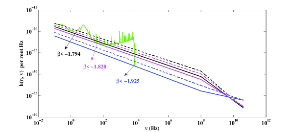
Figure 1: The spectrum of RGWs in usual case (solid lines) and thermal case (dashed lines) compared to the Hanford sensitivity (green line).

$$h(k,\eta_{0})=A\Big{(}\frac{k}{k_{H}}\Big{)}^{1+\beta-\beta_{s}}\Big{(}\frac{k_{s}}{k_{H}}\Big{)}^{\beta_{s}}\Big{(}\frac{k_{H}}{k_{2}}\Big{)}(1+z_{E})^{\frac{-2-\gamma}{\gamma}}\coth^{1/2}[\frac{k}{2T_{*}}],$$

$$\;\;\;k_{s}\leq k\leq k_{1}.$$ (11)

where $T=0.001\;Mpc^{-1}$6 , $T_{*}=1.19\times 10^{25}\;Mpc^{-1}$ 7 , $\gamma$ is $\Omega_{\Lambda}$ dependent parameter, and $\Omega_{\Lambda}$ is the energy density contrast. We take the value of redshift $z_{E}\sim 1.3$ and $\gamma\simeq 1.05$ 13 for $\Omega_{\Lambda}=0.692$ from Planck 2015 1 . By taking $k=2\pi\nu$, we can obtain $\nu_{E}=1.93\times 10^{-18}$ Hz, $\nu_{H}=2.28\times 10^{-18}$ Hz, $\nu_{2}=9.3\times 10^{-17}$ Hz, $\nu_{s}=10^{8}$ Hz and $\nu_{1}\simeq 4\times 10^{10}$ Hz 11 ; 14 .

One can get the constant $A$ without scalar running as follows 15

$$A=\frac{\Delta_{R}(k_{0})r^{1/2}}{(1+z_{E})^{\frac{-2-\gamma}{\gamma}}}(\frac{\nu_{H}}{\nu_{0}})^{\beta},$$ (12)

where $\Delta^{2}_{R}(k_{0})$ is the power spectrum of the curvature perturbation evaluated at the pivot wave number $k^{p}_{0}=k_{0}/a(\eta_{0})=0.002$ Mpc^-1 16 with corresponding physical frequency $\nu_{0}=3.09\times 10^{-18}$ Hz. The $\Delta^{2}_{R}(k_{0})=(2.464\pm 0.072\times 10^{-9})$ is given by WMAP9$+$eCMB$+$BAO$+$ $H_{0}$ 17 . The tensor to scalar ratio $r<0.11(95\%CL)$ is based on Planck measurement 18 . We take $r\simeq 0.1$ and also value of redshift $z_{E}=0.3$ for TT, TE, EE+lowP+lensing contribution in this work, see appendix.[A] for more details.

III The analysis of the spectrum

Let us now call the spectrum of the waves in the thermal case as ‘thermal spectrum’ . In this section we have supported and upgraded our previous result that obtained in 8 by comparision the thermal spectrum with the average measured sensitivity of Adv.LIGO (Hanford and Livingstone) and Dml. We are interested to the frequency range $\sim($10^-1Hz -10¹¹Hz). Therefore we plotted the spectrum by using eqs.(9-11) in figs.[1, 2]. Note that the amplitude rescaled to $h(\nu)/\sqrt{\nu}$ for comparison with Adv.LIGO. The fig.[1] and fig.[2] show the spectrum compared to the Hanford (green color) and Livingstone (red color) sensitivity respectively. The solid and dashed lines are stand for the usual and thermal spectrum respectively. We obtained upper bound on the $\beta$ at three points as a sample in both figures compared to Hanford and Livingstone sensitivity. The obtained diagrams tell us, there are some chances for detection of the thermal spectrum with modified amplitude in addition to the usual spectrum, see the intersection between the dashed lines and Hanford and Livingstone sensitivity in both figures. Also the obtained upper bounds on $\beta$ give us more information about the nature of the evolution of inflation stage.

On the other hand there is a procedure for detection based on Dml at GHz band 5 . The author in 5 is obtained the sensitivity of the Dml at the frequency $4.5$ GHz like:

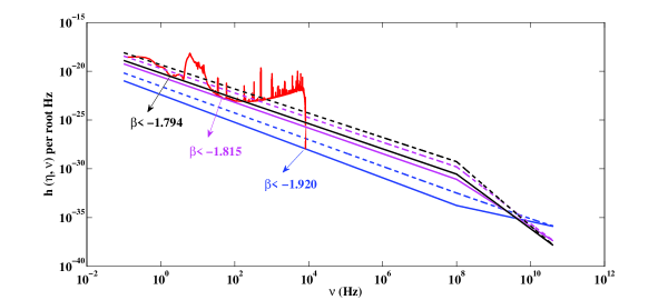
Figure 2: The spectrum of RGWs in usual case (solid lines) and thermal case (dashed lines) compared to the Livingstone sensitivity (red line).

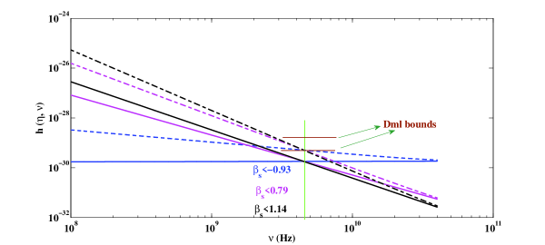
Figure 3: The high frequency range of fig.[2] compared to Dml sensitivity at $4.5$ GHz (green vertical line).

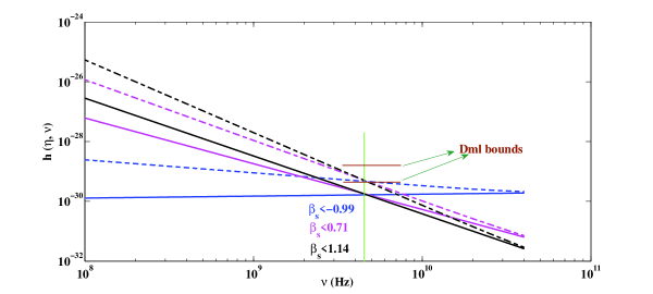
Figure 4: The high frequency range of fig.[1] compared to Dml sensitivity at $4.5$ GHz (green vertical line).

$$\sim(5.1\times 10^{-30}-1.6\times 10^{-29}).$$ (13)

He is believed that the Dml can not detect the RGWs due to the gap of $4\sim 5$ orders between the sensitivity of the Dml and the amplitude of the waves. Therefore he is recommended to upgrade the Dml by using some points that mentioned in 5 . In addition to those points, we claim that the problem of detection can remove by considering thermal spectrum. Using eq.(11), we plotted thermal spectrum (dashed lines) compared to the usual spectrum (solid lines) in the frequency range $\sim($10⁸Hz -10¹¹Hz) in figs.[4, 3]. The green vertical line stands for the frequency at $4.5$ GHz in both figures. The upper bounds on $\beta_{s}$ in fig.[4] (fig.[3]) obtained corresponding to the upper bounds on $\beta$ in fig.[1] (fig.[2]). For given $\beta,\beta_{s}$ the obtained usual and thermal amplitude in both figures are $\sim 1.7\times 10^{-30}$ and $\sim 5.1\times 10^{-30}$ at the frequency $4.5$ GHz respectively. Note that for given $\beta$ and lower $\beta_{s}$ according to the range of $\beta_{s}$ in figs.[4,3], the thermal amplitude will be further. Therefore based on the range in eq.(13) and obtaind usual amplitude $\sim 1.7\times 10^{-30}$, Dml can not detect the waves in the usual case as the author said in 5 . But by considering the thermal amplitude $\sim 5.1\times 10^{-30}$, the obtained diagrams tell us that we are lucky to detect the waves at the frequency $4.5$ GHz. Also the obtained upper bounds on $\beta_{s}$ give us more information about the nature of the evolution of the reheating stage.

IV Discussion and conclusion

The RGWs are generated before and during inflation stage. They contain valuable information about the early universe in the frequency range $\sim($10^-19Hz -10¹¹Hz). The thermal spectrum of RGWs causes the new amplitude that called ‘modified amplitude’. The obtained diagrams of the spectrum tell us, there are some chances for detection of the thermal spectrum in addition to the usual spectrum by using Adv.LIGO data of GW150914 and Dml. Also the $\beta$ and $\beta_{s}$ have an unique effect on the shape of the spectrum. We found some upper bounds on the $\beta$ and $\beta_{s}$ by comparison the usual and thermal spectrum with Adv.LIGO data of GW150914 and Dml. As this result about the upper bounds modified our information about the nature of the evolution of inflation and reheating stages.

Appendix A

The general solution of eq.(5) is a linear combination of the Hankel function with a generic power law for the scale factor $S=\eta^{u}$ given by

$$f_{k}(\eta)=A_{k}\sqrt{k\eta}H^{(1)}_{u-\frac{1}{2}}(k\eta)+B_{k}\sqrt{k\eta}H^{(2)}_{u-\frac{1}{2}}(k\eta).$$ (14)

We can write an exact solution $f_{k}(\eta)$ by matching its value and derivative at the joining points, for of a sequence of successive scale factors with different $u$ for a given model of the expansion of universe. The approximate solution of the spectrum of RGWs is usually computed in two limiting cases based on the waves are outside ($k^{2}\gg S^{\prime\prime}/S$, short wave approximation) or inside ($k^{2}\ll S^{\prime\prime}/S$, long wave approximation) of the barrier. For the RGWs outside the barrier the corresponding amplitude decrease as $h_{k}\propto 1/S(\eta)$ while for the waves inside the barrier, $h_{k}=C_{k}$ simply a constant. Therefore these results can be used to obtain the spectrum for the present stage of universe 11 ; s . The history of expansion of the universe can written as follows:

a) Inflation stage:

$$S(\eta)=l_{0}|\eta|^{1+\beta},\;\;\;\;\;\;-\infty<\eta\leq\eta_{1},$$ (15)

where $1+\beta<0$, $\eta<0$ and $l_{0}$ is a constant.

b) Reheating stage:

$$S(\eta)=S_{z}(\eta-\eta_{p})^{1+\beta_{s}},\;\;\;\;\;\;\eta_{1}<\eta\leq\eta_{s},$$ (16)

where $1+\beta_{s}>0$, see for more details 11 .

c) Radiation-dominated stage:

$$S(\eta)=S_{e}(\eta-\eta_{e}),\;\;\;\;\;\;\eta_{s}\leq\eta\leq\eta_{2}.$$ (17)

d) Matter-dominated stage:

$$S(\eta)=S_{m}(\eta-\eta_{m})^{2},\;\;\;\;\;\;\eta_{2}\leq\eta\leq\eta_{E},$$ (18)

where $\eta_{E}$ is the time when the dark energy density $\rho_{\Lambda}$ is equal to the matter energy density $\rho_{m}$. The value of redshift $z_{E}$ at $\eta_{E}$ is $(1+z_{E})=S(\eta_{0})/S(\eta_{E})\sim 1.3$ for TT, TE, EE+lowP+lensing contribution based on Planck 2015 1 where $\eta_{0}$ is the present time.

e) Accelerating stage:

$$S(\eta)=\ell_{0}|\eta-\eta_{a}|^{-\gamma},\;\;\;\;\;\;\eta_{E}\leq\eta\leq\eta_{0},$$ (19)

For normalization purpose of $S$, we put $|\eta_{0}-\eta_{a}|=1$ which fixes the $\eta_{a}$, and the constant $\ell_{0}$ is fixed by the following relation,

$$\frac{\gamma}{H_{0}}\equiv\Big{(}\frac{S^{2}}{S^{\prime}}\Big{)}_{\eta_{0}}=\ell_{0},$$ (20)

where $\ell_{0}$ is the Hubble radius at present with $H_{0}=67.8$ km s^-1Mpc^-1 from Planck 2015 1 . The wave number $k_{H}$ corresponding to the present Hubble radius is $k_{H}=2\pi S(\eta_{0})/\ell_{0}=2\pi\gamma$. There is another wave number $k_{E}=\frac{2\pi S(\eta_{E})}{1/H_{0}}=\frac{k_{H}}{1+z_{E}},$ that its wavelength at the time $\eta_{E}$ is the Hubble radius $1/H_{0}$. By matching $S$ and $S^{\prime}/S$ at the joint points, one gets

$$l_{0}=\ell_{0}b\zeta_{E}^{-(2+\beta)}\zeta_{2}^{\frac{\beta-1}{2}}\zeta_{s}^{\beta}\zeta_{1}^{\frac{\beta-\beta_{s}}{1+\beta_{s}}},$$ (21)

where $b\equiv|1+\beta|^{-(2+\beta)}$, $\zeta_{E}\equiv\frac{S(\eta_{0})}{S(\eta_{E})}$, $\zeta_{2}\equiv\frac{S(\eta_{E})}{S(\eta_{2})}$, $\zeta_{s}\equiv\frac{S(\eta_{2})}{S(\eta_{s})}$, and $\zeta_{1}\equiv\frac{S(\eta_{s})}{S(\eta_{1})}$. With these specifications, the functions $S(\eta)$ and $S^{\prime}(\eta)/S(\eta)$ are fully determined 11 ; 15 .

The power spectrum of RGWs is defined as

$$\int_{0}^{\infty}h^{2}(k,\eta)\frac{dk}{k}=\langle 0|h^{ij}({\bf x},\eta)h_{ij}({\bf x},\eta)|0\rangle.$$ (22)

Substituting eq.(II) in eq.(22) with same contribution of each polarization, we get

$$h(k,\eta)=\frac{4l_{pl}}{\sqrt{\pi}}k|h(\eta)|.$$ (23)

The spectrum at the present time $h(k,\eta_{0})$ can be obtained, provided the initial spectrum is specified. The initial amplitude of the spectrum is given by

$$h(k,\eta_{i})=A{\left(\frac{k}{k_{H}}\right)}^{2+\beta},$$ (24)

where the constant $A$ can be determined by quantum normalization 11 ; 15 .

Therefore the amplitude of the spectrum for different ranges of wave numbers are given by 11 ; 12 ; 15

$$h(k,\eta_{0})=A\Big{(}\frac{k}{k_{H}}\Big{)}^{2+\beta},\;\;\;k\leq k_{E},$$ (25)

$$h(k,\eta_{0})=A\Big{(}\frac{k}{k_{H}}\Big{)}^{\beta-\gamma}(1+z_{E})^{\frac{-2-\gamma}{\gamma}},\;\;\;k_{E}\leq k\leq k_{H},$$ (26)

$$h(k,\eta_{0})=A\Big{(}\frac{k}{k_{H}}\Big{)}^{\beta}(1+z_{E})^{\frac{-2-\gamma}{\gamma}},\;\;\;k_{H}\leq k\leq k_{2},$$ (27)

$$h(k,\eta_{0})=A\Big{(}\frac{k}{k_{H}}\Big{)}^{1+\beta}\Big{(}\frac{k_{H}}{k_{2}}\Big{)}(1+z_{E})^{\frac{-2-\gamma}{\gamma}},\;\;\;k_{2}\leq k\leq k_{s},$$ (28)

$$h(k,\eta_{0})=A\Big{(}\frac{k}{k_{H}}\Big{)}^{1+\beta-\beta_{s}}\Big{(}\frac{k_{s}}{k_{H}}\Big{)}^{\beta_{s}}\Big{(}\frac{k_{H}}{k_{2}}\Big{)}(1+z_{E})^{\frac{-2-\gamma}{\gamma}},$$

$$\;\;\;k_{s}\leq k\leq k_{1}.$$ (29)

Appendix B

An effective approach to deals with the thermal vacuum state is the thermo-field dynamics (TFD)34 . In this approach a tilde space is needed besides the usual Hilbert space, and the direct product space is made up of the these two spaces. Every operator and state in the Hilbert space has the corresponding counter part in the tilde space 34 . Therefore a thermal vacuum state can be defined as

$$|Tv\rangle={\cal T}(\theta_{k})|0\;\tilde{0}\rangle,$$ (30)

where

$${\cal T}(\theta_{k})=\mathrm{exp}[-\theta_{k}(a_{\bf{k}}\tilde{a}_{\bf{k}}-a_{\bf{k}}^{\dagger}\tilde{a}_{\bf{k}}^{\dagger})],$$ (31)

is the thermal operator and $|0\;\tilde{0}\rangle$ is the two mode vacuum state at zero temperature. The quantity $\theta_{k}$ is related to the average number of the thermal particle, $\bar{n}_{k}=\mathrm{sinh}^{2}\theta_{k}$. The $\bar{n}_{k}$ for given temperature T is provided by the Bose-Einstein distribution $\bar{n}_{k}=[\mathrm{exp}(k/T)-1]^{-1}$, where $\omega_{k}$ is the resonance frequency of the field, see Ref.8 for more details.

References

References

- (1) Ade P A R, Aghanim N et al, Planck Collaboration , [ arXiv:1502.01589v2] (2015).
- (2) https://www.elisascience.org/
- (3) http://losc.ligo.org/events/GW150914/.
- (4) http://www.et-gw.eu
- (5) Tong M l 2008 Phys.Rev.D 78 024041
- (6) Zhao W et al, 2009 Phys. Lett.B 680 411; Bhattacharya K et al, 2004 Phys. Rev. Lett. 97 251301
- (7) K. Wang, L. Santos, J. Q. Xia and W. Zhao, “Thermal gravitational-wave background in the general pre-inflationary scenario,” [arXiv:1608.04189 [astro-ph.CO]].
- (8) Siegel E R and Fry J N 2005 Phys. Lett.B 612 122.
- (9) Brax P and Bruck C 2003 Classical Quantum Gravity 20 R201, Kaluza T et al, 1921 Math. Phys. 1921 966 ; Arkani N-Hamed 1998 Phys. Lett.B 429 263 ; N. Arkani-Hamed et al, 1999 Phys. Rev. D 59 086004 ; Randall L and Sundrum R 1999 Phys. Rev. Lett. 83 3370 ; Randall L and Sundrum R 1999 Phys. Rev. Lett. 83 4690.
- (10) M. Gasperini, M. Giovannini and G. Veneziano, “Squeezed thermal vacuum and the maximum scale for inflation,” Phys. Rev. D 48, R439 (1993). [gr-qc/9306015].
- (11) Ghayour B and Suresh P K 2012 Class. Quantum Grav. 29 175009
- (12) Abbott B P, et al, 2016 Phys. Rev. Lett. 116 061102
- (13) Grishchuk L P 2001 Lect.Notes Phys. 562 167-194
- (14) Zhang Y et al, 2005 Class. Quantum Grav. 22 1383 -1394
- (15) Zhang Y et al, 2010 Phys. Rev.D 81 101501
- (16) Tong M 2013 Class. Quantum Grav. 30 055013
- (17) Tong M 2012 Class. Quantum Grav. 29 155006
- (18) Komatsu E et al, 2011 Astrophys. J. Suppl. 192 18
- (19) Bennett C L et al, Nine-Year Wilkinson Microwave Anisotropy Probe (WMAP) Observations: Final Maps and Results, [arXiv:1212.5225 [astro-ph.CO]].
- (20) Planck Collaboration, Planck 2013 results. XXII. Constraints on infation ; 2014 Astron. Astrophys. 571 A22 [arXiv:1303.5082v3].
- (21) Zhang Y et al, 2006 Class. Quantum Grav. 23 3783-3800
- (22) Umezawa H and Yamanaka Y 1988 Adv. Phys.37 531; Fearm H and Collett M J 1988 J. Mod. Opt.35 553; Chaturvedi S et al 1990 Phys. Rev.A 41 3969; J-Vogt Oz et al 1991 J. Mod. Opt. 38 2339