Robustness of classifiers: from adversarial to random noise
Abstract
Several recent works have shown that state-of-the-art classifiers are vulnerable to worst-case (i.e., adversarial) perturbations of the datapoints. On the other hand, it has been empirically observed that these same classifiers are relatively robust to random noise. In this paper, we propose to study a semi-random noise regime that generalizes both the random and worst-case noise regimes. We propose the first quantitative analysis of the robustness of nonlinear classifiers in this general noise regime. We establish precise theoretical bounds on the robustness of classifiers in this general regime, which depend on the curvature of the classifier’s decision boundary. Our bounds confirm and quantify the empirical observations that classifiers satisfying curvature constraints are robust to random noise. Moreover, we quantify the robustness of classifiers in terms of the subspace dimension in the semi-random noise regime, and show that our bounds remarkably interpolate between the worst-case and random noise regimes. We perform experiments and show that the derived bounds provide very accurate estimates when applied to various state-of-the-art deep neural networks and datasets. This result suggests bounds on the curvature of the classifiers’ decision boundaries that we support experimentally, and more generally offers important insights onto the geometry of high dimensional classification problems.
1 Introduction
State-of-the-art classifiers, especially deep networks, have shown impressive classification performance on many challenging benchmarks in visual tasks [10] and speech processing [8]. An equally important property of a classifier that is often overlooked is its robustness in noisy regimes, when data samples are perturbed by noise. The robustness of a classifier is especially fundamental when it is deployed in real-world, uncontrolled, and possibly hostile environments. In these cases, it is crucial that classifiers exhibit good robustness properties. In other words, a sufficiently small perturbation of a datapoint should ideally not result in altering the estimated label of a classifier. State-of-the-art deep neural networks have recently been shown to be very unstable to worst-case perturbations of the data (or equivalently, adversarial perturbations) [18]. In particular, despite the excellent classification performances of these classifiers, well-sought perturbations of the data can easily cause misclassification, since data points often lie very close to the decision boundary of the classifier. Despite the importance of this result, the worst-case noise regime that is studied in [18] only represents a very specific type of noise. It furthermore requires the full knowledge of the classification model, which may be a hard assumption in practice.
In this paper, we precisely quantify the robustness of nonlinear classifiers in two practical noise regimes, namely random and semi-random noise regimes. In the random noise regime, datapoints are perturbed by noise with random direction in the input space. The semi-random regime generalizes this model to random subspaces of arbitrary dimension, where a worst-case perturbation is sought within the subspace. In both cases, we derive bounds that precisely describe the robustness of classifiers in function of the curvature of the decision boundary. We summarize our contributions as follows:
-
•
In the random regime, we show that the robustness of classifiers behaves as times the distance from the datapoint to the classification boundary (where denotes the dimension of the data) provided the curvature of the decision boundary is sufficiently small. This result highlights the blessing of dimensionality for classification tasks, as it implies that robustness to random noise in high dimensional classification problems can be achieved, even at datapoints that are very close to the decision boundary.
-
•
This quantification notably extends to the general semi-random regime, where we show that the robustness precisely behaves as times the distance to boundary, with the dimension of the subspace. This result shows in particular that, even when is chosen as a small fraction of the dimension , it is still possible to find small perturbations that cause data misclassification.
-
•
We empirically show that our theoretical estimates are very accurately satisfied by state-of-the-art deep neural networks on various sets of data. This in turn suggests quantitative insights on the curvature of the decision boundary that we support experimentally through the visualization and estimation on two-dimensional sections of the boundary.
The robustness of classifiers to noise has been the subject of intense research. The robustness properties of SVM classifiers have been studied in [20] for example, and robust optimization approaches for constructing robust classifiers have been proposed to minimize the worst possible empirical error under noise disturbance [1, 11]. More recently, following the recent results on the instability of deep neural networks to worst-case perturbations [18], several works have provided explanations of the phenomenon [4, 6, 15, 19], and designed more robust networks [7, 9, 21, 14, 16, 13]. In [19], the authors provide an interesting empirical analysis of the adversarial instability, and show that adversarial examples are not isolated points, but rather occupy dense regions of the pixel space. In [5], state-of-the-art classifiers are shown to be vulnerable to geometrically constrained adversarial examples. Our work differs from these works, as we provide a theoretical study of the robustness of classifiers to random and semi-random noise in terms of the robustness to adversarial noise. In [4], a formal relation between the robustness to random noise, and the worst-case robustness is established in the case of linear classifiers. Our result therefore generalizes [4] in many aspects, as we study general nonlinear classifiers, and robustness to semi-random noise. Finally, it should be noted that the authors in [6] conjecture that the “high linearity” of classification models explains their instability to adversarial perturbations. The objective and approach we follow here is however different, as we study theoretical relations between the robustness to random, semi-random and adversarial noise.
2 Definitions and notations
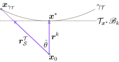
Let be an -class classifier. Given a datapoint , the estimated label is obtained by , where is the component of that corresponds to the class. Let be an arbitrary subspace of of dimension . Here, we are interested in quantifying the robustness of with respect to different noise regimes. To do so, we define to be the perturbation in of minimal norm that is required to change the estimated label of at .111Perturbation vectors sending a datapoint exactly to the boundary are assumed to change the estimated label of the classifier.
| (1) |
Note that can be equivalently written
| (2) |
When is the adversarial (or worst-case) perturbation defined in [18], which corresponds to the (unconstrained) perturbation of minimal norm that changes the label of the datapoint . In other words, corresponds to the minimal distance from to the classifier boundary. In the case where , only perturbations along are allowed. The robustness of at along is naturally measured by the norm . Different choices for permit to study the robustness of in two different regimes:
-
•
Random noise regime: This corresponds to the case where is a one-dimensional subspace () with direction , where is a random vector sampled uniformly from the unit sphere . Writing it explicitly, we study in this regime the robustness quantity defined by , where is a vector sampled uniformly at random from the unit sphere .
-
•
Semi-random noise regime: In this case, the subspace is chosen randomly, but can be of arbitrary dimension .222A random subspace is defined as the span of independent vectors drawn uniformly at random from . We use the semi-random terminology as the subspace is chosen randomly, and the smallest vector that causes misclassification is then sought in the subspace. It should be noted that the random noise regime is a special case of the semi-random regime with a subspace of dimension . We differentiate nevertheless between these two regimes for clarity.
In the remainder of the paper, the goal is to establish relations between the robustness in the random and semi-random regimes on the one hand, and the robustness to adversarial perturbations on the other hand. We recall that the latter quantity captures the distance from to the classifier boundary, and is therefore a key quantity in the analysis of robustness.
In the following analysis, we fix to be a datapoint classified as . To simplify the notation, we remove the explicit dependence on in our notations (e.g., we use instead of and instead of ), and it should be implicitly understood that all our quantities pertain to the fixed datapoint .
3 Robustness of affine classifiers
We first assume that is an affine classifier, i.e., for a given and .
The following result shows a precise relation between the robustness to semi-random noise, and the robustness to adversarial perturbations, .
Theorem 1.
Let and be a random -dimensional subspace of , and be a -class affine classifier. Let
| (3) | ||||
| (4) |
The following inequalities hold between the robustness to semi-random noise , and the robustness to adversarial perturbations :
| (5) |
with probability exceeding .
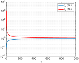
The proof can be found in the appendix. Our upper and lower bounds depend on the functions and that control the inequality constants (for , fixed). It should be noted that and are independent of the data dimension . Fig. 1 shows the plots of and as functions of , for a fixed . It should be noted that for sufficiently large , and are very close to (e.g., and belong to the interval for in the settings of Fig. 1). The interval is however (unavoidably) larger when .
The result in Theorem 1 shows that in the random and semi-random noise regimes, the robustness to noise is precisely related to by a factor of . Specifically, in the random noise regime (), the magnitude of the noise required to misclassify the datapoint behaves as with high probability, with constants in the interval . Our results therefore show that, in high dimensional classification settings, affine classifiers can be robust to random noise, even if the datapoint lies very closely to the decision boundary (i.e., is small). In the semi-random noise regime with sufficiently large (e.g., ), we have with high probability, as the constants for sufficiently large . Our bounds therefore “interpolate” between the random noise regime, which behaves as , and the worst-case noise . More importantly, the square root dependence is also notable here, as it shows that the semi-random robustness can remain small even in regimes where is chosen to be a very small fraction of . For example, choosing a small subspace of dimension results in semi-random robustness of with high probability, which might still not be perceptible in complex visual tasks. Hence, for semi-random noise that is mostly random and only mildly adversarial (i.e., the subspace dimension is small), affine classifiers remain vulnerable to such noise.
4 Robustness of general classifiers
4.1 Decision boundary curvature
We now consider the general case where is a nonlinear classifier. We derive relations between the random and semi-random robustness and worst-case robustness using properties of the classifier’s boundary. Let and be two arbitrary classes; we define the pairwise boundary as the boundary of the binary classifier where only classes and are considered. Formally, the decision boundary reads as follows:
The boundary separates between two regions of , namely and , where the estimated label of the binary classifier is respectively and . Specifically, we have
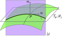
We assume for the purpose of this analysis that the boundary is smooth. We are now interested in the geometric properties of the boundary, namely its curvature. There are many notions of curvature that one can define on hypersurfaces [12]. In the simple case of a curve in a two-dimensional space, the curvature is defined as the inverse of the radius of the so-called oscullating circle. One way to define curvature for high-dimensional hypersurfaces is by taking normal sections of the hypersurface, and looking at the curvature of the resulting planar curve (see Fig. 4). We however introduce a notion of curvature that is specifically suited to the analysis of the decision boundary of a classifier. Informally, our curvature captures the global bending of the decision boundary by inscribing balls in the regions separated by the decision boundary.
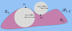
We now formally define this notion of curvature. For a given , we define to be the radius of the largest open ball included in the region that intersects with at ; i.e.,
| (6) |
where is the open ball in of center and radius . An illustration of this quantity in two dimensions is provided in Fig. 2. It is not hard to see that any ball centered in and included in will have its tangent space at coincide with the tangent of the decision boundary at the same point.
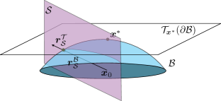
It should further be noted that the definition in Eq. (6) is not symmetric in and ; i.e., as the radius of the largest ball one can inscribe in both regions need not be equal. We therefore define the following symmetric quantity , where the worst-case ball inscribed in any of the two regions is considered:
This definition describes the curvature of the decision boundary locally at by fitting the largest ball included in one of the regions. To measure the global curvature, the worst-case radius is taken over all points on the decision boundary, i.e.,
| (7) | ||||
| (8) |
The curvature is simply defined as the inverse of the worst-case radius over all points on the decision boundary.
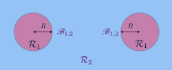
In the case of affine classifiers, we have , as it is possible to inscribe balls of infinite radius inside each region of the space. When the classification boundary is a union of (sufficiently distant) spheres with equal radius (see Fig. 3), the curvature . In general, the quantity provides an intuitive way of describing the nonlinearity of the decision boundary by fitting balls inside the classification regions.
In the following section, we show a precise characterization of the robustness to semi-random and random noise of nonlinear classifiers in terms of the curvature of the decision boundaries .
4.2 Robustness to random and semi-random noise
We now establish bounds on the robustness to random and semi-random noise in the binary classification case. Let be a datapoint classified as . We first study the binary classification problem, where only classes and are considered. To simplify the notation, we let be the decision boundary between classes and . In the case of the binary classification problem where classes and are considered, the semi-random robustness and adversarial (or worst-case) robustness defined in Eq. (2) can be re-written as follows:
| (9) | ||||
For a randomly chosen subspace, is the random or semi-random robustness of the classifier, in the setting where only the two classes and are considered. Likewise, denotes the worst-case robustness in this setting. It should be noted that the global quantities and are obtained from and by taking the vectors with minimum norm over all classes .
The following result gives upper and lower bounds on the ratio in function of the curvature of the boundary separating class and .
Theorem 2.
The proof can be found in the appendix. This result shows that the bounds relating the robustness to random and semi-random noise to the worst-case robustness can be extended to nonlinear classifiers, provided the curvature of the boundary is sufficiently small. In the case of linear classifiers, we have , and we recover the result for affine classifiers from Theorem 1.
To extend this result to multi-class classification, special care has to be taken. In particular, if denotes a class that has no boundary with class , we have , and the previous curvature condition cannot be satisfied. It is therefore crucial to exclude such classes that have no boundary in common with class , or more generally, boundaries that are far from class . We define the set of excluded classes where is large
| (11) |
Note that is independent of , and depends only on , and . Moreover, the constants in (11) were chosen for simplicity of exposition.
Assuming a curvature constraint only on the close enough classes, the following result establishes a simplified relation between and .
Corollary 1.
Let be a random -dimensional subspace of . Assume that, for all , we have
| (12) |
Then, we have
| (13) |
with probability larger than .
Under the curvature condition in (12) on the boundaries between and classes in , our result shows that the robustness to random and semi-random noise exhibits the same behavior that has been observed earlier for linear classifiers in Theorem 1. In particular, is precisely related to the adversarial robustness by a factor of . In the random regime (), this factor becomes , and shows that in high dimensional classification problems, classifiers with sufficiently flat boundaries are much more robust to random noise than to adversarial noise. More precisely, the addition of a sufficiently small random noise does not change the label of the image, even if the image lies very closely to the decision boundary (i.e., is small). However, in the semi-random regime where an adversarial perturbation is found on a randomly chosen subspace of dimension , the factor that relates to shows that robustness to semi-random noise might not be achieved even if is chosen to be a tiny fraction of (e.g., ). In other words, if a classifier is highly vulnerable to adversarial perturbations, then it is also vulnerable to noise that is overwhelmingly random and only mildly adversarial (i.e. worst-case noise sought in a random subspace of low dimensionality ).
It is important to note that the curvature condition in (12) is not an assumption on the curvature of the global decision boundary, but rather an assumption on the decision boundaries between pairs of classes. The distinction here is significant, as junction points where two decision boundaries meet might actually have a very large (or infinite) curvature (even in linear classification settings), and the curvature condition in (12) typically does not hold for this global curvature definition. We refer to our experimental section for a visualization of this phenomenon.
We finally stress that our results in Theorem 2 and Corollary 1 are applicable to any classifier, provided the decision boundaries are smooth. If we assume prior knowledge on the considered family of classifiers and their decision boundaries (e.g., the decision boundary is a union of spheres in ), similar bounds can further be derived under less restrictive curvature conditions (compared to Eq. (12)).
5 Experiments
5.1 Experimental results
We now evaluate the robustness of different image classifiers to random and semi-random perturbations, and assess the accuracy of our bounds on various datasets and state-of-the-art classifiers. Specifically, our theoretical results show that the robustness of classifiers satisfying the curvature property precisely behaves as . We first check the accuracy of these results in different classification settings. For a given classifier and subspace dimension , we define
where is chosen randomly for each sample and denotes the test set. This quantity provides indication to the accuracy of our estimate of the robustness, and should ideally be equal to (for sufficiently large ). Since is a random quantity (because of ), we report both its mean and standard deviation for different networks in Table 1. It should be noted that finding and involves solving the optimization problem in (1). We have used a similar approach to [14] to find subspace minimal perturbations. For each network, we estimate the expectation by averaging on 1000 random samples, with also chosen randomly for each sample.
| Classifier | 1 | |||||
|---|---|---|---|---|---|---|
| LeNet (MNIST) | ||||||
| LeNet (CIFAR-10) | ||||||
| VGG-F (ImageNet) | ||||||
| VGG-19 (ImageNet) | ||||||
Observe that is suprisingly close to 1, even when is a small fraction of . This shows that our quantitative analysis provide very accurate estimates of the robustness to semi-random noise. We visualize the robustness to random noise, semi-random noise (with ) and worst-case perturbations on a sample image in Fig. 5. While random noise is clearly perceptible due to the factor, semi-random noise becomes much less perceptible even with a relatively small value of , thanks to the factor that attenuates the required noise to misclassify the datapoint. It should be noted that the robustness of neural networks to adversarial perturbations has previously been observed empirically in [18], but we provide here a quantitative and generic explanation for this phenomenon.
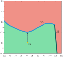
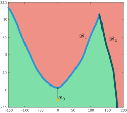
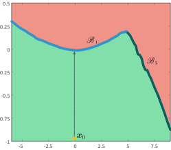
The high accuracy of our bounds for different state-of-the-art classifiers, and different datasets suggest that the decision boundaries of these classifiers have limited curvature , as this is a key assumption of our theoretical findings. To support the validity of this curvature hypothesis in practice, we visualize two-dimensional sections of the classifiers’ boundary in Fig. 6 in three different settings. Note that we have opted here for a visualization strategy rather than the numerical estimation of , as the latter quantity is difficult to approximate in practice in high dimensional problems. In Fig. 6, is chosen randomly from the test set for each data set, and the decision boundaries are shown in the plane spanned by and , where is a random direction (i.e., ). Different colors on the boundary correspond to boundaries with different classes. It can be observed that the curvature of the boundary is very small except at “junction” points where the boundary of two different classes intersect. Our curvature assumption in Eq. (12), which only assumes a bound on the curvature of the decision boundary between pairs of classes and (but not on the global decision boundary that contains junctions with high curvature) is therefore adequate to the decision boundaries of state-of-the-art classifiers according to Fig. 6. Interestingly, the assumption in Corollary 1 is satisfied by taking to be an empirical estimate of the curvature of the planar curves in Fig. 6 (a) for the dimension of the subspace being a very small fraction of ; e.g., . While not reflecting the curvature that drives the assumption of our theoretical analysis, this result still seems to suggest that the curvature assumption holds in practice, and that the curvature of such classifiers is therefore very small. It should be noted that a related empirical observation was made in [6]; our work however provides a precise quantitative analysis on the relation between the curvature and the robustness in the semi-random noise regime.
We now show a simple demonstration of the vulnerability of classifiers to semi-random noise in Fig. 7, where a structured message is hidden in the image and causes data misclassification. Specifically, we consider to be the span of random translated and scaled versions of words “NIPS”, “SPAIN” and “2016” in an image, such that . The resulting perturbations in the subspace are therefore linear combinations of these words with different intensities.333This example departs somehow from the theoretical framework of this paper, where random subspaces were considered. However, this empirical example suggests that the theoretical findings in this paper seem to approximately hold when the subspace have statistics that are close to a random subspace. The perturbed image shown in Fig. 7 (c) is clearly indistinguishable from Fig. 7 (a). This shows that imperceptibly small structured messages can be added to an image causing data misclassification.
6 Conclusion
In this work, we precisely characterized the robustness of classifiers in a novel semi-random noise regime that generalizes the random noise regime. Specifically, our bounds relate the robustness in this regime to the robustness to adversarial perturbations. Our bounds depend on the curvature of the decision boundary, the data dimension, and the dimension of the subspace to which the perturbation belongs. Our results show, in particular, that when the decision boundary has a small curvature, classifiers are robust to random noise in high dimensional classification problems (even if the robustness to adversarial perturbations is relatively small). Moreover, for semi-random noise that is mostly random and only mildly adversarial (i.e., the subspace dimension is small), our results show that state-of-the-art classifiers remain vulnerable to such perturbations. To improve the robustness to semi-random noise, our analysis encourages to impose geometric constraints on the curvature of the decision boundary, as we have shown the existence of an intimate relation between the robustness of classifiers and the curvature of the decision boundary.
Acknowledgments
We would like to thank the anonymous reviewers for their helpful comments. We thank Omar Fawzi and Louis Merlin for the fruitful discussions. We also gratefully acknowledge the support of NVIDIA Corporation with the donation of the Tesla K40 GPU used for this research. This work has been partly supported by the Hasler Foundation, Switzerland, in the framework of the CORA project.
References
- Caramanis et al., [2012] Caramanis, C., Mannor, S., and Xu, H. (2012). Robust optimization in machine learning. In Sra, S., Nowozin, S., and Wright, S. J., editors, Optimization for machine learning, chapter 14. Mit Press.
- Chatfield et al., [2014] Chatfield, K., Simonyan, K., Vedaldi, A., and Zisserman, A. (2014). Return of the devil in the details: Delving deep into convolutional nets. In British Machine Vision Conference.
- Dasgupta and Gupta, [2003] Dasgupta, S. and Gupta, A. (2003). An elementary proof of a theorem of johnson and lindenstrauss. Random Structures & Algorithms, 22(1):60–65.
- Fawzi et al., [2015] Fawzi, A., Fawzi, O., and Frossard, P. (2015). Analysis of classifiers’ robustness to adversarial perturbations. CoRR, abs/1502.02590.
- Fawzi and Frossard, [2015] Fawzi, A. and Frossard, P. (2015). Manitest: Are classifiers really invariant? In British Machine Vision Conference (BMVC), pages 106.1–106.13.
- Goodfellow et al., [2015] Goodfellow, I. J., Shlens, J., and Szegedy, C. (2015). Explaining and harnessing adversarial examples. In International Conference on Learning Representations (ICLR).
- Gu and Rigazio, [2014] Gu, S. and Rigazio, L. (2014). Towards deep neural network architectures robust to adversarial examples. arXiv preprint arXiv:1412.5068.
- Hinton et al., [2012] Hinton, G. E., Deng, L., Yu, D., Dahl, G. E., Mohamed, A., Jaitly, N., Senior, A., Vanhoucke, V., Nguyen, P., Sainath, T. N., and Kingsbury, B. (2012). Deep neural networks for acoustic modeling in speech recognition: The shared views of four research groups. IEEE Signal Process. Mag., 29(6):82–97.
- Huang et al., [2015] Huang, R., Xu, B., Schuurmans, D., and Szepesvári, C. (2015). Learning with a strong adversary. CoRR, abs/1511.03034.
- Krizhevsky et al., [2012] Krizhevsky, A., Sutskever, I., and Hinton, G. E. (2012). Imagenet classification with deep convolutional neural networks. In Advances in neural information processing systems (NIPS), pages 1097–1105.
- Lanckriet et al., [2003] Lanckriet, G., Ghaoui, L., Bhattacharyya, C., and Jordan, M. (2003). A robust minimax approach to classification. The Journal of Machine Learning Research, 3:555–582.
- Lee, [2009] Lee, J. M. (2009). Manifolds and differential geometry, volume 107. American Mathematical Society Providence.
- Luo et al., [2015] Luo, Y., Boix, X., Roig, G., Poggio, T., and Zhao, Q. (2015). Foveation-based mechanisms alleviate adversarial examples. arXiv preprint arXiv:1511.06292.
- Moosavi-Dezfooli et al., [2016] Moosavi-Dezfooli, S.-M., Fawzi, A., and Frossard, P. (2016). Deepfool: a simple and accurate method to fool deep neural networks. In IEEE Conference on Computer Vision and Pattern Recognition (CVPR).
- Sabour et al., [2016] Sabour, S., Cao, Y., Faghri, F., and Fleet, D. J. (2016). Adversarial manipulation of deep representations. In International Conference on Learning Representations (ICLR).
- Shaham et al., [2015] Shaham, U., Yamada, Y., and Negahban, S. (2015). Understanding adversarial training: Increasing local stability of neural nets through robust optimization. arXiv preprint arXiv:1511.05432.
- Simonyan and Zisserman, [2014] Simonyan, K. and Zisserman, A. (2014). Very deep convolutional networks for large-scale image recognition. In International Conference on Learning Representations (ICLR).
- Szegedy et al., [2014] Szegedy, C., Zaremba, W., Sutskever, I., Bruna, J., Erhan, D., Goodfellow, I., and Fergus, R. (2014). Intriguing properties of neural networks. In International Conference on Learning Representations (ICLR).
- Tabacof and Valle, [2016] Tabacof, P. and Valle, E. (2016). Exploring the space of adversarial images. IEEE International Joint Conference on Neural Networks.
- Xu et al., [2009] Xu, H., Caramanis, C., and Mannor, S. (2009). Robustness and regularization of support vector machines. The Journal of Machine Learning Research, 10:1485–1510.
- Zhao and Griffin, [2016] Zhao, Q. and Griffin, L. D. (2016). Suppressing the unusual: towards robust cnns using symmetric activation functions. arXiv preprint arXiv:1603.05145.
Appendix
A.1 Proof of Theorem 1 (affine classifiers)
Lemma 1 ([3]).
Let be a point chosen uniformly at random from the surface of the -dimensional sphere . Let the vector be the projection of onto its first coordinates, with . Then,
-
1.
If , then
(14) -
2.
If , then
(15)
Lemma 2.
Let be a random vector uniformly drawn from the unit sphere , and be the projection matrix onto the first coordinates. Then,
| (16) |
with , and .
Proof.
Note first that the upper bound of Lemma 1 can be bounded as follows:
| (17) |
using . We find such that , or equivalently, . It is easy to see that when , the inequality holds. Note however that does not converge to as . We therefore need to derive a tighter bound for this regime. Using the inequality for , it follows that the inequality holds for . In this case, we have , as . We take our lower bound to be the max of both derived bounds (the latter is more appropriate for large , whereas the former is tighter for small ).
For , note that the requirement is equivalent to . By setting , this condition is equivalent to , or equivalently, , with . The function is positive on . Hence, satisfies , which concludes the proof. ∎
We now prove our main theorem that we recall as follows:
Theorem 1.
Let be a random -dimensional subspace of . The following inequalities hold between the norms of semi-random perturbation and the worst-case perturbation . Let , and .
| (18) |
with probability exceeding .
Proof.
For the linear case, and can be computed in closed form. We recall that, for any subspace , we have
| (19) |
where was defined in Eq. (9). In particular, when , we have
| (20) |
Let . Define, for the sake of readability
Note that
| (21) |
The projection of a fixed vector in onto a random dimensional subspace is equivalent (up to a unitary transformation ) to the projection of a random vector uniformly sampled from into a fixed subspace. Let be the projection onto the first coordinates. We have
| (22) |
Hence, we have
| (23) |
where is a random vector distributed uniformly in the unit sphere . We apply Lemma 2, and obtain
| (24) |
Hence,
| (25) |
Using the multi-class extension in Lemma 3, we conclude that
| (26) |
∎
Lemma 3 (Binary case to multiclass).
Assume that, for all
| (27) |
Then, we have
| (28) |
Proof.
Let . Note that we have . Moreover, we use a union bound to bound the the other bad event probability:
| (29) |
We conclude by using the fact that
| (31) |
∎
A.2 Proof of Theorem 2 and Corollary 1 (nonlinear classifiers)
First, we present an important geometric lemma and then use it to bound . For the sake of the general readability of the section, some auxiliary results are given in Section A.3.
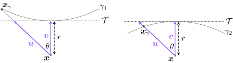
In the following result, we show that, when the curvature of a planar curve is constant and sufficiently small, the distance between a point and the curve at a specific direction is well approximated by the distance between and a straight line (see Fig. 8 for an illustration).
Lemma 4.
Let be a planar curve of constant curvature . We denote by the distance between a point and the curve . Denote moreover by the tangent to at the closest point to (see Fig. 8). Let be the angle between and as depicted in Fig. 8. We assume that . We have
| (32) |
Moreover, if
then, the following upper bound holds
| (33) |
We can set and .
Proof of upper bound.
We consider two distinct cases for the curve . In the case where is concave-shaped (Fig. 8, right figure), we have
and the upper bound in Eq. (33) directly holds. We therefore focus on the case where is convex-shaped as illustrated in the left figure of Fig. 8. Define , one can write using simple geometric inspection
| (34) |
where . The discriminant of the second order equation (with variable ) is equal to
We have as satisfies the two assumptions and . The smallest solution of this second order equation is given as follows
| (35) |
Using some simple algebraic manipulations, we obtain
| (36) |
Using the inequality in Lemma 73 together with the two assumptions, we get
| (37) |
With simple trigonometric identities, the above expression can be simplified to
| (38) |
We expand this quantity, and obtain
| (39) |
Since , we have
| (40) |
According to the assumptions , therefore
| (41) |
Since , one can finally conclude on the upper bound
| (42) |
∎
Proof of lower bound.
When the curve is convex shaped (Fig. 8 left), we have , and the desired lower bound holds. We focus therefore on the case where has a concave shape, and coincides with with (see Fig. 8 right). The following equation holds using simple geometric arguments
| (43) |
where . Solving this second order equation gives
| (44) |
After some algebraic manipulations, we get
| (45) |
Using the inequality in Lemma 74, together with the fact that , we obtain
| (46) |
Using simple trigonometric identities, the above expression is simplified to
| (47) |
When expanding it, we obtain
| (48) |
Since , we have
| (49) |
Using again the assumption , we obtain
| (50) |
Since , one can rewrite it as
| (51) |
which completes the proof. ∎
We now use the previous lemma to bound the semi-random robustness of the classifier, i.e. , to the worst-case robustness in the case where the curvature is sufficiently small.
Theorem 2.
Let be a random -dimensional subspace of . Define , and let . Assuming that , the following inequalities hold between and the worst-case perturbation
| (52) |
with probability larger than . The constants can be taken .

Proof of upper bound.
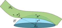
Denote by the point belonging to the boundary that is closest to the original data point . By definition of the curvature (see Eq. 7), there exists a point such that the ball centered at and of radius is inscribed in the region (see Fig. 9 (a)).444For a fixed point on the boundary, the maximal radius might not be achieved. To prove the result in the general case where the supremum is not achieved, one can consider instead a sequence converging to , such that the balls of radius and intersecting the boundary at are included in . The same proof and results follow by taking the limit on the bounds derived with ball of radius .
Observe that the worst-case perturbation along any subspace that reaches the ball is larger than the perturbation along that reaches the region , as . Therefore, any upper bound derived when the boundary is the sphere of radius ; i.e., is also a valid upper bound for boundary (see Fig. 9 (a)). It is therefore sufficient to derive an upper bound in the worst case scenario where the boundary , and we consider this case for the remainder of the proof of the upper bound.
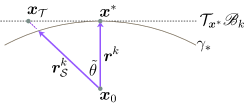
We now consider the linear classifier whose boundary is tangent to at . For the random subspace , we denote by the worst-case subspace perturbation for this linear classifier. We then focus on the intersection between the boundary and the two-dimensional plane spanned by the vectors and . This normal section of the boundary cuts the ball through its center as the tangent spaces of the decision boundary and the ball coincide. See Fig. 9 for a clarifying figure of this two-dimensional cross-section. We define the angle as denoted in Fig. 9, such that .
We apply our result on linear classifiers in Theorem 1 for the tangent classifier. We have
| (53) |
with probability exceeding . Hence, using and the assumption of the theorem, we deduce that
with probability exceeding . Note moreover that
Hence, the assumptions of Lemma 4 hold with probability larger than . Using the notations of Fig. 9, we therefore obtain from Lemma 4
| (54) |
with probability larger than .
Proof of the lower bound.
We now consider the ball of center and radius that is included in the region . Since the ball is, by definition, included in the region , the worst-case scenario for the lower bound on occurs whenever the decision boundary coincides with the ball (see Fig. 10 (a)). We consider this case in the remainder of the proof.
To derive the lower bound, we consider the cross-section spanned by the vectors and (Fig. 10 (b)). We have ; using the lower bound of Lemma 4, we obtain
| (56) |
for any . Observe moreover that
Hence, the following bound holds:
Let denote the worst-case perturbation belonging to subspace for the linear classifier . It is not hard to see that is collinear to (see Lemma 6 for a proof). Hence, we have . By applying our result on linear classifiers in Theorem 1 for the tangent classifier , we have:
We therefore conclude that
which concludes the proof of the lower bound.
∎
The goal is now to extend the previous result, derived for binary classifiers, to the multiclass classification case. To do so, we show the following lemma.
Lemma 5 (Binary case to multiclass).
Let . Define the deterministic set
| (57) |
Assume that, for all , we have
| (58) |
and that
| (59) |
Then, we have
| (60) |
Proof.
Note first that
| (61) |
We now focus on bounding the other bad event probability . We have
| (62) |
The first probability can be bounded as follows:
| (63) |
The second probability can also be bounded in the following way
| (64) |
Observe that, for , we have . Hence, we conclude that
| (65) | ||||
| (66) |
∎
Corollary 1.
Let be a random -dimensional subspace of . Assume that, for all , we have
| (67) |
Then, we have
| (68) |
with probability larger than .
A.3 Useful results
Lemma 6.
Let , and denote the closest point to on the sphere (see Fig. 11). Let be the tangent space to at . For an arbitrary subspace , let and denote the worst-case perturbations of on the subspace , when the decision boundaries are respectively and . Then, the two perturbations and are collinear.
Proof.
Assuming the center of the ball is the origin, the points on the sphere satisfy equation: , where denotes the radius. Hence, the perturbation is given by
| (72) |
By equating the gradient of Lagrangian of the above constrained optimization problem to zero, we obtain the following necessary optimality condition
It should further be noted that . Indeed, if had a component orthogonal to , the projection of onto would have strictly lower norm, while still satisfying the condition in Eq.(72). Hence, the necessary condition of optimality becomes
from which we conclude that is collinear to .
It should further be noted that can be computed in closed form, and is collinear to , which is itself collinear to , as the the center of the ball was assumed to be the origin. This concludes the proof. ∎
Lemma 7.
If ,
| (73) |
Lemma 8.
If ,
| (74) |