Hierarchical follow-up of sub-threshold candidates of an all-sky Einstein@Home search for continuous gravitational waves on LIGO sixth science run data

Abstract

We report results of an all-sky search for periodic gravitational waves with frequency between 50 and 510 Hz from isolated compact objects, e.g. neutron stars. A new hierarchical multi-stage approach is taken, supported by the computing power of the Einstein@Home  project, allowing to probe more deeply than ever before. 16 million sub-threshold candidates from the initial search S6BucketStage0 are followed up in three stages. None of those candidates is consistent with an isolated gravitational wave emitter, and 90% confidence level upper limits are placed on the amplitudes of continuous waves from the target population. Between 170.5 and 171  Hz we set the most constraining 90% confidence upper limit on the strain amplitude $h_{0}$ at 4.3 $\times 10^{-25}$, while at the high end of our frequency range we achieve an upper limit of 7.6 $\times 10^{-25}$. These are the most constraining all-sky upper limits to date and constrain the ellipticity of rotating compact objects emitting at $300$ Hz at a distance $D$ to less than 6 $\times 10^{-7}$$\left[D\over{100~{}\textrm{pc}}\right]$.

I Introduction

The beauty of continuous signals is that, even if a candidate is not significant enough to be recognised as a real signal after a first semi-coherent search, it is still possible to improve its significance to the level necessary to claim a detection after a series of follow-up searches. Hierarchical approaches were first proposed in the late 90s and developed over a number of searches on LIGO data: FullS5EH and Shaltev:2014toa detail a semi-coherent search plus a three-stage follow-up of order 100 candidates; GalacticCenterSearch and GalacticCenterMethod detail a semi-coherent search plus a series of vetoes and a final coherent follow-up of over 1000 candidates. The search detailed here follows up 16 million candidates and is the first large-scale hierarchical search ever done.

We use a hierarchical approach consisting of 4 stages applied to the processed results (“Stage 0”) of an initial search S6BucketStage0 . At each stage a semi-coherent search is performed and the top ranking cells in parameter space (also referred to as “candidates”) are marked and are searched in the next stage. At each stage the significance of a cell harbouring a real signal would increase with respect to the significance it had in the previous stage. The significance of a cell that did not contain a signal on the other hand is not expected to increase consistently over the different stages. In the first three stages the thresholds that define the top ranking cells are low enough that many false alarms are expected over the large parameter space that was searched. And indeed at the end of the first stage we have 16 million   candidates. At the end of the second stage we have 5 million . At the end of the third stage we have 1 million . At the end of the fourth stage we are left with only 10   candidates.

The paper is organised very simply: Section II introduces the quantities that characterise each stage of the follow up. Section III illustrates how the different stages were set up for the S6 LIGO Einstein@Home  candidates follow-ups. Section IV present the gravitational wave amplitude and ellipticity upper limit results. In the last section, Section V, we summarise the main findings and discuss prospects for this type of search.

II Quantities defining each stage

From one stage to the next in this hierarchical scheme, the number of surviving candidates is reduced, the uncertainty over the signal parameters for each candidate is also reduced and the significance of a real signal increased. This latter effect is due both to search being intrinsically more sensitive and to the trials’ factor decreasing for every search from one stage to the next.

Each stage performs a stack-slide type of search using the GCT method and implementation of Pletsch:2008 ; Pletsch:2010 . Important variables are: the coherent time baseline of the segments, the number of segments used (${N_{\mathrm{seg}}}$), the total time spanned by the data, the grids in parameter space and the detection statistic used to rank the parameter space cells. All stages use the same data set. The first three follow-up searches are performed on the Einstein@Home volunteer computing platform EaHweb , the last on the Atlas computing cluster Atlas .

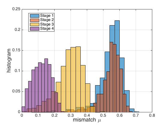
Figure 1: These are the mismatch histograms of the four follow-up searches, so the y-axis represents normalised counts. For a given search and search set-up, the mismatch distribution depends of the template grid. The injection-and-recovery Monte Carlo studies to determine these distributions were performed without noise.

The parameters for the various stages are summarised in Table 1. The grids in frequency and spindown are each described by a single parameter, the grid spacing, which is constant over the search range. The same frequency grid spacings are used for the coherent searches over the segments and for the incoherent summing. The spindown spacing for the incoherent summing step is finer than that used in for the coherent searches by a factor $\gamma$. The notation used here is consistent with that used in previous observational papers GalacticCenterSearch ; S6BucketStage0 ; S5GC1HF and in the GCT methods papers Pletsch:2008 ; Pletsch:2010 .

The sky grids for stages 1 to 4 are approximately uniform on the celestial sphere projected on the ecliptic plane. The tiling is an hexagonal covering of the unit circle with hexagons’ edge length $d$:

$$d(m_{\text{sky}})={1\over f}{{\sqrt{m_{\text{sky}}}}\over{\pi\tau_{E}}},$$ (1)

with $\tau_{E}\simeq 0.021$ s being half of the light travel time across the Earth and $m_{\text{sky}}$ the so-called mismatch parameter. As was done in previous searches FullS5EH ; S6BucketStage0 the sky-grids are constant over 10Hz bands and the spacings are the ones associated through Eq. 1 to the highest frequency in the range. The sky grid of stage 0 is the union of two grids: one is uniform on the celestial sphere after projection onto the equatorial plane and the tiling (in the equatorial plane) is approximately square with edge $d(0.3)$ from Eq.1; the other grid is limited to the equatorial region ($0\leq\alpha\leq 2\pi$ and $-0.5\leq\delta\leq 0.5$), with constant actual $\alpha$ and $\delta$ spacings equal to $d(0.3)$ – see Fig.1 of S6BucketStage0 . The reason for the equatorial “patching” with a denser sky grid is to improve the sensitivity of the search.

	$T_{coh}$	$N_{seg}$	$\delta f$	$\delta{\dot{f_{c}}}$	$\gamma$	$m_{\text{sky}}$
	hrs		Hz	Hz/s
Stage 0	60	90	$1.6\times 10^{-6}$	$5.8\times 10^{-11}$	230	0.3 + equatorial patch
Stage 1	60	90	$3.6\times 10^{-6}$	$1\times 10^{-10}$	230	0.0042
Stage 2	140	44	$2.0\times 10^{-6}$	$2.4\times 10^{-11}$	100	0.0004
Stage 3	140	44	$1.8\times 10^{-6}$	$2.1\times 10^{-11}$	100	$1\times 10^{-5}$
Stage 4	280	22	$1.9\times 10^{-7}$	$7.0\times 10^{-12}$	50	$4\times 10^{-7}$

Table 1: Search parameters for each of the semi-coherent stages.

After each stage a threshold is set on the detection statistic to determine what candidates will be searched by the next stage. We set this detection threshold to be the highest such that the weakest signal that survived the first stage of the pipeline would, with high confidence, not be lost.

The set-up for each stage is determined at fixed computation cost. The computational cost is mostly set by practical considerations such as the time-frame on which we’d like to have a result, the number of stages that we envision in the hierarchy and the availability of Einstein@Home.

Since an analytical model that predicts the sensitivity of a search with the current implementation of the GCT method does not exist, we consider different search set-ups and for every set-up we perform fake-signal injection and recovery Monte Carlos. From these we determine the detection efficiency and the signal parameter uncertainty for signals at the detection threshold. We pick the search set-up based on these. Typically the search setup with the lowest parameter uncertainty volume ($R$ given below) also has the highest detection efficiency and we pick that. As a further cross-check we also determine the mismatch distributions for the detection statistic. We define the mismatch $\mu$ as

$$\mu=\frac{2\overline{\mathcal{F}}_{\mathrm{signal}}-2\overline{\mathcal{F}}_{\mathrm{candidate}}}{2\overline{\mathcal{F}}_{\mathrm{signal}}-4}$$ (2)

where $\overline{\mathcal{F}}_{\mathrm{signal}}$ is the value of the detection statistic that we measure when we search the data with a template that is perfectly matched to the signal and $\overline{\mathcal{F}}_{\mathrm{candidate}}$ is the value of the detection statistic that we obtain when running a search on a set of templates none of which, in general, will perfectly coincide with the signal waveform. The mismatch is hence a measure of how fine the grid that we are using is. As expected, Fig. 1 shows that the grids of subsequent stages get finer and finer.

At each stage we determine the signal parameter uncertainty for signals at least at the detection threshold, in each search dimension: the distance in parameter space around a candidate that with high confidence (at least 90%), includes the signal parameter values. The uncertainty region around each candidate associated with stage $i$ is searched in stage $i+1$. The uncertainty volume at stage $i$ is smaller than the containment volume of stage $i-1$.

III The S6 search follow-up

A series of all-sky Einstein@Home  searches looked for signals with frequencies from 50 Hz through 510 Hz and frequency derivatives from $3.1\times 10^{-10}$ Hz/s through $-2.6\times 10^{-9}$ Hz/s. Results from these were combined and analysed as described in S6BucketStage0 : no significant candidate was found and upper limits were set on the gravitational wave signal amplitude in the target signal parameter space. The data set that we begin with, is that described in Section III.1 and III.2 of S6BucketStage0 : a ranked-list of $3.8\times 10^{10}$ candidates each with an associated detection statistic value $2\overline{\mathcal{F}}$. We now take the 16 million most promising regions in parameter space from that search and inspect them more closely. This is done in four stages which we describe in the next subsections.

We remind the reader that some of the input data to this search was treated by substituting the original frequency-domain data with fake Gaussian noise at the same level as that of the neighbouring frequencies. This is done in frequency regions affected by well-known artefacts, as described in S6BucketStage0 . Results stemming entirely from this fake data are not considered in any further stage. Moreover, after the initial Einstein@Home  search, the results in 50 mHz bands were visually inspected and those 50 mHz bands that present obvious noise disturbances are also removed from the analysis. A complete list of the excluded bands is given in the Appendixes of S6BucketStage0 . We will come back to this point as we present the results of this search.

III.1 Stage 0

This is the most complex stage of the hierarchy and determines the sensitivity of the search: if a signal does not pass this initial stage it will be lost forever. So we try here to keep the threshold that candidates have to exceed to be considered further as low as possible, compatibly with the feasibility of the next stage with the available computing resources. Such threshold was set at $2\overline{\mathcal{F}}=6.109$.

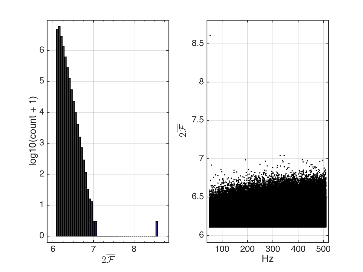
Figure 2: Candidates that are followed-up in stage 1 : the distribution of their detection statistic values $2\overline{\mathcal{F}}$ (left plot) and their distribution as a function of frequency (right plot).

The identification of correlated candidates saves compute cycles in the next steps of the search. As was done in GalacticCenterSearch the clustering procedure aims at bundling together candidates that could be ascribed to the same signal. In fact, a loud signal as well as a loud disturbance would produce high values of the detection statistic at a number of different template grid points and it would be a waste to follow up each of these independently. As described in GalacticCenterSearch ; GalacticCenterMethod we begin with the loudest candidate, i.e. the candidate with the highest value of $2\overline{\mathcal{F}}$ . This is the seed for the first cluster. We associate with it close-by candidates in parameter space. Together, the seed and the nearby candidates, constitute the first cluster. We remove the candidates from the first cluster from the candidate list. The loudest candidate on the resulting list is the seed of the second cluster. We proceed in the same way as for the first cluster and reiterate the procedure until no more seeds with $2\overline{\mathcal{F}}$ values equal to or larger than 6.109 remain.

Monte Carlo studies are conducted to determine the cluster box size, i.e. the neighbourhood of the seed that determines the cluster occupants. We inject signals in Gaussian noise data at the level of our detectors’ noise, search a small parameter space region around the signal parameters and use the resulting candidates as representative of what we would find in an actual search, after comparing them with the candidates obtained in the case of ’noise-only’. For signals at the detection threshold the 90% confidence cluster box is:

$$\begin{cases}\Delta f^{\text{ Stage-0}}&=\pm 1.2\times 10^{-3}{~{}\text{Hz}}\\ \Delta{\dot{f}}^{\text{ Stage-0}}&=\pm 2.6\times 10^{-10}{~{}\text{Hz/s}}\\ \Delta{\text{sky}}^{\text{ Stage-0}}&\simeq 25{\text{ points around seed}}\end{cases}$$ (3)

If we consider as cluster occupants only those with $2\overline{\mathcal{F}}$ values greater or equal to 5.9, we observe that signals tend to produce slight over-densities in the clusters with respect to noise. This feature is exploited with an occupancy veto that discards all clusters with less than 2 occupants. We find that the false dismissal for signals at threshold is hardly affected ($\sim$ 0.02% of signal clusters ) whereas the noise rejection is quite significant: we exclude 45% of signal clusters .

This same set of injection-data is utilised to characterise the false dismissals and the parameter uncertainty regions for all the stages of the hierarchy.

To summarise: the total number of candidates returned by the Einstein@Home  searches is $3.8\times 10^{10}$ . Of these we consider the ones with $2\overline{\mathcal{F}}$ above 6.109 , excluding frequency bands with obvious noise disturbances. There are 21.6 million such candidates. After clustering and occupancy veto we have reduced this number to 16.23 $\times 10^{6}$ . The distribution of the detection statistic values $2\overline{\mathcal{F}}$ for these candidates is shown in Fig. 2 as well as their distribution in frequency. The maximum value is 8.6 and occurs at $\sim$ 52 Hz. All remaining values are smaller than 7.1 .

III.2 Stage 1

In this stage we search a volume of parameter space (Eqs. 3) around each candidate (around each cluster seed) equal to the cluster box defined in 3. We fix the total run time to be 4 months on Einstein@Home  and this yields an optimal search set-up having the same coherent time baseline as stage 0, 60 hours, with the same number of segments $N_{seg}=90$ and the grid spacings shown in Table 1. We use the same ranking statistic as in the original search S6BucketStage0 , the $\widehat{O}_{{{\mathrm{{S}}}{\mathrm{{G}}{\mathrm{{L}}}}}}$ Keitel:2013 , with the same tunings. The 90% uncertainty regions for this search set-up for signals just above the detection threshold are

$$\begin{cases}\Delta f^{\text{ Stage-1}}&=\pm 6.7\times 10^{-4}{~{}\text{Hz}}\\ \Delta{\dot{f}}^{\text{ Stage-1}}&=\pm 1.8\times 10^{-10}{~{}\text{Hz/s}}\\ \Delta{\text{sky}}^{\text{ Stage-1}}&\simeq 0.55~{}\Delta{\text{sky}}^{\text{ Stage-0}}\end{cases}$$ (4)

The search is divided among 16.23 $\times 10^{6}$ work-units (WUs) each lasting about 2 hours and performed by one of the Einstein@Homevolunteer computers. From each follow-up search we record the most significant candidate. The distribution of these is shown in Fig.3. A threshold at $\overline{\mathcal{F}}=$ 6.109 has a $\sim$ 9% false dismissal for signals at threshold and a 70% noise rejection. Using this threshold to determine what candidates to consider in the next stage yields 5.3 $\times 10^{6}$ candidates.

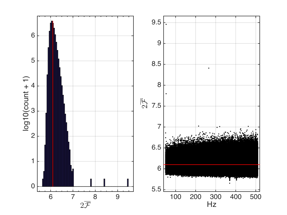
Figure 3: Loudest from each of the stage-1 searches: the distribution of their detection statistic values $2\overline{\mathcal{F}}$ (left plot) and their distribution as a function of frequency (right plot). The red line marks $2\overline{\mathcal{F}}=6.109$ which is the threshold at and above which candidates are passed on to stage-2.

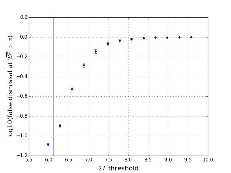
Figure 4: Fraction of signals that are recovered with a detection statistic value larger than or equal to the threshold value after the stage-1 follow-up.

III.3 Stage 2

In this stage we search a volume of parameter space around each candidate defined by Eq. 4. As shown in Table 1, we use a coherent time baseline which is about twice as long as that used in the previous stages and the grid spacings finer. The ranking statistic is $\widehat{O}_{{{\mathrm{{S}}}{\mathrm{{G}}{\mathrm{{L}}}}}}$ with the same tunings ($c_{*}$ and normalized SFT power threshold) as in the previous stages. The computational load is divided among 5.3 $\times 10^{6}$ WUs, each lasting about 12 hrs.

The $>$ 99% uncertainty regions for this search set-up for signals close to the detection threshold are

$$\begin{cases}\Delta f^{\text{ Stage-2}}&=\pm 1.9\times 10^{-4}{~{}\text{ Hz}}\\ \Delta{\dot{f}}^{\text{ Stage-2}}&=\pm 3.5\times 10^{-11}{~{}\text{Hz/s}}\\ \Delta{\text{sky}}^{\text{ Stage-2}}&\simeq 0.19~{}\Delta{\text{sky}}^{\text{ Stage-1}}\end{cases}$$ (5)

As done in stage 1 we record the most significant candidate from each search. The distribution is shown in Fig.5. In the next stage we follow-up the top 1.1 million candidates, corresponding to a threshold on $2\overline{\mathcal{F}}$ at 7.38 . This threshold has a $\sim$ 0.6% false dismissal for signals at threshold and a 79% noise rejection.

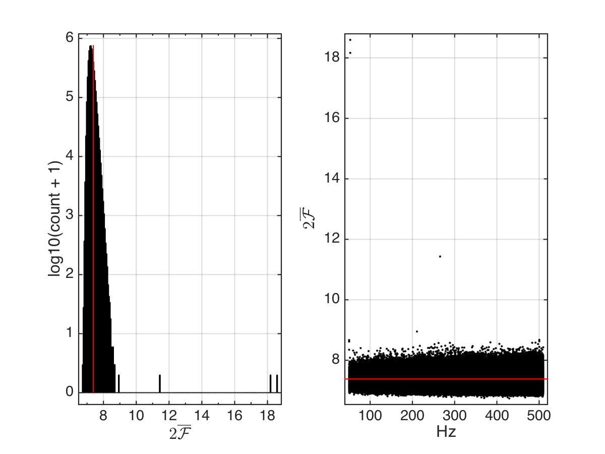
Figure 5: Loudest from each of the stage-2 searches: the distribution of their detection statistic values $2\overline{\mathcal{F}}$ (left plot) and their distribution as a function of frequency (right plot). The red line marks $2\overline{\mathcal{F}}=7.38$ which is the threshold at and above which candidates are passed on to stage-3.

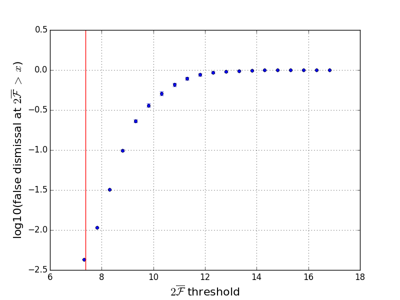
Figure 6: Fraction of signals that are recovered with a detection statistic value larger than or equal to the threshold value after the stage-2 follow-up.

III.4 Stage 3

In this stage we search a volume of parameter space around each candidate defined by Eq.5. As shown in Table 1, the coherent timebaseline is as long as that used in the previous stage but the grid spacings are finer. The search is divided among 1.1 million WUs each lasting about 2 hours.

The $>$ 99% uncertainty regions for this search set-up for signals close to the detection threshold are

$$\begin{cases}\Delta f^{\text{ Stage-3}}&=\pm 5\times 10^{-5}{~{}\text{Hz}}\\ \Delta{\dot{f}}^{\text{ Stage-3}}&=\pm 7\times 10^{-12}{~{}\text{Hz/s}}\\ \Delta{\text{sky}}^{\text{ Stage-3}}&\simeq 0.4~{}\Delta{\text{sky}}^{\text{ Stage-2}}\end{cases}$$ (6)

As done in previous stages we record the most significant candidate from each search. The distribution is shown in Fig.7. In the next stage we follow-up the top 10 candidates, corresponding to a threshold on $2\overline{\mathcal{F}}$ at 8.82 . This threshold has a $\sim 4\times 10^{-4}$ false dismissal for signals at threshold and a 99.9991% noise rejection.

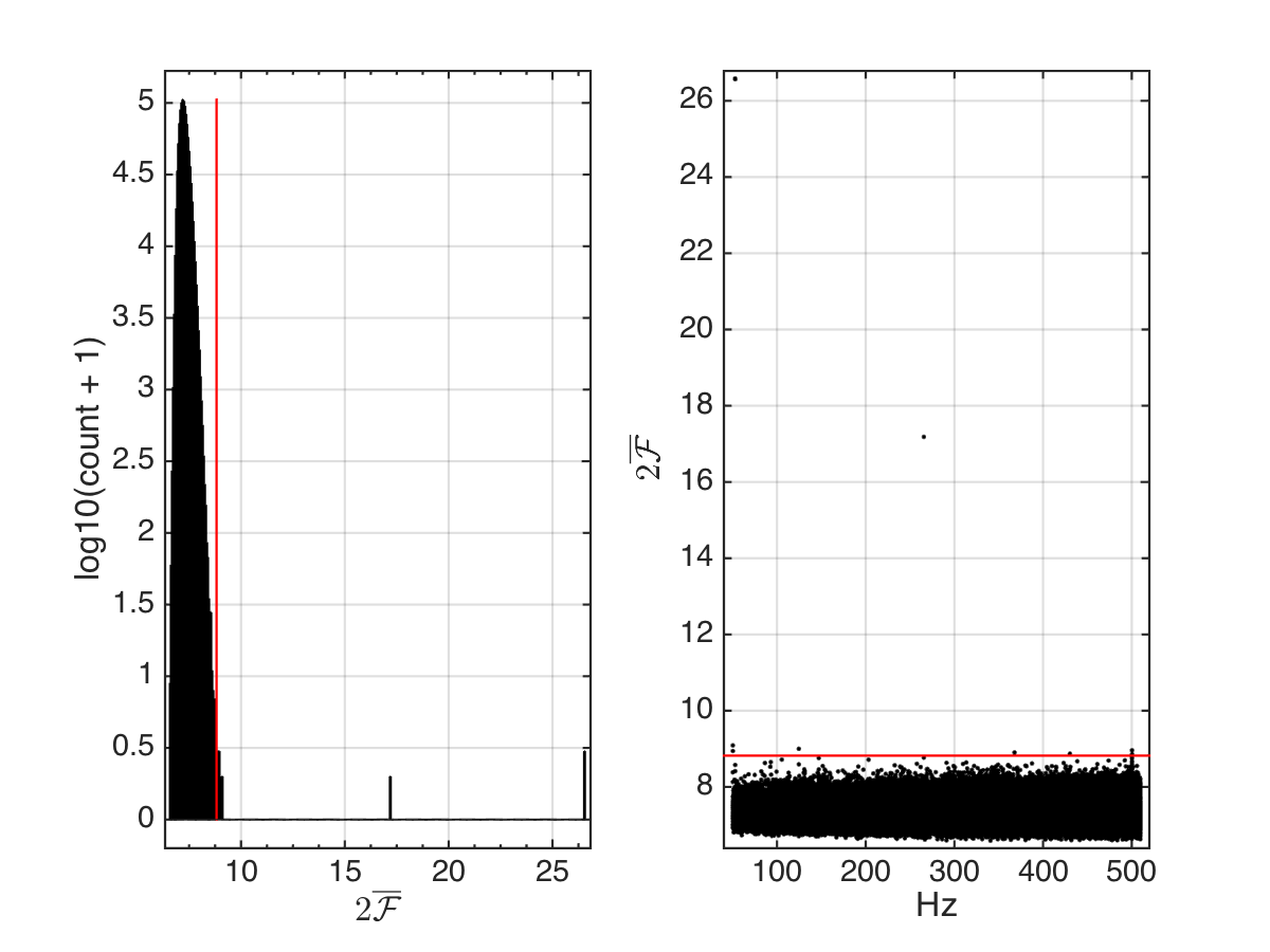
Figure 7: Loudest from each of the stage-3 searches: the distribution of their detection statistic values $2\overline{\mathcal{F}}$ (left plot) and their distribution as a function of frequency (right plot). The red line marks $2\overline{\mathcal{F}}=8.82$ which is the threshold at and above which candidates are passed on to stage-4.

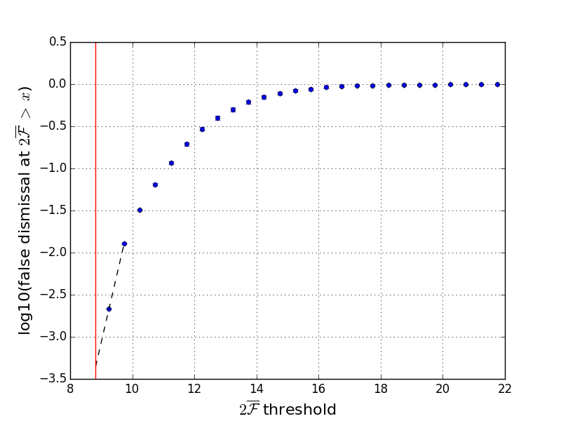
Figure 8: Fraction of signals that are recovered with a detection statistic value larger than or equal to the threshold value (vertical line) after the stage-3 follow-up. The dashed line is a linear extrapolation based on the last two data points to guide the eye to the false dismissal value for signals at threshold. This line is a conservative estimate in the sense that it over estimates the false dismissal.

III.5 Stage 4

In this stage we search a volume of parameter space around each candidate defined by Eq.7. The set-up of choice has a coherent time-baseline of 280 hrs, twice as long as that used in stage-3, and the grid spacings shown in Table 1. The search has a relatively modest cost and is performed on the Atlas cluster: each follow-up lasts about 14 hours. The ranking statistic is $\widehat{O}_{{{\mathrm{{S}}}{\mathrm{{G}}{\mathrm{{L}}}}}}$ with a re-tuned $c_{*}=96.1$. We consider the loudest candidate from each of the 10 follow-ups. In our Monte Carlo studies no signal candidate (out of 464 injections at threshold) is found more distant than:

$$\begin{cases}\Delta f^{\text{ Stage-4}}&=\pm 4\times 10^{-7}{~{}\text{Hz}}\\ \Delta{\dot{f}}^{\text{ Stage-4}}&=\pm 4.0\times 10^{-13}{~{}\text{Hz/s}}\\ \Delta{\text{sky}}^{\text{ Stage-4}}&\simeq 0.03~{}\Delta{\text{sky}}^{\text{ Stage-3}}\end{cases}$$ (7)

None of those injections has a $2\overline{\mathcal{F}}$ below 16.2. Conservatively, we pick a threshold at 15.0 . The Gaussian false alarm at $2\overline{\mathcal{F}}=$ 15.0 is very low ($\approx$ $2\times 10^{-20}$) and hence we do not expect any candidate from random Gaussian noise fluctuations.

Since we only follow-up 10 candidates we report our findings explicitly for each of them in Tab.2.

Candidates 3, 4 and 6 satisfy this condition but unfortunately they are ascribable to fake signals hardware-injected in the detector to test the detection pipelines. The search recovers all fake signals in the data with parameters within its search range and not absurdly loud. We note that candidates 3 and 4 come from the same fake signal. For a complete list of the fake signals present in the data – see Table 6 of S6NineYoungSNRs . In Table 3 we show the signal parameters and report the distance with respect to the candidate parameter values. These distances are all within the Stage-4 uncertainties of 7. We do not follow up these candidates any further because we know that they are associated with the hardware injections.

The remaining candidates are below the threshold of 15.0 which is the minimum value of $2\overline{\mathcal{F}}$ that we demand candidates to pass before we inspect them further.

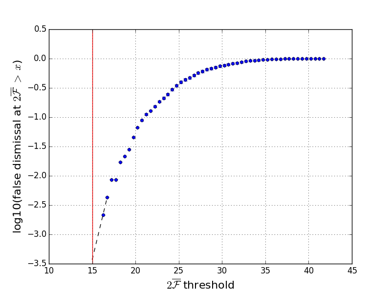
Figure 9: Fraction of signals that are recovered with a detection statistic value larger than or equal to the threshold value (vertical line) after the stage-4 follow-up. The dashed line is a linear extrapolation based on the last two data points to guide the eye to the false dismissal value for signals at threshold. This line is a conservative estimate in the sense that it over estimates the false dismissal.

ID	$f$ [Hz]	$\alpha$ [rad]	$\delta$ [rad]	${\dot{f}}$ [Hz/s]	$2\overline{\mathcal{F}}$	$2\overline{\mathcal{F}}_{\text{H1}}$	$2\overline{\mathcal{F}}_{\text{L1}}$
1	50.19985463	4.7716026	1.1412922	3.013 $\times 10^{-11}$	11.6	6.9	9.5
2	50.20001612	4.7124554	1.1683832	-5.674 $\times 10^{-12}$	12.3	5.5	11.2
3	52.80832455	5.2805366	-1.4631895	7.311 $\times 10^{-14}$	52.0	16.9	39.7
4	52.80832422	5.2819543	-1.4632398	2.968 $\times 10^{-14}$	55.9	18.1	44.0
5	124.60002077	4.7067880	1.1648704	-4.164 $\times 10^{-12}$	11.8	11.2	6.1
6	265.57623841	1.2487972	-0.9812202	-4.015 $\times 10^{-12}$	37.3	25.1	17.0
7	367.83543941	1.4807437	0.7112582	-9.236 $\times 10^{-10}$	10.4	9.5	4.9
8	430.28626637	6.1499768	0.9203753	-2.056 $\times 10^{-9}$	10.0	7.3	5.5
9	500.36312713	4.7121294	1.1617860	9.878 $\times 10^{-13}$	12.2	11.9	5.4
10	500.36594568	4.5662765	1.4276343	-2.507 $\times 10^{-9}$	10.6	10.0	4.6

Table 2: Stage-4 results from each of the 10 follow-ups from the candidates surviving Stage-3. For illustration purposes in the last two columns we show the values of the average single-detector detection statistics. Typically for signals the single-detector values do not exceed the multi-detector $2\overline{\mathcal{F}}$.

IV Results

ID	$f_{\text{s}}$ [Hz]	$\alpha_{\text{s}}$ [rad]	$\delta_{\text{s}}$ [rad]	$\dot{f_{\text{s}}}$ [Hz/s]	$\Delta f$ [Hz]	$\Delta\alpha$ [rad]	$\Delta\delta$ [rad]	$\Delta{\dot{f}}$ [Hz/s]
3	52.8083244	5.281831296	-1.463269033	-4.03 $\times 10^{-18}$	1.5 $\times 10^{-7}$	-1.29 $\times 10^{-3}$	7.95 $\times 10^{-5}$	7.3 $\times 10^{-14}$
4	52.8083244	5.281831296	-1.463269033	-4.03 $\times 10^{-18}$	-1.8 $\times 10^{-7}$	1.23 $\times 10^{-4}$	2.92 $\times 10^{-5}$	3.0 $\times 10^{-14}$
6	265.5762386	1.248816734	-0.981180225	-4.15 $\times 10^{-12}$	-1.9 $\times 10^{-7}$	-1.95 $\times 10^{-5}$	-4.00 $\times 10^{-5}$	1.4 $\times 10^{-13}$

Table 3: Columns 2-5 show the parameters of the fake injected signal closest to the candidate whose ID identifies it in Table 2. Columns 6-9 display the distance between the candidates’ and the signals’ parameters (candidate parameter minus signal parameter). The reference time eference time (GPS s): 960541454.5

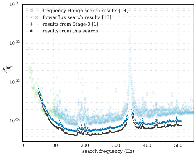
Figure 10: 90% confidence upper limits on the gravitational wave amplitude of continuous gravitational wave signals with frequency in 0.5 Hz bands and with spindown values within the searched range. The lowest set of points (black circles) are the results of this search. For comparison we show the upper limits from only the stage-0 results S6BucketStage0 . These lie on the curve above the lowest one and are marked by dark blue diamonds. The results from a previous broad all-sky survey S6Powerflux are the top curve (lighter circles and crosses) above 100 Hz. In the lower frequency we compare with a search on Virgo data contemporary to the LIGO S6 data AllSkyLowFreqVirgo .

The search did not reveal any continuous gravitational wave signal in the parameter volume that was searched. We hence set frequentist upper limits on the maximum gravitational wave amplitude consistent with this null result in $0.5$ Hz bands : $h_{0}^{90\%}$(f). $h_{0}^{90\%}$(f) is the GW amplitude such that 90% of a population of signals with parameter values in our search range would have been detected by our search, i.e. would have survived the last $2\overline{\mathcal{F}}$ threshold at 15.0 at stage-4. Since an actual full scale injection-and-recovery Monte Carlo for the entire set of follow-ups in every $0.5$ Hz band is prohibitive, in the same spirit as S6BucketStage0 ; S5GC1HF , we perform such study in a limited set of trial bands. We pick 100. For each of these we determine the sensitivity depth of the search corresponding to the detection criterion stated above. As representative of the sensitivity depth ${{\mathcal{D}}}^{90\%}$ of this hierarchical search, we take the average of these depths, 46.9 $[{1/\sqrt{\text{Hz}}}]$. Given the noise level of the data as a function of frequency, $S_{h}(f)$ , we then determine the 90% upper limits as

$${h{{}_{0}^{90\%}}(f)}={{\sqrt{S_{h}(f)}}\over{{{\mathcal{D}}}^{90\%}}}.$$ (8)

Figure 10 shows these upper limits as a function of frequency. They are also presented in tabular form in the Appendix with the associated uncertainties which amount to 20%, including calibration uncertainties. The most constraining upper limit is in the band between 170.5 and 171 Hz and it is 4.3 $\times 10^{-25}$. At the upper end of the frequency range, around 510 Hz, the upper limit rises to 7.6 $\times 10^{-25}$.

The upper limits can be recast as exclusion regions in the signal frequency-ellipticity plane parameterised by the distance, for an isolated source emitting continuous gravitational waves due to its shape presenting an ellipticity $\epsilon$

$$\epsilon={|{I_{xx}-I_{yy}}|\over I_{zz}}$$ (9)

where $I$ are the principal moments of inertia and the coordinate system is taken so that the $z$-axis is aligned with the spin axis of the star. Fig.11 shows these upper limits. Above 200 Hz we can exclude sources with ellipticities larger than $10^{-6}$ within 100 pc of Earth and above 400 Hz ellipticities above $4\times 10^{-7}$.

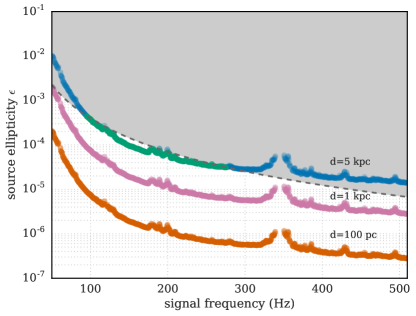
Figure 11: Ellipticity $\epsilon$ of a source at a distance d emitting continuous gravitational waves that would have been detected by this search. The dashed line shows the spin-down ellipticity for the highest magnitude spindown parameter value searched: 2.6 $\times 10^{-9}$ Hz/s. The spin-down ellipticity is the ellipticity necessary for all the lost rotational kinetic energy to be emitted in gravitational waves. If we assume that the observed spin-down is all actual spin-down of the object, then no ellipticities could be possible above the dashed curve. In reality the observed and actual spindown could differ due to radial motion of the source. In this case the actual spin-down of the object may even be larger than the apparent one. In this case our search would be sensitive to objects with ellipticities above the dashed line.

V Conclusions

With a hierarchy of five semi-coherent searches at increasing coherent time baselines and resolutions in parameter space we searched over 16 million regions in few hundred Hz around the most sensitive frequencies of the LIGO detectors during the S6 science run. All stages but the very last ran on the Einstein@Home  distributed computing project lasting a few to several weeks. This is the first large-scale hierarchical search for gravitational wave signals ever performed.

Having carried out this search proves that one can successfully perform deep follow-ups of marginal candidates and elevate their significance to the level necessary to be able to claim a detection. This paper proves that searches with thresholds at the level of the Einstein@Home  search described in Walsh:2016hyc are possible; Walsh:2016hyc demonstrates that they are the most sensitive and our observational results confirm this.

The sensitivity of broad surveys for continuous gravitational wave signals is computationally limited. For this reason we employ Einstein@Home  to deploy our searches. However, following up tens of millions of candidates is not just a matter of having the computational power. This paper illustrates how to perform and optimise the different stages, factoring in all the practical aspects of a real analysis.

None of the investigated candidates survived the five stages apart from those arising from the two fake signals injected in the detector for control purposes. These fake signals were recovered with the correct signal parameters. Candidate 6 comes from a hardware injection weak enough that no other search on this data set was ever able to detect it. This search recovers it well above the detection threshold.

The gravitational wave amplitude upper limits that we set improve on existing ones S6BucketStage0 by about $30\%$. This corresponds to an increase in accessible space volume of $\simeq 2$.

We excluded 10% of the original data from this analysis because the stage-0 results had different statistical properties than the bulk of the results and the automated methods employed here which are necessary in order to deal with a large number of candidates, would not have yielded meaningful statistical results. We might go back to these excluded parameter space regions and attempt to extract information. This is a time-consuming process and the odds of finding a signal versus the odds of missing one by not analysing more sensitive data might well indicate that we shouldn’t pursue this.

The optimal set-up for the various stages and the upper limits were determined at the expense of signal injection-and-recovery Monte Carlo studies. This is due to the fact that the implementation of a stack-slide search that we are using does not allow an analytical prediction of the sensitivity of a search with a given set-up (coherent segments and grid spacings). This major drawback will soon be overcome by a new implementation of stack-slide searches based on Wette:2016raf ; Wette:2015lfa ; Wette:2014tca ; Wette:2013wza . Such a search is being characterised and tuned at the time of writing and we hope to employ it in the context of our contributions to the LIGO Scientific Collaboration for searches on data from the next LIGO run (O2).

In principle we would like to carry out the entire hierarchy of stages on Einstein@Home. For this to happen two aspects of the search presented here need to be automated: the visual inspection and the follow-up stages. The first is underway S6CasA . The second will be significantly eased by the new stack-slide search that we alluded to, above.

VI Acknowledgments

Our sincere gratitude firstly goes to the Einstein@Home volunteers who have made these searches possible: thank you, thank you, thank you. Maria Alessandra Papa, Sinéad Walsh, Bruce Allen and Xavier Siemens gratefully acknowledge the support from $\mathrm{NSF\;PHY}$ Grant 1104902. All the tuning and preparatory computational work for this search was carried out on the $\mathrm{ATLAS}$ super-computing cluster at the Max-Planck-Institut für Gravitationsphysik/ Leibniz Universität Hannover. We also acknowledge the Continuous Wave Group of the LIGO Scientific Collaboration for useful discussions and Graham Woan for reviewing the manuscript on behalf of the Collaboration.

This document has been assigned LIGO Laboratory document number LIGO-P1600213.

Appendix A Tabular data

A.1 Upper limit values

Table 4: First frequency of each half Hz signal frequency band in which we set upper limits and upper limit value for that band.

$\boldsymbol{f}$ (in Hz)	$\boldsymbol{h_{0}^{90\%}\times 10^{25}}$		$\boldsymbol{f}$ (in Hz)	$\boldsymbol{h_{0}^{90\%}\times 10^{25}}$		$\boldsymbol{f}$ (in Hz)	$\boldsymbol{h_{0}^{90\%}\times 10^{25}}$		$\boldsymbol{f}$ (in Hz)	$\boldsymbol{h_{0}^{90\%}\times 10^{25}}$
50.063	54.1 $\pm$ 10.8		50.563	52.6 $\pm$ 10.5		51.063	53.3 $\pm$ 10.7		51.563	53.2 $\pm$ 10.6
52.063	51.5 $\pm$ 10.3		52.563	48.7 $\pm$ 9.7		53.063	45.4 $\pm$ 9.1		53.563	43.5 $\pm$ 8.7
54.063	43.5 $\pm$ 8.7		54.563	42.5 $\pm$ 8.5		55.063	42.9 $\pm$ 8.6		55.563	40.2 $\pm$ 8.0
56.063	40.1 $\pm$ 8.0		56.563	39.1 $\pm$ 7.8		57.063	37.4 $\pm$ 7.5		57.563	36.9 $\pm$ 7.4
58.063	37.1 $\pm$ 7.4		58.563	40.6 $\pm$ 8.1		61.063	33.8 $\pm$ 6.8		61.563	29.5 $\pm$ 5.9
62.063	28.8 $\pm$ 5.8		62.563	28.4 $\pm$ 5.7		63.063	27.9 $\pm$ 5.6		63.563	26.0 $\pm$ 5.2
64.063	24.1 $\pm$ 4.8		64.563	22.9 $\pm$ 4.6		65.063	22.8 $\pm$ 4.6		65.563	23.2 $\pm$ 4.6
66.063	21.8 $\pm$ 4.4		66.563	20.9 $\pm$ 4.2		67.063	20.9 $\pm$ 4.2		67.563	21.5 $\pm$ 4.3
68.063	20.3 $\pm$ 4.1		68.563	20.6 $\pm$ 4.1		69.063	19.6 $\pm$ 3.9		69.563	20.1 $\pm$ 4.0
70.063	19.4 $\pm$ 3.9		70.563	18.6 $\pm$ 3.7		71.063	17.9 $\pm$ 3.6		71.563	17.8 $\pm$ 3.6
72.063	17.8 $\pm$ 3.6		72.563	17.9 $\pm$ 3.6		73.063	17.3 $\pm$ 3.5		73.563	17.3 $\pm$ 3.5
74.063	16.2 $\pm$ 3.2		74.563	15.9 $\pm$ 3.2		75.063	15.2 $\pm$ 3.0		75.563	16.0 $\pm$ 3.2
76.063	15.0 $\pm$ 3.0		76.563	14.4 $\pm$ 2.9		77.063	14.3 $\pm$ 2.9		77.563	14.2 $\pm$ 2.8
78.063	14.8 $\pm$ 3.0		78.563	13.7 $\pm$ 2.7		79.063	13.4 $\pm$ 2.7		79.563	14.3 $\pm$ 2.9
80.063	14.2 $\pm$ 2.8		80.563	13.3 $\pm$ 2.7		81.063	14.7 $\pm$ 2.9		81.563	12.9 $\pm$ 2.6
82.063	12.2 $\pm$ 2.4		82.563	11.9 $\pm$ 2.4		83.063	11.6 $\pm$ 2.3		83.563	11.3 $\pm$ 2.3
84.063	11.2 $\pm$ 2.2		84.563	11.0 $\pm$ 2.2		85.063	10.8 $\pm$ 2.2		85.563	10.8 $\pm$ 2.2
86.063	10.7 $\pm$ 2.1		86.563	10.9 $\pm$ 2.2		87.063	10.2 $\pm$ 2.0		87.563	10.1 $\pm$ 2.0
88.063	9.9 $\pm$ 2.0		88.563	10.0 $\pm$ 2.0		89.063	9.7 $\pm$ 1.9		89.563	9.7 $\pm$ 1.9
90.063	9.5 $\pm$ 1.9		90.563	9.4 $\pm$ 1.9		91.063	9.3 $\pm$ 1.9		91.563	9.2 $\pm$ 1.8
92.063	9.0 $\pm$ 1.8		92.563	8.9 $\pm$ 1.8		93.063	8.8 $\pm$ 1.8		93.563	8.8 $\pm$ 1.8
94.063	8.7 $\pm$ 1.7		94.563	8.6 $\pm$ 1.7		95.063	8.5 $\pm$ 1.7		95.563	8.3 $\pm$ 1.7
96.063	8.3 $\pm$ 1.7		96.563	8.2 $\pm$ 1.6		97.063	8.2 $\pm$ 1.6		97.563	8.1 $\pm$ 1.6
98.063	8.1 $\pm$ 1.6		98.563	8.1 $\pm$ 1.6		99.063	7.9 $\pm$ 1.6		99.563	7.8 $\pm$ 1.6
100.063	8.1 $\pm$ 1.6		100.563	7.8 $\pm$ 1.6		101.063	7.7 $\pm$ 1.5		101.563	7.5 $\pm$ 1.5
102.063	7.6 $\pm$ 1.5		102.563	7.4 $\pm$ 1.5		103.063	7.2 $\pm$ 1.4		103.563	7.1 $\pm$ 1.4
104.063	7.2 $\pm$ 1.4		104.563	7.3 $\pm$ 1.5		105.063	7.2 $\pm$ 1.4		105.563	7.1 $\pm$ 1.4
106.063	7.3 $\pm$ 1.5		106.563	7.1 $\pm$ 1.4		107.063	7.0 $\pm$ 1.4		107.563	7.3 $\pm$ 1.5
108.063	7.3 $\pm$ 1.5		108.563	6.8 $\pm$ 1.4		109.063	6.8 $\pm$ 1.4		109.563	6.7 $\pm$ 1.3
110.063	6.7 $\pm$ 1.3		110.563	6.7 $\pm$ 1.3		111.063	6.8 $\pm$ 1.4		111.563	6.9 $\pm$ 1.4
112.063	6.7 $\pm$ 1.3		112.563	6.6 $\pm$ 1.3		113.063	7.1 $\pm$ 1.4		113.563	6.6 $\pm$ 1.3
114.063	6.4 $\pm$ 1.3		114.563	6.4 $\pm$ 1.3		115.063	6.3 $\pm$ 1.3		115.563	6.2 $\pm$ 1.2
116.063	6.4 $\pm$ 1.3		116.563	6.8 $\pm$ 1.4		117.063	6.8 $\pm$ 1.4		117.563	6.8 $\pm$ 1.4
118.063	7.9 $\pm$ 1.6		118.563	6.9 $\pm$ 1.4		121.063	7.0 $\pm$ 1.4		121.563	6.3 $\pm$ 1.3
122.063	6.5 $\pm$ 1.3		122.563	6.5 $\pm$ 1.3		123.063	6.6 $\pm$ 1.3		123.563	6.4 $\pm$ 1.3
124.063	6.1 $\pm$ 1.2		124.563	5.9 $\pm$ 1.2		125.063	5.9 $\pm$ 1.2		125.563	6.3 $\pm$ 1.3
126.063	6.1 $\pm$ 1.2		126.563	6.5 $\pm$ 1.3		127.063	6.0 $\pm$ 1.2		127.563	6.0 $\pm$ 1.2
128.063	5.8 $\pm$ 1.2		128.563	6.2 $\pm$ 1.2		129.063	6.1 $\pm$ 1.2		129.563	6.3 $\pm$ 1.3
130.063	6.0 $\pm$ 1.2		130.563	6.1 $\pm$ 1.2		131.063	5.6 $\pm$ 1.1		131.563	5.4 $\pm$ 1.1
132.063	5.4 $\pm$ 1.1		132.563	5.3 $\pm$ 1.1		133.063	5.3 $\pm$ 1.1		133.563	5.2 $\pm$ 1.0
134.063	5.0 $\pm$ 1.0		134.563	5.0 $\pm$ 1.0		135.063	5.0 $\pm$ 1.0		135.563	5.0 $\pm$ 1.0
136.063	5.0 $\pm$ 1.0		136.563	4.9 $\pm$ 1.0		137.063	5.0 $\pm$ 1.0		137.563	5.0 $\pm$ 1.0
138.063	4.9 $\pm$ 1.0		138.563	4.9 $\pm$ 1.0		139.063	5.1 $\pm$ 1.0		139.563	4.9 $\pm$ 1.0
140.063	4.9 $\pm$ 1.0		140.563	4.9 $\pm$ 1.0		141.063	4.8 $\pm$ 1.0		141.563	5.0 $\pm$ 1.0
142.063	4.8 $\pm$ 1.0		142.563	4.8 $\pm$ 1.0		143.063	4.8 $\pm$ 1.0		143.563	4.8 $\pm$ 1.0
144.063	4.9 $\pm$ 1.0		144.563	4.8 $\pm$ 1.0		145.563	4.6 $\pm$ 0.9		146.063	4.6 $\pm$ 0.9
146.563	4.6 $\pm$ 0.9		147.063	4.6 $\pm$ 0.9		147.563	4.6 $\pm$ 0.9		148.063	4.6 $\pm$ 0.9
148.563	4.6 $\pm$ 0.9		149.063	4.5 $\pm$ 0.9		149.563	4.5 $\pm$ 0.9		150.063	4.5 $\pm$ 0.9
150.563	4.5 $\pm$ 0.9		151.063	4.5 $\pm$ 0.9		151.563	4.5 $\pm$ 0.9		152.063	4.5 $\pm$ 0.9
152.563	4.5 $\pm$ 0.9		153.063	4.6 $\pm$ 0.9		153.563	4.5 $\pm$ 0.9		154.063	4.5 $\pm$ 0.9
154.563	4.5 $\pm$ 0.9		155.063	4.6 $\pm$ 0.9		155.563	4.5 $\pm$ 0.9		156.063	4.5 $\pm$ 0.9
156.563	4.5 $\pm$ 0.9		157.063	4.5 $\pm$ 0.9		157.563	4.5 $\pm$ 0.9		158.063	4.5 $\pm$ 0.9
158.563	4.5 $\pm$ 0.9		159.063	4.5 $\pm$ 0.9		159.563	4.4 $\pm$ 0.9		160.063	4.4 $\pm$ 0.9
160.563	4.5 $\pm$ 0.9		161.063	4.5 $\pm$ 0.9		161.563	4.4 $\pm$ 0.9		162.063	4.5 $\pm$ 0.9
162.563	4.5 $\pm$ 0.9		163.063	4.5 $\pm$ 0.9		163.563	4.5 $\pm$ 0.9		164.063	4.4 $\pm$ 0.9
164.563	4.4 $\pm$ 0.9		165.063	4.4 $\pm$ 0.9		165.563	4.4 $\pm$ 0.9		166.063	4.4 $\pm$ 0.9
166.563	4.4 $\pm$ 0.9		167.063	4.4 $\pm$ 0.9		167.563	4.4 $\pm$ 0.9		168.063	4.3 $\pm$ 0.9
168.563	4.3 $\pm$ 0.9		169.063	4.3 $\pm$ 0.9		169.563	4.3 $\pm$ 0.9		170.063	4.3 $\pm$ 0.9
170.563	4.3 $\pm$ 0.9		171.063	4.3 $\pm$ 0.9		171.563	4.3 $\pm$ 0.9		172.063	4.3 $\pm$ 0.9
172.563	4.3 $\pm$ 0.9		173.063	4.3 $\pm$ 0.9		173.563	4.3 $\pm$ 0.9		174.063	4.4 $\pm$ 0.9
174.563	4.3 $\pm$ 0.9		175.063	4.4 $\pm$ 0.9		175.563	4.4 $\pm$ 0.9		176.063	4.8 $\pm$ 1.0
176.563	5.0 $\pm$ 1.0		177.063	5.0 $\pm$ 1.0		177.563	5.0 $\pm$ 1.0		178.063	5.1 $\pm$ 1.0
178.563	5.6 $\pm$ 1.1		181.063	5.7 $\pm$ 1.1		181.563	5.3 $\pm$ 1.1		182.063	5.3 $\pm$ 1.1
182.563	5.4 $\pm$ 1.1		183.063	5.2 $\pm$ 1.0		183.563	4.9 $\pm$ 1.0		184.063	5.1 $\pm$ 1.0
184.563	4.8 $\pm$ 1.0		185.063	5.0 $\pm$ 1.0		185.563	4.9 $\pm$ 1.0		186.063	4.9 $\pm$ 1.0
186.563	4.8 $\pm$ 1.0		187.063	4.8 $\pm$ 1.0		187.563	5.0 $\pm$ 1.0		188.063	5.3 $\pm$ 1.1
188.563	5.3 $\pm$ 1.1		189.063	6.3 $\pm$ 1.3		189.563	6.1 $\pm$ 1.2		190.063	5.5 $\pm$ 1.1
190.563	5.1 $\pm$ 1.0		191.063	4.8 $\pm$ 1.0		191.563	4.8 $\pm$ 1.0		192.063	4.8 $\pm$ 1.0
192.563	4.8 $\pm$ 1.0		193.063	4.6 $\pm$ 0.9		193.563	4.5 $\pm$ 0.9		194.063	4.7 $\pm$ 0.9
194.563	4.5 $\pm$ 0.9		195.063	4.8 $\pm$ 1.0		195.563	4.9 $\pm$ 1.0		196.063	5.1 $\pm$ 1.0
196.563	5.0 $\pm$ 1.0		197.063	4.9 $\pm$ 1.0		197.563	5.2 $\pm$ 1.0		198.063	5.3 $\pm$ 1.1
198.563	5.3 $\pm$ 1.1		199.063	6.2 $\pm$ 1.2		199.563	6.7 $\pm$ 1.3		200.063	5.6 $\pm$ 1.1
200.563	5.7 $\pm$ 1.1		201.063	5.9 $\pm$ 1.2		201.563	5.3 $\pm$ 1.1		202.063	5.3 $\pm$ 1.1
202.563	5.4 $\pm$ 1.1		203.063	4.9 $\pm$ 1.0		203.563	4.5 $\pm$ 0.9		204.063	4.4 $\pm$ 0.9
204.563	4.4 $\pm$ 0.9		205.063	4.4 $\pm$ 0.9		205.563	4.5 $\pm$ 0.9		206.063	4.4 $\pm$ 0.9
206.563	4.5 $\pm$ 0.9		207.063	4.6 $\pm$ 0.9		207.563	4.6 $\pm$ 0.9		208.063	4.9 $\pm$ 1.0
208.563	5.1 $\pm$ 1.0		209.063	5.0 $\pm$ 1.0		209.563	5.1 $\pm$ 1.0		210.063	5.1 $\pm$ 1.0
210.563	4.6 $\pm$ 0.9		211.063	4.6 $\pm$ 0.9		211.563	4.5 $\pm$ 0.9		212.063	4.4 $\pm$ 0.9
212.563	4.4 $\pm$ 0.9		213.063	4.5 $\pm$ 0.9		213.563	4.5 $\pm$ 0.9		214.063	4.3 $\pm$ 0.9
214.563	4.4 $\pm$ 0.9		215.063	4.4 $\pm$ 0.9		215.563	4.3 $\pm$ 0.9		216.063	4.3 $\pm$ 0.9
216.563	4.3 $\pm$ 0.9		217.063	4.3 $\pm$ 0.9		217.563	4.3 $\pm$ 0.9		218.063	4.3 $\pm$ 0.9
218.563	4.3 $\pm$ 0.9		219.063	4.4 $\pm$ 0.9		219.563	4.3 $\pm$ 0.9		220.063	4.4 $\pm$ 0.9
220.563	4.4 $\pm$ 0.9		221.063	4.4 $\pm$ 0.9		221.563	4.4 $\pm$ 0.9		222.063	4.5 $\pm$ 0.9
222.563	4.6 $\pm$ 0.9		223.063	4.7 $\pm$ 0.9		223.563	4.8 $\pm$ 1.0		224.063	4.7 $\pm$ 0.9
224.563	4.6 $\pm$ 0.9		225.063	4.6 $\pm$ 0.9		225.563	4.6 $\pm$ 0.9		226.063	4.5 $\pm$ 0.9
226.563	4.5 $\pm$ 0.9		227.063	4.5 $\pm$ 0.9		227.563	4.5 $\pm$ 0.9		228.063	4.5 $\pm$ 0.9
228.563	4.6 $\pm$ 0.9		229.063	4.6 $\pm$ 0.9		229.563	4.6 $\pm$ 0.9		230.063	4.9 $\pm$ 1.0
230.563	4.6 $\pm$ 0.9		231.063	4.6 $\pm$ 0.9		231.563	4.6 $\pm$ 0.9		232.063	4.5 $\pm$ 0.9
232.563	4.6 $\pm$ 0.9		233.063	4.7 $\pm$ 0.9		233.563	4.8 $\pm$ 1.0		234.063	4.7 $\pm$ 0.9
234.563	4.6 $\pm$ 0.9		235.063	4.6 $\pm$ 0.9		235.563	4.6 $\pm$ 0.9		236.063	4.5 $\pm$ 0.9
236.563	4.5 $\pm$ 0.9		237.063	4.5 $\pm$ 0.9		237.563	4.5 $\pm$ 0.9		238.063	4.5 $\pm$ 0.9
238.563	4.5 $\pm$ 0.9		240.563	4.6 $\pm$ 0.9		241.063	4.6 $\pm$ 0.9		241.563	4.7 $\pm$ 0.9
242.063	4.6 $\pm$ 0.9		242.563	4.5 $\pm$ 0.9		243.063	4.7 $\pm$ 0.9		243.563	4.7 $\pm$ 0.9
244.063	4.5 $\pm$ 0.9		244.563	4.5 $\pm$ 0.9		245.063	4.5 $\pm$ 0.9		245.563	4.6 $\pm$ 0.9
246.063	4.6 $\pm$ 0.9		246.563	4.6 $\pm$ 0.9		247.063	4.6 $\pm$ 0.9		247.563	4.6 $\pm$ 0.9
248.063	4.6 $\pm$ 0.9		248.563	4.7 $\pm$ 0.9		249.063	4.7 $\pm$ 0.9		249.563	4.6 $\pm$ 0.9
250.063	4.6 $\pm$ 0.9		250.563	4.6 $\pm$ 0.9		251.063	4.6 $\pm$ 0.9		251.563	4.6 $\pm$ 0.9
252.063	4.6 $\pm$ 0.9		252.563	4.6 $\pm$ 0.9		253.063	4.6 $\pm$ 0.9		253.563	4.6 $\pm$ 0.9
254.063	4.6 $\pm$ 0.9		254.563	4.6 $\pm$ 0.9		255.063	4.6 $\pm$ 0.9		255.563	4.8 $\pm$ 1.0
256.063	4.7 $\pm$ 0.9		256.563	4.7 $\pm$ 0.9		257.063	5.2 $\pm$ 1.0		257.563	4.8 $\pm$ 1.0
258.063	4.9 $\pm$ 1.0		258.563	4.8 $\pm$ 1.0		259.063	4.7 $\pm$ 0.9		259.563	4.7 $\pm$ 0.9
260.063	4.7 $\pm$ 0.9		260.563	4.7 $\pm$ 0.9		261.063	4.7 $\pm$ 0.9		261.563	4.7 $\pm$ 0.9
262.063	4.7 $\pm$ 0.9		262.563	4.7 $\pm$ 0.9		263.063	4.7 $\pm$ 0.9		263.563	4.7 $\pm$ 0.9
264.063	4.8 $\pm$ 1.0		264.563	4.8 $\pm$ 1.0		265.063	4.8 $\pm$ 1.0		265.563	4.8 $\pm$ 1.0
266.063	4.8 $\pm$ 1.0		266.563	4.8 $\pm$ 1.0		267.063	4.8 $\pm$ 1.0		267.563	5.0 $\pm$ 1.0
268.063	5.0 $\pm$ 1.0		268.563	4.9 $\pm$ 1.0		269.063	4.9 $\pm$ 1.0		269.563	4.9 $\pm$ 1.0
270.063	5.1 $\pm$ 1.0		270.563	5.2 $\pm$ 1.0		271.063	5.0 $\pm$ 1.0		271.563	5.0 $\pm$ 1.0
272.063	4.9 $\pm$ 1.0		272.563	4.9 $\pm$ 1.0		273.063	5.0 $\pm$ 1.0		273.563	5.0 $\pm$ 1.0
274.063	4.9 $\pm$ 1.0		274.563	4.9 $\pm$ 1.0		275.063	4.9 $\pm$ 1.0		275.563	5.0 $\pm$ 1.0
276.063	5.3 $\pm$ 1.1		276.563	5.1 $\pm$ 1.0		277.063	5.1 $\pm$ 1.0		277.563	5.2 $\pm$ 1.0
278.063	5.2 $\pm$ 1.0		278.563	5.2 $\pm$ 1.0		279.063	5.4 $\pm$ 1.1		279.563	5.7 $\pm$ 1.1
280.063	5.5 $\pm$ 1.1		280.563	5.4 $\pm$ 1.1		281.063	5.3 $\pm$ 1.1		281.563	5.6 $\pm$ 1.1
282.063	5.4 $\pm$ 1.1		282.563	5.3 $\pm$ 1.1		283.063	5.3 $\pm$ 1.1		283.563	5.5 $\pm$ 1.1
284.063	5.2 $\pm$ 1.0		284.563	5.2 $\pm$ 1.0		285.063	5.2 $\pm$ 1.0		285.563	5.1 $\pm$ 1.0
286.063	5.1 $\pm$ 1.0		286.563	5.2 $\pm$ 1.0		287.063	5.2 $\pm$ 1.0		287.563	5.2 $\pm$ 1.0
288.063	5.2 $\pm$ 1.0		288.563	5.3 $\pm$ 1.1		289.063	5.2 $\pm$ 1.0		289.563	5.2 $\pm$ 1.0
290.063	5.2 $\pm$ 1.0		290.563	5.2 $\pm$ 1.0		291.063	5.2 $\pm$ 1.0		291.563	5.2 $\pm$ 1.0
292.063	5.2 $\pm$ 1.0		292.563	5.2 $\pm$ 1.0		293.063	5.2 $\pm$ 1.0		293.563	5.2 $\pm$ 1.0
294.063	5.3 $\pm$ 1.1		294.563	5.2 $\pm$ 1.0		295.063	5.2 $\pm$ 1.0		295.563	5.2 $\pm$ 1.0
296.063	5.2 $\pm$ 1.0		296.563	5.3 $\pm$ 1.1		297.063	5.3 $\pm$ 1.1		297.563	5.3 $\pm$ 1.1
298.063	5.3 $\pm$ 1.1		298.563	5.3 $\pm$ 1.1		300.563	5.4 $\pm$ 1.1		301.063	5.4 $\pm$ 1.1
301.563	5.4 $\pm$ 1.1		302.063	5.5 $\pm$ 1.1		302.563	5.4 $\pm$ 1.1		303.063	5.5 $\pm$ 1.1
303.563	5.6 $\pm$ 1.1		304.063	5.5 $\pm$ 1.1		304.563	5.4 $\pm$ 1.1		305.063	5.5 $\pm$ 1.1
305.563	5.5 $\pm$ 1.1		306.063	5.6 $\pm$ 1.1		306.563	5.6 $\pm$ 1.1		307.063	5.5 $\pm$ 1.1
307.563	5.5 $\pm$ 1.1		308.063	5.5 $\pm$ 1.1		308.563	5.6 $\pm$ 1.1		309.063	5.7 $\pm$ 1.1
309.563	5.8 $\pm$ 1.2		310.063	5.7 $\pm$ 1.1		310.563	5.7 $\pm$ 1.1		311.063	5.7 $\pm$ 1.1
311.563	5.9 $\pm$ 1.2		312.063	5.8 $\pm$ 1.2		312.563	5.7 $\pm$ 1.1		313.063	5.7 $\pm$ 1.1
313.563	5.8 $\pm$ 1.2		314.063	5.8 $\pm$ 1.2		314.563	5.7 $\pm$ 1.1		315.063	5.8 $\pm$ 1.2
315.563	5.8 $\pm$ 1.2		316.063	5.9 $\pm$ 1.2		316.563	6.1 $\pm$ 1.2		317.063	6.0 $\pm$ 1.2
317.563	5.9 $\pm$ 1.2		318.063	6.0 $\pm$ 1.2		318.563	6.0 $\pm$ 1.2		319.063	6.0 $\pm$ 1.2
319.563	6.0 $\pm$ 1.2		320.063	6.0 $\pm$ 1.2		320.563	6.1 $\pm$ 1.2		321.063	6.2 $\pm$ 1.2
321.563	6.3 $\pm$ 1.3		322.063	6.6 $\pm$ 1.3		322.563	6.5 $\pm$ 1.3		323.063	6.8 $\pm$ 1.4
323.563	6.9 $\pm$ 1.4		324.063	7.0 $\pm$ 1.4		324.563	6.8 $\pm$ 1.4		325.063	6.9 $\pm$ 1.4
325.563	7.0 $\pm$ 1.4		326.063	7.2 $\pm$ 1.4		326.563	7.6 $\pm$ 1.5		327.063	7.9 $\pm$ 1.6
327.563	7.9 $\pm$ 1.6		328.063	7.8 $\pm$ 1.6		328.563	7.7 $\pm$ 1.5		329.063	7.5 $\pm$ 1.5
329.563	7.4 $\pm$ 1.5		330.063	7.7 $\pm$ 1.5		330.563	7.9 $\pm$ 1.6		331.063	7.7 $\pm$ 1.5
331.563	8.0 $\pm$ 1.6		332.063	8.0 $\pm$ 1.6		332.563	8.0 $\pm$ 1.6		333.063	8.1 $\pm$ 1.6
333.563	8.5 $\pm$ 1.7		334.063	9.1 $\pm$ 1.8		334.563	10.2 $\pm$ 2.0		335.063	11.0 $\pm$ 2.2
335.563	10.8 $\pm$ 2.2		336.063	10.8 $\pm$ 2.2		336.563	10.8 $\pm$ 2.2		337.063	10.9 $\pm$ 2.2
337.563	11.1 $\pm$ 2.2		338.063	11.6 $\pm$ 2.3		338.563	12.4 $\pm$ 2.5		339.063	13.4 $\pm$ 2.7
350.563	15.1 $\pm$ 3.0		351.063	13.6 $\pm$ 2.7		351.563	12.7 $\pm$ 2.5		352.063	12.9 $\pm$ 2.6
352.563	12.0 $\pm$ 2.4		353.063	12.1 $\pm$ 2.4		353.563	12.6 $\pm$ 2.5		354.063	11.3 $\pm$ 2.3
354.563	11.3 $\pm$ 2.3		355.063	13.1 $\pm$ 2.6		355.563	14.8 $\pm$ 3.0		356.063	14.4 $\pm$ 2.9
356.563	12.4 $\pm$ 2.5		357.063	10.2 $\pm$ 2.0		357.563	9.1 $\pm$ 1.8		358.063	9.4 $\pm$ 1.9
358.563	8.8 $\pm$ 1.8		361.063	7.6 $\pm$ 1.5		361.563	7.3 $\pm$ 1.5		362.063	7.2 $\pm$ 1.4
362.563	7.2 $\pm$ 1.4		363.063	8.1 $\pm$ 1.6		363.563	8.3 $\pm$ 1.7		364.063	8.2 $\pm$ 1.6
364.563	8.4 $\pm$ 1.7		365.063	7.1 $\pm$ 1.4		365.563	6.9 $\pm$ 1.4		366.063	7.0 $\pm$ 1.4
366.563	6.9 $\pm$ 1.4		367.063	7.2 $\pm$ 1.4		367.563	7.1 $\pm$ 1.4		368.063	6.8 $\pm$ 1.4
368.563	6.9 $\pm$ 1.4		369.063	6.7 $\pm$ 1.3		369.563	7.0 $\pm$ 1.4		370.063	7.1 $\pm$ 1.4
370.563	6.9 $\pm$ 1.4		371.063	7.5 $\pm$ 1.5		371.563	6.8 $\pm$ 1.4		372.063	6.4 $\pm$ 1.3
372.563	6.4 $\pm$ 1.3		373.063	6.5 $\pm$ 1.3		373.563	6.9 $\pm$ 1.4		374.063	7.3 $\pm$ 1.5
374.563	6.9 $\pm$ 1.4		375.063	7.2 $\pm$ 1.4		375.563	6.8 $\pm$ 1.4		376.063	6.7 $\pm$ 1.3
376.563	6.8 $\pm$ 1.4		377.063	7.7 $\pm$ 1.5		377.563	8.3 $\pm$ 1.7		378.063	7.1 $\pm$ 1.4
378.563	6.6 $\pm$ 1.3		379.063	6.5 $\pm$ 1.3		379.563	6.6 $\pm$ 1.3		380.063	6.6 $\pm$ 1.3
380.563	6.5 $\pm$ 1.3		381.063	6.6 $\pm$ 1.3		381.563	6.7 $\pm$ 1.3		382.063	6.8 $\pm$ 1.4
382.563	7.0 $\pm$ 1.4		383.063	7.3 $\pm$ 1.5		383.563	7.2 $\pm$ 1.4		384.063	7.4 $\pm$ 1.5
384.563	7.8 $\pm$ 1.6		385.063	8.1 $\pm$ 1.6		385.563	9.3 $\pm$ 1.9		386.063	8.9 $\pm$ 1.8
386.563	7.4 $\pm$ 1.5		387.063	7.0 $\pm$ 1.4		387.563	6.8 $\pm$ 1.4		388.063	6.9 $\pm$ 1.4
388.563	7.4 $\pm$ 1.5		389.063	6.9 $\pm$ 1.4		389.563	6.6 $\pm$ 1.3		390.063	6.5 $\pm$ 1.3
390.563	6.8 $\pm$ 1.4		391.063	7.0 $\pm$ 1.4		391.563	6.8 $\pm$ 1.4		392.063	6.6 $\pm$ 1.3
392.563	6.6 $\pm$ 1.3		393.063	6.6 $\pm$ 1.3		393.563	6.5 $\pm$ 1.3		394.063	6.5 $\pm$ 1.3
394.563	6.4 $\pm$ 1.3		395.063	6.5 $\pm$ 1.3		395.563	7.1 $\pm$ 1.4		396.063	6.8 $\pm$ 1.4
396.563	6.6 $\pm$ 1.3		397.063	6.6 $\pm$ 1.3		397.563	6.4 $\pm$ 1.3		398.063	6.4 $\pm$ 1.3
398.563	6.6 $\pm$ 1.3		399.063	6.6 $\pm$ 1.3		399.563	6.7 $\pm$ 1.3		400.563	6.6 $\pm$ 1.3
401.063	6.4 $\pm$ 1.3		401.563	6.4 $\pm$ 1.3		402.063	6.4 $\pm$ 1.3		402.563	6.4 $\pm$ 1.3
403.063	6.7 $\pm$ 1.3		403.563	6.8 $\pm$ 1.4		404.063	6.7 $\pm$ 1.3		404.563	6.5 $\pm$ 1.3
405.063	6.4 $\pm$ 1.3		405.563	6.6 $\pm$ 1.3		406.063	6.7 $\pm$ 1.3		406.563	6.5 $\pm$ 1.3
407.063	6.4 $\pm$ 1.3		407.563	6.4 $\pm$ 1.3		408.063	6.4 $\pm$ 1.3		408.563	6.5 $\pm$ 1.3
409.063	6.5 $\pm$ 1.3		409.563	6.4 $\pm$ 1.3		410.063	6.4 $\pm$ 1.3		410.563	6.5 $\pm$ 1.3
411.063	6.6 $\pm$ 1.3		411.563	6.6 $\pm$ 1.3		412.063	6.7 $\pm$ 1.3		412.563	7.0 $\pm$ 1.4
413.063	6.6 $\pm$ 1.3		413.563	6.6 $\pm$ 1.3		414.063	6.6 $\pm$ 1.3		414.563	6.7 $\pm$ 1.3
415.063	6.5 $\pm$ 1.3		415.563	6.5 $\pm$ 1.3		416.063	6.5 $\pm$ 1.3		416.563	6.7 $\pm$ 1.3
417.063	6.7 $\pm$ 1.3		417.563	6.6 $\pm$ 1.3		418.063	6.5 $\pm$ 1.3		418.563	6.6 $\pm$ 1.3
420.563	6.7 $\pm$ 1.3		421.063	6.7 $\pm$ 1.3		421.563	6.8 $\pm$ 1.4		422.063	7.0 $\pm$ 1.4
422.563	7.7 $\pm$ 1.5		423.063	7.0 $\pm$ 1.4		423.563	6.9 $\pm$ 1.4		424.063	6.9 $\pm$ 1.4
424.563	7.0 $\pm$ 1.4		425.063	7.3 $\pm$ 1.5		425.563	7.7 $\pm$ 1.5		426.063	7.8 $\pm$ 1.6
426.563	7.8 $\pm$ 1.6		427.063	7.8 $\pm$ 1.6		427.563	8.3 $\pm$ 1.7		428.063	8.8 $\pm$ 1.8
428.563	9.7 $\pm$ 1.9		429.063	9.7 $\pm$ 1.9		429.563	8.2 $\pm$ 1.6		430.063	8.2 $\pm$ 1.6
430.563	7.9 $\pm$ 1.6		431.063	8.3 $\pm$ 1.7		431.563	9.4 $\pm$ 1.9		432.063	8.3 $\pm$ 1.7
432.563	7.8 $\pm$ 1.6		433.063	7.2 $\pm$ 1.4		433.563	6.9 $\pm$ 1.4		434.063	6.9 $\pm$ 1.4
434.563	6.9 $\pm$ 1.4		435.063	6.9 $\pm$ 1.4		435.563	6.7 $\pm$ 1.3		436.063	6.7 $\pm$ 1.3
436.563	6.9 $\pm$ 1.4		437.063	6.9 $\pm$ 1.4		437.563	6.7 $\pm$ 1.3		438.063	6.9 $\pm$ 1.4
438.563	6.8 $\pm$ 1.4		439.063	7.0 $\pm$ 1.4		439.563	7.0 $\pm$ 1.4		440.063	6.9 $\pm$ 1.4
440.563	6.9 $\pm$ 1.4		441.063	7.1 $\pm$ 1.4		441.563	6.8 $\pm$ 1.4		442.063	6.8 $\pm$ 1.4
442.563	6.8 $\pm$ 1.4		443.063	6.8 $\pm$ 1.4		443.563	6.8 $\pm$ 1.4		444.063	6.8 $\pm$ 1.4
444.563	6.8 $\pm$ 1.4		445.063	6.8 $\pm$ 1.4		445.563	6.9 $\pm$ 1.4		446.063	6.9 $\pm$ 1.4
446.563	7.2 $\pm$ 1.4		447.063	7.0 $\pm$ 1.4		447.563	7.1 $\pm$ 1.4		448.063	7.1 $\pm$ 1.4
448.563	7.3 $\pm$ 1.5		449.063	7.2 $\pm$ 1.4		449.563	7.0 $\pm$ 1.4		450.063	7.0 $\pm$ 1.4
450.563	7.4 $\pm$ 1.5		451.063	7.2 $\pm$ 1.4		451.563	7.3 $\pm$ 1.5		452.063	7.3 $\pm$ 1.5
452.563	7.2 $\pm$ 1.4		453.063	7.2 $\pm$ 1.4		453.563	7.2 $\pm$ 1.4		454.063	7.4 $\pm$ 1.5
454.563	8.2 $\pm$ 1.6		455.063	7.3 $\pm$ 1.5		455.563	7.4 $\pm$ 1.5		456.063	7.5 $\pm$ 1.5
456.563	7.2 $\pm$ 1.4		457.063	7.1 $\pm$ 1.4		457.563	7.0 $\pm$ 1.4		458.063	7.0 $\pm$ 1.4
458.563	7.0 $\pm$ 1.4		459.063	7.0 $\pm$ 1.4		459.563	7.0 $\pm$ 1.4		460.063	7.0 $\pm$ 1.4
460.563	7.2 $\pm$ 1.4		461.063	7.2 $\pm$ 1.4		461.563	7.1 $\pm$ 1.4		462.063	7.1 $\pm$ 1.4
462.563	7.2 $\pm$ 1.4		463.063	7.2 $\pm$ 1.4		463.563	7.2 $\pm$ 1.4		464.063	7.2 $\pm$ 1.4
464.563	7.3 $\pm$ 1.5		465.063	7.8 $\pm$ 1.6		465.563	8.1 $\pm$ 1.6		466.063	7.8 $\pm$ 1.6
466.563	7.8 $\pm$ 1.6		467.063	7.7 $\pm$ 1.5		467.563	8.0 $\pm$ 1.6		468.063	7.5 $\pm$ 1.5
468.563	7.4 $\pm$ 1.5		469.063	7.4 $\pm$ 1.5		469.563	7.4 $\pm$ 1.5		470.063	7.7 $\pm$ 1.5
470.563	7.7 $\pm$ 1.5		471.063	7.9 $\pm$ 1.6		471.563	8.1 $\pm$ 1.6		472.063	7.7 $\pm$ 1.5
472.563	7.6 $\pm$ 1.5		473.063	7.9 $\pm$ 1.6		473.563	7.8 $\pm$ 1.6		474.063	7.6 $\pm$ 1.5
474.563	7.7 $\pm$ 1.5		475.063	7.7 $\pm$ 1.5		475.563	8.0 $\pm$ 1.6		476.063	7.7 $\pm$ 1.5
476.563	7.5 $\pm$ 1.5		477.063	7.7 $\pm$ 1.5		477.563	7.7 $\pm$ 1.5		478.063	7.5 $\pm$ 1.5
478.563	7.5 $\pm$ 1.5		480.563	7.6 $\pm$ 1.5		481.063	7.6 $\pm$ 1.5		481.563	7.7 $\pm$ 1.5
482.063	7.6 $\pm$ 1.5		482.563	7.6 $\pm$ 1.5		483.063	7.7 $\pm$ 1.5		483.563	7.6 $\pm$ 1.5
484.063	7.6 $\pm$ 1.5		484.563	7.6 $\pm$ 1.5		485.063	7.6 $\pm$ 1.5		485.563	7.5 $\pm$ 1.5
486.063	7.5 $\pm$ 1.5		486.563	7.5 $\pm$ 1.5		487.063	7.5 $\pm$ 1.5		487.563	7.5 $\pm$ 1.5
488.063	7.5 $\pm$ 1.5		488.563	7.6 $\pm$ 1.5		489.063	7.7 $\pm$ 1.5		489.563	8.2 $\pm$ 1.6
490.063	8.3 $\pm$ 1.7		490.563	7.9 $\pm$ 1.6		491.063	7.9 $\pm$ 1.6		491.563	8.0 $\pm$ 1.6
492.063	8.1 $\pm$ 1.6		492.563	8.2 $\pm$ 1.6		493.063	8.5 $\pm$ 1.7		493.563	9.2 $\pm$ 1.8
494.063	9.9 $\pm$ 2.0		494.563	9.0 $\pm$ 1.8		495.063	9.6 $\pm$ 1.9		495.563	8.7 $\pm$ 1.7
496.063	8.1 $\pm$ 1.6		496.563	8.0 $\pm$ 1.6		497.063	8.0 $\pm$ 1.6		497.563	8.1 $\pm$ 1.6
498.063	7.8 $\pm$ 1.6		498.563	7.7 $\pm$ 1.5		499.063	7.7 $\pm$ 1.5		499.563	7.8 $\pm$ 1.6
500.063	8.1 $\pm$ 1.6		500.563	7.7 $\pm$ 1.5		501.063	7.6 $\pm$ 1.5		501.563	7.6 $\pm$ 1.5
502.063	7.6 $\pm$ 1.5		502.563	7.6 $\pm$ 1.5		503.063	7.7 $\pm$ 1.5		503.563	7.6 $\pm$ 1.5
504.063	7.7 $\pm$ 1.5		504.563	7.8 $\pm$ 1.6		505.063	7.8 $\pm$ 1.6		505.563	7.8 $\pm$ 1.6
506.063	7.7 $\pm$ 1.5		506.563	7.7 $\pm$ 1.5		507.063	7.6 $\pm$ 1.5		507.563	7.6 $\pm$ 1.5
508.063	7.6 $\pm$ 1.5		508.563	7.6 $\pm$ 1.5		509.063	7.7 $\pm$ 1.5		509.563	7.8 $\pm$ 1.6

References

- (1)
- (2) LIGO Scientific and Virgo Collaborations, “Results of the deepest all-sky survey for continuous gravitational waves on LIGO S6 data running on the Einstein@Home volunteer distributed computing project,” arXiv:1606.09619 [gr-qc].
- (3) B. P. Abbott et al. (LIGO Scientific Collaboration), “Einstein@Home all-sky search for periodic gravitational waves in LIGO S5 data,,” Phys. Rev. D 87, 042001 (2013).
- (4) M. Shaltev, P. Leaci, M. A. Papa and R. Prix, “Fully coherent follow-up of continuous gravitational-wave candidates: an application to Einstein@Home results,” Phys. Rev. D 89, no. 12, 124030 (2014) doi:10.1103/PhysRevD.89.124030 [arXiv:1405.1922 [gr-qc]].
- (5) J. Aasi et al. [LIGO Scientific and VIRGO Collaborations], “Directed search for continuous gravitational waves from the Galactic center,” Phys. Rev. D 88, no. 10, 102002 (2013)
- (6) B. Behnke, M. A. Papa and R. Prix, “Postprocessing methods used in the search for continuous gravitational-wave signals from the Galactic Center,” Phys. Rev. D 91, no. 6, 064007 (2015) doi:10.1103/PhysRevD.91.064007 [arXiv:1410.5997 [gr-qc]].
- (7) H. J. Pletsch, “Parameter-space correlations of the optimal statistic for continuous gravitational-wave detection,” Phys. Rev. D 78, 102005 (2008) [arXiv:0807.1324 [gr-qc]].
- (8) H. J. Pletsch, “Parameter-space metric of semicoherent searches for continuous gravitational waves,” Phys. Rev. D 82, 042002 (2010) [arXiv:1005.0395 [gr-qc]].
- (9) https://www.einsteinathome.org/
- (10) http://www.aei.mpg.de/24838/02_Computing_and_ATLAS
- (11) D. Keitel, R. Prix, M. A. Papa, P. Leaci and M. Siddiqi, “Search for continuous gravitational waves: Improving robustness versus instrumental artifacts,” Phys. Rev. D 89, no. 6, 064023 (2014) [arXiv:1311.5738 [gr-qc]].
- (12) J. Aasi et al. [LIGO Collaboration], “Searches for continuous gravitational waves from nine young supernova remnants,” Astrophys. J. 813 (2015) no.1, 39 doi:10.1088/0004-637X/813/1/39
- (13) A. Singh, et al., “Results of an all-sky high-frequency Einstein@Home search for continuous gravitational waves in LIGO 5th Science Run”, to be submitted to Phys. Rev. D, arXiv:1607.00745 [gr-qc] (2016).
- (14) B. P. Abbott et al. [The LIGO Scientific and the Virgo Collaborations], “Comprehensive All-sky Search for Periodic Gravitational Waves in the Sixth Science Run LIGO Data,” arXiv:1605.03233 [gr-qc].
- (15) J. Aasi et al. [LIGO Scientific and VIRGO Collaborations], “First low frequency all-sky search for continuous gravitational wave signals,” Phys. Rev. D 93, no. 4, 042007 (2016) doi:10.1103/PhysRevD.93.042007
- (16) N. K. Johnson-McDaniel and B. J. Owen, “Maximum elastic deformations of relativistic stars,” Phys. Rev. D 88, 044004 (2013) doi:10.1103/PhysRevD.88.044004 [arXiv:1208.5227 [astro-ph.SR]].
- (17) S. Walsh et al., “A comparison of methods for the detection of gravitational waves from unknown neutron stars,” arXiv:1606.00660 [gr-qc].
- (18) K. Wette, “Empirically extending the range of validity of parameter-space metrics for all-sky searches for gravitational-wave pulsars,” arXiv:1607.00241 [gr-qc].
- (19) K. Wette, “Parameter-space metric for all-sky semicoherent searches for gravitational-wave pulsars,” Phys. Rev. D 92 (2015) no.8, 082003 doi:10.1103/PhysRevD.92.082003 [arXiv:1508.02372 [gr-qc]].
- (20) K. Wette, “Lattice template placement for coherent all-sky searches for gravitational-wave pulsars,” Phys. Rev. D 90, no. 12, 122010 (2014) doi:10.1103/PhysRevD.90.122010 [arXiv:1410.6882 [gr-qc]].
- (21) K. Wette and R. Prix, “Flat parameter-space metric for all-sky searches for gravitational-wave pulsars,” Phys. Rev. D 88 (2013) no.12, 123005 doi:10.1103/PhysRevD.88.123005 [arXiv:1310.5587 [gr-qc]].
- (22) S. J. Zhu et al., “An Einstein@home search for continuous gravitational waves from Cassiopeia A,” arXiv:1608.07589 [gr-qc].