Spin polarization ratios of resistivity and density of states estimated from anisotropic magnetoresistance ratio for nearly half-metallic ferromagnets

Abstract

We derive a simple relational expression between the spin polarization ratio of resistivity, $P_{\rho}$, and the anisotropic magnetoresistance ratio $\Delta\rho/\rho$, and that between the spin polarization ratio of the density of states at the Fermi energy, $P_{\rm DOS}$, and $\Delta\rho/\rho$ for nearly half-metallic ferromagnets. We find that $P_{\rho}$ and $P_{\rm DOS}$ increase with increasing $|\Delta\rho/\rho|$ from 0 to a maximum value. In addition, we roughly estimate $P_{\rho}$ and $P_{\rm DOS}$ for a Co₂FeGa_0.5Ge_0.5 Heusler alloy by substituting its experimentally observed $\Delta\rho/\rho$ into the respective expressions.

The anisotropic magnetoresistance (AMR) effect, [1, 2, 3, 4, 5, 6, 7, 8, 9, 10] in which the electrical resistivity depends on the magnetization direction, has been investigated using relatively easy experimental techniques for the last 160 years. The efficiency of the effect “AMR ratio” is generally defined by

$$\Delta\rho/\rho=(\rho_{\parallel}-\rho_{\perp})/\rho_{\perp},$$ (1)

where $\rho_{\parallel}$ ($\rho_{\perp}$) is the resistivity in the case of the electrical current parallel (perpendicular) to the magnetization. We recently derived the general expression of $\Delta\rho/\rho$ and found that $\Delta\rho/\rho$$<$0 is a necessary condition for a half-metallic ferromagnet (HMF)[8, 9]. The HMF is defined as having a finite density of states (DOS) at the Fermi energy $E_{\mbox{\tiny F}}$ in one spin channel and zero DOS at $E_{\mbox{\tiny F}}$ in the other spin channel [see Fig. 1(c)]. Namely, the magnitude of the spin polarization ratio of the DOS at $E_{\mbox{\tiny F}}$, $|P_{\rm DOS}|$, is 1, where $P_{\rm DOS}$ is

$$P_{\rm DOS}=(D_{\uparrow}-D_{\downarrow})/(D_{\uparrow}+D_{\downarrow}),$$ (2)

with $D_{\uparrow}$ ($D_{\downarrow}$) being the DOS of the up spin (down spin) at $E_{\mbox{\tiny F}}$. The above condition has been experimentally verified for Heusler alloys.[5, 6]

On the other hand, in recent years, a current-perpendicular-to-plane giant magnetoresistance (CPP-GMR) effect for ferromagnet/nonmagnetic-metal/ferromagnet pseudo spin valves has been actively studied for application to read sensors of future ultrahigh-density magnetic recording. In particular, studies to enhance the magnitude of the GMR effect are being carried out intensively. Here, the magnitude of this effect is represented by the resistance change area product $\Delta RA$, with $\Delta R$=$R_{P}-R_{AP}$, where $R_{P}$ ($R_{AP}$) is the resistance of the parallel (antiparallel) magnetization and $A$ is the area of the sample. According to the CPP-GMR theory by Valet and Fert[11], $\Delta RA$ is expressed by the spin polarization ratio of the resistivity of ferromagnets (the so-called bulk spin asymmetry coefficient), $P_{\rho}$, and so on. Here, $P_{\rho}$ is defined as

$$P_{\rho}=(\rho_{\downarrow}-\rho_{\uparrow})/(\rho_{\uparrow}+\rho_{\downarrow}),$$ (3)

where $\rho_{\uparrow}$ ($\rho_{\downarrow}$) is the resistivity of the up spin (down spin) of ferromagnets. The increase in $P_{\rho}$ tends to increase $\Delta RA$.[12, 13] For example, when ferromagnets are Heusler alloys, $\Delta RA$ becomes relatively large.[12]

Recently, Sakuraba et al.[6] have experimentally observed the positive correlation between $|\Delta\rho/\rho|$ of the Co₂FeGa_0.5Ge_0.5 (CFGG) Heusler alloy[14] and $\Delta RA$ of CFGG/Ag/CFGG pseudo spin valves. Here, this CFGG was regarded as a nearly HMF, in which there is a low DOS of the down spin at $E_{\mbox{\tiny F}}$ [see Fig. 1(c)]. The correlation was considered on the basis of the relation between $\Delta\rho/\rho$ and $P_{\rho}$ mediated by $D_{\downarrow}/D_{\uparrow}$.[6] A relational expression between $\Delta\rho/\rho$ and $P_{\rho}$ and that between $\Delta\rho/\rho$ and $P_{\rm DOS}$, however, have scarcely been derived. Such expressions may make it possible to estimate $P_{\rho}$ and $P_{\rm DOS}$ from the relatively easy AMR measurements.

In this paper, we derived a simple relational expression between $P_{\rho}$ and $\Delta\rho/\rho$ and that between $P_{\rm DOS}$ and $\Delta\rho/\rho$ for nearly HMFs using the two-current model. We found that $P_{\rho}$ and $P_{\rm DOS}$ increased with increasing $|\Delta\rho/\rho|$. We also estimated $P_{\rho}$ and $P_{\rm DOS}$ for CFGG by substituting its experimentally observed $\Delta\rho/\rho$ into the respective expressions.

We first report the general expression of $\Delta\rho/\rho$, which was previously derived by using the two-current model with the $s$-$s$ and $s$-$d$ scatterings.[8, 9] Here, $s$ denotes the conduction state of s, p, and conductive d states, and $d$ represents localized d states.[8, 9] The localized d states were obtained from a Hamiltonian with a spin–orbit interaction and an exchange field $H_{\rm ex}$. The AMR ratio $\Delta\rho/\rho$ was finally expressed as

$$\Delta\rho/\rho=-c(1-x_{d})\left[1-Z^{2}\beta_{\downarrow}x_{s}/(\beta_{\uparrow}r_{m}^{4})\right]\left/(1+Zx_{s}^{2}/r_{m}^{4})\right.,$$ (4)

where $c$=$\gamma/[(\beta_{\uparrow}y_{\uparrow})^{-1}+1]$ ($>$0), $Z$=$(1+\beta_{\uparrow}y_{\uparrow})/[1+(x_{d}/x_{s})\beta_{\downarrow}y_{\uparrow}]$, $\gamma$=$(3/4)(\lambda/H_{\rm ex})^{2}$, $r_{m}$=$m_{\downarrow}^{*}/m_{\uparrow}^{*}$, $x_{s}$=$D_{s\downarrow}/D_{s\uparrow}$, $x_{d}$=$D_{d\downarrow}/D_{d\uparrow}$, $y_{\uparrow}$=$D_{d\uparrow}/D_{s\uparrow}$, $\beta_{\sigma}$=$n_{\rm imp}N_{\rm n}|V_{s\sigma\to d\sigma}|^{2}/(n_{\rm imp}|V_{s}^{\rm imp}|^{2}+|V_{s}^{\rm ph}|^{2})$, and $\sigma$=$\uparrow$ or $\downarrow$. Here, $\lambda$ is the spin–orbit coupling constant, $n_{\rm imp}$ is the impurity density, $N_{\rm n}$ is the number of nearest-neighbor host atoms around the impurity, $V_{s\sigma\to d\sigma}$ is the matrix element for the $s$–$d$ scattering due to nonmagnetic impurities, $V_{s}^{\rm imp}$ is that for the $s$–$s$ scattering due to the impurities, and $V_{s}^{\rm ph}$ is that for the $s$–$s$ scattering due to phonons.[15] The quantity $D_{s\sigma}$ is the partial DOS of the conduction state of the $\sigma$ spin at $E_{\mbox{\tiny F}}$ and $D_{d\varsigma}$ ($\varsigma$=$\uparrow$ or $\downarrow$) is the partial DOS of the localized d state of the magnetic quantum number $M$ and the $\varsigma$ spin at $E_{\mbox{\tiny F}}$ [see Fig. 1(a)].[8] In addition, $m_{\sigma}^{*}$ is an effective mass of electrons in the conduction band of the $\sigma$ spin, which is expressed as $\hbar^{2}(d^{2}E_{\sigma}/dk_{\sigma}^{2})^{-1}$, where $E_{\sigma}$ is the energy of the conduction state of the $\sigma$ spin, $k_{\sigma}$ is the wave vector of the $\sigma$ spin in the current direction [see Fig. 1(b)], and $\hbar$ is the Planck constant $h$ divided by 2$\pi$.[16] Note that Eq. (4) was derived under the assumption that the $s$–$s$ scattering rate is proportional to $D_{s\sigma}$ (i.e., the magnitude of the Fermi wave vector of the $\sigma$ spin).[8] In the metallic case of Fig. 1(a), therefore, Eq. (4) is effective at 0 K and in the temperature $T$ range of the $T$-linear resistivity including 300 K.[15] On the other hand, in the HMF case of Fig. 1(c), Eq. (4) is effective at 0 K and for $k_{\mbox{\tiny B}}T$$\ll$$E_{c}-E_{\mbox{\tiny F}}$ and $k_{\mbox{\tiny B}}T$$\ll$$E_{\mbox{\tiny F}}-E_{v}$, where $E_{c}$ ($E_{v}$) is the energy at the bottom of the conduction band (at the top of the valence band) of the down spin and $k_{\mbox{\tiny B}}$ is the Boltzmann constant. This restriction reflects that Eq. (4) does not take into account the thermal excitation of carriers.

From Eq. (4), we next obtain a simple expression of $\Delta\rho/\rho$ with $x_{s}$=$x_{d}$$\equiv$$x$ to clearly show the effect of the DOS on $\Delta\rho/\rho$. Here, $x$ is assumed to be 0$\leq$$x$$<$1, where $x$=0 ($x$$\neq$0) corresponds to the HMF (non-HMF) [see Fig. 1(c)]. In addition, we set $\beta_{\uparrow}$=$\beta_{\downarrow}$$\equiv$$\beta$ for simplicity. Such simplifications permit only a rough estimation of $\Delta\rho/\rho$. Equation (4) then becomes

$$\Delta\rho/\rho=-c(1-x)(r_{m}^{4}-x)/(r_{m}^{4}+x^{2}).$$ (5)

Figure 1(d) shows the $x$ dependence of $\Delta\rho/\rho$ of Eq. (5), with $r_{m}$=0.3, 0.5, 0.7, and 1. Each $\Delta\rho/\rho$ takes $-c$ at $x$=0 and a positive maximum value at $x$=$r_{m}^{2}$ ($r_{m}$$\neq$1) and becomes closer to 0 as $x$ approaches 1. This behavior indicates that $\Delta\rho/\rho$$<$0 is the necessary condition for HMFs.

For Eq. (5), we now focus on nearly HMF cases with $\Delta\rho/\rho$$<$0;[17] that is, $\Delta\rho/\rho$ is set to be $-|\Delta\rho/\rho|$. Utilizing Eq. (5) with $\Delta\rho/\rho$=$-|\Delta\rho/\rho|$, we derive the relational expression between $P_{\rm DOS}$ and $\Delta\rho/\rho$, and that between $P_{\rho}$ and $\Delta\rho/\rho$. The details are written as (i)–(iii):

(i) The quantity $x$ is obtained as solutions of Eq. (5), i.e.,

$$x=0,~{}~{}{\rm for}~{}~{}|\Delta\rho/\rho|/c=1,$$ (6)

$$x=a-b~{}(\neq 0),~{}~{}{\rm for}~{}~{}0<|\Delta\rho/\rho|/c<1,$$ (7)

where $a$=$(1/2)(r_{m}^{4}+1)/(1-|\Delta\rho/\rho|/c)$, $b$=$(1/2)\sqrt{d}$, and $d$=$[(r_{m}^{4}+1)/(1-|\Delta\rho/\rho|/c)]^{2}-4r_{m}^{4}$. Equations (6) and (7) correspond to the HMF and nearly HMF[17] cases, respectively. As to Eq. (7), we originally obtain $x_{\pm}$=$a\pm b$, where 0$<$$x_{-}$$<$1 and $x_{+}$$>$1. From the assumption of 0$\leq$$x$$<$1, we choose $x_{-}$, i.e., Eq. (7). The range 0$<$$|\Delta\rho/\rho|/c$$<$1 of Eq. (7) is determined by considering $d$$\geq$0 for 0$\leq$$|\Delta\rho/\rho|/c$$\leq$$1+(r_{m}^{4}+1)/(2r_{m}^{2})$ and $x$$>$0 for 0$<$$|\Delta\rho/\rho|/c$$<$1, where $|a|$$>$$b$.

(ii) The spin polarization ratio $P_{\rm DOS}$ of Eq. (2) is written as

$$P_{\rm DOS}=(1-x)/(1+x),$$ (8)

with $D_{\uparrow(\downarrow)}$=$D_{s\uparrow(\downarrow)}+\sum_{M=-2}^{2}D_{d\uparrow(\downarrow)}$=$D_{s\uparrow(\downarrow)}+5D_{d\uparrow(\downarrow)}$ and $x_{s}$=$x_{d}$$\equiv$$x$. In the HFM case of Eq. (6), $P_{\rm DOS}$ becomes 1. In the nearly HMF case of Eq. (7), $P_{\rm DOS}$ is obtained by substituting $x$ of Eq. (7) into Eq. (8):

$$P_{\rm DOS}=\left[(r_{m}^{4}+1)\left(2-|\Delta\rho/\rho|/c\right)\right]^{-1}\Bigg{[}\left(1-|\Delta\rho/\rho|/c\right)(1-r_{m}^{4})+\sqrt{(r_{m}^{4}+1)^{2}-4r_{m}^{4}\left(1-|\Delta\rho/\rho|/c\right)^{2}}\Bigg{]}.$$

(iii) The spin polarization ratio $P_{\rho}$ of Eq. (3) is obtained by using $\rho_{\uparrow}$=$\rho_{s\uparrow}+\rho_{s\uparrow\to d\uparrow}$ and $\rho_{\downarrow}$=$\rho_{s\downarrow}+\rho_{s\downarrow\to d\downarrow}$ in the two-current model,[8] where $\rho_{s\sigma}$ ($\rho_{s\sigma\to d\varsigma}$) is the resistivity due to the $s$–$s$ scattering ($s$–$d$ scattering).[15] In $\rho_{\uparrow}$ and $\rho_{\downarrow}$, terms with $\gamma$ are ignored because the effect of $\gamma$ on $P_{\rho}$ is negligibly small.[18] As a result, $P_{\rho}$ is written as

$$P_{\rho}=\frac{r_{m}^{4}(1+\beta_{\downarrow}y_{\downarrow})-x_{s}^{2}(1+\beta_{\uparrow}y_{\uparrow})}{r_{m}^{4}(1+\beta_{\downarrow}y_{\downarrow})+x_{s}^{2}(1+\beta_{\uparrow}y_{\uparrow})},$$ (10)

where $y_{\downarrow}$=$D_{d\downarrow}/D_{s\downarrow}$, $\rho_{s\downarrow}/\rho_{s\uparrow}$=$r_{m}^{4}/x_{s}^{2}$, $\rho_{s\sigma\to d\varsigma}/\rho_{s\sigma}$=$\beta_{\sigma}(D_{d\varsigma}/D_{s\sigma})$, and $\rho_{s\sigma^{\prime}\to d\varsigma}/\rho_{s\sigma}$=$(\rho_{s\sigma^{\prime}}/\rho_{s\sigma})\beta_{\sigma^{\prime}}(D_{d\varsigma}/D_{s\sigma^{\prime}})$ in Ref. Kokado1, with $\sigma$, $\sigma^{\prime}$, and $\varsigma$=$\uparrow$ or $\downarrow$. When $x_{s}$=$x_{d}$$\equiv$$x$ (i.e., $y_{\uparrow}$=$y_{\downarrow}$) and $\beta_{\uparrow}$=$\beta_{\downarrow}$$\equiv$$\beta$, Eq. (10) is rewritten as

$$P_{\rho}=(r_{m}^{4}-x^{2})/(r_{m}^{4}+x^{2}).$$ (11)

In the HMF case of Eq. (6), $P_{\rho}$ becomes 1.[19] In the nearly HMF case of Eq. (7) (i.e., metallic case), $P_{\rho}$ is obtained by substituting $x$ of Eq. (7) into Eq. (11):

$$P_{\rho}=(r_{m}^{4}+1)^{-1}\sqrt{(r_{m}^{4}+1)^{2}-4r_{m}^{4}\left(1-|\Delta\rho/\rho|/c\right)^{2}}.$$ (12)

In Figs. 2(a) and 2(b), we show the $|\Delta\rho/\rho|/c$ dependences of $P_{\rho}$ of Eq. (12) and $P_{\rm DOS}$ of Eq. ( Spin polarization ratios of resistivity and density of states estimated from anisotropic magnetoresistance ratio for nearly half-metallic ferromagnets ), respectively, where $r_{m}$=0.3, 0.5, 0.7, and 1. We find the positive correlation between $P_{\rho}$ and $|\Delta\rho/\rho|/c$, and that between $P_{\rm DOS}$ and $|\Delta\rho/\rho|/c$. Namely, $P_{\rho}$ and $P_{\rm DOS}$ increase to 1 with increasing $|\Delta\rho/\rho|/c$ from 0 to 1 (maximum value). The reason for this is that the increase in $|\Delta\rho/\rho|/c$ decreases $x$ [see Fig. 2(c)] and then the decrease in $x$ increases $P_{\rho}$ and $P_{\rm DOS}$ [see Fig. 2(d)]. Furthermore, $P_{\rho}$ and $P_{\rm DOS}$ increase with decreasing $r_{m}$. The reason for this is that the decrease in $r_{m}$ reduces the maximum value of $x$ [see Fig. 2(c)] and narrows the range of $x$, and then that feature of $x$ increases $P_{\rho}$ and $P_{\rm DOS}$ [see Fig. 2(d)].

As an application, we investigate $P_{\rho}$ and $P_{\rm DOS}$ for CFGG. Regarding parameters, we first set $\gamma$=0.01 as a typical value.[8] The quantity $y_{\uparrow}$ is roughly estimated to be 10 from the partial DOSs of similar Heusler alloys.[20] Next, we consider the uncertain parameter $\beta$, which includes information on impurities and phonons. Although $\beta$ actually depends on materials, we determine $\beta$ from the $\beta$ dependence of $\Delta\rho/\rho$ for Fe, Co, Ni, and Fe₄N in Fig. 1(e), where the respective parameters are noted in Table 1. By comparing the calculation results of Eq. (4) with the experimental results of $\Delta\rho/\rho$ at 300 K in Table 1, $\beta$ is roughly evaluated to be 0.1 [see Fig. 1(e)]. This $\beta$=0.1 is used for the present systems. The constant $c$ is thus determined to be 0.005; that is, $|\Delta\rho/\rho|$ can take $c$=0.005 at 300 K for the HMF of $x$=0.[24] This $c$ increases with decreasing $T$ due to the decrease in $|V_{s}^{\rm ph}|^{2}$. Judging from the experimental result of $\Delta\rho/\rho$$\sim$$-$0.003 at 10 K in Ref. Sakuraba (i.e., $|\Delta\rho/\rho|$$<$0.005), the present CFGG appears to be a nearly HMF at 10 K. Under the assumption that the CFGG is a nearly HMF at 300 K as well as at 10 K, we roughly estimate the annealing temperature $T_{\rm ann}$ dependences of $P_{\rho}$ and $P_{\rm DOS}$ for CFGG by substituting its experimental result of $\Delta\rho/\rho$ at 300 K [see triangles in Fig. 3(a)] into Eqs. (12) and ( Spin polarization ratios of resistivity and density of states estimated from anisotropic magnetoresistance ratio for nearly half-metallic ferromagnets ), respectively. The white circles in Figs. 3(a) and 3(b) indicate the $T_{\rm ann}$ dependences of $P_{\rho}$ and $P_{\rm DOS}$, respectively, where $r_{m}$=0.3, 0.5, 0.7, and 0.87.[25] We find that $P_{\rho}$ and $P_{\rm DOS}$ increase with increasing $|\Delta\rho/\rho|$ and decreasing $r_{m}$ in the same trend as the results in Fig. 2. Such $P_{\rho}$ is compared with the previous values at $T_{\rm ann}$=500 and 600 ^∘C in Table 2 [see black dots in Fig. 3(a)], which were evaluated by fitting Valet–Fert’s expression[11] to the experimental results of the CFGG thickness dependence of $\Delta RA$ at 300 K.[12, 13] Since $P_{\rho}$ at $r_{m}$=0.87 agrees with the previous values, we choose $r_{m}$=0.87 for the present system (see Fig. 3 and Table 2).[26, 25] Table 2 also shows $P_{\rm DOS}$ ($\neq$1) at $r_{m}$=0.87. In general, $P_{\rm DOS}$$\neq$1 is considered to originate from atomic disorders,[7] the decrease in $|H_{ex}|$,[8] and so on. The origin of the present $P_{\rm DOS}$$\neq$1, however, has not yet been identified.

In summary, we derived the simple relational expression between $P_{\rho}$ and $\Delta\rho/\rho$, and that between $P_{\rm DOS}$ and $\Delta\rho/\rho$ for nearly HMFs. In these expressions, $P_{\rho}$ and $P_{\rm DOS}$ increased to 1 with increasing $|\Delta\rho/\rho|/c$ from 0 to 1 (maximum value). In addition, we roughly estimated $P_{\rho}$ and $P_{\rm DOS}$ for CFGG using the respective expressions.

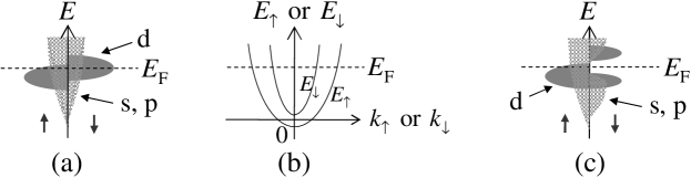
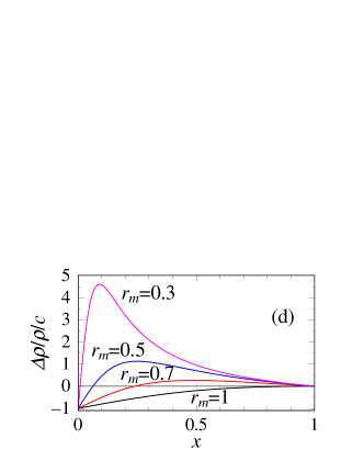
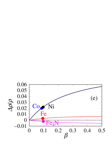
Figure 1: (Color online) (a) Partial DOSs of the s, p, and d states for the usual ferromagnets. (b) $E_{\sigma}$-$k_{\sigma}$ curve of the s and p states in (a). (c) Partial DOSs of the s, p, and d states for half-metallic Heusler alloys. In the case of the nearly HMF, there is a low DOS of the down spin at $E_{\mbox{\tiny F}}$. (d) $x$ dependence of $\Delta\rho/\rho/c$ of Eq. (5) with $x_{s}$=$x_{d}$$\equiv$$x$, $\beta_{\uparrow}$=$\beta_{\downarrow}$$\equiv$$\beta$, and $r_{m}$=0.3, 0.5, 0.7, and 1. (e) $\beta$ dependence of $\Delta\rho/\rho$ of Eq. (4) for Fe, Co, Ni, and Fe₄N is shown by solid curves. Here, we set $r_{m}$=1 and use parameters in Table 1. The black, blue, red, and purple dots show experimental results of $\Delta\rho/\rho$ at 300 K for Ni, Co, Fe, and Fe₄N, respectively (see Table 1).

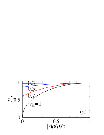
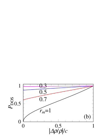
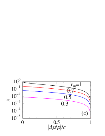
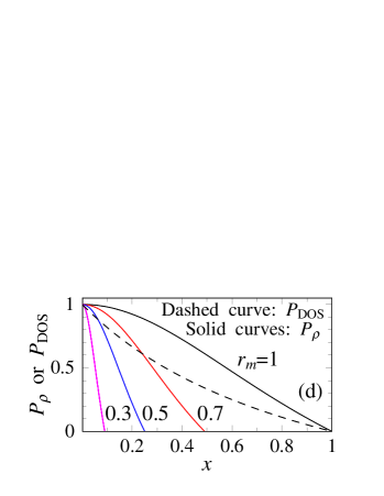
Figure 2: (Color online) (a) $|\Delta\rho/\rho|/c$ dependence of $P_{\rho}$ of Eq. (12). (b) $|\Delta\rho/\rho|/c$ dependence of $P_{\rm DOS}$ of Eq. ( Spin polarization ratios of resistivity and density of states estimated from anisotropic magnetoresistance ratio for nearly half-metallic ferromagnets ). (c) $|\Delta\rho/\rho|/c$ dependence of $x$ of Eq. (7). (d) $x$ dependences of $P_{\rho}$ of Eq. (11) and $P_{\rm DOS}$ of Eq. (8). Here, we set $r_{m}$=0.3, 0.5, 0.7, and 1, and $x_{s}$=$x_{d}$$\equiv$$x$.

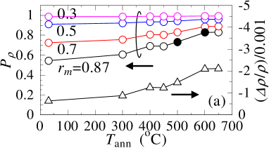
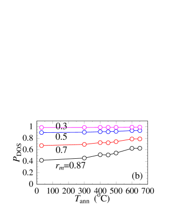
Figure 3: (Color online) (a) The white circles show the $T_{\rm ann}$ dependence of $P_{\rho}$ of Eq. (12) for CFGG, where $r_{m}$=0.3, 0.5, 0.7, and 0.87. The respective black dots denote the previously evaluated $P_{\rho}$ at $T_{\rm ann}$=500[12] and 600 ^∘C[13] in Table 2. The triangles show the experimental result of the $T_{\rm ann}$ dependence of $\Delta\rho/\rho$ at 300 K for CFGG.[6] (b) The $T_{\rm ann}$ dependence of $P_{\rm DOS}$ of Eq. ( Spin polarization ratios of resistivity and density of states estimated from anisotropic magnetoresistance ratio for nearly half-metallic ferromagnets ) for CFGG with $r_{m}$=0.3, 0.5, 0.7, and 0.87.

Table 1: Parameters $x_{s}$, $x_{d}$, and $y_{\uparrow}$, and experimental values of $\Delta\rho/\rho$ at 300 K for bcc Fe, fcc Co, fcc Ni, and Fe₄N. Each $x_{s}$ is evaluated from the values of $\rho_{s\downarrow}/\rho_{s\uparrow}$ and $\rho_{s\downarrow}/\rho_{s\uparrow}$=$r_{m}^{4}(D_{s\uparrow}/D_{s\downarrow})^{2}$ (Ref. Kokado1) with $r_{m}$=1.

Material	$x_{s}$	$x_{d}$ [8]	$y_{\uparrow}$	$\Delta\rho/\rho$ (experiment)
bcc Fe	1.6	0.50	25 (Ref. papa)	0.0030 (Ref. McGuire)
fcc Co	0.37	10	3.5 (Ref. comment)	0.020 (Ref. McGuire)
fcc Ni	0.32	10	3.5 (Ref. papa)	0.022 (Ref. McGuire)
Fe4N	25	5.0	20 (Ref. Sakuma)	$-$0.0021 (Ref. Tsunoda)

Table 2: Spin polarization ratios $P_{\rm DOS}$ of Eq. ( Spin polarization ratios of resistivity and density of states estimated from anisotropic magnetoresistance ratio for nearly half-metallic ferromagnets ) and $P_{\rho}$ of Eq. (12) at $T_{\rm ann}$=500 and 600 ^∘C for CFGG. They are the respective values at $r_{m}$=0.87 in Figs. 3(a) and 3(b). The previous values of $P_{\rho}$, which were evaluated on the basis of $\Delta RA$ at 300 K,[12, 13] are also noted.

$T_{\rm ann}$ (∘C)	$P_{\rm DOS}$ of Eq. ( Spin polarization ratios of resistivity and density of states estimated from anisotropic magnetoresistance ratio for nearly half-metallic ferromagnets )	$P_{\rho}$ of Eq. (12)	$P_{\rho}$ (previous values)
500	0.54	0.73	0.73$\pm$0.02 (Ref. Goripati)
600	0.62	0.83	0.83$\pm$0.02 (Ref. Li)

References

[1]
W. Thomson,
Proc. R. Soc. London 8, 546 (1856-1857).
[2]
T. R. McGuire, J. A. Aboaf, and E. Klokholm,
IEEE Trans. Magn. 20, 972 (1984).
[3]
T. Miyazaki and H. Jin,
The Physics of Ferromagnetism
(Springer, New York, 2012) Sect. 11.4.
[4]
M. Tsunoda, H. Takahashi, S. Kokado, Y. Komasaki, A. Sakuma, and M. Takahashi,
Appl. Phys. Express 3, 113003 (2010).
[5]
F. Yang, Y. Sakuraba, S. Kokado, Y. Kota, A. Sakuma, and K. Takanashi,
Phys. Rev. B 86, 020409 (2012).
[6]
Y. Sakuraba, S. Kokado, Y. Hirayama, T. Furubayashi, H. Sukegawa,
S. Li, Y. K. Takahashi, and K. Hono,
Appl. Phys. Lett. 104, 172407 (2014).
[7]
S. Li, Y. K. Takahashi, Y. Sakuraba, N. Tsuji, H. Tajiri,
Y. Miura, J. Chen, T. Furubayashi, and K. Hono,
Appl. Phys. Lett. 108, 122404 (2016).
[8]
S. Kokado, M. Tsunoda, K. Harigaya, and A. Sakuma,
J. Phys. Soc. Jpn. 81, 024705 (2012).
[9]
S. Kokado and M. Tsunoda,
Adv. Mater. Res. 750-752, 978 (2013).
[10]
S. Kokado and M. Tsunoda,
J. Phys. Soc. Jpn. 84, 094710 (2015).
[11]
T. Valet and A. Fert,
Phys. Rev. B 48, 7099 (1993).
[12]
H. S. Goripati, T. Furubayashi, Y. K. Takahashi, and K. Hono,
J. Appl. Phys. 113, 043901 (2013).
[13]
S. Li, Y. K. Takahashi, T. Furubayashi, and K. Hono,
Appl. Phys. Lett. 103, 042405 (2013).
[14]
B. S. D. C. S. Varaprasad, A. Srinivasan, Y. K. Takahashi,
M. Hayashi, A. Rajanikanth, and K. Hono,
Acta Mater. 60,6257 (2012).
[15]
The – scattering rate due to phonons
is proportional to
in the high temperature range including 300 K,
with being the temperature.
We here have .
As to the scattering rate due to phonons,
see
H. Nishimura, KisoKotaiDenshiRon (Basic Electron Theory of Solids)
(Gihodo Shuppan, Tokyo, 2003) p. 137 [in Japanese].
[16]
C. Kittel, Introduction to Solid State Physics
(Wiley, New York, 1986) 6th ed., p. 193.
[17]
As seen from Fig. 1(d),
systems with 1 and 0 can have ,
which corresponds to nearly HMFs.
In contrast, systems with 1 and 0
take a relatively large .
Only these systems should actually be called non-HMFs.
[18]
Note that
in Eq. (10)
[i.e., of Eq. (7)]
contains not but
with 01.
[19]
Note that
real HMFs may exhibit 1 at finite
because the down-spin electrons
are thermally excited from the valence band to the conduction band.
Therefore, in the HMF case of =0,
Eq. (11) is valid at 0 K and
appropriate for
and .
[20]
S. Sharma and S. K. Pandey,
J. Phys.: Condens. Matter 26, 215501 (2014).
[21]
D. A. Papaconstantopoulos,
Handbook of the Band Structure of Elemental Solids
(Plenum, New York, 1986) p. 95 and 111.
[22]
We utilize the same as that of the fcc Ni
because of the same crystal structure and
the small difference in the number of electrons.
[23]
A. Sakuma, J. Phys. Soc. Jpn. 60, 2007 (1991).
[24]
The CFGG with the 21 structure
has
0.5 eV and
0.2 eV,[14]
which
are much larger than =0.026 eV,
with =300 K.
[25]
In this study, we consider the case of 1
because with 1 tends to be very small.
Although with =1.15 agrees with the previous value at
=600 ∘C,
with =1.15 becomes 0.42,
which is less than (0.5) of Co.
This (=0.42) appears to be inappropriate for
the present CFGG,[6] which is regarded as the nearly HMF.
[26]
As a different method from the present one,
we note that
may be roughly evaluated from the above-mentioned equation,
=,
where
is obtained by, for example, first-principles calculation.