A first-order primal-dual algorithm with linesearch

Abstract

The paper proposes a linesearch for a primal-dual method. Each iteration of the linesearch requires to update only the dual (or primal) variable. For many problems, in particular for regularized least squares, the linesearch does not require any additional matrix-vector multiplications. We prove convergence of the proposed method under standard assumptions. We also show an ergodic $O(1/N)$ rate of convergence for our method. In case one or both of the prox-functions are strongly convex, we modify our basic method to get a better convergence rate. Finally, we propose a linesearch for a saddle point problem with an additional smooth term. Several numerical experiments confirm the efficiency of our proposed methods.

2010 Mathematics Subject Classification: 49M29 65K10 65Y20 90C25

Keywords: Saddle-point problems, first-order algorithms, primal-dual algorithms, linesearch, convergence rates, backtracking

In this work we propose a linesearch procedure for the primal-dual algorithm (PDA) that was introduced in [4]. It is a simple first-order method that is widely used for solving nonsmooth composite minimization problems. Recently, it was shown the connection of PDA with proximal point algorithms [12] and ADMM [6]. Some generalizations of the method were considered in [5, 10, 7]. A survey of possible applications of the algorithm can be found in [13, 6].

The basic form of PDA uses fixed step sizes during all iterations. This has several drawbacks. First, we have to compute the norm of the operator, which may be quite expensive for large scale dense matrices. Second, even if we know this norm, one can often use larger steps, which usually yields a faster convergence. As a remedy for the first issue one can use a diagonal precondition [16], but still there is no strong evidence that such a precondition improves or at least does not worsen the speed of convergence of PDA. Regarding the second issue, as we will see in our experiments, the speed improvement gained by using the linesearch sometimes can be significant.

Our proposed analysis of PDA exploits the idea of recent works [14, 15] where several algorithms are proposed for solving a monotone variational inequality. Those algorithms are different from the PDA; however, they also use a similar extrapolation step. Although our analysis of the primal-dual method is not so elegant as, for example, that in [12], it gives a simple and a cheap way to incorporate the linesearch for defining the step sizes. Each inner iteration of the linesearch requires updating only the dual variables. Moreover, the step sizes may increase from iteration to iteration. We prove the convergence of the algorithm under quite general assumptions. Also we show that in many important cases the PDAL (primal-dual algorithm with linesearch) preserves the complexity of the iteration of PDA. In particular, our method, applied to the regularized least-squares problems, uses the same number of matrix-vector multiplication per iteration as the forward-backward method or FISTA [3] (both with fixed step size) does, but does not require to know the matrix norm and, in addition, uses adaptive steps.

For the case when the primal or dual objectives are strongly convex, we modify our linesearch procedure in order to construct accelerated versions of PDA. This is done in a similar way as in [4]. The obtained algorithms share the same complexity per iteration as PDAL does, but in many cases substantially outperform PDA and PDAL.

We also consider a more general primal-dual problem which involves an additional smooth function with Lipschitz-continuous gradient (see [7]). For this case we generalize our linesearch to avoid knowing that Lipschitz constant.

The authors in [10, 9] also proposed a linesearch for the primal-dual method, with the goal to vary the ratio between primal and dual steps such that primal and dual residuals remain roughly of the same size. The same idea was used in [11] for the ADMM method. However, we should highlight that this principle is just a heuristic, as it is not clear that it in fact improves the speed of convergence. The linesearch proposed in [10, 9] requires an update of both primal and dual variables, which may make the algorithm much more expensive than the basic PDA. Also the authors proved convergence of the iterates only in the case when one of the sequences $(x^{k})$ or $(y^{k})$ is bounded. Although this is often the case, there are many problems which can not be encompassed by this assumption. Finally, it is not clear how to derive accelerated versions of that algorithm.

As a byproduct of our analysis, we show how one can use a variable ratio between primal and dual steps and under which circumstances we can guarantee convergence. However, it was not the purpose of this paper to develop new strategies for varying such a ratio during iterations.

The paper is organized as follows. In the next section we introduce the notations and recall some useful facts. Section 2 presents our basic primal-dual algorithm with linesearch. We prove its convergence, establish its ergodic convergence rate and consider some particular examples of how the linesearch works. In section 3 we propose accelerated versions of PDAL under the assumption that the primal or dual problem is strongly convex. Section 4 deals with more general saddle point problems which involve an additional smooth function. In section 5 we illustrate the efficiency of our methods for several typical problems.

1 Preliminaries

Let $X$, $Y$ be two finite-dimensional real vector spaces equipped with an inner product $\langle\cdot,\cdot\rangle$ and a norm $\|\cdot\|=\sqrt{\langle\cdot,\cdot\rangle}$. We are focusing on the following problem:

$$\min_{x\in X}\max_{y\in Y}\langle Kx,y\rangle+g(x)-f^{*}(y),$$ (1)

where

• $K\colon X\to Y$ is a bounded linear operator, with the operator norm $L=\|K\|$;

• $g\colon X\to(-\infty,+\infty]$ and $f^{*}\colon Y\to(-\infty,+\infty]$ are proper lower semicontinuous convex (l.s.c.) functions;

• problem (1) has a saddle point.

Note that $f^{*}$ denotes the Legendre–Fenchel conjugate of a convex l.s.c. function $f$. By a slight (but common) abuse of notation, we write $K^{*}$ to denote the adjoint of the operator $K$.

Under the above assumptions, (1) is equivalent to the primal problem

$$\min_{x\in X}f(Kx)+g(x)$$ (2)

and the dual problem:

$$\min_{y\in Y}f^{*}(y)+g^{*}(-K^{*}x).$$ (3)

Recall that for a proper l.s.c. convex function $h\colon X\to(-\infty,+\infty]$ the proximal operator $\operatorname{prox}_{h}$ is defined as

$$\operatorname{prox}_{h}\colon X\to X\colon x\mapsto\operatorname{argmin}_{z}\bigl{\{}h(z)+\frac{1}{2}\|z-x\|^{2}\bigr{\}}.$$

The following important characteristic property of the proximal operator is well known:

$$\bar{x}=\operatorname{prox}_{h}x\quad\Leftrightarrow\quad\langle\bar{x}-x,y-\bar{x}\rangle\geq h(\bar{x})-h(y)\quad\forall y\in X.$$ (4)

We will often use the following identity (cosine rule):

$$2\langle a-b,c-a\rangle=\|b-c\|^{2}-\|a-b\|^{2}-\|a-c\|^{2}\quad\forall a,b,c\in X.$$ (5)

Let $(\hat{x},\hat{y})$ be a saddle point of problem (1). Then by the definition of the saddle point we have

$$P_{\hat{x},\hat{y}}(x):=g(x)-g(\hat{x})+\langle K^{*}\hat{y},x-\hat{x}\rangle\geq 0\quad\forall x\in X,$$ (6)

$$D_{\hat{x},\hat{y}}(y):=f^{*}(y)-f^{*}(\hat{y})-\langle K\hat{x},y-\hat{y}\rangle\geq 0\quad\forall y\in Y.$$ (7)

The expression $\mathcal{G}_{\hat{x},\hat{y}}(x,y)=P_{\hat{x},\hat{y}}(x)+D_{\hat{x},\hat{y}}(y)$ is known as a primal-dual gap. In certain cases when it is clear which saddle point is considered, we will omit the subscript in $P$, $D$, and $\mathcal{G}$. It is also important to highlight that for fixed $(\hat{x},\hat{y})$ functions $P(\cdot)$, $D(\cdot)$, and $\mathcal{G}(\cdot,\cdot)$ are convex.

Consider the original primal-dual method:

$$y^{k+1} =\operatorname{prox}_{\sigma f^{*}}(y^{k}+\sigma K\bar{x}^{k})$$

$$x^{k+1} =\operatorname{prox}_{\tau g}(x^{k}-\tau K^{*}y^{k+1})$$

$$\bar{x}^{k+1} =x^{k+1}+\theta(x^{k+1}-x^{k}).$$

In [4] its convergence was proved under assumptions $\theta=1$, $\tau,\sigma>0$, and $\tau\sigma L^{2}<1$. In the next section we will show how to incorporate a linesearch into this method.

2 Linesearch

The primal-dual algorithm with linesearch (PDAL) is summarized in Algorithm 1.

Algorithm 1 Primal-dual algorithm with linesearch

  Initialization: Choose $x^{0}\in X$, $y^{1}\in Y$, $\tau_{0}>0$, $\mu\in(0,1),\delta\in(0,1)$, and $\beta>0$. Set $\theta_{0}=1$.

  Main iteration:

  1. Compute

$$x^{k}=\operatorname{prox}_{\tau_{k-1}g}(x^{k-1}-\tau_{k-1}K^{*}y^{k}).$$

  2. Choose any $\tau_{k}\in[\tau_{k-1},\tau_{k-1}\sqrt{1+\theta_{k-1}}]$ and run

      Linesearch:

      2.a. Compute

$$\theta_{k} =\frac{\tau_{k}}{\tau_{k-1}}$$

$$\bar{x}^{k} =x^{k}+\theta_{k}(x^{k}-x^{k-1})$$

$$y^{k+1} =\operatorname{prox}_{\beta\tau_{k}f^{*}}(y^{k}+\beta\tau_{k}K\bar{x}^{k})$$

     2.b. Break linesearch if

$$\sqrt{\beta}\tau_{k}\|K^{*}y^{k+1}-K^{*}y^{k}\|\leq\delta\|y^{k+1}-y^{k}\|$$ (8)

         Otherwise, set $\tau_{k}:=\tau_{k}\mu$ and go to 2.a.

     End of linesearch

Given all information from the current iterate: $x^{k}$, $y^{k}$, $\tau_{k-1}$, and $\theta_{k-1}$, we first choose some trial step $\tau_{k}\in[\tau_{k-1},\tau_{k-1}\sqrt{1+\theta_{k-1}}]$, then during every iteration of the linesearch it is decreased by $\mu\in(0,1)$. At the end of the linesearch we obtain a new iterate $y^{k+1}$ and a step size $\tau_{k}$ which will be used to compute the next iterate $x^{k+1}$. In Algorithm 1 there are two opposite options: always start the linesearch from the largest possible step $\tau_{k}=\tau_{k-1}\sqrt{1+\theta_{k-1}}$, or, the contrary, never increase $\tau_{k}$. Step 2 also allows us to choose compromise between them.

Note that in PDAL parameter $\beta$ plays the role of the ratio $\frac{\sigma}{\tau}$ between fixed steps in PDA. Thus, we can rewrite the stopping criteria (8) as

$$\tau_{k}\sigma_{k}\|K^{*}y^{k+1}-K^{*}y^{k}\|^{2}\leq\delta^{2}\|y^{k+1}-y^{k}\|^{2},$$

where $\sigma_{k}=\beta\tau_{k}$. Of course in PDAL we can always choose fixed steps $\tau_{k}$, $\sigma_{k}$ with $\tau_{k}\sigma_{k}\leq\frac{\delta^{2}}{L^{2}}$ and set $\theta_{k}=1$. In this case PDAL will coincide with PDA, though our proposed analysis seems to be new. Parameter $\delta$ is mainly used for theoretical purposes: in order to be able to control $\|y^{k+1}-y^{k}\|^{2}$, we need $\delta<1$. For the experiments $\delta$ should be chosen very close to $1$.

Remark 1.

It is clear that each iteration of the linesearch requires computation of $\operatorname{prox}_{\beta\tau_{k}f^{*}}(\cdot)$ and $K^{*}y^{k+1}$. As in problem (1) we can always exchange primal and dual variables, hence it makes sense to choose for the dual variable in PDAL the one for which the respective prox-operator is simpler to compute. Note that during the linesearch we need to compute $Kx^{k}$ only once and then use that $K\bar{x}^{k}=(1+\theta_{k})Kx^{k}-\theta_{k}Kx^{k-1}$.

Remark 2.

Note that when $\operatorname{prox}_{\sigma f^{*}}$ is a linear (or affine) operator, the linesearch becomes extremely simple: it does not require any additional matrix-vector multiplications. We itemize some examples below:

1. $f^{*}(y)=\langle c,y\rangle$. Then it is easy to verify that $\operatorname{prox}_{\sigma f^{*}}u=u-\sigma c$. Thus, we have

   $$y^{k+1} =\operatorname{prox}_{\sigma_{k}f^{*}}(y^{k}+\sigma_{k}K\bar{x}^{k})=y^{k}+\sigma_{k}K\bar{x}^{k}-\sigma_{k}c$$

   $$K^{*}y^{k+1} =K^{*}y^{k}+\sigma_{k}(K^{*}K\bar{x}^{k}-K^{*}c)$$

2. $f^{*}(y)=\frac{1}{2}\|y-b\|^{2}$. Then $\operatorname{prox}_{\sigma f^{*}}u=\frac{u+\sigma b}{1+\sigma}$ and we obtain

   $$y^{k+1} =\operatorname{prox}_{\sigma_{k}f^{*}}(y^{k}+\sigma_{k}K\bar{x}^{k})=\frac{y^{k}+\sigma_{k}(K\bar{x}^{k}+b)}{1+\sigma_{k}}$$

   $$K^{*}y^{k+1} =\frac{1}{1+\sigma_{k}}(K^{*}y^{k}+\sigma_{k}(K^{*}K\bar{x}^{k}+K^{*}b))$$

3. $f^{*}(y)=\delta_{H}(y)$, the indicator function of the hyperplane $H=\{u\colon\langle u,a\rangle=b\}$. Then $\operatorname{prox}_{\sigma f^{*}}u=P_{H}u=u+\frac{b-\langle u,a\rangle}{\|a\|^{2}}a$. And hence,

   $$y^{k+1} =\operatorname{prox}_{\sigma_{k}f^{*}}(y^{k}+\sigma_{k}K\bar{x}^{k})=y^{k}+\sigma_{k}K\bar{x}^{k}+\frac{b-\langle a,y^{k}+\sigma_{k}K\bar{x}^{k}\rangle}{\|a\|^{2}}a$$

   $$K^{*}y^{k+1} =K^{*}y^{k}+\sigma_{k}K^{*}K\bar{x}^{k}+\frac{b-\langle a,y^{k}+\sigma_{k}K\bar{x}^{k}\rangle}{\|a\|^{2}}K^{*}a.$$

Evidently, each iteration of PDAL for all the cases above requires only two matrix-vector multiplications. Indeed, before the linesearch starts we have to compute $Kx^{k}$ and $K^{*}Kx^{k}$ and then during the linesearch we should use the following relations:

$$K\bar{x}^{k} =(1+\theta_{k})Kx^{k}-\theta_{k}Kx^{k-1}$$

$$K^{*}K\bar{x}^{k} =(1+\theta_{k})K^{*}Kx^{k}-\theta_{k}K^{*}Kx^{k-1},$$

where $Kx^{k-1}$ and $K^{*}Kx^{k-1}$ should be reused from the previous iteration. All other operations are comparably cheap and, hence, the cost per iteration of PDA and PDAL are almost the same. However, this might not be true if the matrix $K$ is very sparse. For example, for a finite differences operator the cost of a matrix-vector multiplication is the same as the cost of a few vector-vector additions.

One simple implication of these facts is that for the regularized least-squares problem

$$\min_{x}\frac{1}{2}\|Ax-b\|^{2}+g(x),$$ (9)

our method does not require one to know $\|A\|$ but at the same time does not require any additional matrix-vector multiplication as it is the case for standard first order methods with backtracking (e.g. proximal gradient method, FISTA). In fact, we can rewrite (9) as

$$\min_{x}\max_{y}g(x)+\langle Ax,y\rangle-\frac{1}{2}\|y+b\|^{2}.$$ (10)

Here $f^{*}(y)=\frac{1}{2}\|y+b\|^{2}$ and hence, we are in the situation where the operator $\operatorname{prox}_{f^{*}}$ is affine.

By construction of the algorithm we simply have the following:

Lemma 1.

(i)

The linesearch in PDAL always terminates.

(ii)

There exists $\tau>0$ such that $\tau_{k}>\tau$ for all $k\geq 0$.

(iii)

There exists $\theta>0$ such that $\theta_{k}\leq\theta$ for all $k\geq 0$.

Proof.

(i) In each iteration of the linesearch $\tau_{k}$ is multiplied by factor $\mu<1$. Since, (8) is satisfied for any $\tau_{k}\leq\frac{\delta}{\sqrt{\beta}L}$, the inner loop can not run indefinitely.

(ii) Without loss of generality, assume that $\tau_{0}>\frac{\delta\mu}{\sqrt{\beta}L}$. Our goal is to show that from $\tau_{k-1}>\frac{\delta\mu}{\sqrt{\beta}L}$ follows $\tau_{k}>\frac{\delta\mu}{\sqrt{\beta}L}$. Suppose that $\tau_{k}=\tau_{k-1}\sqrt{1+\theta_{k-1}}\mu^{i}$ for some $i\in\mathbb{Z}^{+}$. If $i=0$ then $\tau_{k}>\tau_{k-1}>\frac{\delta\mu}{\sqrt{\beta}L}$. If $i>0$ then $\tau_{k}^{\prime}=\tau_{k-1}\sqrt{1+\theta_{k-1}}\mu^{i-1}$ does not satisfy (8). Thus, $\tau_{k}^{\prime}>\frac{\delta}{\sqrt{\beta}L}$ and hence, $\tau_{k}>\frac{\delta\mu}{\sqrt{\beta}L}$.

(iii) From $\tau_{k}\leq\tau_{k-1}\sqrt{1+\theta_{k-1}}$ and $\theta_{k}=\frac{\tau_{k}}{\tau_{k-1}}$ it follows that $\theta_{k}\leq\sqrt{1+\theta_{k-1}}$. From this it can be easily concluded that $\theta_{k}\leq\frac{\sqrt{5}+1}{2}$ for all $k\in\mathbb{Z}^{+}$. In fact, assume the contrary, and let $r$ be the smallest number such that $\theta_{r}>\frac{\sqrt{5}+1}{2}$. Since $\theta_{0}=1$, we have $r\geq 1$, and hence $\theta_{r-1}\geq\theta_{r}^{2}-1>\frac{\sqrt{5}+1}{2}$. This yields a contradiction. ∎

One might be interested in how many iterations the linesearch needs in order to terminate. Of course, we can give only a priori upper bounds. Assume that $(\tau_{k})$ is bounded from above by $\tau_{max}$. Consider in step 2 of Algorithm 1 two opposite ways of choosing step size $\tau_{k}$: maximally increase it, that is, always set $\tau_{k}=\tau_{k-1}\sqrt{1+\theta_{k-1}}$ or never increase it and set $\tau_{k}=\tau_{k-1}$. If the former case holds, then after $i$ iterations of the linesearch we have $\tau_{k}\leq\tau_{k-1}\sqrt{1+\theta_{k-1}}\mu^{i-1}\leq\tau_{max}\frac{\sqrt{5}+1}{2}\mu^{i-1}$, where we have used the bound from Lemma 1 (iii). Hence, if $i-1\geq\log_{\mu}\frac{2\delta}{\beta L(1+\sqrt{5})\tau_{max}}$, then $\tau_{k}\leq\frac{\delta}{\beta L}$ and the linesearch procedure must terminate. Similarly, if the latter case holds, then after at most $1+\log_{\mu}\frac{\delta}{\beta L\tau_{max}}$ iterations the linesearch stops. However, because in this case $(\tau_{k})$ is nonincreasing, this number is the upper bound for the total number of the linesearch iterations.

The following is our main convergence result.

Theorem 1.

Let $(x^{k},y^{k})$ be a sequence generated by PDAL. Then it is a bounded sequence in $X\times Y$ and all its cluster points are solutions of (1). Moreover, if $g|_{\operatorname{dom}g}$ is continuous and $(\tau_{k})$ is bounded from above then the whole sequence $(x^{k},y^{k})$ converges to a solution of (1).

The condition of $g|_{\operatorname{dom}g}$ to be continuous is not restrictive: it holds for any $g$ with open $\operatorname{dom}g$ (this includes all finite-valued functions) or for an indicator $\delta_{C}$ of any closed convex set $C$. Also it holds for any separable convex l.s.c. function (Corollary 9.15, [2]). The boundedness of $(\tau_{k})$ from above is rather theoretical: clearly we can easily bound it in PDAL.

Proof.

Let $(\hat{x},\hat{y})$ be any saddle point of (1). From (4) it follows that

$$\langle x^{k+1}-x^{k}+\tau_{k}K^{*}y^{k+1},\hat{x}-x^{k+1}\rangle\geq\tau_{k}(g(x^{k+1})-g(\hat{x}))$$ (11)

$$\bigl{\langle}\frac{1}{\beta}(y^{k+1}-y^{k})-\tau_{k}K\bar{x}^{k},\hat{y}-y^{k+1}\bigr{\rangle}\geq\tau_{k}(f^{*}(y^{k+1})-f^{*}(\hat{y})).$$ (12)

Since $x^{k}=\operatorname{prox}_{\tau_{k-1}g}(x^{k-1}-\tau_{k-1}K^{*}y^{k})$, we have again by (4) that for all $x\in X$

$$\langle x^{k}-x^{k-1}+\tau_{k-1}K^{*}y^{k},x-x^{k}\rangle\geq\tau_{k-1}(g(x^{k})-g(x)).$$

After substitution in the last inequality $x=x^{k+1}$ and $x=x^{k-1}$ we get

$$\langle x^{k}-x^{k-1}+\tau_{k-1}K^{*}y^{k},x^{k+1}-x^{k}\rangle\geq\tau_{k-1}(g(x^{k})-g(x^{k+1})),$$ (13)

$$\langle x^{k}-x^{k-1}+\tau_{k-1}K^{*}y^{k},x^{k-1}-x^{k}\rangle\geq\tau_{k-1}(g(x^{k})-g(x^{k-1})).$$ (14)

Adding (13), multiplied by $\theta_{k}=\frac{\tau_{k}}{\tau_{k-1}}$, and (14), multiplied by $\theta_{k}^{2}$, we obtain

$$\langle\bar{x}^{k}-x^{k}+\tau_{k}K^{*}y^{k},x^{k+1}-\bar{x}^{k}\rangle\geq\tau_{k}((1+\theta_{k})g(x^{k})-g(x^{k+1})-\theta_{k}g(x^{k-1})),$$ (15)

where we have used that $\bar{x}^{k}=x^{k}+\theta_{k}(x^{k}-x^{k-1})$.

Consider the following identity:

$$\tau_{k}\langle K^{*}y^{k+1}-K^{*}\hat{y},\bar{x}^{k}-\hat{x}\rangle-\tau_{k}\langle K\bar{x}^{k}-K\hat{x},y^{k+1}-\hat{y}\rangle=0.$$ (16)

Summing (11), (12), (15), and (16), we get

$$\langle x^{k+1}-x^{k},\hat{x}-x^{k+1}\rangle+\frac{1}{\beta}\langle y^{k+1}-y^{k},\hat{y}-y^{k+1}\rangle+\langle\bar{x}^{k}-x^{k},x^{k+1}-\bar{x}^{k}\rangle\\ +\tau_{k}\langle K^{*}y^{k+1}-K^{*}y^{k},\bar{x}^{k}-x^{k+1}\rangle-\tau_{k}\langle K^{*}y,\bar{x}^{k}-\hat{x}\rangle+\tau_{k}\langle K\hat{x},y^{k+1}-y\rangle\\ \geq\tau_{k}\bigl{(}f^{*}(y^{k+1})-f^{*}(\hat{y})+(1+\theta_{k})g(x^{k})-\theta_{k}g(x^{k-1})-g(\hat{x})\bigr{)}.$$ (17)

Using that

$$f^{*}(y^{k+1})-f^{*}(\hat{y})-\langle K\hat{x},y^{k+1}-\hat{y}\rangle=D_{\hat{x},\hat{y}}(y^{k+1})$$ (18)

and

$$(1+ \theta_{k})g(x^{k})-\theta_{k}g(x^{k-1})-g(\hat{x})+\langle K^{*}y,\bar{x}^{k}-\hat{x}\rangle$$

$$=(1+\theta_{k})\left(g(x^{k})-g(\hat{x})+\langle K^{*}\hat{y},x^{k}-\hat{x}\rangle\right)-\theta_{k}\left(g(x^{k-1})-g(\hat{x})+\langle K^{*}\hat{y},x^{k-1}-\hat{x}\rangle\right)$$

$$=(1+\theta_{k})P_{\hat{x},\hat{y}}(x^{k})-\theta_{k}P_{\hat{x},\hat{y}}(x^{k-1}),$$ (19)

we can rewrite (17) as (we will not henceforth write the subscripts for $P$ and $D$ unless it is unclear)

$$\langle x^{k+1}-x^{k},\hat{x}-x^{k+1}\rangle+\frac{1}{\beta}\langle y^{k+1}-y^{k},\hat{y}-y^{k+1}\rangle+\langle\bar{x}^{k}-x^{k},x^{k+1}-\bar{x}^{k}\rangle\\ +\tau_{k}\langle K^{*}y^{k+1}-K^{*}y^{k},\bar{x}^{k}-x^{k+1}\rangle\geq\tau_{k}((1+\theta_{k})P(x^{k})-\theta_{k}P(x^{k-1})+D(y^{k+1})).$$ (20)

Let $\varepsilon_{k}$ denotes the right-hand side of (20). Using the cosine rule for every item in the first line of (20), we obtain

$$\frac{1}{2}(\|x^{k}-\hat{x}\|^{2}-\|x^{k+1}-\hat{x}\|^{2}-\|x^{k+1}-x^{k}\|^{2})\\ +\frac{1}{2\beta}(\|y^{k}-\hat{y}\|^{2}-\|y^{k+1}-\hat{y}\|^{2}-\|y^{k+1}-y^{k}\|^{2})\\ +\frac{1}{2}(\|x^{k+1}-x^{k}\|^{2}-\|\bar{x}^{k}-x^{k}\|^{2}-\|x^{k+1}-\bar{x}^{k}\|^{2})\\ +\tau_{k}\langle K^{*}y^{k+1}-K^{*}y^{k},\bar{x}^{k}-x^{k+1}\rangle\geq\varepsilon_{k}.$$ (21)

By (8), Cauchy–Schwarz, and Cauchy’s inequalities we get

$$\tau_{k}\langle K^{*}y^{k+1}-K^{*}y^{k},\bar{x}^{k}-x^{k+1}\rangle \leq\frac{\delta}{\sqrt{\beta}}\|x^{k+1}-\bar{x}^{k}\|\|y^{k+1}-y^{k}\|$$

$$\leq\frac{1}{2}\|x^{k+1}-\bar{x}^{k}\|^{2}+\frac{\delta^{2}}{2\beta}\|y^{k+1}-y^{k}\|^{2},$$

from which we derive that

$$\frac{1}{2}(\|x^{k}-\hat{x}\|^{2}-\|x^{k+1}-\hat{x}\|^{2})+\frac{1}{2\beta}(\|y^{k}-\hat{y}\|^{2}-\|y^{k+1}-\hat{y}\|^{2})\\ -\frac{1}{2}\|\bar{x}^{k}-x^{k}\|^{2}-\frac{1-\delta^{2}}{2\beta}\|y^{k+1}-y^{k}\|^{2}\geq\varepsilon_{k}.$$ (22)

Since $(\hat{x},\hat{y})$ is a saddle point, $D(y^{k})\geq 0$ and $P(x^{k})\geq 0$ and hence (22) yields

$$\frac{1}{2}(\|x^{k}-\hat{x}\|^{2}-\|x^{k+1}-\hat{x}\|^{2})+\frac{1}{2\beta}(\|y^{k}-\hat{y}\|^{2}-\|y^{k+1}-\hat{y}\|^{2})\\ -\frac{1}{2}\|\bar{x}^{k}-x^{k}\|^{2}-\frac{1-\delta^{2}}{2\beta}\|y^{k+1}-y^{k}\|^{2}\geq\tau_{k}((1+\theta_{k})P(x^{k})-\theta_{k}P(x^{k-1}))$$ (23)

or, taking into account $\theta_{k}\tau_{k}\leq(1+\theta_{k-1})\tau_{k-1}$,

$$\frac{1}{2}\|x^{k+1}-\hat{x}\|^{2}+\frac{1}{2\beta}\|y^{k+1}-\hat{y}\|^{2}+\tau_{k}(1+\theta_{k})P(x^{k})\leq\\ \frac{1}{2}\|x^{k}-\hat{x}\|^{2}+\frac{1}{2\beta}\|y^{k}-\hat{y}\|^{2}+\tau_{k-1}(1+\theta_{k-1})P(x^{k-1})\\ -\frac{1}{2}\|\bar{x}^{k}-x^{k}\|^{2}-\frac{1-\delta^{2}}{2\beta}\|y^{k+1}-y^{k}\|^{2}$$ (24)

From this we deduce that $(x^{k})$, $(y^{k})$ are bounded sequences and $\lim_{k\to\infty}\|\bar{x}^{k}-x^{k}\|=0$, $\lim_{k\to\infty}\|y^{k}-y^{k-1}\|=0$. Also notice that

$$\frac{x^{k+1}-x^{k}}{\tau_{k}}=\frac{\bar{x}^{k+1}-x^{k+1}}{\tau_{k+1}}\to 0\quad\text{as }k\to\infty,$$

where the latter holds because $\tau_{k}$ is separated from $0$ by Lemma 1. Let $(x^{k_{i}},y^{k_{i}})$ be a subsequence that converges to some cluster point $(x^{*},y^{*})$. Passing to the limit in

$$\langle\frac{1}{\tau_{k_{i}}}(x^{k_{i}+1}-x^{k_{i}})+K^{*}y^{k_{i}},x-x^{k_{i}+1}\rangle \geq g(x^{k_{i}+1})-g(x)\quad\forall x\in X,$$

$$\langle\frac{1}{\beta\tau_{k_{i}}}(y^{k_{i}+1}-y^{k_{i}})-K\bar{x}^{k_{i}},y-y^{k_{i}+1}\rangle \geq f^{*}(y^{k_{i}+1})-f^{*}(y)\quad\forall y\in Y,$$

we obtain that $(x^{*},y^{*})$ is a saddle point of (1).

When $g|_{\operatorname{dom}g}$ is continuous, $g(x^{k_{i}})\to g(x^{*})$, and hence, $P_{x^{*},y^{*}}(x^{k_{i}})\to 0$. From (24) it follows that the sequence $a_{k}=\frac{1}{2}\|x^{k+1}-x^{*}\|^{2}+\frac{1}{2\beta}\|y^{k+1}-y^{*}\|^{2}+\tau_{k}(1+\theta_{k})P_{x^{*},y^{*}}(x^{k})$ is monotone. Taking into account boundedness of $(\tau_{k})$ and $(\theta_{k})$, we obtain

$$\lim_{k\to\infty}a_{k}=\lim_{i\to\infty}a_{k_{i}}=0,$$

which means that $x^{k}\to x^{*}$, $y^{k}\to y^{*}$. ∎

Theorem 2 (ergodic convergence).

Let $(x^{k},y^{k})$ be a sequence generated by PDAL and $(\hat{x},\hat{y})$ be any saddle point of (1). Then for the ergodic sequence $(X^{N},Y^{N})$ it holds that

$$\mathcal{G}_{\hat{x},\hat{y}}(X^{N},Y^{N})\leq\frac{1}{s_{N}}\left(\frac{1}{2}\|x^{1}-\hat{x}\|^{2}+\frac{1}{2\beta}\|y^{1}-\hat{y}\|^{2}+\tau_{1}\theta_{1}P_{\hat{x},\hat{y}}(x^{0})\right),$$

where $s_{N}=\sum_{k=1}^{N}\tau_{k}$, $X^{N}=\dfrac{\tau_{1}\theta_{1}x^{0}+\sum_{k=1}^{N}\tau_{k}\bar{x}^{k}}{\tau_{1}\theta_{1}+s_{N}}$, $Y^{N}=\dfrac{\sum_{k=1}^{N}\tau_{k}y^{k}}{s_{N}}$.

Proof.

Summing up (22) from $k=1$ to $N$, we get

$$\frac{1}{2}(\|x^{1}-\hat{x}\|^{2}-\|x^{N+1}-\hat{x}\|^{2})+\frac{1}{2\beta}(\|y^{1}-\hat{y}\|^{2}-\|y^{N+1}-\hat{y}\|^{2})\geq\sum_{k=1}^{N}\varepsilon_{k}$$ (25)

The right-hand side in (25) can be expressed as

$$\sum_{k=1}^{N}\varepsilon_{k}=\tau_{N}(1+\theta_{N})P(x^{N}) +\sum_{k=2}^{N}[(1+\theta_{k-1})\tau_{k-1}-\theta_{k}\tau_{k})]P(x^{k-1})$$

$$-\theta_{1}\tau_{1}P(x^{0})+\sum_{k=1}^{N}\tau_{k}D(y^{k+1})$$

By convexity of $P$,

$$\tau_{N}(1+\theta_{N})P(x^{N})+ \sum_{k=2}^{N}[(1+\theta_{k-1})\tau_{k-1}-\theta_{k}\tau_{k})]P(x^{k-1})$$ (26)

$$\geq(\tau_{1}\theta_{1}+s_{N})P(\frac{\tau_{1}(1+\theta_{1})x^{1}+\sum_{k=2}^{N}\tau_{k}\bar{x}^{k}}{\tau_{1}\theta_{1}+s_{N}})$$ (27)

$$=(\tau_{1}\theta_{1}+s_{N})P(\frac{\tau_{1}\theta_{1}x^{0}+\sum_{k=1}^{N}\tau_{k}\bar{x}^{k}}{\tau_{1}\theta_{1}+s_{N}})\geq s_{N}P(X^{N}),$$ (28)

where $s_{N}=\sum_{k=1}^{N}\tau_{k}$. Similarly,

$$\sum_{k=1}^{N}\tau_{k}D(y^{k})\geq s_{N}D(\frac{\sum_{k=1}^{N}\tau_{k}y^{k}}{s_{N}})=s_{N}D(Y^{N}).$$ (29)

Hence,

$$\sum_{k=1}^{N}\varepsilon_{k}\geq s_{N}(P(X^{N})+D(Y^{N}))-\tau_{1}\theta_{1}P(x^{0})$$

and we conclude

$$\mathcal{G}(X^{N},Y^{N})=P(X^{N})+D(Y^{N})\leq\frac{1}{s_{N}}\left(\frac{1}{2}\|x^{1}-\hat{x}\|^{2}+\frac{1}{2\beta}\|y^{1}-\hat{y}\|^{2}+\tau_{1}\theta_{1}P(x^{0})\right).\qed$$

Clearly, we have the same $O(1/N)$ rate of convergence as in [4, 5, 9], though with the ergodic sequence $(X^{N},Y^{N})$ defined in a different way.

Analysing the proof of Theorems 1 and 2, the reader may find out that our proof does not rely on the proximal interpretation of the PDA [12]. An obvious shortcoming of our approach is that deriving new extensions of the proposed method, like inertial or relaxed versions [5], still requires some nontrivial efforts. It would be interesting to obtain a general approach for the proposed method and its possible extensions.

It is well known that in many cases the speed of convergence of PDA crucially depends on the ratio between primal and dual steps $\beta=\dfrac{\sigma}{\tau}$. Motivated by this, paper [10] proposed an adaptive strategy for how to choose $\beta$ in every iteration. Although it is not the goal of this work to study the strategies for defining $\beta$, we show that the analysis of PDAL allows us to incorporate such strategies in a very natural way.

Theorem 3.

Let $(\beta_{k})\subset(\beta_{min},\beta_{max})$ be a monotone sequence with $\beta_{min},\beta_{max}>0$ and $(x^{k},y^{k})$ be a sequence generated by PDAL with variable $(\beta_{k})$. Then the statement of Theorem 1 holds.

Proof.

Let $(\beta_{k})$ be nondecreasing. Then using $\frac{1}{\beta_{k}}\leq\frac{1}{\beta_{k-1}}$, we get from (24) that

$$\frac{1}{2}\|x^{k+1}-\hat{x}\|^{2}+\frac{1}{2\beta_{k}}\|y^{k+1}-\hat{y}\|^{2}+\tau_{k}(1+\theta_{k})P(x^{k})\leq\\ \frac{1}{2}\|x^{k}-\hat{x}\|^{2}+\frac{1}{2\beta_{k-1}}\|y^{k}-\hat{y}\|^{2}+\tau_{k-1}(1+\theta_{k-1})P(x^{k-1})\\ -\frac{1}{2}\|\bar{x}^{k}-x^{k}\|^{2}-\frac{1-\delta^{2}}{2\beta_{k}}\|y^{k+1}-y^{k}\|^{2}.$$ (30)

Since $(\beta_{k})$ is bounded from above, the conclusion in Theorem 1 simply follows.

If $(\beta_{k})$ is decreasing, then the above arguments should be modified. Consider (23), multiplied by $\beta_{k}$,

$$\frac{\beta_{k}}{2}(\|x^{k}-\hat{x}\|^{2}-\|x^{k+1}-\hat{x}\|^{2})+\frac{1}{2}(\|y^{k}-\hat{y}\|^{2}-\|y^{k+1}-\hat{y}\|^{2})\\ -\frac{\beta_{k}}{2}\|\bar{x}^{k}-x^{k}\|^{2}-\frac{1-\delta^{2}}{2}\|y^{k+1}-y^{k}\|^{2}\geq\beta_{k}\tau_{k}((1+\theta_{k})P(x^{k})-\theta_{k}P(x^{k-1})).$$ (31)

As $\beta_{k}<\beta_{k-1}$, we have $\theta_{k}\beta_{k}\tau_{k}\leq(1+\theta_{k-1})\beta_{k-1}\tau_{k-1}$, which in turn implies

$$\frac{\beta_{k}}{2}\|x^{k+1}-\hat{x}\|^{2}+\frac{1}{2}\|y^{k+1}-\hat{y}\|^{2}+\tau_{k}\beta_{k}(1+\theta_{k})P(x^{k})\leq\\ \frac{\beta_{k-1}}{2}\|x^{k}-\hat{x}\|^{2}+\frac{1}{2}\|y^{k}-\hat{y}\|^{2}+\tau_{k-1}\beta_{k-1}(1+\theta_{k-1})P(x^{k-1})\\ -\frac{\beta_{k}}{2}\|\bar{x}^{k}-x^{k}\|^{2}-\frac{1-\delta^{2}}{2}\|y^{k+1}-y^{k}\|^{2}.$$ (32)

Due to the given properties of $(\beta_{k})$, the rest is trivial. ∎

It is natural to ask if it is possible to use nonmonotone $(\beta_{k})$. To answer this question, we can easily use the strategies from [11], where an ADMM with variable steps was proposed. One way is to use any $\beta_{k}$ during a finite number of iterations and then switch to monotone $(\beta_{k})$. Another way is to relax the monotonicity of $(\beta_{k})$ to the following:

$$\text{there exists }(\rho_{k})\subset\mathbb{R}_{+}\quad\text{such that}\colon\sum_{k}\rho_{k} <\infty\quad\text{and}$$

$$\beta_{k} \leq\beta_{k-1}(1+\rho_{k})\quad\forall k\in\mathbb{N}\quad\text{or }$$

$$\beta_{k-1} \leq\beta_{k}(1+\rho_{k})\quad\forall k\in\mathbb{N}.$$

We believe that it should be quite straightforward to prove convergence of PDAL with the latter strategy.

3 Acceleration

It has been shown [4] that in the case when $g$ or $f^{*}$ is strongly convex, one can modify the primal-dual algorithm and derive a better convergence rate. We show that the same holds for PDAL. The main difference of the accelerated variant APDAL from the basic PDAL is that now we have to vary $\beta$ in every iteration.

Of course due to the symmetry of the primal and dual variables in (1), we can always assume that the primal objective is strongly convex. However, from the computational point of view it might not be desirable to exchange $g$ and $f^{*}$ in the PDAL because of Remark 2. Therefore, we discuss the two cases separately. Also notice that both accelerated algorithms below coincide with PDAL when the parameter of strong convexity $\gamma=0$.

3.1 $g$ is strongly convex

Assume that $g$ is $\gamma$–strongly convex, i.e.,

$$g(x_{2})-g(x_{1})\geq\langle u,x_{2}-x_{1}\rangle+\frac{\gamma}{2}\|x_{2}-x_{1}\|^{2}\quad\forall x_{1},x_{2}\in X,u\in\partial g(x_{1}).$$

Below we assume that the parameter $\gamma$ is known. The following algorithm (APDAL) exploits the strong convexity of $g$:

Algorithm 2 Accelerated primal-dual algorithm with linesearch: $g$ is strongly convex

  Initialization: Choose $x^{0}\in X$, $y^{1}\in Y$, $\mu\in(0,1)$, $\tau_{0}>0$, $\beta_{0}>0$. Set $\theta_{0}=1$.

  Main iteration:

  1. Compute

$$x^{k} =\operatorname{prox}_{\tau_{k-1}g}(x^{k-1}-\tau_{k-1}K^{*}y^{k})$$

$$\beta_{k} =\beta_{k-1}(1+\gamma\tau_{k-1})$$

  2. Choose any $\tau_{k}\in[\tau_{k-1}\sqrt{\frac{\beta_{k-1}}{\beta_{k}}},\tau_{k-1}\sqrt{\frac{\beta_{k-1}}{\beta_{k}}(1+\theta_{k-1})}]$ and run

      Linesearch:

      2.a. Compute

$$\theta_{k} =\frac{\tau_{k}}{\tau_{k-1}}$$

$$\bar{x}^{k} =x^{k}+\theta_{k}(x^{k}-x^{k-1})$$

$$y^{k+1} =\operatorname{prox}_{\beta_{k}\tau_{k}f^{*}}(y^{k}+\beta_{k}\tau_{k}K\bar{x}^{k})$$

     2.b. Break linesearch if

$$\sqrt{\beta_{k}}\tau_{k}\|K^{*}y^{k+1}-K^{*}y^{k}\|\leq\|y^{k+1}-y^{k}\|$$ (33)

         Otherwise, set $\tau_{k}:=\tau_{k}\mu$ and go to 2.a.

     End of linesearch

Note that in contrast to PDAL, we set $\delta=1$, as in any case we will not be able to prove convergence of $(y^{k})$.

Instead of (11), now one can use the stronger inequality

$$\langle x^{k+1}-x^{k}+\tau_{k}K^{*}y^{k+1},\hat{x}-x^{k+1}\rangle\geq\tau_{k}(g(x^{k+1})-g(\hat{x})+\frac{\gamma}{2}\|x^{k+1}-\hat{x}\|^{2}).$$ (34)

In turn, (34) yields a stronger version of (22) (also with $\beta_{k}$ instead of $\beta$):

$$\frac{1}{2}(\|x^{k}-\hat{x}\|^{2}-\|x^{k+1}-\hat{x}\|^{2})+\frac{1}{2\beta_{k}}(\|y^{k}-\hat{y}\|^{2}-\|y^{k+1}-\hat{y}\|^{2})\\ -\frac{1}{2}\|\bar{x}^{k}-x^{k}\|^{2}\geq\varepsilon_{k}+\frac{\gamma\tau_{k}}{2}\|x^{k+1}-\hat{x}\|^{2}$$ (35)

or, alternatively,

$$\frac{1}{2}\|x^{k}-\hat{x}\|^{2}+\frac{1}{2\beta_{k}}\|y^{k}-\hat{y}\|^{2}-\frac{1}{2}\|\bar{x}^{k}-x^{k}\|^{2}\\ \geq\varepsilon_{k}+\frac{1+\gamma\tau_{k}}{2}\|x^{k+1}-\hat{x}\|^{2}+\frac{\beta_{k+1}}{\beta_{k}}\frac{1}{2\beta_{k+1}}\|y^{k+1}-\hat{y}\|^{2}.$$ (36)

Note that the algorithm provides that $\frac{\beta_{k+1}}{\beta_{k}}=1+\gamma\tau_{k}$. For brevity let

$$A_{k} =\frac{1}{2}\|x^{k}-\hat{x}\|^{2}+\frac{1}{2\beta_{k}}\|y^{k}-\hat{y}\|^{2}.$$

Then from (36) follows

$$\frac{\beta_{k+1}}{\beta_{k}}A_{k+1}+\varepsilon_{k}\leq A_{k}$$

or

$$\beta_{k+1}A_{k+1}+\beta_{k}\varepsilon_{k}\leq\beta_{k}A_{k}.$$

Thus, summing the above from $k=1$ to $N$, we get

$$\beta_{N+1}A_{N+1}+\sum_{k=1}^{N}\beta_{k}\varepsilon_{k}\leq\beta_{1}A_{1}.$$ (37)

Using the convexity in the same way as in (26), (29), we obtain

$$\sum_{k=1}^{N}\beta_{k}\varepsilon_{k}=\beta_{N}\tau_{N}(1+\theta_{N})P(x^{N})+\sum_{k=2}^{N}[(1+\theta_{k-1})\beta_{k-1}\tau_{k-1}-\theta_{k}\beta_{k}\tau_{k})]P(x^{k-1})\\ -\theta_{1}\beta_{1}\tau_{1}P(x^{0})+\sum_{k=1}^{N}\beta_{k}\tau_{k}D(y^{k+1})\geq s_{N}(P(X^{N})+D(Y^{N}))-\theta_{1}\sigma_{1}P(x^{0}),$$ (38)

where

$$\sigma_{k} =\beta_{k}\tau_{k} \,s_{N}=\sum_{k=1}^{N}\sigma_{k}$$

$$X^{N} =\frac{\sigma_{1}\theta_{1}x^{0}+\sum_{k=1}^{N}\sigma_{k}\bar{x}^{k}}{\sigma_{1}\theta_{1}+s_{N}} Y^{N}=\frac{\sum_{k=1}^{N}\sigma_{k}y^{k+1}}{s_{N}}$$

Hence,

$$\beta_{N+1}A_{N+1}+s_{N}\mathcal{G}(X^{N},Y^{N})\leq\beta_{1}A_{1}+\theta_{1}\sigma_{1}P(x^{0}).$$ (39)

From this we deduce that the sequence $(\|y^{k}-\hat{y}\|)$ is bounded and

$$\mathcal{G}(X^{N},Y^{N}) \leq\frac{1}{s_{N}}(\beta_{1}A_{1}+\theta_{1}\sigma_{1}P(x^{0}))$$

$$\|x^{N+1}-\hat{x}\|^{2} \leq\frac{1}{\beta_{N+1}}(\beta_{1}A_{1}+\theta_{1}\sigma_{1}P(x^{0})).$$

Our next goal is to derive asymptotics for $\beta_{N}$ and $s_{N}$. Obviously, (33) holds for any $\tau_{k}$, $\beta_{k}$ such that $\tau_{k}\leq\frac{1}{\sqrt{\beta_{k}}L}$. Since in each iteration of the linesearch we decrease $\tau_{k}$ by factor of $\mu$, $\tau_{k}$ can not be less than $\frac{\mu}{\sqrt{\beta_{k}}L}$. Hence, we have

$$\beta_{k+1}=\beta_{k}(1+\gamma\tau_{k})\geq\beta_{k}(1+\gamma\frac{\mu}{L\sqrt{\beta_{k}}})=\beta_{k}+\frac{\gamma\mu}{L}\sqrt{\beta_{k}}.$$ (40)

By induction, one can show that there exists $C>0$ such that $\beta_{k}\geq Ck^{2}$ for all $k>0$. Then for some constant $C_{1}>0$ we have

$$\|x^{N+1}-\hat{x}\|^{2}\leq\frac{C_{1}}{(N+1)^{2}}.$$

From (40) it follows that $\beta_{k+1}-\beta_{k}\geq\frac{\gamma\mu}{L}\sqrt{C}k$. As $\sigma_{k}=\frac{\beta_{k+1}-\beta_{k}}{\gamma}$, we obtain $\sigma_{k}\geq\frac{\mu}{L}\sqrt{C}k$ and thus $s_{N}=\sum_{k=1}^{N}\sigma_{k}=O(N^{2})$. This means that for some constant $C_{2}>0$

$$\mathcal{G}(X^{N},Y^{N})\leq\frac{C_{2}}{N^{2}}.$$

We have shown the following result:

Theorem 4.

Let $(x^{k},y^{k})$ be a sequence generated by Algorithm 2. Then $\|x^{N}-\hat{x}\|=O(1/N)$ and $\mathcal{G}(X^{N},Y^{N})=O(1/N^{2})$.

3.2 $f^{*}$ is strongly convex

The case when $f^{*}$ is $\gamma$–strongly convex can be treated in a similar way.

Algorithm 3 Accelerated primal-dual algorithm with linesearch: $f^{*}$ is strongly convex

  Initialization: Choose $x^{0}\in X$, $y^{1}\in Y$, $\mu\in(0,1)$, $\tau_{0}>0$, $\beta_{0}>0$. Set $\theta_{0}=1$.

  Main iteration:

  1. Compute

$$x^{k} =\operatorname{prox}_{\tau_{k-1}g}(x^{k-1}-\tau_{k-1}K^{*}y^{k})$$

$$\beta_{k} =\frac{\beta_{k-1}}{1+\gamma\beta_{k-1}\tau_{k-1}}$$

  2. Choose any $\tau_{k}\in[\tau_{k-1},\tau_{k-1}\sqrt{1+\theta_{k-1}}]$ and run

      Linesearch:

      2.a. Compute

$$\theta_{k} =\frac{\tau_{k}}{\tau_{k-1}},\quad\sigma_{k}=\beta_{k}\tau_{k}$$

$$\bar{x}^{k} =x^{k}+\theta_{k}(x^{k}-x^{k-1})$$

$$y^{k+1} =\operatorname{prox}_{\sigma_{k}f^{*}}(y^{k}+\sigma_{k}K\bar{x}^{k})$$

     2.b. Break linesearch if

$$\sqrt{\beta_{k}}\tau_{k}\|K^{*}y^{k+1}-K^{*}y^{k}\|\leq\|y^{k+1}-y^{k}\|$$

         Otherwise, set $\tau_{k}:=\tau_{k}\mu$ and go to 2.a.

     End of linesearch

Note that again we set $\delta=1$.

Dividing (22) over $\tau_{k}$ and taking into account the strong convexity of $f^{*}$, which has to be used in (12), we deduce

$$\frac{1}{2\tau_{k}}(\|x^{k}-\hat{x}\|^{2}-\|x^{k+1}-\hat{x}\|^{2})+\frac{1}{2\sigma_{k}}(\|y^{k}-\hat{y}\|^{2}-\|y^{k+1}-\hat{y}\|^{2})\\ -\frac{1}{2\tau_{k}}\|\bar{x}^{k}-x^{k}\|^{2}\geq\frac{\varepsilon_{k}}{\tau_{k}}+\frac{\gamma}{2}\|y^{k+1}-\hat{y}\|^{2},$$ (41)

which can be rewritten as

$$\frac{1}{2\tau_{k}}\|x^{k}-\hat{x}\|^{2}+\frac{1}{2\sigma_{k}}\|y^{k}-\hat{y}\|^{2}-\frac{1}{2\tau_{k}}\|\bar{x}^{k}-x^{k}\|^{2}\\ \geq\frac{\varepsilon_{k}}{\tau_{k}}+\frac{\tau_{k+1}}{\tau_{k}}\frac{1}{2\tau_{k+1}}\|x^{k+1}-\hat{x}\|^{2}+\frac{\sigma_{k+1}}{\sigma_{k}}(1+\gamma\sigma_{k})\frac{1}{2\sigma_{k+1}}\|y^{k+1}-\hat{y}\|^{2},$$ (42)

Note that by construction of $(\beta_{k})$ in Algorithm 3, we have

$$\frac{\tau_{k+1}}{\tau_{k}}=\frac{\sigma_{k+1}}{\sigma_{k}}(1+\gamma\sigma_{k}).$$

Let $A_{k}=\frac{1}{2\tau_{k}}\|x^{k}-\hat{x}\|^{2}+\frac{1}{2\sigma_{k}}\|y^{k}-\hat{y}\|^{2}$. Then (42) is equivalent to

$$\frac{\tau_{k+1}}{\tau_{k}}A_{k+1}+\frac{\varepsilon_{k}}{\tau_{k}}\leq A_{k}-\frac{1}{2\tau_{k}}\|\bar{x}^{k}-x^{k}\|^{2}$$

or

$$\tau_{k+1}A_{k+1}+\varepsilon_{k}\leq\tau_{k}A_{k}-\frac{1}{2}\|\bar{x}^{k}-x^{k}\|^{2}.$$

Finally, summing the above from $k=1$ to $N$, we get

$$\tau_{N+1}A_{N+1}+\sum_{k=1}^{N}\varepsilon_{k}\leq\tau_{1}A_{1}-\frac{1}{2}\sum_{k=1}^{N}\|\bar{x}^{k}-x^{k}\|^{2}$$ (43)

From this we conclude that the sequence $(x^{k})$ is bounded, $\lim_{k\to\infty}\|\bar{x}^{k}-x^{k}\|=0$, and

$$\mathcal{G}(X^{N},Y^{N}) \leq\frac{1}{s_{N}}(\tau_{1}A_{1}+\theta_{1}\tau_{1}P(x^{0})),$$

$$\|y^{N+1}-\hat{y}\|^{2} \leq\frac{\sigma_{N+1}}{\tau_{N+1}}(\tau_{1}A_{1}+\theta_{1}\tau_{1}P(x^{0}))=\beta_{N+1}(\tau_{1}A_{1}+\theta_{1}\tau_{1}P(x^{0})),$$

where $X^{N}$, $Y^{N}$, $s_{N}$ are the same as in Theorem 2.

Let us turn to the derivation of the asymptotics of $(\tau_{N})$ and $(s_{N})$. Analogously, we have that $\tau_{k}\geq\frac{\mu}{\sqrt{\beta_{k}}L}$ and thus

$$\beta_{k+1}=\frac{\beta_{k}}{1+\gamma\beta_{k}\tau_{k}}\leq\frac{\beta_{k}}{1+\gamma\frac{\mu}{L}\sqrt{\beta_{k}}}.$$

Again it is not difficult to show by induction that $\beta_{k}\leq\frac{C}{k^{2}}$ for some constant $C>0$. In fact, as $\phi(\beta)=\frac{\beta}{1+\gamma\frac{\mu}{L}\sqrt{\beta}}$ is increasing, it is sufficient to show that

$$\beta_{k+1}\leq\frac{\beta_{k}}{1+\gamma\frac{\mu}{L}\sqrt{\beta_{k}}}\leq\frac{\frac{C}{k^{2}}}{1+\gamma\frac{\mu}{L}\sqrt{\frac{C}{k^{2}}}}\leq\frac{C}{(k+1)^{2}}.$$

The latter inequality is equivalent to $\sqrt{C}\geq(2+\dfrac{1}{k})\dfrac{L}{\gamma\mu}$, which obviously holds for $C$ large enough (of course $C$ must also satisfy the induction basis).

The obtained asymptotics for $(\beta_{k})$ yields

$$\tau_{k}\geq\frac{\mu}{\sqrt{\beta_{k}}L}\geq\frac{\mu k}{\sqrt{C}L},$$

from which we deduce $s_{N}=\sum_{k=1}^{N}\tau_{k}\geq\frac{\mu}{\sqrt{C}L}\sum_{k=1}^{N}k$. Finally, we obtain the following result:

Theorem 5.

Let $(x^{k},y^{k})$ be a sequence generated by Algorithm 3. Then $\|y^{N}-\hat{y}\|=O(1/N)$ and $\mathcal{G}(X^{N},Y^{N})=O(1/N^{2})$.

Remark 3.

In the case when both $g$ and $f^{*}$ are strongly convex, one can derive a new algorithm, combining the ideas of Algorithms 2 and 3 (see [4] for more details).

4 A more general problem

In this section we show how to apply the linesearch procedure to the more general problem

$$\min_{x\in X}\max_{y\in Y}\langle Kx,y\rangle+g(x)-f^{*}(y)-h(y),$$ (44)

where in addition to the previous assumptions, we suppose that $h\colon Y\to\mathbb{R}$ is a smooth convex function with $L_{h}$–Lipschitz–continuous gradient $\nabla h$. Using the idea of [12], Condat and Vũ in [7, 18] proposed an extension of the primal-dual method to solve (44):

$$y^{k+1} =\operatorname{prox}_{\sigma f^{*}}(y^{k}+\sigma(K\bar{x}^{k}-\nabla h(y^{k})))$$

$$x^{k+1} =\operatorname{prox}_{\tau g}(x^{k}-\tau K^{*}y^{k+1})$$

$$\bar{x}^{k+1} =2x^{k+1}-x^{k}.$$

This scheme was proved to converge under the condition $\tau\sigma\|K\|^{2}\leq 1-\sigma L_{h}$. Originally the smooth function was added to the primal part and not to the dual as in (44). For us it is more convenient to consider precisely that form due to the nonsymmetry of the proposed linesearch procedure. However, simply exchanging $\max$ and $\min$ in (44), we recover the form which was considered in [7].

In addition to the issues related to the operator norm of $K$ which motivated us to derive the PDAL, here we also have to know the Lipschitz constant $L_{h}$ of $\nabla h$. This has several drawbacks. First, its computation might be expensive. Second, our estimation of $L_{h}$ might be very conservative and will result in smaller steps. Third, using local information about $h$ instead of global $L_{h}$ often allows the use of larger steps. Therefore, the introduction of a linesearch to the algorithm above is of great practical interest.

The algorithm below exploits the same idea as Algorithm 1 does. However, its stopping criterion is more involved. The interested reader may identify it as a combination of the stopping criterion (8) and the descent lemma for smooth functions $h$.

Algorithm 4 General primal-dual algorithm with linesearch

  Initialization: Choose $x^{0}\in X$, $y^{1}\in Y$, $\tau_{0}>0$, $\mu\in(0,1),\delta\in(0,1)$ and $\beta_{0}>0$. Set $\theta_{0}=1$.

  Main iteration:

  1. Compute

$$x^{k}=\operatorname{prox}_{\tau_{k-1}g}(x^{k-1}-\tau_{k-1}K^{*}y^{k}).$$

  2. Choose any $\tau_{k}\in[\tau_{k-1},\tau_{k-1}\sqrt{1+\theta_{k-1}}]$ and run

      Linesearch:

      2.a. Compute

$$\theta_{k} =\frac{\tau_{k}}{\tau_{k-1}},\quad\sigma_{k}=\beta\tau_{k}$$

$$\bar{x}^{k} =x^{k}+\theta_{k}(x^{k}-x^{k-1})$$

$$y^{k+1} =\operatorname{prox}_{\sigma_{k}f^{*}}(y^{k}+\sigma_{k}(K\bar{x}^{k}-\nabla h(y^{k})))$$

     2.b. Break linesearch if

$$\tau_{k}\sigma_{k}\|K^{*}y^{k+1}-K^{*}y^{k}\|^{2}+2\sigma_{k}[h(y^{k+1})-h(y^{k})-\langle\nabla h(y^{k}),y^{k+1}-y^{k}\rangle]\\ \leq\delta\|y^{k+1}-y^{k}\|^{2}$$ (45)

         Otherwise, set $\tau_{k}:=\tau_{k}\mu$ and go to 2.a.

     End of linesearch

Note that in the case $h\equiv 0$, Algorithm 4 corresponds exactly to Algorithm 1.

We briefly sketch the proof of convergence. Let $(\hat{x},\hat{y})$ be any saddle point of (1). Similarly to (11), (12), and (15), we get

$$\langle x^{k+1}-x^{k}+\tau_{k}K^{*}y^{k+1},\hat{x}-x^{k+1}\rangle\geq\tau_{k}(g(x^{k+1})-g(\hat{x}))$$

$$\langle\frac{1}{\beta}(y^{k+1}-y^{k})-\tau_{k}K\bar{x}^{k}+\tau_{k}\nabla h(y^{k}),\hat{y}-y^{k+1}\rangle\geq\tau_{k}(f^{*}(y^{k+1})-f^{*}(\hat{y})).$$

$$\langle\theta_{k}(x^{k}-x^{k-1})+\tau_{k}K^{*}y^{k},x^{k+1}-\bar{x}^{k}\rangle\geq\tau_{k}((1+\theta_{k})g(x^{k})-g(x^{k+1})-\theta_{k}g(x^{k-1})).$$

Summation of the three inequalities above and identity (16) yields

$$\langle x^{k+1}-x^{k},\hat{x}-x^{k+1}\rangle+\frac{1}{\beta}\langle y^{k+1}-y^{k},\hat{y}-y^{k+1}\rangle+\theta_{k}\langle x^{k}-x^{k-1},x^{k+1}-\bar{x}^{k}\rangle\\ +\tau_{k}\langle K^{*}y^{k+1}-K^{*}y^{k},\bar{x}^{k}-x^{k+1}\rangle-\tau_{k}\langle K^{*}y,\bar{x}^{k}-\hat{x}\rangle+\tau_{k}\langle K\hat{x},y^{k+1}-y\rangle\\ +\tau_{k}\langle\nabla h(y^{k}),\hat{y}-y^{k+1}\rangle\geq\tau_{k}\bigl{(}f^{*}(y^{k+1})-f^{*}(\hat{y})+(1+\theta_{k})g(x^{k})-\theta_{k}g(x^{k-1})-g(\hat{x})\bigr{)}.$$ (46)

By convexity of $h$, we have $\tau_{k}(h(\hat{y})-h(y^{k})-\langle\nabla h(y^{k}),\hat{y}-y^{k}\rangle)\geq 0$. Combining it with inequality (45), divided over $2\beta$, we get

$$\frac{\delta}{2\beta}\|y^{k+1}-y^{k}\|^{2}-\frac{\tau_{k}^{2}}{2}\|K^{*}y^{k+1}-K^{*}y^{k}\|^{2}\geq\tau_{k}[h(y^{k+1})-h(\hat{y})-\langle\nabla h(y^{k}),y^{k+1}-\hat{y}\rangle].$$

Adding the above inequality to (46) gives us

$$\langle x^{k+1}-x^{k},\hat{x}-x^{k+1}\rangle+\frac{1}{\beta}\langle y^{k+1}-y^{k},\hat{y}-y^{k+1}\rangle+\theta_{k}\langle x^{k}-x^{k-1},x^{k+1}-\bar{x}^{k}\rangle\\ +\tau_{k}\langle K^{*}y^{k+1}-K^{*}y^{k},\bar{x}^{k}-x^{k+1}\rangle-\tau_{k}\langle K^{*}y,\bar{x}^{k}-\hat{x}\rangle+\tau_{k}\langle K\hat{x},y^{k+1}-y\rangle\\ +\frac{\delta}{2\beta}\|y^{k+1}-y^{k}\|^{2}-\frac{\tau_{k}^{2}}{2}\|K^{*}y^{k+1}-K^{*}y^{k}\|^{2}\\ \geq\tau_{k}\bigl{(}(f^{*}+h)(y^{k+1})-(f^{*}+h)(\hat{y})+(1+\theta_{k})g(x^{k})-\theta_{k}g(x^{k-1})-g(\hat{x})\bigr{)}.$$ (47)

Note that for problem (44) instead of (7) we have to use

$$D_{\hat{x},\hat{y}}(y):=f^{*}(y)+h(y)-f^{*}(\hat{y})-h(\hat{y})-\langle K\hat{x},y-\hat{y}\rangle\geq 0\quad\forall y\in Y,$$ (48)

which is true by definition of $(\hat{x},\hat{y})$. Now we can rewrite (47) as

$$\langle x^{k+1}-x^{k},\hat{x}-x^{k+1}\rangle+\frac{1}{\beta}\langle y^{k+1}-y^{k},\hat{y}-y^{k+1}\rangle+\theta_{k}\langle x^{k}-x^{k-1},x^{k+1}-\bar{x}^{k}\rangle\\ +\tau_{k}\langle K^{*}y^{k+1}-K^{*}y^{k},\bar{x}^{k}-x^{k+1}\rangle+\frac{\delta}{2\beta}\|y^{k+1}-y^{k}\|^{2}-\frac{\tau_{k}^{2}}{2}\|K^{*}y^{k+1}-K^{*}y^{k}\|^{2}\\ \geq\tau_{k}\bigl{(}(1+\theta_{k})P(x^{k})-\theta_{k}P(x^{k-1})+D(y^{k+1})\bigr{)}.$$ (49)

Applying cosine rules for all inner products in the first line in (49) and using that $\theta_{k}(x^{k}-x^{k-1})=\bar{x}^{k}-x^{k}$, we obtain

$$\frac{1}{2}(\|x^{k}-\hat{x}\|^{2}-\|x^{k+1}-\hat{x}\|^{2}-\|x^{k+1}-x^{k}\|^{2})+\\ \frac{1}{2\beta}(\|y^{k}-\hat{y}\|^{2}-\|y^{k+1}-\hat{y}\|^{2}-\|y^{k+1}-y^{k}\|^{2})\\ +\frac{1}{2}(\|x^{k+1}-x^{k}\|^{2}-\|\bar{x}^{k}-x^{k}\|^{2}-\|x^{k+1}-\bar{x}^{k}\|^{2})\\ +\tau_{k}\|K^{*}y^{k+1}-K^{*}y^{k}\|\|x^{k+1}-\bar{x}^{k}\|+\frac{\delta}{2\beta}\|y^{k+1}-y^{k}\|^{2}-\frac{\tau_{k}^{2}}{2}\|K^{*}y^{k+1}-K^{*}y^{k}\|^{2}\\ \geq\tau_{k}\bigl{(}(1+\theta_{k})P(x^{k})-\theta_{k}P(x^{k-1})+D(y^{k+1})\bigr{)}.$$ (50)

Finally, applying Cauchy’s inequality in (50) and using that $\tau_{k}\theta_{k}\leq\tau_{k-1}(1+\theta_{k-1})$, we get

$$\frac{1}{2}\|x^{k+1}-\hat{x}\|^{2}+\frac{1}{2\beta}\|y^{k+1}-\hat{y}\|^{2}+\tau_{k}(1+\theta_{k})P(x^{k})\leq\\ \frac{1}{2}\|x^{k}-\hat{x}\|^{2}+\frac{1}{2\beta}\|y^{k}-\hat{y}\|^{2}+\tau_{k-1}(1+\theta_{k-1})P(x^{k-1})\\ -\frac{1}{2}\|\bar{x}^{k}-x^{k}\|^{2}-\frac{1-\delta}{2\beta}\|y^{k+1}-y^{k}\|^{2},$$ (51)

from which the convergence of $(x^{k})$ and $(y^{k})$ to a saddle point of (44) can be derived in a similar way as in Theorem 1.

5 Numerical Experiments

This section collects several numerical tests that will illustrate the performance of the proposed methods. Computations were performed using Python 3 on an Intel Core i3-2350M CPU 2.30GHz running 64-bit Debian Linux 8.7.

For PDAL and APDAL we initialize the input data as $\mu=0.7$, $\delta=0.99$, $\tau_{0}=\frac{\sqrt{\min{\{m,n\}}}}{\|A\|_{F}}$. The latter is easy to compute and it is an upper bound of $\frac{1}{\|A\|}$. The parameter $\beta$ for PDAL is always taken as $\frac{\sigma}{\tau}$ in PDA with fixed steps $\sigma$ and $\tau$. A trial step $\tau_{k}$ in Step 2 is always chosen as $\tau_{k}=\tau_{k-1}\sqrt{1+\theta_{k-1}}$.

5.1 Matrix game

We are interested in the following min-max matrix game:

$$\min_{x\in\Delta_{n}}\max_{y\in\Delta_{m}}\langle Ax,y\rangle,$$ (52)

where $x\in\mathbb{R}^{n}$, $y\in\mathbb{R}^{m}$, $A\in\mathbb{R}^{m\times n}$, and $\Delta_{m}$, $\Delta_{n}$ denote the standard unit simplices in $\mathbb{R}^{m}$ and $\mathbb{R}^{n}$, respectively.

For this problem we study the performance of PDA, PDAL (Algorithm 1), Tseng’s FBF method[17], and PEGM[15]. For comparison we use the primal-dual gap $\mathcal{G}(x,y)$, which can be easily computed for a feasible pair $(x,y)$ as

$$\mathcal{G}(x,y)=\max_{i}(Ax)_{i}-\min_{j}(A^{*}y)_{j}.$$

Since iterates obtained by Tseng’s method may be infeasible, we used an auxiliary point (see [17]) to compute the primal-dual gap.

The initial point in all cases was chosen as $x^{0}=\frac{1}{n}(1,\dots,1)$ and $y^{0}=\frac{1}{m}(1,\dots,1)$. In order to compute projection onto the unit simplex we used the algorithm from [8]. For PDA we use $\tau=\sigma=1/\|A\|=1/\sqrt{\lambda_{\max}(A^{*}A)}$, which we compute in advance. The input data for FBF and PEGM are the same as in [15]. Note that these methods also use a linesearch.

We consider four differently generated samples of the matrix $A\in\mathbb{R}^{m\times n}$:

1. $m=n=100$. All entries of $A$ are generated independently from the uniform distribution in $[-1,1]$.

2. $m=n=100$. All entries of $A$ are generated independently from the the normal distribution $\mathcal{N}(0,1)$.

3. $m=500$, $n=100$. All entries of $A$ are generated independently from the normal distribution $\mathcal{N}(0,1)$.

4. $m=1000$, $n=2000$. The matrix $A$ is sparse with $10\%$ nonzero elements generated independently from the uniform distribution in $[0,1]$.

For every case we report the primal-dual gap $\mathcal{G}(x^{k},y^{k})$ computed in every iteration vs CPU time. The results are presented in Figure 1.

(a) Example 1

(b) Example 2

(c) Example 3

(d) Example 4

Figure 1: Convergence plots for problem (52)

5.2 $l_{1}$-regularized least squares

We study the following $l_{1}$-regularized problem:

$$\min_{x}\phi(x):=\frac{1}{2}\|Ax-b\|^{2}+\lambda\|x\|_{1},$$ (53)

where $A\in\mathbb{R}^{m\times n}$, $x\in\mathbb{R}^{n}$, $b\in\mathbb{R}^{m}$. Let $g(x)=\lambda\|x\|_{1}$, $f(p)=\frac{1}{2}\|p-b\|^{2}$. Analogously to (9) and (10), we can rewrite (53) as

$$\min_{x}\max_{y}g(x)+\langle Ax,y\rangle-f^{*}(y),$$

where $f^{*}(y)=\frac{1}{2}\|y\|^{2}+(b,y)=\frac{1}{2}\|y+b\|^{2}-\frac{1}{2}\|b\|^{2}$. Clearly, the last term does not have any impact on the prox-term and we can conclude that $\operatorname{prox}_{\lambda f^{*}}(y)=\frac{y-\lambda b}{1+\lambda}$. This means that the linesearch in Algorithm 1 does not require any additional matrix-vector multiplication (see Remark 2).

We generate four instances of problem (53), on which we compare the performance of PDA, PDAL, APDA (accelerated primal-dual algorithm), APDAL, FISTA [3], and SpaRSA [19]. The latter method is a variant of the proximal gradient method with an adaptive linesearch. All methods except PDAL and SpaRSA require predefined step sizes. For this we compute in advance $\|A\|=\sqrt{\lambda_{\max}(A^{*}A)}$. For all instances below we use the following parameters:

• PDA: $\sigma=\frac{1}{20\|A\|},\tau=\frac{20}{\|A\|}$;

• PDAL: $\beta=1/400$;

• APDA, APDAL: $\beta=1$, $\gamma=0.1$;

• FISTA: $\alpha=\frac{1}{\|A\|^{2}}$;

• SpaRSA: In the first iteration we run a standard Armijo linesearch procedure to define $\alpha_{0}$ and then we run SpaRSA with parameters as described in [19]: $M=5$, $\sigma=0.01$, $\alpha_{\max}=1/\alpha_{\min}=10^{30}$.

For all cases below we generate some random $w\in\mathbb{R}^{n}$ in which $s$ random coordinates are drawn from from the uniform distribution in $[-10,10]$ and the rest are zeros. Then we generate $\nu\in\mathbb{R}^{m}$ with entries drawn from $\mathcal{N}(0,0.1)$ and set $b=Aw+\nu$. The parameter $\lambda=0.1$ for all examples and the initial points are $x^{0}=(0,\dots,0)$, $y^{0}=Ax^{0}-b$.

The matrix $A\in\mathbb{R}^{m\times n}$ is constructed in one of the following ways:

1. $n=1000$, $m=200$, $s=10$. All entries of $A$ are generated independently from $\mathcal{N}(0,1)$.

2. $n=2000$, $m=1000$, $s=100$. All entries of $A$ are generated independently from $\mathcal{N}(0,1)$.

3. $n=5000$, $m=1000$, $s=50$. First, we generate the matrix $B$ with entries from $\mathcal{N}(0,1)$. Then for any $p\in(0,1)$ we construct the matrix $A$ by columns $A_{j}$, $j=1,\dots,n$ as follows: $A_{1}=\frac{B_{1}}{\sqrt{1-p^{2}}}$, $A_{j}=p*A_{j-1}+B_{j}$. As $p$ increases, $A$ becomes more ill-conditioned (see [1] where this example was considered). In this experiment we take $p=0.5$.

4. The same as the previous example, but with $p=0.9$.

Figure 2 collects the convergence results with $\phi(x^{k})-\phi_{*}$ vs CPU time. Since in fact the value $\phi_{*}$ is unknown, we instead run our algorithms for sufficiently many iterations to obtain the ground truth solution $x^{*}$. Then we simply set $\phi_{*}=\phi(x^{*})$.

(a) Example 1

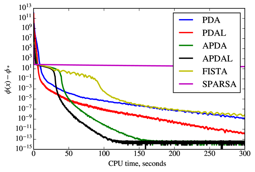
(b) Example 2

(c) Example 3

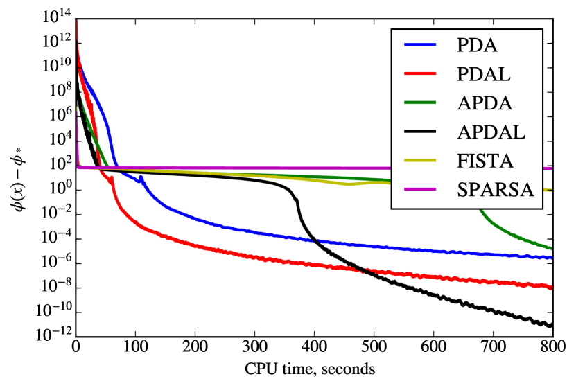
(d) Example 4

Figure 2: Convergence plots for problem (53)

5.3 Nonnegative least squares

Next, we consider another regularized least squares problem:

$$\min_{x\geq 0}\phi(x):=\frac{1}{2}\|Ax-b\|^{2},$$ (54)

where $A\in\mathbb{R}^{m\times n}$, $x\in\mathbb{R}^{n}$, $b\in\mathbb{R}^{m}$. Similarly as before, we can express it as

$$\min_{x}\max_{y}g(x)+\langle Ax,y\rangle-f^{*}y),$$ (55)

where $g(x)=\delta_{\mathbb{R}^{n}_{+}}(x)$, $f^{*}(y)=\frac{1}{2}\|y+b\|^{2}$. For all cases below we generate a random matrix $A\in\mathbb{R}^{m\times n}$ with density $d\in(0,1)$. In order to make the optimal value $\phi_{*}=0$, we always generate $w$ as a sparse vector in $\mathbb{R}^{n}$ whose $s$ nonzero entries are drawn from the uniform distribution in $[0,100]$. Then we set $b=Aw$.

We test the performance of the same algorithms as in the previous example. For FISTA and SpaRSA we use the same parameters as before. For every instance of the problem, PDA and PDAL use the same $\beta$. For APDA and APDAL we always set $\beta=1$ and $\gamma=0.1$. The initial points are $x^{0}=(0,\dots,0)$ and $y^{0}=Ax^{0}-b=-b$.

We generate our data as follows:

1. $m=2000$, $n=4000$, $d=1$, $s=1000$; the entries of $A$ are generated independently from the uniform distribution in $[-1,1]$. $\beta=25$.

2. $m=1000$, $n=2000$, $d=0.5$, $s=100$; the nonzero entries of $A$ are generated independently from the uniform distribution in $[0,1]$. $\beta=25$.

3. $m=3000$, $n=5000$, $d=0.1$, $s=100$; the nonzero entries of $A$ are generated independently from the uniform distribution in $[0,1]$. $\beta=25$.

4. $m=10000$, $n=20000$, $d=0.01$, $s=500$; the nonzero entries of $A$ are generated independently from the normal distribution $\mathcal{N}(0,1)$. $\beta=1$.

As (54) is again just a regularized least squares problem, the linesearch does not require any additional matrix-vector multiplications. The results with $\phi(x^{k})-\phi_{*}$ vs. CPU time are presented in Figure 3.

(a) Example 1

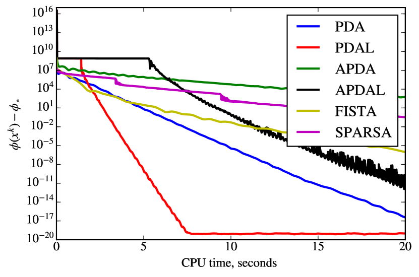
(b) Example 2

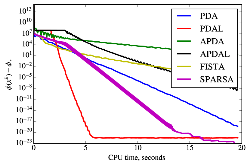
(c) Example 3

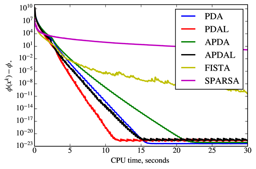
(d) Example 4

Figure 3: Convergence plots for problem (54)

Although primal-dual methods may converge faster, they require tuning $\beta=\sigma/\tau$. It is also interesting to highlight that sometimes non-accelerated methods with a properly chosen ratio $\sigma/\tau$ can be faster than their accelerated variants.

6 Conclusion

In this work, we have presented several primal-dual algorithms with linesearch. On the one hand, this allows us to avoid the evaluation of the operator norm, and on the other hand, it allows us to make larger steps. The proposed linesearch is very simple and in many important cases it does not require any additional expensive operations (such as matrix-vector multiplications or prox-operators). For all methods we have proved convergence. Our experiments confirm the numerical efficiency of the proposed methods.

Acknowledgements: The work is supported by the Austrian science fund (FWF) under the project "Efficient Algorithms for Nonsmooth Optimization in Imaging" (EANOI) No. I1148. The authors also would like to thank the referees and the SIOPT editor Wotao Yin for their careful reading of the manuscript and their numerous helpful comments.

References

- [1] A. Agarwal, S. Negahban, and M. J. Wainwright. Fast global convergence rates of gradient methods for high-dimensional statistical recovery. In Adv. Neur. In., pages 37–45, 2010.
- [2] H. H. Bauschke and P. L. Combettes. Convex Analysis and Monotone Operator Theory in Hilbert Spaces. Springer, New York, 2011.
- [3] A. Beck and M. Teboulle. A fast iterative shrinkage-thresholding algorithm for linear inverse problem. SIAM J. Imaging Sci., 2(1):183–202, 2009.
- [4] A. Chambolle and T. Pock. A first-order primal-dual algorithm for convex problems with applications to imaging. J. Math. Imaging. Vis., 40(1):120–145, 2011.
- [5] A. Chambolle and T. Pock. On the ergodic convergence rates of a first-order primal–dual algorithm. Math. Program., pages 1–35, 2015.
- [6] A. Chambolle and T. Pock. An introduction to continuous optimization for imaging. Acta Numerica, 25:161–319, 2016.
- [7] L. Condat. A primal–dual splitting method for convex optimization involving lipschitzian, proximable and linear composite terms. J. Optimiz. Theory App., 158(2):460–479, 2013.
- [8] J. Duchi, S. Shalev-Shwartz, Y. Singer, and T. Chandra. Efficient projections onto the -ball for learning in high dimensions. In Proceedings of the 25th international conference on Machine learning, pages 272–279, 2008.
- [9] T. Goldstein, M. Li, and X. Yuan. Adaptive primal-dual splitting methods for statistical learning and image processing. In Advances in Neural Information Processing Systems, pages 2089–2097, 2015.
- [10] T. Goldstein, M. Li, X. Yuan, E. Esser, and R. Baraniuk. Adaptive primal-dual hybrid gradient methods for saddle-point problems. arXiv preprint arXiv:1305.0546, 2013.
- [11] B. He, H. Yang, and S. Wang. Alternating direction method with self-adaptive penalty parameters for monotone variational inequalities. J. Optimiz. Theory App., 106(2):337–356, 2000.
- [12] B. He and X. Yuan. Convergence analysis of primal-dual algorithms for a saddle-point problem: From contraction perspective. SIAM J. Imag. Sci., 5(1):119–149, 2012.
- [13] N. Komodakis and J. C. Pesquet. Playing with duality: An overview of recent primal-dual approaches for solving large-scale optimization problems. IEEE Signal Proc. Mag., 32(6):31–54, 2015.
- [14] Y. Malitsky. Reflected projected gradient method for solving monotone variational inequalities. SIAM J. Optimiz., 25(1):502–520, 2015.
- [15] Y. Malitsky. Proximal extrapolated gradient methods for variational inequalities. Optimization Methods and Software, 33(1):140–164, 2018.
- [16] T. Pock and A. Chambolle. Diagonal preconditioning for first order primal-dual algorithms in convex optimization. In Computer Vision (ICCV), 2011 IEEE International Conference on, pages 1762–1769. IEEE, 2011.
- [17] P. Tseng. A modified forward-backward splitting method for maximal monotone mappings. SIAM J. Control, 38:431–446, 2000.
- [18] B. C. Vũ. A splitting algorithm for dual monotone inclusions involving cocoercive operators. Advances in Computational Mathematics, 38(3):667–681, 2013.
- [19] S. J. Wright, R. D. Nowak, and M. A. Figueiredo. Sparse reconstruction by separable approximation. IEEE Transactions on Signal Processing, 57(7):2479–2493, 2009.