Minicharged particles search by strong laser pulse-induced vacuum polarization effects

Abstract

Laser-based searches of the yet unobserved vacuum birefringence might be sensitive for very light hypothetical particles carrying a tiny fraction of the electron charge. We show that, with the help of contemporary techniques, polarimetric investigations driven by an optical laser pulse of moderate intensity might allow for excluding regions of the parameter space of these particle candidates which have not been discarded so far by laboratory measurement data. Particular attention is paid to the role of a Gaussian wave profile. It is argued that, at energy regimes in which the vacuum becomes dichroic due to these minicharges, the transmission probability of a probe beam through an analyzer set crossed to the initial polarization direction will depend on both the induced ellipticity as well as the rotation of the initial polarization plane. The weak and strong field regimes, relative to the attributes of these minicharged particles, and the relevance of the polarization of the strong field are investigated.

1 Introduction

The Standard Model of particle physics is currently understood as an effective theory, where charge quantization seems to be conceived as a fundamental principle. Standard Model extensions–which are required for other reasons–can be found either by enforcing the mentioned quantization through higher gauge groups or by incorporating carriers of a tiny charge $\mathpzc{q}_{\epsilon}=\epsilon|e|$, with $\epsilon$ denoting the parameter relative to the absolute value of the electron charge $e<0$ [2, 3, 4, 5, 6, 7]. That these particle candidates have eluded a direct experimental verification indicates that their interaction with the well established Standard Model branch might be extremely feeble [$\epsilon\ll 1$]. In light of this situation, the parameter space of this sort of Mini-Charged Particles (MCPs) [8, 9, 10, 11, 12, 13] is being limited. Stringent constraints have been inferred from nonobservable effects in the stellar evolution [14] [$\epsilon\lesssim 10^{-14}$ for masses $m_{\epsilon}$ below a few $\rm keV$] and the analysis of the big bang nucleosynthesis [$\epsilon<10^{-9}$ for $m_{\epsilon}<1\ \rm MeV$]. However, these astro-cosmological bounds are somewhat vulnerable due to the uncertainty associated with the underlying phenomenological model [15, 16, 17, 18]. Laboratory limits are considerably less stringent but more reliable. They have been established from regeneration setups [19, 20, 21, 22, 23, 24, 25], tests for modifications in Coulomb’s law [27, 28] or through high precision experiments looking for magnetically-induced vacuum birefringence and vacuum dichroism [29, 30, 31, 32, 33]. In the last scenario the bound is the more stringent the greater the field strength and its spatial extension are. However, in laboratories, the highest constant magnetic fields do not exceed values of the order of $\sim 10^{6}\ \mathrm{G}$, which are extended over effective distances of upto $10-100$ kilometers using Fabry-Pérot cavities.

Fields generated from high-intensity lasers might be beneficial for these laboratory searches. Indeed, the chirped-pulse amplification technique has enabled us to reach very strong magnetic field strengths, at the expense of being distributed inhomogeneously over regions of only a few micrometers [38]. Strengths as large as $\sim 10^{9}\ \rm G$ are accessible nowadays and will likely exceed values of the order of $\sim 10^{11}\ \rm G$ at forthcoming laser systems such as ELI and XCELS [39, 40]. This fact also justifies why high-intensity laser pulses are currently considered as valuable instruments for detecting various nonlinear phenomena that have eluded their observation so far. Notably, to measure vacuum birefringence [41, 42, 43, 44, 45], the HIBEF consortium has proposed a laser-based polarimetric experiment which combines a Petawatt optical laser with a x-ray free electron laser [46, 47]. Meanwhile, alternative setups are being proposed for improving the levels of sensitivity necessary for the detection of this elusive phenomenon [48, 49, 50, 51]. Clearly, experiments of this nature might also constitute sensitive probes for axion-like particles [52, 53, 54, 55, 56], MCPs and paraphotons [57, 58, 59, 60]. This forms the main motivation for this work. In this Letter we show that a polarimetric probe driven by the field of a high intensity linearly polarized Gaussian laser pulse might notably improve the existing laboratory limits in some regions of the parameter space of MCPs.

Our investigation relies on the one-loop representation of the polarization tensor in a plane-wave background [61, 62, 63] in which the two-point correlation function for MCPs incorporates the field of the laser pulse in a nonpertubative way [Furry picture]. The weak and strong field regimes, relative to the attributes of these degrees of freedom, are investigated and asymptotic expressions for the observables are derived [see Sec. 3 for more details]. In the weak field case, dispersive effects are found to be maximized at the threshold of pair production of MCPs, in agreement with the cross section of light-by-light scattering. Finally, a comparison between the present results and those previously obtained for a circularly polarized monochromatic plane-wave background [58, 59] is established.

2 Photon propagation in MCPs vacuum

We wish to evaluate the effects induced by quantum vacuum fluctuations dominated by Dirac fields characterized by a mass $m_{\epsilon}$ and a tiny fraction of the absolute value of the electron charge $\mathpzc{q}_{\epsilon}\equiv\epsilon|e|$. As long as such fields are minimally coupled to an electromagnetic field and the corresponding functional action preserves the formal invariance properties of Quantum Electrodynamics (QED), the underlying theory would resemble the corresponding phenomenology. Accordingly, the equation of motion–up to linear terms in the small-amplitude wave $a_{\mu}(x)$–has the form

$$\square a_{\mu}(x)+\int d^{4}x^{\prime}\Pi_{\mu\nu}(x,x^{\prime})a^{\nu}(x^{\prime})=0,$$ (1)

provided the Lorenz gauge $\partial_{\mu}a^{\mu}=0$ is chosen. Here, $\square\equiv\partial_{\mu}\partial^{\mu}=\partial^{2}/\partial t^{2}-\nabla^{2}$, whereas the second term in Eq. (1) introduces the vacuum polarization tensor $\Pi_{\mu\nu}(x,x^{\prime})$. This object is basically the same as in QED, with the positron parameters $(|e|,\ m)$ substituted by the respective quantities associated with the MCP $(\mathpzc{q}_{\epsilon},\ m_{\epsilon})$. It constitutes the lowest nontrivial one-particle irreducible vertex from which the gauge sector of QED can acquire a dependence on the external background field. Its four-potential is taken hereafter as

$$\mathscr{A}^{\mu}(x)=\mathpzc{a}^{\mu}_{1}\psi_{1}(\varphi)+\mathpzc{a}^{\mu}_{2}\psi_{2}(\varphi),$$ (2)

where $\mathpzc{a}_{1,2}$ are two orthogonal amplitude vectors [$\mathpzc{a}_{1}\mathpzc{a}_{2}=0$] and $\psi_{1,2}(\varphi)$ arbitrary functions of the strong plane-wave phase $\varphi=\varkappa x$. The external potential is chosen in the Lorenz gauge $\partial_{\mu}\mathscr{A}^{\mu}=0$ so that the wave four-vector $\varkappa^{\mu}=(\varkappa^{0},\boldsymbol{\varkappa})$ with $\varkappa^{2}=0$ and the amplitude vectors $\mathpzc{a}_{1,2}^{\mu}$ satisfy the constraints $\varkappa\mathpzc{a}_{1,2}=0$.

At this point, it turns out to be rather useful to introduce the four-vectors [61]

$$\Lambda_{1,2}^{\mu}(q)=-\frac{\mathscr{F}_{1,2}^{\mu\nu}q_{\nu}}{\varkappa q\sqrt{-\mathpzc{a}_{1,2}^{2}}},\quad\Lambda_{3,4}^{\mu}(q_{1,2})=\frac{\varkappa_{\mu}q_{1,2}^{2}-q_{1,2}^{\mu}(q\varkappa)}{\varkappa q\sqrt{q_{1,2}^{2}}},$$ (3)

which are built up from the amplitudes of the external field modes $\mathscr{F}^{\mu\nu}_{i}=\varkappa^{\mu}\mathpzc{a}^{\nu}_{i}-\varkappa^{\nu}\mathpzc{a}^{\mu}_{i}$ [$i=1,2$], the respective incoming and outgoing four-momenta of the probe photons $q_{1}$ and $q_{2}$ as well as the wave four-vector $\varkappa$. We note that the shorthand notation $q$ in Eq. (3) may stand for either $q_{1}$ or $q_{2}$ due to momentum conservation. The set of four-vectors $q_{1}$, $\Lambda_{1}(q_{1})$, $\Lambda_{2}(q_{1})$ and $\Lambda_{3}(q_{1})$, form a complete orthonormalized basis, i.e., $\Lambda_{i}^{\mu}(q_{1})\Lambda_{j\mu}(q_{1})=-\delta_{ij}$, $\mathpzc{g}^{\mu\nu}=q_{1}^{\mu}q_{1}^{\nu}/q_{1}^{2}-\sum_{i=1}^{3}\Lambda_{i}^{\mu}(q_{1})\Lambda_{i}^{\nu}(q_{1})$ with $\mathpzc{g}_{\mu\nu}=\mathrm{diag}(+1,-1,-1,-1)$ denoting the metric tensor. A similar statement applies to the set of four-vectors $q_{2}$, $\Lambda_{1}(q_{2}),$ $\Lambda_{2}(q_{2})$ and $\Lambda_{4}(q_{2})$.

Let us proceed by Fourier transforming Eq. (1). In the following we will seek the solutions of the resulting equation in the form of a superposition of transverse waves $a^{\mu}(q)=\sum_{i=1,2}\Lambda^{\mu}_{i}(q)f_{i}(q)$. Correspondingly,

$$\begin{split}&q_{2}^{2}f_{i}(q_{2})=-\sum_{j=1,2}\int{\mathchar 22\relax\mkern-12.0mud}^{4}q_{1}\Lambda_{i}^{\mu}(q_{2})\Pi_{\mu\nu}(-q_{2},-q_{1})\Lambda^{\nu}_{j}(q_{1})f_{j}(q_{1}),\\ &\Pi_{\mu\nu}(q_{1},q_{2})=\frac{{\mathchar 22\relax\mkern-7.5mu\delta}_{q_{2},q_{1}}}{\varkappa_{+}}\int d\varphi\mathpzc{P}_{\mu\nu}(\varphi,q_{1},q_{2})\exp\left[\frac{i(q_{2}-q_{1})_{+}}{\varkappa_{+}}\varphi\right],\end{split}$$ (4)

where we have introduced the shorthand notations $\quad{\mathchar 22\relax\mkern-12.0mud}\equiv d/(2\pi)$ and $\quad{\mathchar 22\relax\mkern-7.5mu\delta}_{q_{2},q_{1}}\equiv(2\pi)^{3}\delta^{(\perp)}(q_{2}-q_{1})\delta^{(-)}(q_{2}-q_{1})$. Note that quantities with subindices $\pm$ and $\perp$ refer to light-cone coordinates. We choose the reference frame in such a way that the direction of propagation of our external plane wave [see Eq. (2)] is along the positive direction of the third axis. As a consequence, the strong field only depends on $x_{-}=(x^{0}-x^{3})/\sqrt{2}$ via $\varphi=\varkappa_{+}x_{-}$ with $\varkappa_{+}=(\varkappa^{0}+\varkappa^{3})/\sqrt{2}=\sqrt{2}\varkappa_{0}>0$ and the remaining light-cone variables, i.e. $x_{+}=(x^{0}+x^{3})/\sqrt{2}$ and $\boldsymbol{x}_{\perp}=(x^{1},x^{2})$ can be integrated out without complications.

Although the expression above holds for arbitrary external field profiles, it still requires a transversely homogeneous field. As a consequence, $\boldsymbol{q}_{\perp}$ is conserved [see the associated Dirac delta in Eq. (4)], which constitutes a good approximation whenever the Compton wavelength of the MCP ${\mkern 0.75mu\mathchar 22\relax\mkern-9.75mu\lambda}_{\epsilon}=1/m_{\epsilon}$ becomes much smaller than the transverse length scale over which the field is homogeneous. For a focused laser beam this scale is set by the waist size of the pulse $w_{0}$. Therefore, the plane-wave approximation is valid in the regime $m_{\epsilon}\gg w_{0}^{-1}$. The study of the regime $m_{\epsilon}\lesssim w_{0}^{-1}$, where spatial focusing effects become important, is beyond the scope of the present investigation.

The tensorial structure of $\mathpzc{P}_{\mu\nu}(\varphi,q_{1},q_{2})$ can be determined on the basis of symmetry principles, independently of any approximation used to compute the polarization tensor [61, 63]. It reads

$$\begin{split}&\mathpzc{P}^{\mu\nu}(\varphi,q_{1},q_{2})=c_{1}\Lambda^{\mu}_{1}\Lambda^{\nu}_{2}+c_{2}\Lambda^{\mu}_{2}\Lambda^{\nu}_{1}+c_{3}\Lambda^{\mu}_{1}\Lambda^{\nu}_{1}\\ &\qquad\qquad\qquad\qquad\qquad\qquad\quad+c_{4}\Lambda^{\mu}_{2}\Lambda^{\nu}_{2}+c_{5}\Lambda^{\mu}_{3}\Lambda^{\nu}_{4}.\end{split}$$ (5)

As $q_{1}-q_{2}\sim\varkappa$ this decomposition does not depend on which choice of $q$ is taken; see also Eq. (3). The form factors $c_{i}$ in Eq. (5) depend–among other parameters–on the phase of the external field $\varphi$, $q_{1}$ and $q_{2}$. In the one-loop approximation–which is adopted from now on–they turn out to be represented by two-fold parametric integrals in the variables $\tau\in[0,\infty)$ and $v\in[0,1]$, the integrand of which being of the form [see Ref. [61]]

$$\exp[-im_{\epsilon}^{2}\tau+i\mu q_{1}^{2}]\times\left(\mathrm{Regular}\ \mathrm{Function}\ \mathrm{in}\ q_{1}^{2},\ q_{2}^{2}\ \mathrm{and}\ \varkappa q\right)$$ (6)

with $\mu=\frac{1}{4}\tau(1-v^{2})$. After a suitable integration by parts the regular function becomes independent of $q_{2}^{2}$ [see Ref. [64], App. D for more details], which is assumed in the following.

When polarization effects do not dramatically modify the photon dispersion law in vacuum [$q^{2}=0$], one can solve Eq. (4) perturbatively by setting $f_{i}(q)\approx f_{0i}(q)+\delta f_{i}(q)$. In the following, we suppose a head-on collision between the strong laser pulse and the probe beam characterized by the four-momentum $k^{\mu}=(\omega_{\boldsymbol{k}},\boldsymbol{k})$, so that $\varkappa_{+}k_{-}=2\omega_{\boldsymbol{k}}\varkappa_{0}$ and $\boldsymbol{k}_{\perp}=\boldsymbol{0}$. Accordingly, the leading order term is $f_{0i}(q)=|2q_{-}|a_{0i}\ {\mathchar 22\relax\mkern-7.5mu\delta}(q^{2})\ {\mathchar 22\relax\mkern-7.5mu\delta}^{(\perp)}(q)\ {\mathchar 22\relax\mkern-7.5mu\delta}^{(-)}(q-k)$, corresponding to $f_{0i}(x)=a_{0i}e^{-i\phi}$ with $\phi=kx=k_{-}x_{+}$ and $a_{0i}$ the amplitude of mode-$i$. Then, it follows from Eq. (4) that the perturbative contribution is given by

$$\begin{split}&\delta f_{i}(q_{2})=-[2q_{2+}q_{2-}-q_{2\perp}^{2}+i0]^{-1}\\ &\qquad\qquad\qquad\qquad\times\sum_{j=1,2}a_{0j}\Lambda_{j}^{\mu}(k)\Pi_{\mu\nu}(k,q_{2})\Lambda^{\nu}_{i}(q_{2}),\end{split}$$ (7)

where it must be understood that the only nonvanishing light-cone component of the four-vector $k^{\mu}$ is $k_{-}$. Besides, in obtaining the expression above we have used the symmetry property $\Pi_{\mu\nu}(-q_{2},-q_{1})=\Pi_{\nu\mu}(q_{1},q_{2})$. Here, the poles in the function $1/q_{2}^{2}$ have been shifted infinitesimally into the complex plane by an $i0$-term so that correct boundary conditions of the fields at asymptotic times $f_{i}(\pm\infty,\boldsymbol{x})$ are implemented. In this case, the solution of Eq. (1) is given by $a^{\mu}(x)=\sum_{i=1,2}\Lambda_{i}^{\mu}(k)f_{i}(x)$ [see above Eq. (4)] with

$$\begin{split}&f_{i}(x)\approx f_{0i}(x)-\frac{1}{2\varkappa_{+}k_{-}}\sum_{j=1,2}f_{0j}(x)\int d\tilde{\varphi}\int{\mathchar 22\relax\mkern-12.0mud}q_{2+}\\ &\quad\qquad\qquad\times e^{\frac{iq_{2+}}{\varkappa_{+}}(\tilde{\varphi}-\varphi)}\Lambda_{j}^{\mu}(k)\frac{\mathpzc{P}_{\mu\nu}(\tilde{\varphi},k,q_{2})}{q_{2+}+i0}\Lambda^{\nu}_{i}(q_{2}).\end{split}$$ (8)

Here, $q_{2-}=k_{-}$, $\boldsymbol{q}_{2\perp}=\boldsymbol{0}$, whereas $\boldsymbol{k}_{\perp}=\boldsymbol{0}$ and $k_{+}=0$. In order to provide a more concise expression for $f_{i}(x)$, we integrate out $q_{2+}$. This can be carried out by applying Cauchy’s theorem and the residue theorem, depending upon whether the contour of integration is chosen in the upper or lower half of the complex plane. Taking into account the structure of the integrand with respect to $q_{2+}$ [see Eq. (6) and the discussion below], we obtain

$$\int{\mathchar 22\relax\mkern-12.0mud}q_{2+}\ldots=-i\Lambda_{j}^{\mu}(k)\mathpzc{P}_{\mu\nu}(\tilde{\varphi},k,k)\Lambda^{\nu}_{i}(k)\Theta(\varphi-\tilde{\varphi}),$$ (9)

where $\Theta(x)$ denotes the unit step function. Its emergence restricts the integral over $\tilde{\varphi}$ to $(-\infty,\varphi]$ instead of $(-\infty,\infty)$, as required by causality. However, we are only interested in asymptotically large spacetime distances [$\varphi\to\infty$], i.e., when the high-intensity laser field is turned off, which restores the original integration limits. Therefore, inserting this expression into Eq. (8) and taking into account the tensorial decomposition of the polarization tensor [see Eq. (5)], we end up with

$$\begin{split}&f_{i}(x)\approx f_{0i}(x)+\frac{i}{2\varkappa_{+}k_{-}}f_{01}(x)\int_{-\infty}^{\varphi}d\tilde{\varphi}\left[c_{3}(\tilde{\varphi})\delta_{i1}+c_{1}(\tilde{\varphi})\delta_{i2}\right]\\ &\qquad\qquad+\frac{i}{2\varkappa_{+}k_{-}}f_{02}(x)\int_{-\infty}^{\varphi}d\tilde{\varphi}\left[c_{4}(\tilde{\varphi})\delta_{i2}+c_{2}(\tilde{\varphi})\delta_{i1}\right].\end{split}$$ (10)

The expression above constitutes the starting point for further considerations. It holds for arbitrary strength and polarization of the background field, as long as the vacuum polarization is small. When specifying Eq. (10) to the case of a linearly polarized plane-wave background, i.e. Eq. (2) with $\psi_{2}(\varphi)=0$, the form factors $c_{1,2}$ vanish [61, 63] and the resulting expression agrees with Eq. (16) in Ref. [64], provided the involved exponential function is expanded to leading order. However, we emphasize that the aforementioned solution has been established for the field regime in which the laser intensity parameter $\xi=|e|\sqrt{-\mathpzc{a}^{2}}/m$ with $\mathpzc{a}^{\mu}\equiv\mathpzc{a}_{1}^{\mu}$ is very large [$\xi\gg 1$].

Now, if the external field is linearly polarized, the solution of Eq. (10) allows us to write the electric field of the probe [$\boldsymbol{\varepsilon}(x)=-\partial\boldsymbol{a}/\partial x^{0}$ with $a_{0}=0$] as a superposition of plane-waves

$$\begin{split}&\boldsymbol{\varepsilon}(x)\approx\varepsilon_{0}\cos(\vartheta_{0})\boldsymbol{\Lambda}_{1}\mathrm{Re}\,e^{-i\phi+\frac{i}{2\varkappa_{+}k_{-}}\int_{-\infty}^{\varphi}d\tilde{\varphi}\ c_{3}(\tilde{\varphi})}\\ &\qquad\qquad+\varepsilon_{0}\sin(\vartheta_{0})\boldsymbol{\Lambda}_{2}\mathrm{Re}\,e^{-i\phi+\frac{i}{2\varkappa_{+}k_{-}}\int_{-\infty}^{\varphi}d\tilde{\varphi}\ c_{4}(\tilde{\varphi})}.\end{split}$$ (11)

Here, $\varepsilon_{0}$ refers to the initial electric field amplitude, $\boldsymbol{\Lambda}_{1,2}=\boldsymbol{\mathpzc{a}}_{1,2}/|\boldsymbol{\mathpzc{a}}_{1,2}|$, whereas $0\leqslant\vartheta_{0}<\pi$ is the corresponding initial polarization angle of the probe with respect to $\boldsymbol{\Lambda}_{1}$, i.e., the polarization axis of the external pulse. Observe that the appearance of the phase is due to the approximation $1+ix\approx\exp(ix)$ as in Ref. [43].

The $\mathpzc{P}_{\mu\nu}-$form factors are, in general, complex functions $c_{3,4}=\mathrm{Re}\ c_{3,4}+i\ \mathrm{Im}\ c_{3,4}$. Correspondingly, the exponents in Eq. (11) contain real and imaginary contributions. The latter are connected to the photo-production of MCP pairs via the optical theorem [64, 65], a phenomenon which damps the intensity of the probe, $I(\varphi)=\frac{\varepsilon_{0}^{2}}{4\pi}\cos^{2}(\vartheta_{0})\exp(-\kappa_{1})+\frac{\varepsilon_{0}^{2}}{4\pi}\sin^{2}(\vartheta_{0})\exp(-\kappa_{2})$, as it propagates in the pulse. As such, the analytic properties of the factors $\kappa_{1,2}\equiv\kappa_{1,2}(\varphi)=\frac{1}{\varkappa_{+}k_{-}}\mathrm{Im}\int_{-\infty}^{\varphi}d\tilde{\varphi}\ c_{3,4}(\tilde{\varphi})$, responsible for the damping differ from each other, leading to a nontrivial difference $\delta\kappa(\varphi)=\frac{1}{\varkappa_{+}k_{-}}\mathrm{Im}\ \Delta(\varphi)$, where we introduced the function

$$\Delta(\varphi)=\int_{-\infty}^{\varphi}d\tilde{\varphi}\ \left[c_{3}(\tilde{\varphi})-c_{4}(\tilde{\varphi})\right].$$ (12)

Therefore, the vacuum behaves like a dichroic medium, inducing a rotation of the probe polarization from the initial angle $\vartheta_{0}$ to $\vartheta_{0}+\delta\vartheta$, where $\delta\vartheta$ is expected to be tiny. At asymptotically large spacetime distances [$\varphi\to\infty$], we find

$$|\delta\vartheta(\epsilon,m_{\epsilon})|\approx\frac{1}{2}\sin(2\vartheta_{0})\left|\frac{\mathrm{Im}\ \Delta(\infty)}{2\varkappa_{+}k_{-}}\right|\ll 1.$$ (13)

As the phase difference between the two propagating modes, $\delta\phi(\varphi)=\frac{1}{2\varkappa_{+}k_{-}}\mathrm{Re}\ \Delta(\varphi)$, does not vanish either [see Eq. (11)], the vacuum is also predicted to be birefringent. Hence, when the strong field is turned off [$\varphi\to\infty$], the outgoing probe should be elliptically polarized and its ellipticity is given by [66] [note that in this reference a different notation is used]

$$|\psi(\epsilon,m_{\epsilon})|\approx\frac{1}{2}\sin(2\vartheta_{0})\left|\frac{\mathrm{Re}\ \Delta(\infty)}{2\varkappa_{+}k_{-}}\right|\ll 1.$$ (14)

In the case of optical probes, isolated detections of the rotation effect [see Eq. (13)] and the ellipticity [see Eq. (14)] could be carried out depending on whether a quarter wave plate is inserted or not in the path of the outgoing probe beam in front of a Faraday cell and an analyzer [29, 30, 33]. The latter is set crossed to the initial direction of polarization so that the transmitted photons are polarized orthogonally. Correspondingly, no photons are detected in the absence of birefringence and dichroism. Using high-purity polarimetric techniques for x-rays [67, 68] (QED) vacuum birefringence could also be measured with a similar setup by combining a x-ray probe and a strong optical field [QED-induced dichroism is exponentially small, thus $\delta\vartheta_{\mathrm{QED}}=0$ for practical purposes]. Such an experiment is envisaged at HIBEF [47].

In a scenario including MCPs, the analysis must be revisited. To this end, let us consider the scattering amplitude $T=i\mathpzc{e}_{\mu}^{(i)}\left[\Pi_{\mathrm{QED}}^{\mu\nu}(k_{1},k_{2})+\Pi^{\mu\nu}(k_{1},k_{2})\right]\mathpzc{e}_{\nu}^{(f)}/[2V(\omega_{\boldsymbol{k}_{1}}\omega_{\boldsymbol{k}_{2}})^{\nicefrac{{1}}{{2}}}]$. The expression above includes both, the polarization tensor associated with QED $\Pi_{\mathrm{QED}}^{\mu\nu}(k_{1},k_{2})$ and the one related to the MCPs. Besides, $V$ denotes the normalization volume, whereas $\mathpzc{e}^{(i)}_{\mu}$ and $\mathpzc{e}^{(f)}_{\mu}$ are the initial and final polarization states, respectively. Following Eq. (11), we suppose that the former is of the form $\mathpzc{e}^{(i)}=\cos(\vartheta_{0})\Lambda_{1}+\sin(\vartheta_{0})\Lambda_{2}$. In contrast, the polarization state transmitted by the analyzer is $\mathpzc{e}^{(f)}=\pm\sin(\vartheta_{0})\Lambda_{1}\mp\cos(\vartheta_{0})\Lambda_{2}$, so that $\mathpzc{e}^{(i)}\mathpzc{e}^{(f)}=0$. Finally, we establish the following expression for the transmission probability [$\delta\vartheta_{\mathrm{QED}}=0$]:

$$\begin{split}&\mathcal{P}=\left[\psi_{\mathrm{QED}}+\psi(\epsilon,m_{\epsilon})\right]^{2}+\delta\vartheta(\epsilon,m_{\epsilon})^{2}.\end{split}$$ (15)

This expression indicates that the described setup is not suitable to probe the signals separately. However, one could achieve this goal by determining the local minimum of the count rate behind the analyzer, which is no longer perpendicular to the incoming polarization direction but shifted by $\delta\vartheta(\epsilon,m_{\epsilon})$ [69]. We indeed find that in such a configuration, the transmission probability $\mathcal{P}_{\mathrm{min}}=|\boldsymbol{\mathpzc{e}}\cdot\boldsymbol{\varepsilon}|^{2}/|\varepsilon_{0}|^{2}$ with $\boldsymbol{\mathpzc{e}}=\pm\sin(\vartheta_{0}+\delta\vartheta)\boldsymbol{\Lambda}_{1}\mp\cos(\vartheta_{0}+\delta\vartheta)\boldsymbol{\Lambda}_{2}$, is given by the first term on the right-hand side of Eq. (15). In connection, the number of photons transmitted through the analyzer reads $\mathcal{N}\approx\mathcal{N}_{\mathrm{in}}\mathcal{N}_{\mathrm{shot}}\mathcal{T}\left[\psi_{\mathrm{QED}}^{2}+2\psi_{\mathrm{QED}}\psi(\epsilon,m_{\epsilon})\right]$, provided that QED effects are dominant [$\psi_{\mathrm{QED}}>\psi(\epsilon,m_{\epsilon})$]. Here, $\mathcal{N}_{\mathrm{shot}}$ counts the number of laser shots used for a measurement, $\mathcal{T}$ denotes the transmission coefficient of all optical components and $\mathcal{N}_{\rm in}$ is the number of incoming x-ray probe photons, respectively.

3 Asymptotic regimes

We wish to investigate the optical observables [Eq. (13) and (14)] induced by a plausible existence of MCPs. Since both depend on $\Delta(\infty)$ [see Eq. (12)], we will focus on determining this function. Indeed, a suitable expression can be inferred from the literature [61, 63]. In the one-loop approximation we find:

$$\begin{split}&\Delta(\infty)=\frac{\alpha_{\epsilon}}{\pi}m_{\epsilon}^{2}\xi_{\epsilon}^{2}\int_{-\infty}^{\infty}d\varphi\int_{-1}^{1}dv\\ &\qquad\qquad\qquad\times\int_{0}^{\infty}\frac{d\tau}{\tau}X(\varphi)\exp\left[-im_{*}^{2}(\varphi)\tau\right],\end{split}$$ (16)

where $\alpha_{\epsilon}\equiv\epsilon^{2}e^{2}\approx\epsilon^{2}/137$ denotes the fine structure constant relative to the MCPs, whereas $\xi_{\epsilon}=\epsilon m\xi/m_{\epsilon}$ is the relative intensity parameter. The remaining functions involved in this expression can be conveniently written in the following form

$$\begin{split}&X(\varphi)=\mu^{2}(2\varkappa_{+}k_{-})^{2}\int_{0}^{1}dy\int_{0}^{1}d\tilde{y}\ y(\tilde{y}-1)\psi^{\prime}(\varphi_{y})\psi^{\prime}(\varphi_{\tilde{y}}),\\ &m_{*}^{2}(\varphi)=m_{\epsilon}^{2}\left\{1-\xi_{\epsilon}^{2}\mu^{2}(2\varkappa_{+}k_{-})^{2}\int_{0}^{1}dy\ y\psi^{\prime}(\varphi_{y})\right.\\ &\qquad\qquad\qquad\times\left.\left[\int_{0}^{1}d\tilde{y}\ \tilde{y}\psi^{\prime}(\varphi_{\tilde{y}})-2\int_{y}^{1}d\tilde{y}\ \psi^{\prime}(\varphi_{\tilde{y}})\right]\right\},\end{split}$$ (17)

where $\mu=\frac{1}{4}\tau(1-v^{2})$ and $\varphi_{y}=\varphi-2(\varkappa_{+}k_{-})\mu y$. These expressions apply for a linearly polarized plane-wave background [$\psi_{1}(\varphi)\equiv\psi(\varphi)$ and $\psi_{2}(\varphi)=0$]. Here, the prime denotes the derivative with respect to the argument. An exact evaluation of $\Delta(\infty)$ [see Eq. (12)] is quite difficult to perform. Therefore, we consider now some asymptotic expressions of interest.

3.1 Leading behavior at large $\xi_{\epsilon}\gg 1$

In order to elucidate the asymptotic contribution of Eq. (16) at asymptotically large $\xi_{\epsilon}\gg 1$ we first perform the change of variable $\tau=4\rho/[|\varkappa_{+}k_{-}|(1-v^{2})]$. The resulting integration over $\rho$ is divided into two contributions whose domains run from $0$ to $\rho_{0}$ and from $\rho_{0}$ to $\infty$. The dimensionless parameter $\rho_{0}>0$, is chosen such that it satisfies simultaneously the conditions $\xi_{\epsilon}^{-1}\ll\rho_{0}\ll 1$ and $(\eta_{\epsilon}/\xi_{\epsilon}^{2})^{\nicefrac{{1}}{{3}}}\ll\rho_{0}$ with $\eta_{\epsilon}=\varkappa_{+}k_{-}/m_{\epsilon}^{2}$. In the former integral we Taylor expand the functions given in Eq. (17): $X(\varphi)\approx-\rho^{2}[\psi^{\prime}(\varphi)]^{2}$ and $m_{*}^{2}(\varphi)\approx m_{\epsilon}^{2}\left[1+\frac{\xi_{\epsilon}^{2}\rho^{2}}{3}[\psi^{\prime}(\varphi)]^{2}\right]$. Afterward, we perform the change of variable $s=\rho\xi_{\epsilon}$ and extend the resulting integration limit $\rho_{0}\xi_{\epsilon}\to\infty$. No relevant contribution comes from the integral defined in $[\rho_{0},\infty)$. Therefore, in the strong field regime $\xi_{\epsilon}\gg 1$ [$\eta_{\epsilon}\ll\xi_{\epsilon}^{2}$], the function $\Delta(\infty)$ [see Eq. (16)] is well approximated by

$$\Delta(\infty)=-\alpha_{\epsilon}m_{\epsilon}^{2}\int_{-\infty}^{\infty}d\varphi\int_{-1}^{1}dv\left[\frac{\mathrm{Gi}^{\prime}(x)}{x}+i\frac{\mathrm{Ai}^{\prime}(x)}{x}\right].$$ (18)

Here, $x=\left(6/[|\zeta_{\epsilon}(\varphi)|(1-v^{2})]\right)^{\nicefrac{{2}}{{3}}}$, $\mathrm{Gi}(x)$ and $\mathrm{Ai}(x)$ are the Scorer and Airy functions of first kind [70], respectively. In this context, $\zeta_{\epsilon}(\varphi)=3\chi_{\epsilon}\psi^{\prime}(\varphi)/2$, with $\chi_{\epsilon}=\xi_{\epsilon}\eta_{\epsilon}$, refers to the pulse-modulated nonlinear parameter associated with the MCP vacuum.

We proceed our analysis by inserting the imaginary part of Eq. (18) into Eq. (13). As a consequence of the relation $\mathrm{Ai}^{\prime}(z)=-\frac{z}{\pi\sqrt{3}}K_{\nicefrac{{2}}{{3}}}\left(\frac{2}{3}z^{{\nicefrac{{3}}{{2}}}}\right)$, with a modified Bessel function $K_{\nu}(z)$ [70], the following representation for the rotation angle is found

$$\begin{split}&|\delta\vartheta(\epsilon,m_{\epsilon})|\approx\frac{1}{2}\sin(2\vartheta_{0})\frac{\alpha_{\epsilon}m_{\epsilon}^{2}}{\sqrt{3}\pi(\varkappa_{+}k_{-})}\\ &\qquad\qquad\qquad\times\left|\int_{-\infty}^{\infty}d\varphi\int_{0}^{1}dv\ K_{\nicefrac{{2}}{{3}}}\left(\frac{4}{|\zeta_{\epsilon}(\varphi)|}\frac{1}{1-v^{2}}\right)\right|.\end{split}$$ (19)

Likewise, by substituting the real part of Eq. (18) into Eq. (14), we find for the ellipticity

$$\begin{split}&|\psi(\epsilon,m_{\epsilon})|\approx\frac{1}{2}\sin(2\vartheta_{0})\frac{\alpha_{\epsilon}m_{\epsilon}^{2}}{6^{\nicefrac{{2}}{{3}}}(\varkappa_{+}k_{-})}\left|\int_{-\infty}^{\infty}d\varphi\ |\zeta_{\epsilon}(\varphi)|^{\nicefrac{{2}}{{3}}}\right.\\ &\qquad\qquad\times\left.\int_{0}^{1}dv(1-v^{2})^{\nicefrac{{2}}{{3}}}\mathrm{Gi}^{\prime}\left[\left(\frac{6}{|\zeta_{\epsilon}(\varphi)|}\frac{1}{1-v^{2}}\right)^{\nicefrac{{2}}{{3}}}\right]\right|.\end{split}$$ (20)

Eqs. (19) and (20) are used in the next section to estimate the projected bounds in the parameter space of MCPs. Note that a numerical comparison between these expressions and the corresponding ones resulting from Eqs. (13), (14) and (16) agrees within a few percent whenever $\xi_{\epsilon}\gg 1$ and $\zeta_{\epsilon}^{\nicefrac{{1}}{{3}}}\ll\xi_{\epsilon}$, in agreement with the conditions imposed above Eq. (18).

In addition, further insights can be gained by restricting $\zeta_{\epsilon}=3\chi_{\epsilon}/2$ to some asymptotic limits. We start with the case $\zeta_{\epsilon}\ll 1$. To be consistent with $\xi_{\epsilon}\gg 1$ the parameter $\eta_{\epsilon}$ must be restricted to $\eta_{\epsilon}\ll 2/(3\xi_{\epsilon})$. In this limit we can exploit the asymptotes $K_{\nu}(z)\sim\sqrt{\frac{\pi}{2z}}e^{-z}$ and $\mathrm{Gi}(z)\sim\frac{1}{\pi z}$ [70]. With these approximations, the integrations over $v$ can be performed in both observables. The expression for the ellipticity becomes particularly simple and can be computed exactly. Conversely, the calculation of the integral contained in the rotation angle requires additional approximations. To this end, we first apply the change of variable $w=\left(1-v^{2}\right)^{-1}$ and note that the region $w\sim 1$ provides the essential contribution. This leads to

$$\begin{split}&|\delta\vartheta(\epsilon,m_{\epsilon})|\approx\frac{1}{2}\sin(2\vartheta_{0})\frac{\alpha_{\epsilon}m_{\epsilon}^{2}}{8\sqrt{6}(\varkappa_{+}k_{-})}\int_{-\infty}^{\infty}d\varphi\ |\zeta_{\epsilon}(\varphi)|e^{-\frac{4}{|\zeta_{\epsilon}(\varphi)|}},\\ &|\psi(\epsilon,m_{\epsilon})|\approx\frac{1}{2}\sin(2\vartheta_{0})\frac{2\alpha_{\epsilon}m_{\epsilon}^{2}}{135\pi(\varkappa_{+}k_{-})}\int_{-\infty}^{\infty}d\varphi\ |\zeta_{\epsilon}(\varphi)|^{2}.\end{split}$$ (21)

The situation is different when $\xi_{\epsilon}\gg\zeta_{\epsilon}^{\nicefrac{{1}}{{3}}}\gg 1$. In this case, $K_{\nu}(z)\sim\frac{\Gamma(\nu)}{2}\left(\frac{2}{z}\right)^{\nu}$ and $\mathrm{Gi}(z)\sim\frac{1}{2\pi\ 3^{\nicefrac{{2}}{{3}}}}\Gamma\left(\frac{1}{3}\right)+\frac{1}{2\pi\ 3^{\nicefrac{{1}}{{3}}}}\Gamma\left(\frac{2}{3}\right)z$ applies [70]:

$$\begin{split}&|\delta\vartheta(\epsilon,m_{\epsilon})|\approx\sqrt{3}|\psi(\epsilon,m_{\epsilon})|,\\ &|\psi(\epsilon,m_{\epsilon})|\approx\frac{1}{2}\sin(2\vartheta_{0})\frac{2^{\nicefrac{{1}}{{3}}}\alpha_{\epsilon}m_{\epsilon}^{2}\Gamma^{2}(\frac{2}{3})}{7\sqrt{\pi}(\varkappa_{+}k_{-})\Gamma(\frac{1}{6})}\left|\int_{-\infty}^{\infty}d\varphi\ |\zeta_{\epsilon}(\varphi)|^{\nicefrac{{2}}{{3}}}\right|,\end{split}$$ (22)

where $\Gamma(x)$ denotes the Gamma function. We remark that, if the external background is a constant crossed field [$\psi^{\prime}(\varphi)=1$] which extends over $\Delta x_{-}$, the ellipticity in Eq. (21) agrees with Eq. (50) in Ref. [43], provided the distance traveled by the probe is given by $d=\sqrt{2}\Delta x_{-}$ and $\vartheta_{0}=\pi/4$.

So far, no restriction has been imposed on the field profile function $\psi^{\prime}(\varphi)$. To proceed further, we take it of the form

$$\psi^{\prime}(\varphi)=e^{-\frac{\varphi^{2}}{2\Delta\varphi^{2}}}\sin(\varphi).$$ (23)

Here, $\Delta\varphi=\pi\mathpzc{N}\,/\sqrt{2\ln(2)}$ with $\mathpzc{N}$ referring to the number of oscillation cycles within the Gaussian envelop (FWHM). We insert this function into the expression for the ellipticity [see Eq. (21)] to establish

$$|\psi(\epsilon,m_{\epsilon})|\approx\frac{1}{2}\sin(2\vartheta_{0})\frac{\alpha_{\epsilon}m_{\epsilon}^{2}\zeta_{\epsilon}^{2}\Delta\varphi}{135\sqrt{\pi}(\varkappa_{+}k_{-})}\left[1-e^{-\Delta\varphi^{2}}\right].$$ (24)

The expression given in Eq. (24) is valid if simultaneously $\xi_{\epsilon}\gg 1$ and $\zeta_{\epsilon}\ll 1$. For $\xi_{\epsilon}=10$, $\zeta_{\epsilon}=0.15$ [$\zeta_{\epsilon}=3/2$] and $\Delta\varphi=4\pi$, it differs from the exact formula Eq. (14)–with Eqs. (16) and (17) included–by only $0.2\%$ [$13\%$].

The integrals which remain in $|\delta\vartheta(\epsilon,m_{\epsilon})|$ [see Eq. (21)] cannot be computed analytically. To approximate them, we write

$$\int_{-\infty}^{\infty}d\varphi\ldots=2\zeta_{\epsilon}\sum_{n=1}^{\infty}(-1)^{n-1}\int_{(n-1)\pi}^{n\pi}d\varphi\ \psi^{\prime}(\varphi)e^{\frac{4}{\zeta_{\epsilon}}\frac{(-1)^{n}}{\psi^{\prime}(\varphi)}},$$

assume that $\zeta_{\epsilon}\ll 1$, and apply the Laplace method. To this end we first note that the integrands vanish at the boundaries and that the main contributions in the series arise from those values of $\varphi$ which satisfy the condition $(n-1)\pi<\varphi<n\pi<\sqrt{2}\Delta\varphi$. Therefore, the series can be cut off at $N_{\mathrm{max}}=\lfloor 1+\mathpzc{N}\,/\ln(2)\rfloor$, where $\lfloor x\rfloor$ refers to the integer value of $x$. In addition, for the stationary points the condition $\Delta\varphi^{2}/\varphi\gg 1$ applies. Hence, we can use the approximation $\varphi\approx(2n-1)\pi/2$ with $n\in\mathbb{N}$. As a consequence,

$$\int_{-\infty}^{\infty}d\varphi\ldots\approx 2\zeta_{\epsilon}^{\nicefrac{{3}}{{2}}}\sqrt{\frac{\pi}{2}}\ \sum_{n=1}^{N_{\mathrm{max}}}\frac{1}{\gamma_{n}}e^{-\frac{4}{\zeta_{\epsilon}}\gamma_{n}},$$ (25)

with the parameter $\gamma_{n}=\exp[(2n-1)^{2}\pi^{2}/(8\Delta\varphi^{2})]$. We insert this approximation into $|\delta\vartheta(\epsilon,m_{\epsilon})|$ [see Eq. (21)] and assume $\mathpzc{N}\approx 5$. Then, the main contribution arises from the first term of the series above. Explicitly,

$$|\delta\vartheta(\epsilon,m_{\epsilon})|\approx\frac{1}{2}\sin(2\vartheta_{0})\frac{1}{8}\frac{\alpha_{\epsilon}m_{\epsilon}^{2}\zeta_{\epsilon}^{\nicefrac{{3}}{{2}}}}{(\varkappa_{+}k_{-})}\sqrt{\frac{\pi}{3}}\frac{1}{\gamma_{1}}e^{-\frac{4}{\zeta_{\epsilon}}\gamma_{1}}.$$ (26)

This result provides evidence that the photo-production probability of a pair of MCPs is suppressed as $\sim\exp(-4\gamma_{1}/\zeta_{\epsilon})$, whenever $\xi_{\epsilon}\gg 1$ and $\zeta_{\epsilon}\ll 1$. This is expected because the damping factors of the probe $\kappa_{1,2}$ [see above Eq. (12)] represent the probability of producing a pair from the respective propagating mode [64].

The integration which remains in Eq. (22) can be estimated by replacing the periodic term $|\sin(\varphi)|^{\nicefrac{{2}}{{3}}}$ by its average value, $\langle|\sin(\varphi)|^{\nicefrac{{2}}{{3}}}\rangle=3\sqrt{\frac{3}{\pi}}\frac{\Gamma(\frac{2}{3})}{\Gamma(\frac{1}{6})}$. Correspondingly, the ellipticity [rotation angle] acquires the form

$$\begin{split}&|\psi(\epsilon,m_{\epsilon})|\approx\frac{1}{2}\sin(2\vartheta_{0})\frac{18}{7\sqrt{\pi}}\frac{\alpha_{\epsilon}m_{\epsilon}^{2}}{(\varkappa_{+}k_{-})}\frac{\Gamma^{3}(\frac{2}{3})}{\Gamma^{2}(\frac{1}{6})}\left(\frac{\zeta_{\epsilon}}{2}\right)^{\nicefrac{{2}}{{3}}}\Delta\varphi,\\ &|\delta\vartheta(\epsilon,m_{\epsilon})|\approx\sqrt{3}|\psi(\epsilon,m_{\epsilon})|.\end{split}$$ (27)

These analytical results were derived by assuming that $\xi_{\epsilon}\gg\zeta_{\epsilon}^{1/3}\gg 1$. The expression for the ellipticity [rotation angle] given in Eq. (27) agrees with Eq. (20) [Eq. (19)] within an accuracy of $<19\%$ [$<3\%$] if $\zeta_{\epsilon}>10^{3}$ for $\Delta\varphi=4\pi$.

Some comments are in order. First of all, while Eq. (24) is exact with respect to the integration over $\varphi$, the approximations used to obtain Eqs. (26) and (27) prevent us from taking the monochromatic limit [$\Delta\varphi\to\infty$] directly. Instead, this limiting case can be derived by noting that the integrands in $|\delta\vartheta(\epsilon,m_{\epsilon})|$ [see Eq. (21) and Eq. (22)] are $\pi$-periodic. In this situation, we have $\int_{-\infty}^{\infty}d\varphi\ldots=2N\int_{0}^{\pi}d\varphi\ldots$ with $N\to\infty$ and thus,

$$\int_{-\infty}^{\infty}d\varphi\ldots=2\pi N\left\{\begin{array}[]{cc}\displaystyle\frac{1}{\sqrt{2\pi}}\zeta_{\epsilon}^{\nicefrac{{3}}{{2}}}e^{-\frac{4}{\zeta_{\epsilon}}}&\zeta_{\epsilon}\ll 1\\ \\ \displaystyle\left\langle|\sin(\varphi)|^{\nicefrac{{2}}{{3}}}\right\rangle&\zeta_{\epsilon}\gg 1,\end{array}\right.$$

where the result for $\zeta_{\epsilon}\ll 1$ has been quoted from Ref. [64]. Hence, we only need to carry out the respective replacements $\exp(-4\gamma_{1}/\zeta_{\epsilon})/\gamma_{1}\to Ne^{-\frac{4}{\zeta_{\epsilon}}}$ and $\Delta\varphi\to 2N\sqrt{\pi/3}$ in Eqs. (26) and (27), to establish the asymptotic behaviors of $|\delta\vartheta(\epsilon,m_{\epsilon})|$ and $|\psi(\epsilon,m_{\epsilon})|$ in the monochromatic limit.

3.2 Leading behavior at weak fields $\xi_{\epsilon}\ll 1$

In the regime $\xi_{\epsilon}\ll 1$, the pulse [see Eq. (2) with $\psi_{2}(\varphi)=0$] constitutes a small perturbation. The leading order contribution of the corresponding expansion $\sim\xi^{2}_{\epsilon}$ in the polarization tensor $\Pi_{\mu\nu}(x,x^{\prime})$ describes the scattering of a probe photon by a photon of the laser pulse [photon-photon scattering]. Since the light-by-light scattering cross section is maximized in the vicinity of the pair creation threshold [$n_{*}=2m_{\epsilon}^{2}/|\varkappa_{+}k_{-}|\approx 1$], we can anticipate a strong dispersive effect around the threshold mass for MCPs $m_{1}\equiv\sqrt{\frac{1}{2}|\varkappa_{+}k_{-}|}$. This is understandable because, for such energies [$\omega_{\boldsymbol{k}}\approx m_{\epsilon}^{2}/\varkappa_{0}\pm\delta\omega$ with $m_{\epsilon}^{2}/\varkappa_{0}\gg\delta\omega>0$], the probe photons coexist with quasi-resonant fluctuations of the $\mathpzc{q}_{\epsilon}^{+}\mathpzc{q}_{\epsilon}^{-}$ field. In contrast, far from the threshold [$n_{*}\to\infty$ and $n_{*}\to 0$], dispersive effects are predicted to be much less pronounced. Accordingly, we can expect less stringent bounds for masses far away from the threshold mass.

Above the pair production threshold $1>n_{*}$ the imaginary part of the polarization operator is different from zero and the vacuum becomes dichroic. Below threshold, absorptive phenomena may also occur, but such processes are less likely since they are linked to higher order Feynman diagrams involving–at least–two photons of the external pulse. Contributions of higher order processes $k+n\varkappa\to\mathpzc{q}_{\epsilon}^{+}+\mathpzc{q}_{\epsilon}^{-}$ with $n>1$ are beyond the scope of this work [see Refs. [58, 59] for more details].

Let us now specialize the observables [see Eqs. (13) and (14)] to the case $\xi_{\epsilon}\ll 1$. As before, we apply the change of variable $\tau=4\rho/[|\varkappa_{+}k_{-}|(1-v^{2})]$. The resulting dressing factor in the effective mass $m_{*}^{2}-m_{\epsilon}^{2}\sim\xi_{\epsilon}^{2}$ [see Eq. (17)] becomes very small in comparison with the leading order term $m_{\epsilon}^{2}$, allowing us to make an expansion in $\xi_{\epsilon}^{2}$ which turns out to be valid whenever $n_{*}\ll\xi_{\epsilon}^{-2}$. Afterward, the variable $\varphi$ is integrated out using the pulse profile function [see Eq. (23)]. Correspondingly,

$$\Delta(\infty)=\frac{\alpha_{\epsilon}}{\pi}m_{\epsilon}^{2}\xi_{\epsilon}^{2}\int_{-1}^{1}dv\int_{0}^{\infty}\frac{d\rho}{\rho}\int_{-\infty}^{\infty}d\varphi X(\varphi)\exp\left[-\frac{2in_{*}\rho}{1-v^{2}}\right],$$ (28)

where

$$\begin{split}&\int_{-\infty}^{\infty}d\varphi X(\varphi)=2\sqrt{\pi}\rho^{2}\Delta\varphi\int_{0}^{1}dy\int_{0}^{1}dy^{\prime}e^{-\frac{\rho^{2}(y-y^{\prime})^{2}}{\Delta\varphi^{2}}}\\ &\qquad\qquad\times(y^{\prime}-1)y\left\{\cos(2\rho\sigma[y-y^{\prime}])-\exp\left(-\Delta\varphi^{2}\right)\right\}.\end{split}$$ (29)

Here, we introduced the parameter $\sigma=\varkappa_{+}k_{-}/|\varkappa_{+}k_{-}|$. Three out of the four integrations can be carried out analytically. To this end, we first introduce two new variables $s^{-1}=y-y^{\prime}$ and $z=y+y^{\prime}$ and carry out the integrations over $z$ and $\rho$. With help of the shorthand notation $\ell_{s}=n_{*}s/[\sigma(1-v^{2})]$, we find a two-fold integral representation for the real and the imaginary part [see Eq. (28)]

$$\begin{split}&\mathrm{Im}\Delta(\infty)=\frac{1}{4}\alpha_{\epsilon}(\varkappa_{+}k_{-})\xi_{\epsilon}^{2}\Delta\varphi^{2}\int_{0}^{1}dv(1-v^{2})\int_{1}^{\infty}\frac{ds}{s^{4}}\\ &\qquad\qquad\times\left\{e^{-\Delta\varphi^{2}\left(1+\ell_{s}\right)^{2}}+e^{-\Delta\varphi^{2}\left(1-\ell_{s}\right)^{2}}-2e^{-\Delta\varphi^{2}\left(1+\ell_{s}^{2}\right)}\right\},\\ \end{split}$$ (30)

$$\begin{split}&\mathrm{Re}\Delta(\infty)=\frac{1}{2\sqrt{\pi}}\alpha_{\epsilon}(\varkappa_{+}k_{-})\xi_{\epsilon}^{2}\Delta\varphi^{2}\int_{0}^{1}dv(1-v^{2})\int_{1}^{\infty}\frac{ds}{s^{4}}\\ &\qquad\times\left\{\frac{}{}\mathpzc{D}_{F}\left(\Delta\varphi\left[1+\ell_{s}\right]\right)-\mathrm{sig}(1-\ell_{s})\mathpzc{D}_{F}\left(\Delta\varphi\left|1-\ell_{s}\right|\right)\right.\\ &\qquad\qquad-\left.2e^{-\Delta\varphi^{2}}\mathpzc{D}_{F}(\Delta\varphi\ell_{s})\ \right\},\end{split}$$ (31)

where $\mathpzc{D}_{F}(x)=e^{-x^{2}}\int_{0}^{x}dte^{t^{2}}$ is the Dawson function [70]. Now, we perform in Eqs. (30) and (31) the changes of variables $x_{1}=\Delta\varphi\left[1+\ell_{s}\right]$, $x_{2}=\Delta\varphi\left[1-\ell_{s}\right]$ and $x_{3}=\Delta\varphi\ell_{s}$ in the first, second and third contribution, respectively. After an integration by parts with respect to $v$, the integral over $s$ is eliminated and we end up with the following expression for the rotation angle

$$\begin{split}&|\delta\vartheta(\epsilon,m_{\epsilon})|=\frac{1}{4}\sin(2\vartheta_{0})\alpha_{\epsilon}\xi_{\epsilon}^{2}\Delta\varphi^{2}\left|\int_{0}^{1}dv\ v(1-v^{2})\right.\\ &\qquad\times\left.\left[\frac{1-v^{2}}{2}\ln\left(\frac{1+v}{1-v}\right)+v\right]e^{-\Delta\varphi^{2}(1+\ell_{1}^{2})}\sinh^{2}\left(\Delta\varphi^{2}\ell_{1}\right)\right|\end{split}$$ (32)

and the induced ellipticity

$$\begin{split}&|\psi(\epsilon,m_{\epsilon})|=\frac{1}{2}\sin(2\vartheta_{0})\frac{1}{4\sqrt{\pi}}\alpha_{\epsilon}\xi_{\epsilon}^{2}\Delta\varphi^{2}\left|\int_{0}^{1}dv\ v(1-v^{2})\right.\\ &\qquad\times\left[\frac{1-v^{2}}{2}\ln\left(\frac{1+v}{1-v}\right)+v\right]\left\{\frac{}{}\mathpzc{D}_{F}\left(\Delta\varphi\left[1+\ell_{1}\right]\right)\right.\\ &\qquad\qquad\quad-\left.\left.\mathpzc{D}_{F}\left(\Delta\varphi\left[1-\ell_{1}\right]\right)-2e^{-\Delta\varphi^{2}}\mathpzc{D}_{F}(\Delta\varphi\ell_{1})\frac{}{}\right\}\right|.\end{split}$$ (33)

The expressions in Eqs. (32) and (33) hold for the pulse shape given in Eq. (23) and apply whenever $\xi_{\epsilon}\ll 1$ and $n_{*}\ll\xi_{\epsilon}^{-2}$. The numerical values provided by both expressions agree with the exact results calculated from Eqs. (13) and (14), including Eqs. (16) and (17), within a few percent.

It is interesting to deal with some special cases. Let us consider first the rotation angle [see Eq. (32)]. Assuming the condition $\Delta\varphi^{2}>\Delta\varphi^{2}n_{*}\gg 1$, one can use the approximation $\sinh^{2}(\Delta\varphi^{2}\ell_{1})\approx\frac{1}{4}\exp[2\Delta\varphi^{2}\ell_{1}]$ and apply the Laplace method. Finally, Eq. (13) leads to the expression

$$\begin{split}&|\delta\vartheta(\epsilon,m_{\epsilon})|\approx\frac{1}{4}\sin(2\vartheta_{0})\frac{1}{8}\alpha_{\epsilon}\xi_{\epsilon}^{2}\Delta\varphi\sqrt{\pi}(1-\mathpzc{v}_{1}^{2})^{2}\left|\left[\frac{1-\mathpzc{v}_{1}^{2}}{2}\right.\right.\\ &\qquad\qquad\qquad\quad\times\left.\left.\ln\left(\frac{1+\mathpzc{v}_{1}}{1-\mathpzc{v}_{1}}\right)+\mathpzc{v}_{1}\right]\left\{\frac{1}{2}+\frac{1}{2}\mathrm{Erf}\left(\Delta\varphi\mathpzc{v}_{1}^{2}\right)\right\}\right|,\end{split}$$ (34)

with $\mathrm{Erf}(x)=\frac{2}{\sqrt{\pi}}\int_{0}^{x}dt\exp[-t^{2}]$ denoting the error function [70]. This formula applies as long as the condition $\Delta\varphi^{-2}\ll n_{*}<1$ is satisfied. We point out that the quantity $\mathpzc{v}_{1}=(1-n_{*})^{\nicefrac{{1}}{{2}}}$ defines the relative speed of the final particle states in the center–of–mass frame. In the monochromatic limit [$\Delta\varphi\to\infty$], the expression in Eq. (34) contained within the curly brackets reduces to the unit step function $\Theta(\mathpzc{v}_{1}^{2})$. We note that, for the test parameters $\xi_{\epsilon}=0.1$, $\mathpzc{n}_{*}=0.02$ and $\Delta\varphi=4\pi$, the relative difference between this expression and the exact formula Eq. (13)–with Eqs. (16) and (17) included–is smaller than $3\%$.

As $\Delta\varphi^{2}n_{*}\ll 1<\Delta\varphi^{2}$ implies $\sinh(\Delta\varphi^{2}\ell_{1})\approx\Delta\varphi^{2}\ell_{1}$ [see Eq. (32)], we find that $|\delta\vartheta(\epsilon,m_{\epsilon})|\sim n_{*}^{2}\Delta\varphi^{6}\exp(-\Delta\varphi^{2})$ is exponentially suppressed, which indicates that in this regime vacuum dichroism tends to vanish.

We point out that Eq. (24) also applies if $\xi_{\epsilon}\ll 1$ and $1\ll\Delta\varphi n_{*}$. To show this, we use $\mathpzc{D}_{F}(\Delta\varphi(1\pm\ell_{1}))\approx\pm\mathpzc{D}_{F}(\Delta\varphi\ell_{1})\approx\pm 1/(2\Delta\varphi\ell_{1})$, implying $\int_{0}^{1}dv\ldots\approx\frac{4}{15}(1-e^{-\Delta\varphi^{2}})$ in Eq. (33). In the regime $\Delta\varphi n_{*}\ll 1$ we apply the change of variable $t=1-v^{2}$ and introduce a splitting parameter $t_{0}$ with $\Delta\varphi n_{*}\ll t_{0}\ll 1$. Afterward, the $t$ integration is divided into ranges from $0$ to $t_{0}$ and from $t_{0}$ to $1$. In the first region, we have $t\ll 1$ and a Taylor expansion is feasible. After an integration by parts, we obtain

$$\int_{0}^{t_{0}}dt\ldots\approx t_{0}\Delta\varphi n_{*}\left\{\mathpzc{D}_{F}^{\prime}(\Delta\varphi)-e^{-\Delta\varphi^{2}}\right\}.$$ (35)

Since in the second range $\Delta\varphi n_{*}\ll t$, we can expand the expression contained in the curly brackets [see $|\psi(\epsilon,m_{\epsilon})|$ in Eq. (33)] in $\Delta\varphi n_{*}/t$. Hence,

$$\begin{split}&\int_{t_{0}}^{1}dt\ldots\approx 2\Delta\varphi n_{*}\left\{\mathpzc{D}_{F}^{\prime}(\Delta\varphi)-e^{-\Delta\varphi^{2}}\right\}\\ &\qquad\qquad\qquad\times\int_{t_{0}}^{1}dt\ t\left[\frac{\sqrt{1-t}}{t}+\frac{1}{2}\ln\left(\frac{1+\sqrt{1-t}}{1-\sqrt{1-t}}\right)\right]\end{split}$$ (36)

To leading order, the remaining integral reads $\int_{t_{0}}^{1}\ldots\approx(1-t_{0}/2)$. After combining both parts [see Eqs. (35) and (36)], the ellipticity becomes

$$\begin{split}&|\psi(\epsilon,m_{\epsilon})|\approx\frac{1}{2}\sin(2\vartheta_{0})\frac{\alpha_{\epsilon}\xi_{\epsilon}^{2}n_{*}\Delta\varphi^{3}}{4\sqrt{\pi}}\\ &\qquad\qquad\qquad\qquad\times\left|1-2\Delta\varphi\mathpzc{D}_{F}(\Delta\varphi)-e^{-\Delta\varphi^{2}}\right|,\end{split}$$ (37)

where $\mathpzc{D}_{F}^{\prime}(\Delta\varphi)=1-2\Delta\varphi\mathpzc{D}_{F}(\Delta\varphi)$ has been used [70]. The monochromatic limit [$\Delta\varphi\to\infty$] can be investigated through $\mathpzc{D}_{F}(\Delta\varphi)\approx\frac{1}{2\Delta\varphi}-\frac{1}{4\Delta\varphi^{3}}$, in which case the induced ellipticity reads $|\psi(\epsilon,m_{\epsilon})|\approx\frac{1}{2}\sin(2\vartheta_{0})\frac{1}{8\sqrt{\pi}}\alpha_{\epsilon}\xi_{\epsilon}^{2}\Delta\varphi n_{*}$. Finally, as a check, we found that for $\xi_{\epsilon}=0.1$, $\mathpzc{n}_{*}=0.02$ and $\Delta\varphi=4\pi$, the outcomes from Eq. (37) and the exact formula Eq. (14)–with Eqs. (16) and (17) included–agree within an accuracy of $0.1\%$.

4 Experimental prospects

We start by analyzing the HIBEF experiment proposed in [47], which is based on a Petawatt laser with $\varkappa_{0}\approx 1.55\ \rm eV$ [$\lambda_{0}=800\ \rm nm$], a repetition rate of $1\ \rm Hz$, a temporal pulse length of about $30\ \rm fs$ [$\Delta\varphi\approx 11\pi$], and a peak intensity $I\approx 2\times 10^{22}\ \rm W/cm^{2}$ corresponding to $\xi\approx 69$. The probe beam will be produced by the European x-ray free electron laser [$\omega_{\boldsymbol{k}}=12.9\ \mathrm{keV}$, $\mathcal{N}_{\mathrm{in}}\approx 5\times 10^{12}$ photons per shot], the transmission coefficient of the optics is $\mathcal{T}=0.0365$. In this experiment [$\vartheta_{0}=\pi/4$] an ellipticity $|\psi_{\mathrm{QED}}|=(9.8\pm 6.7)\times 10^{-7}\ \rm rad$ would be detectable [47]. Using Eq. (20), we infer that MCPs with relative coupling constant $\epsilon<1.3\times 10^{-3}$ would not be ruled out whenever $m_{\epsilon}\lesssim 100\ \rm eV$. We have arrived at this limit by assuming that the induced ellipticity due to MCPs does not overpass the upper bound set by the QED signal.

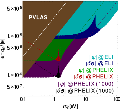
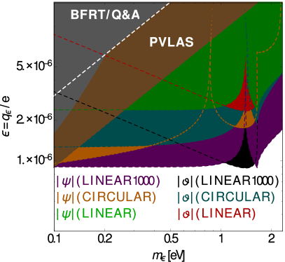
Figure 1: Estimates of constraints for MCPs of mass $m_{\epsilon}$ and relative coupling constant $\epsilon$ derived from the absence of signals in a plausible polarimetric setup assisted by a linearly polarized Gaussian laser pulse. In both panels, the white dashed line correspond to the expression $\xi_{\epsilon}=1$ which is evaluated with the PHELIX parameters. The colored regions in brown and gray are exclusion areas stemming from various experimental collaborations searching for rotation and ellipticity in constant magnetic fields such as BFRT [29], PVLAS [31] and Q $\&$ A [33]. The respective $95\%$ confidence levels needed to recreate the BFRT and Q$\&$A results are summarized in Ref. [13].

As discussed below Eq. (4), the energy scale $1/w_{0}$ associated with the waist size of the pulse $w_{0}$ limits the applicability of our method to the regime $m_{\epsilon}\gg w_{0}^{-1}$ [$w_{0}\approx 2\lambda_{0}\approx(0.12\ \rm eV)^{-1}$ for HIBEF]. For the detection of QED birefringence a detailed analysis of focussing effects has recently been carried out in Ref. [49] based on an expression for the polarization operator which was obtained from the Euler-Heisenberg Lagrangian [see also [41, 42]]. It was shown there that focussing effects could notably improve the signal-to-noise ratio if probe photons which are scattered slightly away from the forward direction are analyzed. Certainly, this fact might be beneficial in the search of MCPs as well. However, we point out that such a study would require to incorporate transverse focusing effects in the polarization tensor. This computation is challenging in the energy regimes considered here. Conversely, at low energies $\omega_{\boldsymbol{k}}\varkappa_{0}\ll m_{\epsilon}^{2}$, the Euler-Heisenberg Lagrangian could be used, but this calculation is beyond the scope of this work.

Next, let us estimate the projected limits resulting from a technically feasible experiment in which the rotation of the polarization plane [see Eq. (13)] and the ellipticity [see Eq. (14)] are probed with an optical laser beam, but none of them is detected. In practice, the absence of these signals provides certain upper limits $\psi_{\mathrm{CL}\%}$, $\delta\vartheta_{\mathrm{CL}\%}$ which are understood within certain confidence levels, frequently corresponding to $2\sigma$. Hereafter, we take $\psi_{\mathrm{CL}\%},\ \delta\vartheta_{\mathrm{CL}\%}\sim 10^{-10}\ \mathrm{rad}$. This choice is in agreement with the experimental accuracies with which both observables can nowadays be measured in the optical regime. Here, the projected sensitivities result from the inequalities $10^{-10}\ \mathrm{rad}>|\psi(\epsilon,m_{\epsilon})|\quad$ and $10^{-10}\ \mathrm{rad}>|\delta\vartheta(\epsilon,m_{\epsilon})|$. Firstly, we consider the nanosecond front-end of the PHELIX laser [71], [$\tau\approx 20\ \rm ns$, $\varkappa_{0}\approx 1.17\ \rm eV$ implying $\Delta\varphi\approx 5\times 10^{6}\pi$, $I_{\mathrm{max}}\approx 10^{16}\ \rm W/cm^{2}$, $\xi\approx 6.4\times 10^{-2}$, $w_{0}\approx 100-150\ \mu\mathrm{m}$] combined with a frequency doubled probe beam [$\omega_{\boldsymbol{k}}=2\varkappa_{0}=2.34\ \rm eV$], having a waist size and an intensity much smaller than the corresponding ones of the strong laser field.

The projected exclusion regions associated with this laser setup are shaded in Fig. 1 in green and red. These should be trustworthy as long as the limits lie much below the curve corresponding to $\xi_{\epsilon}=\epsilon m\xi/m_{\epsilon}=1$, i.e. the white dashed line in the upper left corner. We remark that our potential exclusion bounds are valid whenever the condition $m_{\epsilon}\gg w_{0}^{-1}$ is satisfied. This translates into $m_{\epsilon}\gg 1.3\ \rm meV$. In line with this last aspect, we note that the pulse length associated with PHELIX is much larger than its wave period [$\tau\gg\varkappa_{0}^{-1}$] and, furthermore, satisfies the condition $w_{0}\gg\lambda_{0}$. Therefore, the electromagnetic field produced by this laser system can be treated theoretically as a monochromatic plane wave. It is also worth observing that the square of the intensity parameter associated with the PHELIX beam is much smaller than unity $\xi^{2}\ll 1$ [$\xi_{\epsilon}^{2}\ll 1$ in the relevant parameter space]. Under these circumstances, the observables [see Eqs. (13) and (14)] are dominated by a dependence of the form $\propto\xi^{2}\Delta\varphi$, as can be read off from Eqs. (32) and (33). This fact indicates that–for $\omega_{\boldsymbol{k}}\sim 1\ \rm eV$–large sensitivities can be achieved provided $\Delta\varphi$ compensates for the relative smallness of $\xi$. As we anticipated in Sec. 3.2, this enhancement is particularly large in the vicinity of the threshold mass $m_{1}\approx 1.64\ \rm eV$ because the cross section for photon-photon scattering is maximized nearby the pair creation threshold. Here, the projected bound coming from a search of the induced ellipticity turns out to be $\epsilon<2.8\times 10^{-6}$.

We note that the exclusion plot exhibits a discontinuity at the threshold mass [see discussion below Eq. (34)]. Upper bounds for large masses can be derived when higher order processes–such as the three photon reaction–are taken into account [58, 59]. The effects resulting from this phenomenon are summarized in the right panel of Fig. 1 [orange area]. This outcome as well as the one in darker cyan for the rotation angle were obtained previously by assuming the strong field as a circularly polarized wave and considering a procedure beyond the Born approximation [58, 59]. We note that in the case of circular polarization a slightly more stringent bound of $\epsilon<1.9\times 10^{-6}$ at $m_{1}\approx 1.64\ \rm eV$ results from the induced ellipticity.

Both panels include regions colored in purple and black labeled by PHELIX1000. These excluded areas have been determined by using the PHELIX parameters given above but supposing that the signals gain sensitivity by a factor of $\sim 50$. This could be achieved if a series of plasma mirrors induces $1000$ crossings of the two beams as suggested by Tommasini et al. [48]. This method is feasible for intensities below $\sim 10^{19}\ \rm W/cm^{2}$ and would require a collision angle very close to $\pi$. Besides, the mirrors should exceed the waist size of the pulse in order to avoid diffractive distortions; for further details see [48]. Using the same sensitivity of $\sim 10^{-10}$ as above, the exclusion limit is pushed down to $\epsilon<8.8\times 10^{-7}$ at the threshold mass $m_{1}\approx 1.64\ \rm eV$ [for all projected sensitivities we assume a counter propagating geometry $\varkappa_{+}k_{-}=2\varkappa_{0}\omega_{\boldsymbol{k}}$ and an initial polarization angle $\vartheta_{0}=\pi/4$].

As a last scenario, we consider the envisaged parameters at ELI: $\tau\approx 13\ \rm fs$, $\varkappa_{0}\approx 1.55\ \rm eV$ [$\lambda_{0}=800\ \rm nm$] corresponding to $\Delta\varphi\approx 4\pi$, $I\approx 10^{25}\ \rm W/cm^{2}$, $\xi\approx 1.5\times 10^{3}$. Here, we analyze the results taking the probe beam with doubled frequency $\omega_{\boldsymbol{k}}=2\varkappa_{0}=3.1\ \rm eV$, a waist size and an intensity much smaller than the one of the strong laser field, whereas $\psi_{\mathrm{CL}\%},\ \delta\vartheta_{\mathrm{CL}\%}\sim 10^{-10}\ \mathrm{rad}$. Furthermore, a single-crossing geometry is assumed again. The projected exclusion areas are shaded in the left panel of Fig. 1 in cyan and blue. Since the field of the pulse at ELI is expected to be strongly focused [$w_{0}\sim\lambda_{0}$], the estimates associated with this setup are expected to be reasonable as long as $m_{\epsilon}\gg 0.1\ \rm eV$ and the upper limit of $\epsilon$ lies much above the curves corresponding to $\xi_{\epsilon}=1$ and $\zeta_{\epsilon}^{\nicefrac{{1}}{{3}}}=\xi_{\epsilon}$. [Note that these curves lie far below the region encompassed by the figure.] We observe that, in the ELI scenario, the path of the projected exclusion bounds resembles those established from experiments driven by constant magnetic fields [11, 12, 13].

5 Conclusions

We have studied the prospects that laser-based experiments, designed to detect vacuum birefringence, offer for probing hypothetical degrees of freedom with a tiny fraction of the electron charge. Throughout this investigation, we have indicated that the vacuum of MCPs might induce ellipticity and rotation on the incoming polarization plane, even though the probe photon energy is much below the threshold of electron-positron pair production. In such a scenario, the transmission probability through an analyzer set crossed to the initial polarization direction would not be determined solely by the QED ellipticity but also by the ellipticity and the rotation angle induced by MCPs. We have argued that a slightly modified version of the proposed polarimeter for a x-ray probe would allow for measuring both signals separately. The projected bounds resulting from this analysis will depend on the choice of the wave profile. In contrast to previous studies, the treatment presented here has taken into account the effects resulting from a Gaussian envelop. With the help of contemporary techniques based on plasma mirrors, polarimetric studies driven by an optical laser pulse of moderate intensity [$\sim 10^{16}\ \rm W/cm^{2}$] might allow for excluding MCPs with $\epsilon>9\times 10^{-7}$ and masses $0.1\ \mathrm{eV}\leqslant m_{\epsilon}<1.5\ \mathrm{eV}$, a region which has not been discarded so far by experiments driven by constant magnetic fields and where the best model-independent cosmological limits–resulting from CMB data–are of the same order of magnitude [72].

Acknowledgments

The authors thank A. Di Piazza and S. Bragin for useful comments to the manuscript. S. Villalba-Chávez and C. Müller gratefully acknowledge the funding by the German Research Foundation (DFG) under Grant No. MU 3149/2-1.

References

• [1]
• [2] B. Batell, T. Gherghetta, Phys. Rev. D 73, 045016 (2006).
• [3] F. Brummer, J. Jaeckel and V. V. Khoze, JHEP 0906, 037 (2009).
• [4] F. Brummer, and J. Jaeckel Phys. Lett. B 675, 360 (2009).
• [5] E. Dudas, Y. Mambrini, S. Pokorski and A. Romagnoni, JHEP 1210, 123 (2012).
• [6] M. Goodsell, J. Jaeckel, J. Redondo and A. Ringwald, JHEP 0911, 027 (2009); [arXiv:0909.0515 [hep-ph]].
• [7] P. Langacker, Rev. Mod. Phys.  81, 1199 (2009).
• [8] L. B. Okun, Sov. Phys. JETP 56, 502 (1982); [Zh. Eksp. Teor. Fiz.  83 (1982) 892].
• [9] B. Holdom, Phys. Lett. B 166, 196 (1986).
• [10] B. A Dobrescu and I. Mocioiu, JHEP 005, 0611 (2006).
• [11] H. Gies, J. Jaeckel and A. Ringwald, Phys. Rev. Lett. 97, 140402 (2006); [arXiv:hep-ph/0607118].
• [12] M. Ahlers, H. Gies, J. Jaeckel, J. Redondo and A. Ringwald, Phys. Rev. D. 76, 115005 (2007); [arXiv:0706.2836 [hep-ph]].
• [13] M. Ahlers, H. Gies, J. Jaeckel, J. Redondo, and A. Ringwald, Phys. Rev. D. 77, 095001 (2008); [arXiv:0711.4991 [hep-ph]].
• [14] S. Davidson et al., JHEP 05, 003 (2000).
• [15] E. Masso and J. Redondo, JCAP 0509, 015 (2005).
• [16] E. Masso and J. Redondo, Phys. Rev. Lett. 97, 151802 (2006).
• [17] J. Jaeckel, E. Masso, J. Redondo, A. Ringwald and F. Takahashi, We need lab experiments to look for axion-like particles, arXiv: hep-ph/0605313.
• [18] J.  Jaeckel et al., Phys. Rev. D 75, 013004 (2007).
• [19] K. Ehret et al. [ALPS collaboration], Phys. Lett. B 689, 149 (2010).
• [20] A. S. Chou et al. [GammeV (T-969) Collaboration], Phys. Rev. Lett. 100, 080402 (2008).
• [21] J. H. Steffen and A. Upadhye, Mod. Phys. Lett. A 24, 2053 (2009).
• [22] A. Afanasev et al., Phys. Rev. Lett. 101, 120401 (2008).
• [23] P. Pugnat [OSQAR Collaboration], Phys. Rev. D 78, 092003 (2008).
• [24] C. Robilliard et al., Phys. Rev. Lett. 99, 190403 (2007).
• [25] M.  Fouche et al., Phys. Rev. D. 78, 032013 (2008).
• [26] B. Döbrich, H. Gies, N. Neitz and F. Karbstein, Magnetically amplified tunneling of the 3rd kind as a probe of minicharged particles, Phys. Rev. Lett.  109, 131802 (2012); [arXiv:1203.2533 [hep-ph]].
• [27] J. Jaeckel, Phys. Rev. Lett. 103, 080402 (2009).
• [28] J. Jaeckel and S. Roy, Phys. Rev. D 82, 125020 (2010).
• [29] R. Cameron et al., Phys. Rev. D 47, 3707 (1993).
• [30] E. Zavattini et al. [PVLAS Collaboration], Phys. Rev. D 77, 032006 (2008).
• [31] F. Della Valle et al. [PVLAS Collaboration], Phys. Rev. D 90, 092003 (2014).
• [32] A. Cadéne et al., Eur. Phys. J. D 68, 16 (2014).
• [33] S. J. Chen, H. H. Mei and W. T. Ni, Mod. Phys. Lett. A 22, 2815 (2007).
• [34] J. Jaeckel and A. Ringwald, Ann. Rev. Nucl. Part. Sci. 60, 405 (2010).
• [35] A. Ringwald, Phys. Dark Univ. 1, 116 (2012); [arXiv:1210.5081 [hep-ph]].
• [36] J. L. Hewett et al., Fundamental Physics at the Intensity Frontier, The Proceedings of the 2011 workshop on Fundamental Physics at the Intensity Frontier; arXiv:1205.2671 [hep-ex].
• [37] R. Essig et al., Working Group Report: New Light Weakly Coupled Particles, arXiv:1311.0029 [hep-ph].
• [38] A. Di Piazza, C.  Müller, K. Z.   Hatsagortsyan and C. H. Keitel, Rev. Mod. Phys. 84, 1177 (2012); [arXiv:1111.3886 [hep-ph]].
• [39] See: http://www.extreme-light-infrastructure.eu
• [40] See: http://www.xcels.iapras.ru/
• [41] T. Heinzl, B. Leifeld, K. U. Amthor, H. Schwoerer, R. Sauerbrey, and A.  Wipf, Opt. Comm. 267, 318 (2006).
• [42] A. Di Piazza et al., Phys. Rev. Lett. 97, 083603 (2006).
• [43] V. Dinu, T. Heinzl, A. Ilderton, M. Marklund, and G.  Torgrimsson, Phys. Rev. D 89, 125003 (2014); [arXiv:1312.6419 [hep-ph]].
• [44] V. Dinu, T. Heinzl, A. Ilderton, M. Marklund, and G.  Torgrimsson, Phys. Rev. D 90, 045025 (2014); [arXiv:1405.7291 [hep-ph]].
• [45] B. King, and T. Heinzl, High Power Laser Science and Engineering 4, e5 (2016); arXiv:1510.08456 [hep-ph].
• [46] See: http://www.hzdr.de/db/Cms?pNid=427$\&$pOid=35325
• [47] H. P. Schlenvoigt, T. Heinzl, U. Schramm, T. E Cowan, and R.  Sauerbrey, Phys. Scr. 91, 023010 (2016).
• [48] D. Tommasini, A. Ferrando, H. Michinel and M. Seco, JHEP 0911, 043 (2009); [arXiv:0909.4663 [hep-ph]].
• [49] F. Karbstein, H. Gies, M. Reuter and M. Zepf, Phys. Rev. D 92, 071301 (2015); [arXiv:1507.01084 [hep-ph]].
• [50] B. King and N. Elkina, “Vacuum birefringence in high-energy laser-electron collisions,” arXiv:1603.06946 [hep-ph].
• [51] Y. Nakamiya, K. Homma, T. Moritaka and K. Seto,“Probing vacuum birefringence under a high-intensity laser field with gamma-ray polarimetry at the GeV scale,” arXiv:1512.00636 [hep-ph].
• [52] J. T. Mendonça, Eurphys. Lett. 79, 21001 (2007).
• [53] H. Gies, Eur. Phys. J. D 55, 311 (2009); [arXiv:0812.0668 [hep-ph]].
• [54] B. Döbrich and H. Gies, JHEP 1010, 022 (2010); [arXiv:1006.5579 [hep-ph]].
• [55] S. Villalba-Chávez and A. Di Piazza, JHEP 1311, 136 (2013); [arXiv:1307.7935 [hep-ph]].
• [56] S. Villalba-Chávez, Nucl. Phys. B 881, 1 (2014); [arXiv:1308.4033 [hep-ph]].
• [57] S. Villalba-Chávez and C. Müller, Annals Phys. 339, 460 (2013); [arXiv:1306.6456 [hep-ph]].
• [58] S. Villalba-Chávez and C. Müller, JHEP 1506, 177 (2015); [arXiv:1412.4678 [hep-ph]].
• [59] S. Villalba-Chávez and C. Müller, JHEP 1602, 027 (2016); [arXiv:1510.00222 [hep-ph]].
• [60] E. Gabrielli, L. Marzola, E. Milotti and H. Veermäe, arXiv:1604.00393 [hep-ph].
• [61] V. N.  Baĭer, A. I.  Mil’shteĭn and V. M.  Strakhovenko, Zh. Eksp. Teo. Fiz. 69, 1893 (1975); [Sov. Phys. JETP 42, 961 (1976)].
• [62] W. Becker and H. Mitter, J.  Phys.  A  8, 1638 (1975).
• [63] S. Meuren, C. H. Keitel, and A. Di Piazza, Phys. Rev. D 88, 013007 (2013); [arXiv:1304.7672 [hep-ph]].
• [64] S. Meuren, K. Z. Hatsagortsyan, C. H. Keitel, and A. Di Piazza, Phys. Rev. D 91, 013009 (2015); [arXiv:1406.7235 [hep-ph]].
• [65] S. Villalba-Chavez and C. Müller. Phys. Lett. B, 718, 992, 2013; arXiv:1208.3595 [hep-ph].
• [66] M. Born and E. Wolf, Principles of optics, Pergamon Press, (1999).
• [67] B. Marx et al., Opt. Commun. 284, 915 (2011).
• [68] B. Marx et al., Phys. Rev. Lett. 110, 254801 (2013).
• [69] H. P. Schlenvoigt, private communication.
• [70] F. W. J. Olver, D. W. Lozier, R. F. Boisvert, and C. W. Clark, NIST Handbook of Mathematical Functions, Cambridge University Press, England, (2010).
• [71] See: https://www.gsi.de/en/work/research/appamml/plasma_physicsphelix/phelix.htm
• [72] A. Melchiorri, A. D. Palosa, and A. Strumia, Phys. Lett. B 650, 416 (2007).