Time dependent electromagnetic fields and 4-dimensional Stokes’ theorem

Abstract

Stokes’ theorem is central to many aspects of physics – electromagnetism, the Aharonov-Bohm effect, and Wilson loops to name a few. However, the pedagogical examples and research work almost exclusively focus on situations where the fields are time-independent so that one need only deal with purely spatial line integrals (e.g. $\oint{\bf A}\cdot d{\bf x}$) and purely spatial area integrals (e.g. $\int(\nabla\times{\bf A})\cdot d{\bf a}=\int{\bf B}\cdot d{\bf a}$). Here we address this gap by giving some explicit examples of how Stokes’ theorem plays out with time-dependent fields in a full 4-dimensional spacetime context. We also discuss some unusual features of Stokes’ theorem with time-dependent fields related to gauge transformations and non-simply connected topology.

I Stokes’ theorem in 3 and 4 dimensions

I.1 3D Stokes’ theorem

Stokes’ theorem is used in many areas of physics, particularly in electricity and magnetism where it gives a connection between the electromagnetic potentials (i.e. $\phi$ and ${\bf A}$) and the fields (i.e. ${\bf E}$ and ${\bf B}$). Through Stokes’ theorem, the connection between the line integral of the 3-vector potential, ${\bf A}$, and the area integral of the magnetic field, ${\bf B}$, is

$$\oint_{C}{\bf A}\cdot d{\bf x}=\int_{S}(\nabla\times{\bf A})\cdot d{\bf a}=\int_{S}{\bf B}\cdot d{\bf a}~{},$$ (1)

The subscripts $C$ and $S$ on the integrals indicate line and surface integrals respectively. The closed contour $C$ is spanned by an infinite number of possible surfaces $S$. The contour has a direction of traversal which is determined by the direction of $d{\bf x}$, and this determines the direction of the vector area, $d{\bf a}$, of the surface, $S$, via the right-hand-rule (wrap the fingers of the right hand in the direction that the contour is traversed and the thumb points in the direction of the vector area). This issue of the directionality of the area in Stokes’ theorem will be important (but less familiar) when we move from a purely spatial area to a spacetime area. In the rest of the paper we will drop the subscripts $C$ and $S$ if there is no confusion as to whether the integral is a line or surface integral.

The usual pedagogical examples of (1) involve time-independent 3-vector potentials and magnetic fields. One common example in cylindrical coordinates is a solenoid of radius $R$, with the axis of the solenoid and the magnetic field along the $z$-axis. The magnetic field for this setup is

$${\bf B}=B_{0}{\hat{\bf z}}~{}~{}{\rm for}~{}~{}\rho<R~{}~{}~{}~{}~{}{\rm and}~{}~{}~{}~{}~{}{\bf B}={\bf 0}~{}~{}{\rm for}~{}~{}\rho\geq R~{},$$ (2)

where $B_{0}$ is the constant value of the magnetic field. The vector potential has the following form

$${\bf A}=\frac{B_{0}\rho}{2}{\hat{\boldsymbol{\varphi}}}~{}~{}{\rm for}~{}~{}\rho<R~{}~{}~{}~{}{\rm and}~{}~{}~{}~{}~{}{\bf A}=\frac{B_{0}R^{2}}{2\rho}{\hat{\boldsymbol{\varphi}}}~{}~{}{\rm for}~{}~{}\rho\geq R~{}.$$ (3)

For a contour that is a circle of radius $\rho>R$ which goes around the solenoid, the area integral in (1) yields $\int{\bf B}\cdot d{\bf a}=B_{0}\pi R^{2}$. For the line integral one similarly finds $\oint{\bf A}\cdot d{\bf x}=B_{0}\pi R^{2}$. Thus, for this setup, Stokes’ theorem works out to give

$$\oint{\bf A}\cdot d{\bf x}=B_{0}\pi R^{2}=\int{\bf B}\cdot d{\bf a}~{}.$$ (4)

The above example is also the heart of the time-independent Aharonov-Bohm effect AB where one performs the usual quantum mechanical two-slit experiment but with an infinite solenoid, described by the above ${\bf B}$ and ${\bf A}$, inserted between the slits of the experiment. For example, say one sends electrons at a two-slit set up. The electrons will form an interference pattern on a screen placed down stream from the two slits due to the quantum mechanical wave nature of the electrons. In this simple two-slit experiment the interference occurs due to the phase difference of the wavefunction coming from the two different slits, and this comes from the path length difference from each slit to whatever point on the down stream screen one is interested in. The Aharonov-Bohm effect comes from placing an infinite solenoid between the slits. Classically one does not expect any change since, classically, charged particles only respond to the magnetic field, via $\frac{{\bf v}}{c}\times{\bf B}$, not the vector potential. However quantum mechanically, due to minimal coupling, the electrons will pick up a phase, $\frac{e}{\hbar c}\int_{\gamma}{\bf A}\cdot d{\bf x}$, when traveling along a contour $\gamma$. Now for some particular point on the screen there will be two paths leading from each slit to that point – call these two paths $\gamma_{1}$ and $\gamma_{2}$. Now in addition to the phase difference due to the path length difference there will be an additional phase difference coming from the line integrals of the vector potential namely $\frac{e}{\hbar c}\int_{\gamma_{1}}{\bf A}\cdot d{\bf x}-\frac{e}{\hbar}\int_{\gamma_{2}}{\bf A}\cdot d{\bf x}=\frac{e}{\hbar c}\oint{\bf A}\cdot d{\bf x}=\frac{e}{\hbar c}\int{\bf B}\cdot d{\bf a}$. Thus one gets a phase shift of the standard interference pattern of the two-slit experiment, which is given by $\frac{e}{\hbar c}\oint{\bf A}\cdot d{\bf x}=\frac{e}{\hbar c}\int{\bf B}\cdot d{\bf a}$. This is the heart of the time-independent Aharonov-Bohm experiment – that one gets a phase shift in the interference pattern of the two-slit experiment despite the fact that the electrons move in a region which if ${\bf B}$ field free, but where the vector potential, ${\bf A}$, is non-zero. A fuller and more detailed account of the Aharonov-Bohm effect can be found in section 3.4 of reference ryder . Due to the close connection between Stokes’ theorem and the Aharonov-Bohm effect we have in mind that the contours and surfaces discussed in this paper in connection with Stokes’ theorem should be those associated with the paths and surfaces of particles in an Aharonov-Bohm experiment.

The magnetic field in (2) can also be obtained from a vector potential of the following form

$${\bf A}^{\prime}=\left[\frac{B_{0}\rho}{2}-\frac{B_{0}R^{2}}{2\rho}\right]{\hat{\boldsymbol{\varphi}}}~{}~{}{\rm for}~{}~{}\rho<R~{}~{}~{}~{}{\rm and}~{}~{}~{}~{}~{}{\bf A}^{\prime}={\bf 0}~{}~{}{\rm for}~{}~{}\rho\geq R~{}.$$ (5)

This form of the vector potential is related to the original form given in (3) by the following gauge transformation

$${\bf A}^{\prime}\rightarrow{\bf A}+{\bf\nabla}\chi~{}~{}~{}{\rm with}~{}~{}~{}\chi=-\frac{B_{0}R^{2}\varphi}{2}$$ (6)

Note that the gauge function, $\chi$ is non-single valued and ${\bf A}^{\prime}$, for $\rho<R$, has a $\frac{1}{\rho}$ singularity. These features (singular vector potential and non-single valued gauge function) indicate that while the ${\bf B}$ field produced by the two different vector potentials in (3) and (5) is the same the physical situation is different – for the vector potential (5) one has the original solenoid of radius $R$ plus an idealized, infinitely thin solenoid placed along the symmetry axis with a current flowing in the opposite direction of the original solenoid. We will show shortly how to deal with this singularity in ${\bf A}^{\prime}$. One might naively conclude that Stokes’ theorem fails in this new gauge. The area integral, $\int{\bf B}\cdot d{\bf a}=B_{0}\pi R^{2}$, is still the same since the ${\bf B}$ field is still given by (2). However, for the circular contour with radius $\rho>R$, apparently $\oint{\bf A}^{\prime}\cdot d{\bf x}=0$ since ${\bf A}^{\prime}=0$. The problem is the singularity at $\rho=0$ in ${\bf A}^{\prime}$ inside the solenoid. Due to this “puncture”, the space is said to have a non-simply connected topology. One can not span the simple circle contour with a surface that includes $\rho=0$ since this point is no longer part of the space. To deal with this “puncture” at $\rho=0$, we need to deform the simple circle contour into the more complex contour in Fig. (1), which avoids $\rho=0$. The outer circular contour gives zero ($\int_{outer}{\bf A}^{\prime}\cdot d{\bf x}=0$) since ${\bf A}^{\prime}=0$ for $\rho>R$. The line integrals for the two radial segments cancel. The only non-zero contribution is from the inner circular contour with an infinitesimal radius $\epsilon\ll R$. Since the inner contour is traversed in the opposite direction from the outer contour, the inner line integral has a negative sign relative to the outer line integral. Putting it all together one finds that for the contour in Fig. (1).

$$\oint{\bf A}^{\prime}\cdot d{\bf x}=\int_{inner}{\bf A}^{\prime}\cdot d{\bf x}=-\int_{0}^{2\pi}\left[\frac{B_{0}\epsilon}{2}-\frac{B_{0}R^{2}}{2\epsilon}\right]\epsilon d\varphi=B_{0}\pi R^{2}-B_{0}\pi\epsilon^{2}\rightarrow B_{0}\pi R^{2}~{}.$$ (7)

In the last step we have let $\epsilon\rightarrow 0$. This removes the singularity in ${\bf A}^{\prime}$ at $\rho=0$, and we find $\oint{\bf A}^{\prime}\cdot d{\bf x}=\int{\bf B}\cdot d{\bf a}$ for the contour in Fig. (1), thus satisfying Stokes’ theorem.

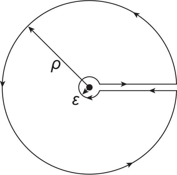
Figure 1: The modified contour for the gauge potential from (5) The inner circle has a radius $\epsilon\ll R$ and the outer circle a radius $\rho>R$.

I.2 4D Stokes’ theorem

The discussion of the previous subsection was in terms of the 3-vector potential. Since ${\bf A}$ is part of the 4-vector $A^{\mu}=(\phi,{\bf A})$, we can generalize the first expression in equation (1) as

$$\oint{\bf A}\cdot d{\bf x}\rightarrow\oint A_{\mu}dx^{\mu}=-\oint\phi~{}cdt+\oint{\bf A}\cdot d{\bf x}~{},$$ (8)

This generalization was noted already in AB and is discussed in more detail in references macdougall ; ryder . Equation (8) involves both a spatial line integral as well as a time integral, thus making it ideal for time-dependent situations. In the section below we will make this last statement more concrete by looking at the specific example of a time-dependent solenoid with various contours. It should be noted that throughout the paper we use the $(-+++)$ metric signature rather than the $(+---)$ signature used in references AB ; macdougall ; ryder . Next, the right hand side of (1), which involves the magnetic field, can be generalized as macdougall ; ryder

$$\int{\bf B}\cdot d{\bf a}\rightarrow\int{\bf E}\cdot d{\bf x}~{}cdt+\int{\bf B}\cdot d{\bf a}=\frac{1}{2}\int F_{\mu\nu}d\sigma^{\mu\nu}~{},$$ (9)

where in the last expression $F_{\mu\nu}=\partial_{\mu}A_{\nu}-\partial_{\nu}A_{\mu}$ is the Maxwell field strength tensor and $d\sigma^{\mu\nu}$ is an infinitesimal spacetime area. The signs of the area integrals of the fields of the intermediate expression in (9) can be checked using the expression for the contour integrals of the potentials in (8) in the following way: dropping the scalar potential part of (8) and the electric area integral of (9) one recovers the usual result $\oint{\bf A}\cdot d{\bf x}=\int{\bf B}\cdot d{\bf a}$; in turn dropping the 3-vector potential line integral of (8) and magnetic field area integral part of (9), one recovers the standard relationship $\phi=-\int{\bf E}\cdot d{\bf x}$ (inside the time integration).

In the next section, we apply Stokes’ theorem to an explicit example which involves time-dependent fields and potentials and which uses the full four-vector potential, $A^{\mu}=(\phi,{\bf A})$.

II The infinite, time-dependent solenoid

In this section we study the case of an infinite solenoid of radius $R$ with a time-dependent magnetic flux. We first consider a spacetime loop which does not enclose the solenoid. For concreteness and simplicity, we take the time dependence to be linear so that the 4-vector potential takes the form

$$A^{\mu}=\left(0,0,\frac{B_{0}t\rho}{2}{\hat{\boldsymbol{\varphi}}},0\right)~{}~{}{\rm for}~{}~{}\rho<R~{}~{}~{}{\rm and}~{}~{}~{}A^{\mu}=\left(0,0,\frac{B_{0}tR^{2}}{2\rho}{\hat{\boldsymbol{\varphi}}},0\right)~{}~{}{\rm for}~{}~{}\rho\geq R~{}.$$ (10)

The scalar potential is zero (i.e. $\phi=0$). This is similar to the expression given in (3) but with $B_{0}\rightarrow B_{0}t$. Note that in (10) $B_{0}$ is a rate of magnetic field strength change, while in (3) $B_{0}$ is just the magnetic field strength. The magnetic field connected with the vector potential in (10) is

$${\bf B}=B_{0}t{\hat{\bf z}}~{}~{}{\rm for}~{}~{}\rho<R~{}~{}~{}~{}{\rm and}~{}~{}~{}~{}~{}{\bf B}={\bf 0}~{}~{}{\rm for}~{}~{}\rho\geq R~{},$$ (11)

and the electric field connected with (10) is

$${\bf E}=-\frac{B_{0}\rho}{2c}{\hat{\boldsymbol{\varphi}}}~{}~{}{\rm for}~{}~{}\rho<R~{}~{}~{}~{}{\rm and}~{}~{}~{}~{}~{}{\bf E}=-\frac{B_{0}R^{2}}{2\rho c}{\hat{\boldsymbol{\varphi}}}~{}~{}{\rm for}~{}~{}\rho\geq R~{}.$$ (12)

The linear time dependence of the magnetic flux yields the above simple fields – ${\bf A},{\bf B}$ and ${\bf E}$. The potential and fields in (10) (11) and (12) correspond to those given in griffiths if the large time limit is taken. In griffiths the linear increasing flux is turned on at $t=0$ whereas the potentials and fields above are linearly increasing for all time, but as $t$ becomes large the results of griffiths yield those given above after units conversion.

The 3-vector potential in (10) can be “redistributed” to form a new scalar and 3-vector potential, which gives the same electric and magnetic fields. The new 4-vector potential is

$${A^{\prime}}^{\mu} = \left(\phi^{\prime},{\bf A}^{\prime}\right)=\left(\frac{B_{0}R^{2}\varphi}{2c},0,\left[\frac{B_{0}t\rho}{2}-\frac{B_{0}R^{2}t}{2\rho}\right]{\hat{\boldsymbol{\varphi}}},0\right)~{}~{}{\rm for}~{}~{}\rho<R$$ (13)

$$~{}~{}~{}~{}{\rm and}~{}~{}~{}~{}~{}$$

$${A^{\prime}}^{\mu} = \left(\phi^{\prime},{\bf A}^{\prime}\right)=\left(\frac{B_{0}R^{2}\varphi}{2c},0,0,0\right)~{}~{}{\rm for}~{}~{}\rho\geq R~{},$$ (14)

The two forms of the potentials for the time-dependent solenoid are related by a gauge transformation given by

$${A^{\prime}}^{\mu}\rightarrow A^{\mu}+\partial^{\mu}\chi~{}~{}~{}{\rm with}~{}~{}~{}\chi=-\frac{B_{0}R^{2}\varphi t}{2}$$ (15)

As in the previous time-independent case given in (5) (6), ${\bf A}^{\prime}$ has a $\frac{1}{\rho}$ singularity and the gauge function, $\chi$, is non-single valued.

We begin by first evaluating $\oint A_{\mu}dx^{\mu}$ for these two gauges as given in equations (10) and (13) (14), on the closed spacetime path shown in figure (2).

II.1 Spacetime loop integral for the 4-vector potential from (10)

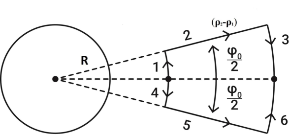
Figure 2: Closed loop path outside a solenoid with a time-changing magnetic flux.

The evaluation of the loop integral $\oint A_{\mu}dx^{\mu}$ for the potential in (10) is split into 6 segments, as shown in Fig. (2). Since in the end we want to connect our discussion of the time-dependent Stokes’ theorem with the time-dependent Aharonov-Bohm effect singleton , we will take our paths to be those traversed by a particle and thus the path lengths will be parameterized in terms of the particle’s velocity. We will take the linear speed of the particle to be the same along every path. In general Stokes’ theorem could apply to paths which are not physically realizable paths for a particle. For example, even for the time-dependent case one could take a circular path around the solenoid at one instant in time. In this case one would just get $\oint{\bf A}\cdot d{\bf x}=\int{\bf B}\cdot d{\bf a}$ but the circular path would not be one that a real particle could travel. In addition, one would not touch on the time-dependent nature of this case which, is one of the central points of this article.

Stokes’ theorem with time-independent fields has closed spatial loops when evaluating $\oint{\bf A}\cdot d{\bf x}$. Similarly, the time-dependent case has closed spacetime loops. To create a closed spacetime loop we consider two particles which begin at the same spacetime point, move apart and then come back together. We then time reverse the path of one of the particles and add this to the result of the path of the other particle. This is also the procedure for the Aharonov-Bohm effect with time-independent fields. The paths of the two moving particles are shown, with paths 1, 2 and 3 for one particle and paths 4, 5 and 6 for the other particle. The arrows indicate the real directions of travel of each particle, starting from the middle of the inner arc at radius $\rho_{1}$ and ending at the middle of the outer arc at radius $\rho_{2}$ . To obtain a closed spacetime path we apply the time reversal operator, $T[...]$, to the results of the line integrals for paths 4, 5 and 6. The operation of $T[...]$ takes $t\rightarrow-t$. The results of applying $T[...]$ to other physical quantities can be found in section 6.10 of reference. jackson The oddness of ${\bf A}$ under time reversal (i.e. $T[{\bf A}]=-{\bf A}$) and the evenness of ${\bf x}$ under time reversal (i.e. $T[{\bf x}]={\bf x}$) implies that $T[\int{\bf A}\cdot d{\bf x}]=-\int{\bf A}\cdot d{\bf x}$. Thus the operation of $T[...]$ in segments 4, 5 and 6 has the effect of multiplying the results of these line integrals by $-1$. To get the closed spacetime loop we add the time reversed paths 4, 5 and 6 to the results from paths 1, 2 and 3. Paths 1, 3, 4 and 6 cover an angle of $\varphi_{0}/2$, with 1 and 3 going between $0$ and $\varphi_{0}/2$, and with 4 and 6 going between $0$ and $-\varphi_{0}/2$. The linear speed of the particles is taken to be constant throughout so that the angular speed along the inner paths, 1 and 4, is larger than the angular speed along the outer paths, 3 and 6. The detailed definitions and calculations for each segment are given in Appendix I. Using these results we find that the closed spacetime loop is

$$\oint A_{\mu}dx^{\mu} = \left(\int_{1}+\int_{2}+\int_{3}+T\left[\int_{6}+\int_{5}+\int_{4}\right]\right){\bf A}\cdot d{\bf x}$$ (16)

$$= -\frac{B_{0}R^{2}\varphi_{0}^{2}}{8\omega}\left[\frac{\rho_{2}}{\rho_{1}}+\frac{4(\rho_{2}-\rho_{1})}{\rho_{1}\varphi_{0}}+1\right]~{}.$$

In (16) $\omega$ is the angular speed at which paths 1 and 4 from Fig. (2) are traversed; $\rho_{1}$ is the distance from the center of the solenoid to the inner paths 1 or 4; $\rho_{2}$ is the distance from the center of the solenoid to the outer paths 3 and 6. It is important to note for later that, when viewed from above, the direction of traversal of the closed loop is clockwise.

II.2 Spacetime loop integral for the 4-vector potential from (13) and (14)

The evaluation of the loop integral for the 4-potential in (13) now just involves the scalar potential $\oint A_{\mu}dx^{\mu}\rightarrow-\oint\phi^{\prime}cdt$ since ${\bf A}^{\prime}=0$ outside the solenoid. The details of the calculation for the 6 segments can be found in Appendix II. Collecting together the results for the time-reversed paths 4, 5, and 6 (which, as in the previous case, changes the sign for these integrals as given in Appendix II) and adding these to the results from paths 1, 2 and 3 gives the closed spacetime loop result for the potential in this gauge as

$$\oint A_{\mu}^{\prime}dx^{\mu} = -\oint\phi^{\prime}cdt=-\left(\int_{1}+\int_{2}+\int_{3}+T\left[\int_{4}+\int_{5}+\int_{6}\right]\right)\phi^{\prime}cdt$$ (17)

$$= -\frac{B_{0}R^{2}\varphi_{0}^{2}}{8\omega}\left[\frac{\rho_{2}}{\rho_{1}}+\frac{4(\rho_{2}-\rho_{1})}{\rho_{1}\varphi_{0}}+1\right]~{}.$$

Comparing (16) with (17) we see that the two different gauges give the same result for $\oint A_{\mu}dx^{\mu}$, as is expected for this gauge invariant quantity. We next calculate the spacetime area integral of the fields i.e. $\frac{1}{2}\int F_{\mu\nu}d\sigma^{\mu\nu}=\int{\bf E}\cdot d{\bf x}~{}cdt+\int{\bf B}\cdot d{\bf a}$.

II.3 Spacetime area integral for the fields from (11) and (12)

The evaluation of the spacetime area integral $\frac{1}{2}\int F_{\mu\nu}d\sigma^{\mu\nu}$, for the fields in (11) and (12) on the spacetime area implied by Fig. (2), reduces to $\int{\bf E}\cdot d{\bf x}cdt$ since ${\bf B}=0$ outside the solenoid. The detailed calculations for $\int{\bf E}\cdot d{\bf x}cdt$ are given in Appendix III.

We need to combine the results for the spacetime areas associated with the segments 1, 2, and 3 with the time reversed spacetime areas associated with the time-reverse segments for 4, 5 and 6. From jackson , ${\bf E}$ and ${\bf x}$ are even under time reversal (i.e. do not change sign) whereas $t$ is odd (i.e. changes sign). Thus applying $T$ to $\int{\bf E}\cdot d{\bf x}~{}cdt$ changes the sign $T[\int{\bf E}\cdot d{\bf x}~{}cdt]=-\int{\bf E}\cdot d{\bf x}~{}cdt$. This means that the time-reversed spacetime areas associated with segments 4, 5, and 6 are equivalent to the spacetime areas associated with segments 1, 2, and 3. With all this in mind the total spacetime area integral is

$$\int{\bf E}\cdot d{\bf x}~{}cdt = \left(\int_{1}+\int_{2}+\int_{3}+T\left[\int_{6}+\int_{5}+\int_{4}\right]\right){\bf E}\cdot d{\bf x}~{}cdt$$ (18)

$$= -\frac{B_{0}R^{2}\varphi_{0}^{2}}{8\omega}\left[\frac{\rho_{2}}{\rho_{1}}+\frac{4(\rho_{2}-\rho_{1})}{\rho_{1}\varphi_{0}}+1\right]$$

We see that this result agrees with the spacetime line integral of the 4-vector potential from (16) or (17). Thus we find that, for this case, the time-dependent 4D version of Stokes’ theorem is satisfied. In the next subsection we examine the case in which the path encloses the solenoid and therefore the spacetime area has a magnetic field contribution.

II.4 4D Stokes’ Theorem for a path enclosing the solenoid

We now consider a closed spacetime loop that encloses the solenoid as shown in Fig. (3). We will use the the results of the preceding subsections and the appendices to perform the calculations. To enclose the solenoid with a spacetime path we eliminate paths 2, 3, 5 and 6 and then extend paths 1 and 4 around to form a closed loop.

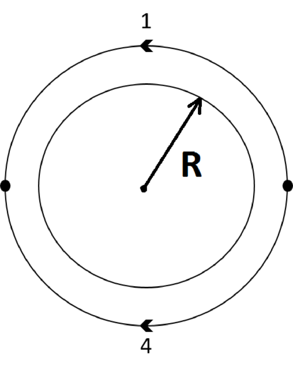
Figure 3: Closed loop path that encloses the solenoid with the time-changing magnetic flux. This closed loop is obtained from the loop in figure (2) by discarding paths 2, 3, 5 and 6 and by extending paths 1 and 4 using $\varphi_{0}=2\pi$.

For the form of the 4-vector potential given in (10), the closed spacetime loop integral, $\oint A_{\mu}dx^{\mu}$, can be obtained using the line integrals of paths 1 and 4 (given by equations (34) and (37) respectively) with $\varphi_{0}=2\pi$

$$\int_{1}{\bf A}\cdot d{\bf x}=\frac{B_{0}R^{2}\pi^{2}}{4\omega}~{}~{}~{}{\rm and}~{}~{}~{}\int_{4}{\bf A}\cdot d{\bf x}=-\frac{B_{0}R^{2}\pi^{2}}{4\omega}~{}.$$ (19)

From (19), one can obtain

$$\oint A_{\mu}dx^{\mu}=+\left(\int_{1}{\bf A}\cdot d{\bf x}+T\int_{4}{\bf A}\cdot d{\bf x}\right)=\frac{B_{0}R^{2}\pi^{2}}{2\omega}~{}.$$ (20)

For this gauge $\oint A_{\mu}dx^{\mu}=-\oint\phi~{}cdt+\oint{\bf A}\cdot d{\bf x}\rightarrow\oint{\bf A}\cdot d{\bf x}$ so only the 3-vector potential contributes. Also $\oint{\bf A}\cdot d{\bf x}=\int_{1}{\bf A}\cdot d{\bf x}-\int_{4}{\bf A}\cdot d{\bf x}$ since the direction of path 4 must be time-reversed to obtain a closed spacetime loop. It is worth noting that, when viewed from above, the path closes in a counterclockwise sense. This is the reverse of the closed path in Fig. (2). This will have important consequences when we discuss the “direction” of the spacetime area associated with the spacetime contours.

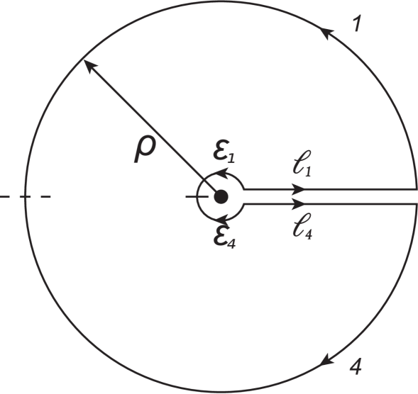
Figure 4: The spacetime loop for the case when the 4-vector potentials are given by (13) and (14). The singularity at $\rho=0$ is excised by the small loop of radius $\epsilon\ll R$. The initial direction of integration of the different paths are shown. To get a closed spacetime loop we time reverse path 4, path $l_{4}$ and path $\epsilon_{1}$.

Next we examine the form of the 4-vector potential given in (13) and (14), obtained from the form of the 4-vector potential given in (10) by the gauge transformation (15). Due to the $\frac{1}{\rho}$ singularity for the $\rho<R$ 4-vector potential (see equation (13)) the “puncture” at $\rho=0$ needs to be removed using a contour similar to the one used in time-independent case (see Fig. (1)). The contour that we use now is shown in Fig. (4), with arrows indicating the direction of travel prior to time reversal of the paths 4, $l_{4}$ and $\epsilon_{1}$. We have contributions from the scalar potential only from paths 1 and 4 on the outer loop. The results from paths 1 and 4 (given by (40) and (43) respectively) with $\varphi_{0}=2\pi$ are

$$\int_{1}\phi^{\prime}cdt=\frac{B_{0}R^{2}\pi^{2}}{4\omega}~{}~{}~{}~{}~{}{\rm and}~{}~{}~{}~{}~{}\int_{4}\phi^{\prime}cdt=-\frac{B_{0}R^{2}\pi^{2}}{4\omega}~{}.$$ (21)

Next we need to take into account the small interior circular path which we take to be of radius $\epsilon\ll R$. Since $\phi^{\prime}=\frac{B_{0}R^{2}\varphi}{2c}$ does not depend on $\rho$, the results for the interior paths will be the same as those in (21) giving

$$\int_{\epsilon_{1}}\phi^{\prime}cdt=\frac{B_{0}R^{2}\pi^{2}}{4\omega}~{}~{}~{}~{}~{}{\rm and}~{}~{}~{}~{}~{}\int_{\epsilon_{4}}\phi^{\prime}cdt=-\frac{B_{0}R^{2}\pi^{2}}{4\omega}~{}.$$ (22)

The subscripts $\epsilon_{1},\epsilon_{4}$ on the integrals above indicate that these are the interior half circle paths of radius $\epsilon\ll R$ corresponding to the outer paths 1 and 4 respectively. We have assumed the traversal of the inner circle is at the same angular velocity, $\omega$, as the outer circle. We will see below that this is the only value for the angular velocity that is able to excise the singularity.

At this point we calculate the scalar potential contribution to $\oint A^{\prime}_{\mu}dx^{\mu}$. From (21) (22), we get

$$\oint\phi^{\prime}cdt = \int_{1}\phi^{\prime}cdt+\int_{\epsilon_{4}}\phi^{\prime}cdt+\int_{l_{1}}\phi^{\prime}cdt+T\left[\int_{4}\phi^{\prime}cdt+\int_{\epsilon_{1}}\phi^{\prime}cdt+\int_{l_{4}}\phi^{\prime}cdt\right]$$ (23)

$$= \frac{B_{0}R^{2}\pi^{2}}{4\omega}-\frac{B_{0}R^{2}\pi^{2}}{4\omega}+\int_{l_{1}}\phi^{\prime}cdt+\frac{B_{0}R^{2}\pi^{2}}{4\omega}-\frac{B_{0}R^{2}\pi^{2}}{4\omega}-\int_{l_{4}}\phi^{\prime}cdt=0$$

Although we did not explicitly calculate $\int_{l_{1}}\phi^{\prime}cdt$ and $\int_{l_{4}}\phi^{\prime}cdt$, it is clear that they are the same in magnitude and cancel after we apply time reversal.

The only non-zero and uncanceled contribution to $\oint A^{\prime}_{\mu}dx^{\mu}$ comes from the interior 3-vector part of (13). The $-\frac{B_{0}R^{2}t}{2\rho}{\hat{\boldsymbol{\varphi}}}$ piece gives the same result as (19) since the extra negative in this part of the 3-potential is balanced by the fact that the inner circular path is traversed in the opposite direction as the outer circle after time reversal. So we have

$$\int_{\epsilon_{1}}{\bf A}^{\prime}\cdot d{\bf x}=\frac{B_{0}R^{2}\pi^{2}}{4\omega}-\frac{B_{0}\epsilon^{2}\pi^{2}}{4\omega}~{}~{}~{}{\rm and}~{}~{}~{}\int_{\epsilon_{4}}{\bf A}^{\prime}\cdot d{\bf x}=-\frac{B_{0}R^{2}\pi^{2}}{4\omega}+\frac{B_{0}\epsilon^{2}\pi^{2}}{4\omega}~{}.$$ (24)

There is an additional contribution from the $\frac{B_{0}\rho t}{2}{\hat{\boldsymbol{\varphi}}}$ term in the 3-potential relative to (19), but in the limit $\epsilon\rightarrow 0$ this additional contribution is zero. From (24), one can obtain

$$\oint A^{\prime}_{\mu}dx^{\mu}=+\left(\int_{\epsilon_{1}}{\bf A}^{\prime}\cdot d{\bf x}+T\int_{\epsilon_{4}}{\bf A}^{\prime}\cdot d{\bf x}\right)=\frac{B_{0}R^{2}\pi^{2}}{2\omega}-\frac{B_{0}\epsilon^{2}\pi^{2}}{2\omega}\rightarrow\frac{B_{0}R^{2}\pi^{2}}{2\omega}~{},$$ (25)

where at the end we have taken $\epsilon\rightarrow 0$. Thus by excising the singularity that exists in this gauge we find that the results for the closed spacetime integrals given in (20) and (25) agree.

We note that the interior circular path and the two paths in the ${\hat{\boldsymbol{\rho}}}$ direction are not physical paths that the particles traverse, but are simply artifacts used to excise the singularity at $\rho=0$. Additionally, as we remarked above, we needed to arbitrarily take the traversal of the inner circle at the same angular velocity as the outer circle so that the singularity would be removed. This arbitrariness is absent from the time-independent case. In the time-dependent case, the “strength” of the $\frac{1}{\rho}$ singularity is $\propto\frac{B_{0}R^{2}t}{2}$, and thus changes linearly in time.

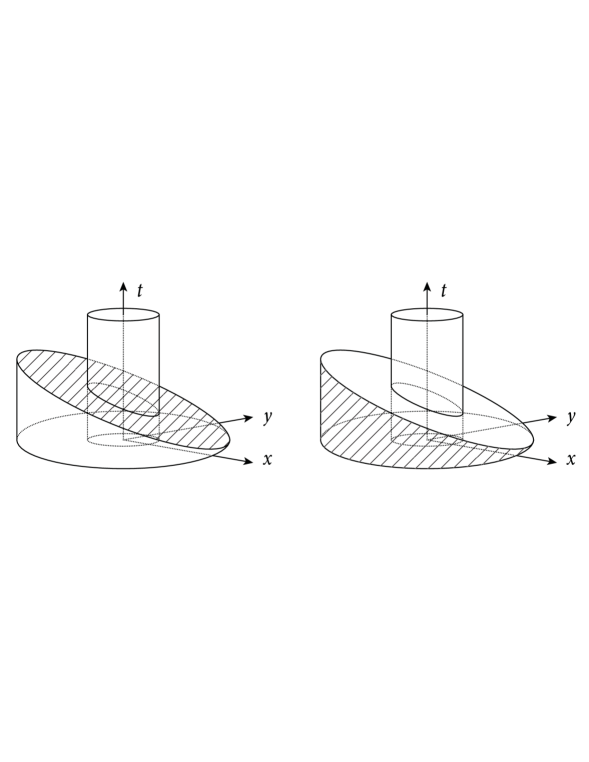
Figure 5: Two of the many possible spacetime areas associated with the spacetime loop, $\oint A_{\mu}dx^{\mu}$. The spacetime area on the left hand side (i.e. the slanted top of the spacetime cylinder) gets a contribution only from the magnetic field. The spacetime area on the right hand side (i.e. the side of the spacetime cylinder) gets a contribution only from the electric field.

We now calculate the right hand side of Stokes’ theorem – the field version of the spacetime area integral, $\frac{1}{2}\int F_{\mu\nu}d\sigma^{\mu\nu}=\int{\bf E}\cdot d{\bf x}~{}cdt+\int{\bf B}\cdot d{\bf a}$. In this case, we use the two spacetime surfaces shown in Fig. (5), both of which span the spacetime path used in evaluating $\oint A_{\mu}dx^{\mu}$.

For the spacetime area that is the side of the spacetime cylinder – the right side of Fig. (5) – only the electric field will contribute i.e. $\frac{1}{2}\int F_{\mu\nu}d\sigma^{\mu\nu}\rightarrow\int{\bf E}\cdot d{\bf x}~{}cdt$. We can obtain this electric piece using our results from (46) and (49) with $\varphi_{0}=2\pi$, but with one subtlety: we need to reverse the signs relative to those given in (46) and (49) so that we have

$$\int_{1}{\bf E}\cdot d{\bf x}~{}cdt=+\frac{B_{0}R^{2}\pi^{2}}{4\omega}~{}~{}~{}~{};~{}~{}~{}~{}\int_{4}{\bf E}\cdot d{\bf x}~{}cdt=-\frac{B_{0}R^{2}\pi^{2}}{4\omega}.$$ (26)

The reason for the sign reversal is as follows: when we form a closed spacetime loop from the two contours in Fig. (3), the direction of the spacetime loop is counterclockwise when the solenoid is viewed from above. As previously mentioned, this is the reverse of the paths in Fig. (2). For purely spatial examples of Stokes’ theorem, reversing the direction of traversal for the path reverses the direction of the 3-vector area via the right-hand-rule. Here, although there is no equivalent right-hand-rule for the spacetime area, we nevertheless need to reverse the spacetime area “direction” when the closed spacetime path is traversed in the opposite direction. This might be viewed as an extension of the right-hand-rule to spacetime paths and areas. One can obtain this result on the “direction” of the spacetime area less heuristically using differential forms and wedge product notation. Reviewing differential forms and wedge product notation is outside the scope of this article, but the interested reader can find nice expositions on this in the textbooks by Frankel frankel , Felsager felsager and Ryder. ryder To get the spacetime area contribution associated with the closed spacetime loop in Fig. (3), we apply the time-reversal operator to area 4, which changes the sign of $\int\int_{4}{\bf E}\cdot d{\bf x}~{}cdt$ since ${\bf E}$ and $d{\bf x}$ are even under time reversal, but $dt$ is odd. We then add the time reversed result for path 4 to the result for area 1 which gives

$$\int{\bf E}\cdot d{\bf x}dt=\left(\int_{1}+T\int_{4}\right){\bf E}\cdot d{\bf x}~{}cdt=\frac{B_{0}R^{2}\pi^{2}}{2\omega}~{}.$$ (27)

This result agrees with the results for the loop integral for the 4-vector potentials in the two different gauges, given in (20) and (25).

We now calculate $\frac{1}{2}\int F_{\mu\nu}d\sigma^{\mu\nu}$ for the spacetime area on the left hand side of Fig. (5) i.e. the slanted “top” of the spacetime cylinder. For this spacetime area, only the magnetic field contributes i.e. $\frac{1}{2}\int F_{\mu\nu}d\sigma^{\mu\nu}\rightarrow\int{\bf B}\cdot d{\bf a}$. For the previous case, shown in Fig. (2), our spacetime loop enclosed a region where ${\bf B}=0$. Now from the right hand side of Fig. (5) we can see that the spacetime area will have ${\bf B}\neq 0$ so we expect $\int{\bf B}\cdot d{\bf a}\neq 0$. For the spacetime area associated with path 1 we have

$$\int_{0}^{\pi}\int_{0}^{R}{\bf B}\cdot{\hat{\bf z}}\rho d\rho d\varphi=\frac{B_{0}R^{2}}{2\omega}\int_{0}^{\pi}\varphi d\varphi=\frac{B_{0}R^{2}\pi^{2}}{4\omega}~{},$$ (28)

where we have used $t=\varphi/\omega$ to write the magnetic field magnitude as $B_{0}t\rightarrow B_{0}\varphi/\omega$. Note that here the area vector points along the positive z-axis $d{\bf a}={\hat{\bf z}}\rho d\rho d\varphi$. For the spacetime area associated with segment 4 we have

$$\int_{0}^{-\pi}\int_{0}^{R}{\bf B}\cdot(-{\hat{\bf z}})\rho d\rho d\varphi=-\frac{B_{0}R^{2}}{2\omega}\int_{0}^{-\pi}\varphi d\varphi=-\frac{B_{0}R^{2}\pi^{2}}{4\omega}~{}.$$ (29)

Again we have used $t=\varphi/\omega$ and $d\varphi=\omega dt$. Here the area vector points along the negative z-axis ($d{\bf a}=-{\hat{\bf z}}\rho d\rho d\varphi$) since the path is traversed in a clockwise direction. To get the spacetime area associated with the closed spacetime loop, we add the result of (28) to the time reversed result of (29)

$$\int{\bf B}\cdot d{\bf a}=\int_{1}{\bf B}\cdot d{\bf a}+T\left[\int_{4}{\bf B}\cdot d{\bf a}\right]=\int_{1}{\bf B}\cdot d{\bf a}-\int_{4}{\bf B}\cdot d{\bf a}=\frac{B_{0}R^{2}\pi^{2}}{2\omega}~{}.$$ (30)

This result agrees with the results for the loop integrals for the 4-vector potentials in the two different gauges given in (20) and (25), and agrees with the result for the spacetime area integral from (27). This is reminiscent of the charging capacitor demonstration of Maxwell’s displacement current. d-current In this example, there is a circular loop that encloses a wire which is charging up a capacitor. The closed loop integral of the magnetic field (i.e. $\oint{\bf B}\cdot d{\bf x}$) gives ${\bf B}\propto\frac{I(t)}{\rho}{\hat{\boldsymbol{\varphi}}}$. If the surface chosen to span this loop cuts through the wire then $I(t)$ is the current due to charges. However, the surface can be chosen so that it goes between the capacitor plates where one has no current from charges. In this region one does have a time-changing electric field and so the contribution to the magnetic field loop integral now comes from the displacement current. Here, the loop integral of the vector potential is related to the spacetime area integral of the electric field in one case, and related to the spacetime area integral of the magnetic field in the other case.

III Summary and Conclusions

In this work, we have given explicit examples of Stokes’ theorem in the case where there exists time-dependent fields (i.e. 4D Stokes’ theorem). There are many examples of Stokes’ theorem as it applies to time-independent fields (i.e. 3D Stokes’ theorem), but these are perhaps the first explicit worked out examples of Stokes’ theorem with time-dependent fields. In fact, there are some claims that Stokes’ theorem does not apply to time-dependent fields (see the first footnote on page 305 and the first paragraph on page 312 of reference brown ). Despite these assertions, we have found that Stokes’ theorem can be applied to time-dependent cases if care is taken in how the spacetime loop is closed. In particular we investigated an infinite solenoid with a linearly increasing magnetic flux. There we showed $\oint A_{\mu}dx^{\mu}=\frac{1}{2}\int F_{\mu\nu}d\sigma^{\mu\nu}$ for the spacetime loop closed outside the solenoid – see Fig. (2). We also showed that $\oint A^{\prime}_{\mu}dx^{\mu}$, for the closed spacetime loop from Fig. (2), remained the same for a gauge transformed 4-potential as given in (13) (14), demonstrating the gauge invariance of $\oint A_{\mu}dx^{\mu}$.

We also investigated the more subtle case when the spacetime loop enclosed the solenoid. Here we also calculated $\oint A_{\mu}dx^{\mu}$ in the two gauges given in (10) and (13) (14). For the 4-vector potential (obtained with the multi-valued gauge function $\chi$) given in (13) (14), we had to excise the singularity at $\rho=0$ via the contour given in Fig. (4). In terms of the spacetime area integral of the fields we carried out the calculation using the two spacetime areas given in Fig. (5): (i) the side of the spacetime cylinder where only the electric field contributed; (ii) the slanted top of the spacetime cylinder where only the magnetic field contributed. The result of $\frac{1}{2}\int F_{\mu\nu}d\sigma^{\mu\nu}$ came either from the side spacetime area or the slanted top spacetime area. This is similar to the standard example used to demonstrate Maxwell’s displacement current.

The time-dependent Stokes’ theorem is closely related to the time dependent Aharonov-Bohm effect and the the discussion in this article has been closely guided by this connection. The spacetime contours from Figs. (2) (3) were taken to be those that a real particle could traverse since this is what occurs in the Aharonov-Bohm effect. Although much work has been done on the time-independent Aharonov-Bohm effect, much less has been done in regard to the time-dependent Aharonov-Bohm effect. There are only two experiments that we have found which have been done on the time-dependent Aharonov-Bohm effect – one accidental experiment marton and one purposeful experiment. ageev Two theoretical papers werner ; macdougall2 were written in an attempt to explain the surprising non-result of the accidental experiment of Marton et al. marton More recently, there have been some theoretical papers chiao ; singleton ; bright dealing with the time-dependent Aharonov-Bohm effect. Still, aside from the two experiments in marton ; ageev (both of which gave unclear results), there is little in the way of experimental results for the time-dependent Aharonov-Bohm effect.

As a final comment we note that the electric field associated with the solenoid, given in (12), is of the form one would expect for a current of magnetic charges – just as a current of electric charges produces a magnetic field of the form ${\bf B}\propto\frac{1}{\rho}{\hat{\boldsymbol{\varphi}}}$, so too a current of magnetic charges would produce an electric field of the form ${\bf E}\propto\frac{1}{\rho}{\hat{\boldsymbol{\varphi}}}$. This connection to magnetic charge also offers another example of a non-single valued gauge transformation. The following 3-vector potential (we now use spherical polar coordinates $r,\theta,\varphi$, rather than the cylindrical coordinates, $\rho,\varphi,z$) yields a monopole magnetic field ${\bf B}=\nabla\times{\bf A}=g{\hat{\bf r}}/r^{2}$

$${\bf A}_{{\rm monopole}}=\frac{g(1-\cos\theta)}{r\sin\theta}{\hat{\boldsymbol{\varphi}}}~{}.$$ (31)

The vector potential in (31) is single valued, but it has the usual Dirac string singularity pathology along the negative z-axis i.e. $\theta=\pi$. One can also obtain a magnetic monopole field from ${\bf A}_{monopole}=-\frac{g(1+\cos\theta)}{r\sin\theta}{\hat{\boldsymbol{\varphi}}}$ which has a Dirac string singularity along the positive z-axis i.e. $\theta=0$. These two forms of the monopole 3-vector potential are related by the gauge transformation ${\bf A}\rightarrow{\bf A}-\nabla\chi$ with $\chi=2g\varphi$. In this case the gauge function $\chi$ is non-single valued, but the two forms of the gauge potential ${\bf A}_{{\rm monopole}}$ are single valued. Thus, this is not exactly like the 4-potentials and gauge transformation for the time-dependent solenoid case, given in (13) (14) and (15), where both the potentials and gauge function were non-single valued.

It is easy to see that one can also get a magnetic monopole field from the following alternative 3-vector potential arfken ; pal ; macdougall

$${\bf A}_{{\rm monopole}}=-\frac{g\varphi\sin\theta}{r}{\hat{\boldsymbol{\theta}}}~{},$$ (32)

which does not have the Dirac string singularity of (31), but is non-single valued due to the $\varphi$ dependence of $A_{\theta}$. The two vector potentials in (31) and (32) are related by a gauge transformation of the form

$$A^{\mu}\rightarrow A^{\mu}+\partial^{\mu}\chi~{}~{}~{};~{}~{}~{}\chi=-g(1-\cos\theta)\varphi$$ (33)

Here we see that both the gauge transformation function $\chi$ in (33) and the 3-vector gauge potential (32) are non-single valued, which then is similar to the situation for the time-dependent solenoid as given in (13) , (14), (15).

Acknowledgments: DS is supported by a 2015-2016 Fulbright Scholars Grant to Brazil and by grant $\Phi.0755$ in fundamental research in natural sciences by the Ministry of Education and Science of Kazakhstan. DS wishes to thank the ICTP-SAIFR in São Paulo for it hospitality. We gratefully acknowledge Joe Deutscher for help with the figures in the paper.

Appendix I

In this appendix we carry out the details of the 6 line integrals for $\oint A_{\mu}dx^{\mu}$ with the 4-vector potential from (10). For path 1, the vector potential from (10) is ${\bf A}=\frac{B_{0}tR^{2}}{2\rho_{1}}{\hat{\boldsymbol{\varphi}}}$ since the radius on this path is $\rho_{1}$. The infinitesimal path length element is $d{\bf x}=\rho_{1}d\varphi{\hat{\boldsymbol{\varphi}}}$. The path is traversed at a constant angular speed $\omega$ so that we have the relationship $\varphi=\omega t\rightarrow d\varphi=\omega dt$. The particle starts at $\varphi=0$ and $t=0$ and ends at $\varphi=\frac{\varphi_{0}}{2}$ at $t=\frac{\varphi_{0}}{2\omega}$, yielding

$$\int_{1}{\bf A}\cdot d{\bf x}=\frac{B_{0}R^{2}}{2}\int_{0}^{\varphi_{0}/2}td\varphi=\frac{B_{0}R^{2}\omega}{2}\int_{0}^{\varphi_{0}/2\omega}tdt=\frac{B_{0}R^{2}\varphi_{0}^{2}}{16\omega}$$ (34)

For path 2 we have ${\bf A}=\frac{B_{0}tR^{2}}{2\rho}{\hat{\boldsymbol{\varphi}}}$ (now $\rho$ varies) and $d{\bf x}=d\rho{\hat{\boldsymbol{\rho}}}$. Thus ${\bf A}\cdot d{\bf x}=0$ and we get no contribution to the loop integral from this line segment. We have taken the velocity along path 2 to be the same as the velocity along path 1 (namely $\rho_{1}\omega$) and the distance traveled is $\rho_{2}-\rho_{1}$ (the distance from line segment 1 to line segment 3). Thus for path 2 we have

$$\int_{2}{\bf A}\cdot d{\bf x}\propto\int_{2}{\hat{\boldsymbol{\varphi}}}\cdot{\hat{\boldsymbol{\rho}}}d\rho=0~{}.$$ (35)

Although the line integral for path 2 is zero, time passes in the traversal of the path. This will have an effect on the result for line segment 3. The amount of time that passes during the traversal of path 2 is $\Delta t_{2}=\frac{\rho_{2}-\rho_{1}}{\rho_{1}\omega}$. For path 3 from (10) we have ${\bf A}=\frac{B_{0}tR^{2}}{2\rho_{2}}{\hat{\boldsymbol{\varphi}}}$, since the radius on this path is $\rho_{2}$. The infinitesimal length element is $d{\bf x}=-\rho_{2}d\varphi{\hat{\boldsymbol{\varphi}}}$. The path is traversed at a constant angular speed $\omega^{\prime}=\omega\frac{\rho_{1}}{\rho_{2}}$ (the angular speed is slower) but this ensures that the linear speed along paths 1, 2 and 3 is the same . We now have the relationship $\varphi=\omega^{\prime}t\rightarrow d\varphi=\omega^{\prime}dt$. The particle starts at $\varphi=\frac{\varphi_{0}}{2}$ and $t_{i}=\frac{\varphi_{0}}{2\omega}+\frac{\rho_{2}-\rho_{1}}{\rho_{1}\omega}$ (this offset time $\frac{\rho_{2}-\rho_{1}}{\rho_{1}\omega}$ is connected with the traversal of path 2). The particle ends at $\varphi=0$ at $t_{f}=t_{i}+\frac{\varphi_{0}}{2\omega^{\prime}}$, yielding

$$\int_{3}{\bf A}\cdot d{\bf x} = -\frac{B_{0}R^{2}}{2}\int_{t_{i}}^{t_{f}}td\varphi=-\frac{B_{0}R^{2}\omega^{\prime}}{2}\int_{t_{i}}^{t_{f}}tdt=-\frac{B_{0}R^{2}\omega^{\prime}}{4}t^{2}{\bigg{|}}_{t_{i}}^{t_{f}}$$ (36)

$$= -\frac{B_{0}R^{2}\varphi_{0}^{2}}{16\omega}\left[\frac{\rho_{2}}{\rho_{1}}+\frac{4(\rho_{2}-\rho_{1})}{\rho_{1}\varphi_{0}}+2\right]$$

Next we calculate $\int{\bf A}\cdot d{\bf x}$ for line segments 4, 5 and 6. The integral $\int_{4}{\bf A}\cdot d{\bf x}$ is the same as $\int_{1}{\bf A}\cdot d{\bf x}$ except $d{\bf x}=-\rho_{1}d\varphi{\hat{\boldsymbol{\varphi}}}$ which changes the final result by a sign

$$\int_{4}{\bf A}\cdot d{\bf x}=-\frac{B_{0}R^{2}\varphi_{0}^{2}}{16\omega}$$ (37)

The integral $\int_{5}{\bf A}\cdot d{\bf x}$, like $\int_{2}{\bf A}\cdot d{\bf x}$ is zero since

$$\int_{5}{\bf A}\cdot d{\bf x}\propto\int_{5}{\hat{\boldsymbol{\varphi}}}\cdot{\hat{\boldsymbol{\rho}}}d\rho=0~{}.$$ (38)

Again time $\Delta t_{5}=\frac{\rho_{2}-\rho_{1}}{\rho_{1}\omega}$ passes during the traversal of path 5, affecting the result of path 6. Finally, path 6 is similar to path 3 except $d{\bf x}=\rho_{2}d\varphi{\hat{\boldsymbol{\varphi}}}$ which changes the final overall sign. Similar to path 3, path 6 is traversed at a constant angular speed $\omega^{\prime}=\omega\frac{\rho_{1}}{\rho_{2}}$ which ensures that the linear speed along path 6 and path 4 are the same (in fact the speed along all six segments is taken to be the same). As before, we have the relationship $\varphi=\omega^{\prime}t\rightarrow d\varphi=\omega^{\prime}dt$. The particle starts at $\varphi=-\frac{\varphi_{0}}{2}$ and $t_{i}=\frac{\varphi_{0}}{2\omega}+\frac{\rho_{2}-\rho_{1}}{\rho_{1}\omega}$ and ends at $\varphi=0$ and $t_{f}=t_{i}+\frac{\varphi_{0}}{2\omega^{\prime}}$, yielding

$$\int_{6}{\bf A}\cdot d{\bf x}=\frac{B_{0}R^{2}\varphi_{0}^{2}}{16\omega}\left[\frac{\rho_{2}}{\rho_{1}}+\frac{4(\rho_{2}-\rho_{1})}{\rho_{1}\varphi_{0}}+2\right]$$ (39)

Notice that the result for path 6 is equivalent to the negative of path 3.

Appendix II

In this appendix we carry out the details of the 6 line segment integrals for $\oint A_{\mu}dx^{\mu}$ for the 4-vector potential from (13). For path 1 we have

$$\int_{1}\phi^{\prime}cdt=\frac{B_{0}R^{2}}{2}\int_{0}^{\varphi_{0}/2\omega}\varphi dt=\frac{B_{0}R^{2}\omega}{2}\int_{0}^{\varphi_{0}/2\omega}tdt=\frac{B_{0}R^{2}\varphi_{0}^{2}}{16\omega}~{},$$ (40)

where we use $\varphi=\omega t$. For path 2, the scalar potential is constant $\phi^{\prime}=\frac{B_{0}R^{2}\varphi_{0}}{4}$ and the time to traverse path 2 is, as in Appendix I, $\Delta t=\frac{\rho_{2}-\rho_{1}}{\rho_{1}\omega}$. So for path 2 we have

$$\int_{2}\phi^{\prime}cdt=\frac{B_{0}R^{2}\varphi_{0}}{4}\int_{0}^{\Delta t}dt=\frac{B_{0}R^{2}\varphi_{0}}{4}\left(\frac{\rho_{2}-\rho_{1}}{\rho_{1}\omega}\right)~{}.$$ (41)

For path 3 we use the relationship $\varphi=\frac{\varphi_{0}}{2}-\omega^{\prime}t$. The integral is

$$\int_{3}\phi^{\prime}cdt=\frac{B_{0}R^{2}}{2}\int_{0}^{\varphi_{0}/2\omega^{\prime}}\varphi dt=\frac{B_{0}R^{2}}{2}\left(\frac{\varphi_{0}}{2}t-\frac{1}{2}\omega^{\prime}t^{2}\right){\bigg{|}}_{0}^{\varphi_{0}/2\omega^{\prime}}=\frac{B_{0}R^{2}\varphi_{0}^{2}\rho_{2}}{16\omega\rho_{1}}.$$ (42)

Next we calculate $\int\phi^{\prime}cdt$ for line segments 4, 5, and 6. Line segment 4 is similar to path 1 except that $\varphi=-\omega t$ which then changes the sign of the result

$$\int_{4}\phi^{\prime}cdt=-\frac{B_{0}R^{2}\varphi_{0}^{2}}{16\omega}~{}.$$ (43)

Path 5 is similar to path 2 except now the scalar potential takes a different constant value $\phi^{\prime}=-\frac{B_{0}R^{2}\varphi_{0}}{4}$.

$$\int_{5}\phi^{\prime}cdt=-\frac{B_{0}R^{2}\varphi_{0}}{4}\left(\frac{\rho_{2}-\rho_{1}}{\rho_{1}\omega}\right)~{}.$$ (44)

Path 6 is similar to path 3 except now we have $\varphi=-\frac{\varphi_{0}}{2}+\omega^{\prime}t$. The integral is

$$\int_{6}\phi^{\prime}cdt=-\frac{B_{0}R^{2}\varphi_{0}^{2}\rho_{2}}{16\omega\rho_{1}}.\\$$ (45)

Appendix III

In this appendix we carry out details of the spacetime area integral of the electric and magnetic fields for the spacetime loop given in Fig. 2

For the spacetime area connected with path 1, the electric field and infinitesimal line element are ${\bf E}=-\frac{B_{0}R^{2}}{2c\rho_{1}}{\hat{\boldsymbol{\varphi}}}$ and $d{\bf x}=\rho_{1}d\varphi{\hat{\boldsymbol{\varphi}}}$ respectively, so

$$\int_{1}{\bf E}\cdot d{\bf x}~{}cdt=-\int_{0}^{\varphi_{0}/2\omega}dt\int_{0}^{\omega t}\frac{B_{0}R^{2}}{2}d\varphi=-\int_{0}^{\varphi_{0}/2\omega}\left(\frac{B_{0}R^{2}\omega t}{2}\right)dt=-\frac{B_{0}R^{2}\varphi_{0}^{2}}{16\omega}~{}.$$ (46)

For the spacetime area connected with path 2, the electric field is ${\bf E}=-\frac{B_{0}R^{2}}{2c\rho}{\hat{\boldsymbol{\varphi}}}$ – now the radial coordinate $\rho$ is not fixed at $\rho=\rho_{1}$ but rather runs from $\rho_{1}$ to $\rho_{2}$. The infinitesimal line element is $d{\bf x}=\rho d\varphi{\hat{\boldsymbol{\varphi}}}$ so that for each $\rho$ along path 2 (with $\rho_{1}\leq\rho\leq\rho_{2}$) the $d\varphi$ integration runs from $\varphi=0$ to $\varphi=\varphi_{0}/2$. The integration over $dt$ runs from $t=0$ to $t=\frac{\rho_{2}-\rho_{1}}{\rho_{1}\omega}$ which corresponds to moving from $\rho_{1}$ to $\rho_{2}$ at a speed of $\rho_{1}\omega$. The $dt$ integration in combination with the $d\varphi$ integration sweeps out the spacetime area. Thus for path 2 the spacetime area integral is

$$\int_{2}{\bf E}\cdot d{\bf x}~{}cdt = -\int_{0}^{\frac{\rho_{2}-\rho_{1}}{\rho_{1}\omega}}dt\int_{0}^{\varphi_{0}/2}\frac{B_{0}R^{2}}{2}d\varphi$$ (47)

$$= -\int_{0}^{\frac{\rho_{2}-\rho_{1}}{\rho_{1}\omega}}\left(\frac{B_{0}R^{2}\varphi_{0}}{4}\right)dt=-\frac{B_{0}R^{2}\varphi_{0}^{2}}{4\rho_{1}\omega}(\rho_{2}-\rho_{1})~{}.$$

For the spacetime area connected with path 3 the electric field is ${\bf E}=-\frac{B_{0}R^{2}}{2c\rho_{2}}{\hat{\boldsymbol{\varphi}}}$ and the infinitesimal line element is $d{\bf x}=\rho_{2}d\varphi{\hat{\boldsymbol{\varphi}}}$. The $d\varphi$ integration goes from $\varphi=0$ to $\varphi=\frac{\varphi_{0}}{2}-\omega^{\prime}t$ (the angular velocity is $\omega^{\prime}=\frac{\rho_{1}}{\rho_{2}}\omega$ so that the linear speed is the same on each path). The $dt$ integration runs from $t=0$ to $t=\varphi_{0}/2\omega^{\prime}$. Thus the spacetime integral connected with path 3 is

$$\int_{3}{\bf E}\cdot d{\bf x}~{}cdt = -\int_{0}^{\varphi_{0}/2\omega^{\prime}}dt\int_{0}^{\frac{\varphi_{0}}{2}-\omega^{\prime}t}\frac{B_{0}R^{2}}{2}d\varphi$$ (48)

$$= -\int_{0}^{\varphi_{0}/2\omega^{\prime}}\frac{B_{0}R^{2}}{2}\left(\frac{\varphi_{0}}{2}-\omega^{\prime}t\right)dt=-\frac{B_{0}R^{2}\varphi_{0}^{2}\rho_{2}}{16\omega\rho_{1}}~{}.$$

The spacetime area integration connected with path 4 is similar to the integration connected with path 1, except here the limits on the $d\varphi$ integration run from $\varphi=0$ to $\varphi=-\omega t$, yielding

$$\int_{4}{\bf E}\cdot d{\bf x}cdt=-\int_{0}^{\varphi_{0}/2\omega}dt\int_{0}^{-\omega t}\frac{B_{0}R^{2}}{2}d\varphi=\int_{0}^{\varphi_{0}/2\omega}\left(\frac{B_{0}R^{2}\omega t}{2}\right)dt=\frac{B_{0}R^{2}\varphi_{0}^{2}}{16\omega}~{}.$$ (49)

Note by comparing (46) and (49) one sees $\int_{4}{\bf E}\cdot d{\bf x}cdt=-\int_{1}{\bf E}\cdot d{\bf x}cdt$. The spacetime area integration connected with path 5 is similar to the integration connected with path 2, except the limits on the $d\varphi$ integration run from $\varphi=0$ to $\varphi=-\varphi_{0}/2$, yielding

$$\int_{5}{\bf E}\cdot d{\bf x}~{}cdt = -\int_{0}^{\frac{\rho_{2}-\rho_{1}}{\rho_{1}\omega}}dt\int_{0}^{-\varphi_{0}/2}\frac{B_{0}R^{2}}{2}d\varphi$$ (50)

$$= \int_{0}^{\frac{\rho_{2}-\rho_{1}}{\rho_{1}\omega}}\left(\frac{B_{0}R^{2}\varphi_{0}}{4}\right)dt=\frac{B_{0}R^{2}\varphi_{0}^{2}}{4\rho_{1}\omega}(\rho_{2}-\rho_{1})~{}.$$

Note that comparing (47) and (50) illustrated that $\int_{5}{\bf E}\cdot d{\bf x}cdt=-\int_{2}{\bf E}\cdot d{\bf x}cdt$. Finally, the spacetime area integration connected with path 6 is similar to the integration connected with path 3, except here the limits on the $d\varphi$ integration run from $\varphi=0$ to $\varphi=\omega^{\prime}t-\varphi_{0}/2$.

$$\int_{6}{\bf E}\cdot d{\bf x}~{}cdt = -\int_{0}^{\varphi_{0}/2\omega^{\prime}}dt\int_{0}^{\omega^{\prime}t-\frac{\varphi_{0}}{2}}\frac{B_{0}R^{2}}{2}d\varphi$$ (51)

$$= -\int_{0}^{\varphi_{0}/2\omega^{\prime}}\frac{B_{0}R^{2}}{2}\left(\omega^{\prime}t-\frac{\varphi_{0}}{2}\right)dt=\frac{B_{0}R^{2}\varphi_{0}^{2}\rho_{2}}{16\omega\rho_{1}}~{}.$$

Again note that comparing (48) and (51) illustrates that $\int_{6}{\bf E}\cdot d{\bf x}cdt=-\int_{3}{\bf E}\cdot d{\bf x}cdt$.

As a final comment, the “direction” of the spacetime area associated with the closed spacetime paths of Fig. (2) or Fig. (3) does not have a well known right hand rule as is the case for purely spatial contours and areas. The directionality that we have chosen above for the spacetime area is taken so that the area integral of the fields in (18) agrees with the results of the contour integrals of the two vector potentials given in (16) and (17) for the closed contour given in Fig. (2) (i.e. this choice ensures that Stokes’ theorem works out for Fig. (2)). In contrast, for the path which encloses the solenoid in Fig. (3) the direction in which the path is traversed, and thus the spacetime “area” direction, is reversed relative to the path in Fig (2). Thus the spacetime area associated with the contour in Fig. (3) must have the opposite sign from the spacetime area which comes from the contour in Fig. (2). This again ensures that Stokes’ theorem works out for the contour which encloses the solenoid. One can regard the procedure described above, with the determining of the “direction” of the spacetime area based on the direction in which the closed spacetime contour closes (clockwise or counterclockwise) as an extension of the right hand rule to spacetime contours and surfaces. A more rigorous way to determine the direction of the area for mixed spatial and time surfaces is given through the use of differential forms ryder ; frankel ; felsager .

References

- (1) Y. Aharonov and D. Bohm, “Significance of electromagnetic potentials in the quantum theory”, Phys. Rev. 115, 485-491 (1959).
- (2) L. Ryder, Quantum Field Theory 2nd edition, (Cambridge University Press, Cambridge UK 1996).
- (3) J. Macdougall and D. Singleton, “Stokes’ theorem, gauge symmetry and the time-dependent Aharonov-Bohm effect”, J. Math. Phys. 55, 042101 (2014).
- (4) T.A. Abbott and D.J. Griffiths, “Acceleration without radiation”, Am. J. Phys. 53 1203-1211 (1985).
- (5) D. Singleton and E. Vagenas, “The covariant, time-dependent Aharonov-Bohm Effect”, Phys. Lett. B 723, 241-244 (2013).
- (6) J.D. Jackson, Classical Electrodynamics, 3rd edition, section 6.10 (John Wiley & Sons Inc., New York).
- (7) T. Frankel, The Geometry of Physics: An Introduction, edition (Cambridge University Press, Cambridge UK 2012).
- (8) B. Felsager, Geometry, Particles, and Fields, (Springer-Verlag Press, New York, NY 1997).
- (9) D. J. Griffiths Introduction to Electrodynamics, 3rd edition, section 7.3 (Prentice Hall, Upper Saddle River, NJ 1999).
- (10) R. A. Brown and D. Home, “Locality and Causality in Time-Dependent Aharonov-Bohm Interference”, Nuovo Cimento B 107, 303-316 (1992).
- (11) L. Marton, J. A. Simpson, and J. A. Suddeth, “An Electron Interferometer”, Rev. Sci. Instr. 25, 1099-1104 (1954).
- (12) A. N. Ageev, S. Yu. Davydov, and A. G. Chirkov, “Magnetic Aharonov-Bohm Effect under Time-Dependent Vector Potential”, Technical Phys. Letts. 26, 392-393 (2000).
- (13) F.G. Werner and D. Brill, “Significance of Electromagnetic Potentials in the Quantum Theory in the Interpretation of Electron Interferometer Fringe Observations”, Phys. Rev. Letts., 4, 344-347 (1960).
- (14) J. Macdougall, D. Singleton, and E. C. Vagenas, “Revisiting the Marton, Simpson, and Suddeth experimental confirmation of the Aharonov–Bohm effect”, Phys. Lett. A 379, 1689-1692 (2015).
- (15) B. Lee, E. Yin, T. K. Gustafson, and R. Chiao, “Analysis of Aharonov–Bohm effect due to time-dependent vector potentials”, Phys. Rev. A 45, 4319-4325 (1992).
- (16) M. Bright, D. Singleton and A. Yoshida, “Aharonov–-Bohm phase for an electromagnetic wave background”, Eur. Phys. J. C 75, 446 (2015).
- (17) G. B. Arfken, H-J. Weber: “Mathematical Methods for Physicists” (Harcourt/Academic Press), 5th Edition, page 130.
- (18) R.K. Ghosh and P.B. Pal, “A non-singular potential for the Dirac monopole”, Phys. Lett. B 551, 387-390 (2003).