Asymptotics for the ruin time of a piecewise exponential Markov process with jumps

Abstract

In this paper a class of Ornstein–Uhlenbeck processes driven by compound Poisson processes is considered. The jumps arrive with exponential waiting times and are allowed to be two-sided. The jumps are assumed to form an iid sequence with distribution a mixture (not necessarily convex) of exponential distributions, independent of everything else. The fact that downward jumps are allowed makes passage of a given lower level possible both by continuity and by a jump. The time of this passage and the possible undershoot (in the jump case) is considered. By finding partial eigenfunctions for the infinitesimal generator of the process, an expression for the joint Laplace transform of the passage time and the undershoot can be found.

From the Laplace transform the ruin probability of ever crossing the level can be derived. When the drift is negative this probability is less than one and its asymptotic behaviour when the initial state of the process tends to infinity is determined explicitly.

The situation where the level to cross decreases to minus infinity is more involved: The level to cross plays a much more fundamental role in the expression for the joint Laplace transform than the initial state of the process. The limit of the ruin probability in the positive drift case and the limit of the distribution of the undershoot in the negative drift case is derived.

Keywords: Asymptotic ruin probabilities; Integration contour; Ornstein–Uhlenbeck process; Partial Eigenfunction; Shot–noise process

1 Introduction

The main aim of this paper is to determine the asymptotic behaviour of the ruin probability for a certain class of time–homogeneous Markov processes with jumps. These processes, referred to as $X$ below, can be viewed as Ornstein–Uhlenbeck processes satisfying

$${\mathrm{d}}X_{t}=\kappa X_{t}\,{\mathrm{d}}t+{\mathrm{d}}U_{t}\,,$$ (1)

driven by a compound Poisson process $(U_{t})$. The ruin time, $\tau(\ell)$, is defined as the time to passage below $\ell$ for an initial state $x>\ell$. The passage below $\ell$ can be a result of a downward jump, and in some cases a continuous passage through $\ell$ is is also possible. The main results give asymptotic descriptions of $\mathbb{P}^{x}(\tau(\ell)<\infty)$, when $\kappa>0$ in the limits $x\to\infty$ and $\ell\to-\infty$. Furthermore, the limit distribution of the undershoot in case of passage by jump is determined for $\kappa<0$ and $\ell\to-\infty$.

It will be assumed that the driving compound Poisson process has a special jump structure. Both the downward and upward jumps are assumed to have a density (not the same) that is a linear – not necessarily convex – combination of exponential densities

It is important to distinguish between two different scenarios: Whether the drift $\kappa$ is positive, hence $X$ is transient, or the drift is negative, in which case the process $X$ is recurrent. In the negative drift case the probability $\mathbb{P}^{x}(\tau(\ell)<\infty)$ (with $\tau(\ell)$ denoting the time of passage) of ever crossing below $\ell$ when starting at $x$ is always 1. When the drift $\kappa$ is positive we have that $\mathbb{P}^{x}(\tau(\ell)<\infty)<1$, and this probability decreases when either $x\to\infty$ or $\ell\to-\infty$.

The distribution of the passage time (and by that also the ruin probability) is determined through the Laplace transform. This is found by exploiting certain stopped martingales derived from using bounded partial eigenfunctions for the infinitesimal generator for $X$. An explicit expression for the Laplace transform is determined in [10]. Here the partial eigenfunctions are found as linear combinations of functions given by contour integrals in the complex plane. Also the Laplace transform ends up being a linear combination of these integrals. It is the resulting Laplace transform from [10] that we shall investigate in this paper.

In the present paper the asymptotics of $\mathbb{P}^{x}(\tau(\ell)<\infty)$ is explored in both of the situations $x\to\infty$ and $\ell\to-\infty$. This becomes a question about finding the asymptotics for the complex contour integrals mentioned above. It turns out that the $\ell\to-\infty$ problem is the far most complicated because the dependence of $\ell$ in the construction of the partial eigenfunctions is more involved. Nevertheless, the need of exploring the asymptotic behaviour of the integrals is similar. When $x\to\infty$ we see that $\mathbb{P}^{x}(\tau(\ell)<\infty)$ decreases exponentially (adjusted by some specified power function) with the exponential parameter from the leading exponential part of the downward jumps.

The technique of using partial eigenfunctions for the infinitesimal generator has appeared before. Paulsen and Gjessing, [13], considers a model like the present, but in the more general (and also different) setup

$$dX_{t}=(p+\kappa X_{t})\,dt-dU_{t}+\sqrt{\sigma_{1}^{2}+\sigma_{2}^{2}X_{t}^{2}}\,dB_{t}\,+X_{t}d\tilde{U}_{t}\,.$$ (2)

Here both $U$ and $\tilde{U}$ are compound Poisson processes of the form $\sum_{n=1}^{N_{t}}V_{n}$. In [13] it is shown that a partial eigenfunction for the corresponding infinitesimal generator for (2) will lead to the ruin probability and also the Laplace transform for the ruin time. [5] shows in a model without $\sigma_{1}^{2}$ and $\tilde{U}$ the existence of this partial eigenfunction under some smoothness assumptions about the jump distributions in $U$. This result is extended to weaker assumptions in [6].

In the case of $\sigma_{1}^{2}=\sigma_{2}^{2}=0$, without $\tilde{U}$, and assuming exponential negative jump and no positive jumps, an explicit formula for the Laplace transform is determined in [13]. Furthermore, the exponential decrease in $\mathbb{P}^{x}(\tau(\ell)<\infty)$ is derived in the $x\to\infty$ asymptotic situation for some fixed $0<\ell<x$. For the case of exponential negative jumps also see Asmussen [1], Chapter VII.

In the present paper the jump distributions are assumed to be light tailed. The existing literature does not contain very explicit results for the asymptotic ruin probability with that kind of jump distributions. In [4] and [14] it is proved in the $\sigma_{2}^{2}=0$ case with $\kappa=\sup\{a\;|\;\mathbb{E}[e^{aU}]<\infty\}$ that for any $\epsilon>0$

$$\lim_{x\to\infty}{\mathrm{e}}^{(\kappa-\epsilon)x}\mathbb{P}^{x}(\tau_{\ell}<\infty)=0\quad\textrm{and}\quad\lim_{x\to\infty}{\mathrm{e}}^{(\kappa+\epsilon)x}\mathbb{P}^{x}(\tau_{\ell}<\infty)=\infty\,.$$

In the case of heavy tailed jump distributions there are more explicit results for the asymptotic behaviour of the ruin probability. In [11] results are obtained for the asymptotics of the finite horizon ruin probability $\mathbb{P}^{x}(\tau(\ell)\leq T)$ in a fairly general model with $\sigma_{2}^{2}=0$ and subexpontial jump distributions. Similar results are reached in [3] in the infinite horizon case. Here the jumps belong to a less general class of heavy tailed distributions.

In [7], [8], [9] the following model class of certain Markov modulated Lévy processes

$$X_{t}=x+\int_{0}^{t}\beta_{J_{s}}\,{\mathrm{d}}s+\int_{0}^{t}\sigma_{J_{s-}}{\mathrm{d}}B_{s}-\sum_{n=1}^{N_{t}}U_{n}$$

is studied. The same partial eigenfunction technique is applied, and it is showed that the partial eigenfunctions (and thereby also the ruin probabilities) can be expressed as a linear combination of exponential functions (evaluated in the starting point $x$). Hence, the asymptotic behaviour of the probability when $x\to\infty$ reduces to finding the exponential function with the slowest decrease. Since the model is additive, the level $\ell$ that is to be crossed at the time of ruin, enters into the setup symmetric to $x$. Hence, the asymptotics when $\ell\to-\infty$ are just as easy to derive. In Novikov et. al, [12], the Laplace transform is determined for a shot–noise model with exponentially distributed downward jumps (and no positive jumps allowed) for a process with negative drift. The Laplace transform was also derived in the case of uniformly distributed downward jumps. In [2] these results are extended to a more general driving Lévy process instead of a compound Poisson process. In [2, 12] some asymptotic results for the distribution of $\tau(\ell)$ are carried out. Here the limit distribution of $\tau(\ell)$ is expressed when $\ell\to-\infty$ for some fixed starting point $x$ and negative drift. This is a limit that is not considered in the present paper.

The paper is organised as follows. In Section 2 the setup is defined and the relevant results from [10] reproduced. Theorem 2.1 is also reformulated in a different (and appearently more complicated) version as Theorem 2.2 that turns out to fit the asymptotic considerations better. In Section 2.1 the choice of some complex integration contours that are applied in Theorem 2.1 and Theorem 2.2 is discussed. This choice differs from the proposed contours in [10] in order to suit the further calculations. In Section 3 the asymptotic behaviour of $\mathbb{P}^{x}(\tau(\ell)<\infty)$ is expressed when $x\to\infty$ and in Section 4 the limit when $\ell\to-\infty$ is found. Finally the limit of the distribution of the undershoot is expressed for the negative drift case when $\ell\to-\infty$.

2 The model and previous results

Consider a process $X$ with state space $\mathbb{R}$ defined by the following stochastic differential equation:

$${\mathrm{d}}X_{t}=\kappa X_{t}\,{\mathrm{d}}t+{\mathrm{d}}U_{t}\,,$$ (3)

where $(U_{t})$ is a compound Poisson process defined by

$$U_{t}=\sum_{n=1}^{N_{t}}V_{n}.$$ (4)

Here $(V_{n})$ are iid with distribution $G$ and $(N_{t})$ is a Poisson process with parameter $\lambda$. Both the downward and the upward part of the jump distribution $G$ is assumed to be a linear combination of exponential distributions. We use the decomposition $G=pG_{-}+qG_{+}$ where $0<p\leq 1$, $q=1-p$, $G_{-}$ is restricted to $\mathbb{R}_{-}=(-\infty;0)$ and $G_{+}$ is restricted to $\mathbb{R}_{+}=(0;\infty)$. That is,

$$G_{-}(du) =g_{-}(u)\,du=\sum_{k=1}^{r}\alpha_{k}\mu_{k}{\mathrm{e}}^{\mu_{k}u}\qquad\textrm{for }u<0$$

$$G_{+}(du) =g_{+}(u)\,du=\sum_{d=1}^{s}\beta_{d}\nu_{d}{\mathrm{e}}^{-\nu_{d}u}\qquad\textrm{for }u>0\,.$$ (5)

The distribution parameters are arranged such that $0<\mu_{1}<\cdots<\mu_{r}$, $0<\nu_{1}<\cdots<\nu_{s}$ and $\alpha_{i},\beta_{j}\neq 0$. Since $g_{-}$ and $g_{+}$ need to be densities $\sum\alpha_{i}=1$ and $\sum\beta_{j}=1$. Furthermore both $\alpha_{1}>0$ and $\beta_{1}>0$. The remaining density parameters are not necessarily non–negative.
Between jumps the solution process $X$ behaves deterministically following an exponential function. Assume $x>0$ and write $\mathbb{P}^{x}$ for the probability space, where $X_{0}=x$ $\mathbb{P}^{x}$–almost surely. Let $\mathbb{E}^{x}$ be the corresponding expectation. Define for $\ell<x$ the stopping time $\tau$ by

$$\tau=\tau(\ell)=\inf\{t>0\;:\;X_{t}\leq\ell\}\,.$$ (6)

For ease of notation $\ell$ is most often suppressed. Furthermore define the undershoot

$$Z=\ell-X_{\tau}\,,$$ (7)

which is well–defined on the set $\{\tau<\infty\}$. Note that the level $\ell$ can by crossed through continuity as well as a result of a downward jump. Of interest is a joint expression about $(\tau<\infty)$ and the distribution of $Z$. This is expressed through the expressions

$$\mathbb{E}^{x}[e^{-\zeta Z};A_{j}]\quad\textrm{and}\quad\mathbb{E}^{x}[A_{c}]\,,$$ (8)

where $A_{j}$ and $A_{c}$ is a partition of the set $\{\tau<\infty\}$ into the jump case $A_{j}=\{\tau<\infty,X_{\tau}<\ell\}$ and the continuity case $A_{c}=\{\tau<\infty,X_{\tau}=\ell\}$. The expressions in (8) can be found from solving two equations

$$\mathbb{E}^{x}[{\mathrm{e}}^{-\zeta Z};A_{j}]+f_{i}(\ell)\mathbb{E}^{x}[A_{c}]=f_{i}(x)\,,\quad i=1,2\,,$$ (9)

where $f_{1}$ and $f_{2}$ are partial eigenfunctions for the infinitesimal generator $\mathcal{A}$ for the process: $f_{i}:\mathbb{R}\to\mathbb{C}$ are bounded and differentiable on $[\ell;\infty)$ and satisfy the condition that

$$\mathcal{A}f_{i}(x)=0\quad\textrm{for all }x\in[\ell;\infty)\,,$$

where $\mathcal{A}$ is defined by

$$\mathcal{A}f(x)=\kappa xf^{\prime}(x)+\lambda\int_{\mathbb{R}}\Big{(}f(x+y)-f(x)\Big{)}G({\mathrm{d}}y)\,,$$ (10)

for details, see [10]. In addition, each $f_{i}$ has the following exponential form on the interval $(-\infty;\ell)$

$$f_{i}(x)={\mathrm{e}}^{-\zeta(\ell-x)}\quad\textrm{for }x<\ell\,.$$

It is important to notice that there exists some situations where only one partial eigenfunction is needed: If $\ell\kappa>0$ the probability $\mathbb{P}^{x}(A_{c})$ of crossing $\ell$ through continuity is 0 (recall that the process is deterministic and monotone between jumps). In this case finding $\mathbb{E}^{x}[{\mathrm{e}}^{-\zeta Z};A_{j}]$ is even simpler (from (9) with the $A_{c}$ part equal 0):

$$\mathbb{E}^{x}[{\mathrm{e}}^{-\zeta Z};A_{j}]=f(x)\,,$$ (11)

where $f$ is the single partial eigenfunction.
In the negative drift case ($\kappa<0$) the recurrence of $X$ gives that $\mathbb{P}^{x}(A_{j})+\mathbb{P}^{x}(A_{c})=\mathbb{P}^{x}(\tau<\infty)=1$. If furthermore $\zeta=0$ the desired expressions in (8) reduce to the probabilities $\mathbb{P}^{x}(A_{j})$ and $\mathbb{P}^{x}(A_{c})$. Hence, only one partial eigenfunction is needed in order to solve the equation.

In [10, Theorem 4] a result is given that sketches how to construct such partial eigenfunctions. In the following this theorem is reformulated in order to fit the further calculations. Define

$$f_{0}(y)=\left\{\begin{array}[]{ll}0&y\geq\ell\\ {\mathrm{e}}^{-\zeta(\ell-y)}&y<\ell\end{array}\right.\,,$$ (12)

and

$$f_{\Gamma}(y)=\left\{\begin{array}[]{ll}\int_{\Gamma}\psi(z){\mathrm{e}}^{-yz}\,{\mathrm{d}}z&y\geq\ell\\ 0&y<\ell\end{array}\right.\;,$$ (13)

where $\psi$ is the complex valued kernel defined by

$$\psi(z)=z^{-1}\Bigg{(}\prod_{k=1}^{r}(z-\mu_{k})^{-\tfrac{p\lambda\alpha_{k}}{\kappa}}\Bigg{)}\Bigg{(}\prod_{d=1}^{s}(z+\nu_{d})^{-\tfrac{q\lambda\beta_{d}}{\kappa}}\Bigg{)}\,,$$ (14)

and $\Gamma$ is some suitable curve in the complex plane of the form $\Gamma=\{\gamma(t):\delta_{1}<t<\delta_{2}\}$ for $-\infty\leq\delta_{1}<\delta_{2}\leq\infty$. The parameters $\alpha_{k},\mu_{k},\beta_{d},\nu_{d}$ are given in (2). Note that

$$|\psi(z)|=O\left(|z|^{-1-\lambda/\kappa}\right)\,,$$ (15)

when $|z|\to\infty$.

Theorem 2.1.

Let $\zeta\geq 0$ be given and let $f_{0}$ and $f_{\Gamma_{i}}$ be defined as in (12) and (13) for $i=1,\ldots,m$, such that all $\Gamma_{i}$ are concentrated on the positive part of the complex plane $\mathbb{C}_{+}=\{z\in\mathbb{C}:\mathrm{Re}z\geq 0\}$. Assume that for each contour $\Gamma_{i}$ a holomorfic version of $\psi$ exists that contains the contour. Assume furthermore that for $i=1,\ldots,m$ it holds that

• $\int_{\Gamma_{i}}|\psi(z)|{\mathrm{e}}^{-\ell\mathrm{Re}z}\,{\mathrm{d}}z<\infty$

• $\int_{\Gamma_{i}}|\psi(z)|\,|z|{\mathrm{e}}^{-\ell\mathrm{Re}z}\,{\mathrm{d}}z<\infty\quad$

• $\int_{\Gamma_{i}}|\tfrac{\psi(z)}{z-\mu_{k}}|{\mathrm{e}}^{-\ell\mathrm{Re}z}\,{\mathrm{d}}z<\infty$

• $\psi(\gamma_{i}(\delta_{i1}))\gamma_{i}(\delta_{i1}){\mathrm{e}}^{-y\gamma(\delta_{i1})}=\psi(\gamma_{i}(\delta_{i2}))\gamma_{i}(\delta_{i2}){\mathrm{e}}^{-y\gamma_{i}(\delta_{i2})}$ .

Define

$$f(y)=\sum_{i=1}^{m}c_{i}f_{\Gamma_{i}}(y)+f_{0}(y)\,.$$ (16)

If the constants $c_{1},\ldots,c_{m}$ are chosen such that

$$\sum_{i=1}^{m}c_{i}M_{\Gamma_{i}}^{k}+\frac{\mu_{k}}{\mu_{k}+\zeta}=0$$ (17)

for $k=1,\ldots,r$ where $M_{ik}$ is given by

$$M_{\Gamma_{i}}^{k}=\mu_{k}\int_{\Gamma_{i}}\frac{\psi(z)}{z-\mu_{k}}{\mathrm{e}}^{-\ell z}\,{\mathrm{d}}z$$

for $i=1,\ldots,m$ and $k=1,\ldots,r$, then $f$ is a partial eigenfunction for the generator $\mathcal{A}$.

The theorem shows what it takes to construct a partial eigenfunction: As many $f_{\Gamma_{i}}$–functions integration contours such that the equation system (17) can be solved. For the construction of one partial eigenfunction $m=r$ integration contours are needed (note that the equation system is inhomogeneous and has $m$ unknowns). If an additional eigenfunction is requested $m=r+1$ different integration contours should be found. To solve the equation system (17) with respect to the unknowns $c_{1},\ldots,c_{m}$ implies that the vectors $M_{\Gamma_{i}}=(M_{\Gamma_{i}}^{1},\ldots,M_{\Gamma_{i}}^{m})$ for $i=1,\ldots,r$ have to be linearly independent.
Theorem 2.1 can be used for all values of $\ell$. However, it restricts the choice of integration contours. That makes the following adapted theorem useful. Define two new versions of the $f_{\Gamma}$–functions:

$$f^{1}_{\Gamma_{1}}(y) = \left\{\begin{array}[]{ll}\int_{\Gamma_{1}}\psi(z){\mathrm{e}}^{-yz}\,{\mathrm{d}}z&y>0\\ 0&y<0\end{array}\right.$$ (20)

$$f^{2}_{\Gamma_{2}}(y) = \left\{\begin{array}[]{ll}\int_{\Gamma_{2}}\psi(z){\mathrm{e}}^{-yz}\,{\mathrm{d}}z&\ell\leq y<0\\ 0&\textrm{otherwise}\end{array}\right.\;.$$ (23)

For convenience we shall use the following definitions

Definition 2.1.

$$M^{1k}_{\Gamma_{i}}=\int_{\Gamma_{i1}}\frac{\psi(z)}{z-\mu_{k}}{\mathrm{d}}z\qquad i=1,\ldots,m,\quad k=1,\ldots,r$$

$$M^{2d}_{\Gamma_{i}}=\int_{\Gamma_{i1}}\frac{\psi(z)}{\nu_{d}+z}{\mathrm{d}}z\qquad i=1,\ldots,m,\quad d=1,\ldots,s$$

$$N^{1k}_{\Gamma_{j}}=\int_{\Gamma_{j2}}\frac{\psi(z)}{\mu_{k}-z}\,{\mathrm{d}}z\qquad j=1,\ldots,n,\quad k=1,\ldots,r$$

$$N^{2d}_{\Gamma_{j}}=\int_{\Gamma_{j2}}\frac{\psi(z)}{\nu_{d}+z}{\mathrm{d}}z\qquad j=1,\ldots,n,\quad d=1,\ldots,s$$

$$N^{3k}_{\Gamma_{j}}=\int_{\Gamma_{j2}}\frac{\psi(z)}{z-\mu_{k}}{\mathrm{e}}^{-\ell z}{\mathrm{d}}z\qquad j=1,\ldots,n,\quad k=1,\ldots,r\,.$$

We will need

Condition 2.1.

Let $\zeta\geq 0$ be given and let $f_{0}$, $f^{1}_{\Gamma_{i1}}$ and $f^{2}_{\Gamma_{j2}}$ be defined as in (20) for $i=1,\ldots,m$ and $j=1,\ldots,n$ such that all $\Gamma_{i1}\subset\mathbb{C}_{+}$ and $\Gamma_{j2}\subset\mathbb{C}$ are suitable complex curves ($\psi$ should have holomorfic versions containing these curves). Assume for $\psi$ and $\Gamma_{i1}$, $i=1,\ldots,m$, that

• $\int_{\Gamma_{i1}}|\psi(z)|\,{\mathrm{d}}z<\infty$

• $\int_{\Gamma_{i1}}|\psi(z)|\,|z|{\mathrm{e}}^{-y\mathrm{Re}z}\,{\mathrm{d}}z<\infty\quad$ for all $y>0$

• $\int_{\Gamma_{i1}}|\tfrac{\psi(z)}{z-\mu_{k}}|\,{\mathrm{d}}z<\infty$ for $k=1,\ldots,r$

• $\int_{\Gamma_{i1}}|\tfrac{\psi(z)}{z+\nu_{d}}|\,{\mathrm{d}}z<\infty$ for $d=1,\ldots,s$

• $\psi(\gamma_{i1}(\delta_{i1}))\gamma_{i1}(\delta_{i1}^{1}){\mathrm{e}}^{-y\gamma_{i1}(\delta_{i1}^{1})}=\psi(\gamma_{i1}(\delta_{i2}^{1}))\gamma_{i1}(\delta_{i2}^{1}){\mathrm{e}}^{-y\gamma_{i1}(\delta_{i2}^{1})}$ for all $y>0$ ,

and similarly for $\psi$ and $\Gamma_{j2}$ that

• $\int_{\Gamma_{j2}}|\psi(z)|\,{\mathrm{d}}z<\infty$

• $\int_{\Gamma_{j2}}|\psi(z)|{\mathrm{e}}^{-\ell\textrm{Re}z}\,{\mathrm{d}}z<\infty$

• $\int_{\Gamma_{j2}}|\psi(z)|\,|z|{\mathrm{e}}^{-y\mathrm{Re}z}\,{\mathrm{d}}z<\infty\quad$ for all $y\in[\ell;0[$

• $\int_{\Gamma_{j2}}|\tfrac{\psi(z)}{z-\mu_{k}}|\,{\mathrm{d}}z<\infty$ for $k=1,\ldots,r$

• $\int_{\Gamma_{j2}}|\tfrac{\psi(z)}{z-\mu_{k}}|{\mathrm{e}}^{-\ell z}\,{\mathrm{d}}z<\infty$ for $k=1,\ldots,r$

• $\int_{\Gamma_{j2}}|\tfrac{\psi(z)}{z+\nu_{d}}|\,{\mathrm{d}}z<\infty$ for $d=1,\ldots,s$

• $\psi(\gamma_{j2}(\delta_{j1}^{2}))\gamma_{j2}(\delta_{j1}^{2}){\mathrm{e}}^{-y\gamma_{2}(\delta_{j1}^{2})}=\psi(\gamma_{j2}(\delta_{j2}^{2}))\gamma_{j2}(\delta_{j2}^{2}){\mathrm{e}}^{-y\gamma_{j2}(\delta_{j2}^{2})}$
  for all $\ell\leq y<0$.

for $j=1,\ldots,n$.

With these definitions we can state

Theorem 2.2.

Assume that the integration contours $\Gamma_{i1}$, $i=1,\ldots,m$ and $\Gamma_{j2}$, $j=1,\ldots,n$ satisfy the conditions in Condition 2.1. Define $f:\mathbb{R}\to\mathbb{C}$ by

$$f(y)=\sum_{i=1}^{m}c_{i}f^{1}_{\Gamma_{i1}}(y)+\sum_{j=1}^{n}b_{j}f^{2}_{\Gamma_{j2}}(y)+f_{0}(y)\,.$$ (24)

Then $f$ is bounded and differentiable on $\ell\to\infty$. If the constants $c_{1},\ldots,c_{m}$ and $b_{1},\ldots,b_{n}$ fulfil the equations

$$\sum_{j=1}^{n}b_{j}N^{3k}_{\Gamma_{j}}+\frac{1}{\mu_{k}+\zeta}=0$$ (25)

and

$$\Bigg{(}\sum_{i=1}^{m}c_{i}M^{1k}_{\Gamma_{i}}\Bigg{)}+\Bigg{(}\sum_{j=1}^{n}b_{j}N^{1k}_{\Gamma_{j}}\Bigg{)}=0$$ (26)

for $k=1,\ldots,r$ together with

$$\Bigg{(}\sum_{j=1}^{n}b_{j}N^{2d}_{\Gamma_{j}}\Bigg{)}-\Bigg{(}\sum_{i=1}^{m}c_{i}M^{2d}_{\Gamma_{j}}\Bigg{)}=0$$ (27)

for $d=1,\ldots,s$, then $f$ is a partial eigenfunction for $\mathcal{A}$.

Proof.

As in the proof of [10, Theorem 4] it is seen that for $y\geq 0$

$$\mathcal{A}f^{1}_{\Gamma_{i1}}=p\lambda\sum_{k=1}^{r}\alpha_{k}\mu_{k}\,M^{1k}_{\Gamma_{i}}\,{\mathrm{e}}^{-\mu_{k}y}$$

and for $\ell\leq y<0$

$$\mathcal{A}f^{1}_{\Gamma_{i1}}=-q\lambda\sum_{d=1}^{s}\beta_{d}\nu_{d}\,M^{2d}_{\Gamma_{i}}\,{\mathrm{e}}^{\nu_{d}y}$$

Furthermore, we find for $y\geq 0$ that

$$\mathcal{A}f^{2}_{\Gamma_{j2}}=p\lambda\sum_{k=1}^{r}\alpha_{k}\mu_{k}\,N^{1k}_{\Gamma_{j}}\,{\mathrm{e}}^{-\mu_{k}y}+p\lambda\sum_{k=1}^{r}\alpha_{k}\mu_{k}\,N^{2k}_{\Gamma_{j}}\,{\mathrm{e}}^{\mu_{k}\ell}\,{\mathrm{e}}^{-\mu_{k}y}$$

and finally, for $\ell\leq y<0$

$$\mathcal{A}f^{2}_{\Gamma_{j2}}=q\lambda\sum_{d=1}^{s}\beta_{d}\nu_{d}\,N^{2d}_{\Gamma_{j}}\,{\mathrm{e}}^{\nu_{d}y}+p\lambda\sum_{k=1}^{r}\alpha_{k}\mu_{k}\,N^{3k}_{\Gamma_{j}}\,{\mathrm{e}}^{\mu_{k}\ell}\,{\mathrm{e}}^{-\mu_{k}y}$$

Since for all $y\geq\ell$

$$\mathcal{A}f_{0}(y)=\lambda\sum_{k=1}^{r}\alpha_{k}\mu_{k}\frac{1}{\mu_{k}+\zeta}\,{\mathrm{e}}^{\mu_{k}\ell}\,{\mathrm{e}}^{-\mu_{k}y}\,,$$

it follows that $\mathcal{A}f(y)=0$ for all $y\geq\ell$, if the equations (25)–(27) are satisfied. ∎

2.1 The choice of integration contours

There are several possible choices for the integration contours, see [10]. The choice described in the following applies to cases with positive drift $\kappa$ and will differ from the ones defined in [10]. The situation $\kappa<0$ is studied in Section 4.2.

First assume that $\ell>0$. Then only one partial eigenfunction is needed and we shall use Theorem 2.1. The definition of the $m=r$ contours has its starting point in the zeros and singularities of the kernel $\psi$. The real–valued points $-\nu_{s},\ldots,-\nu_{1},0,\mu_{1},\ldots,\mu_{r}$ from (2) are all such zeros or singularities. The contours $\Gamma_{1},\ldots,\Gamma_{r}$ are chosen as follows

• If $\mu_{i}$ is a zero for $\psi$ define

  $$\Gamma_{i}=\{\mu_{i}+(1+i)t:0\leq t<\infty\}\,.$$

• If $\mu_{i}$ is a singularity for $\psi$ define

  $$\Gamma_{i}=\{\mu+(-1+i)t:-\infty<t\leq 0\}\cup\{\mu+(1+i)t:0\leq t<\infty\}$$

  for a $\mu\in(\mu_{i-1},\mu_{i})$ (with the convention $\mu_{0}=0$).

A sketch of the chosen contours can be seen in Figure 1.

Figure 1: The contour $\Gamma_{i}$ in the two cases: $\mu_{i}$ is a singularity (left) for $\psi$ and $\mu_{i}$ is a zero (right)

Next assume that $\ell<0$. Then Theorem 2.2 is used. For the contours $\Gamma_{11},\ldots,\Gamma_{r1}$ one can use $\Gamma_{1},\ldots,\Gamma_{r}$ from above. It remains to find $n=r+s+1$ contours $\Gamma_{12},\ldots,\Gamma_{r+s+1,2}$ in order to construct two eigenfunctions. For convenience let $p_{1},\ldots,p_{r+s+1}$ denote the points $-\nu_{s},\ldots,-\nu_{1},0,\mu_{1},\ldots,\mu_{r}$ and use the following recipe:

• If $p_{i}$ is a zero for $\psi$ define

  $$\Gamma_{i2}=\{p_{i}+(-1+i)t:0\leq t<\infty\}$$

• If $p_{i}$ is a singularity for $\psi$ define

  $$\Gamma_{i2}=\{p+(1+i)t:-\infty<t\leq 0\}\cup\{p+(-1+i)t:0\leq t<\infty\}$$

  for a $p\in(p_{i};p_{i+1})$ (with the convention $p_{r+s+2}=\infty$).

Remark 2.1.

For the contours $\Gamma_{i}$ corresponding to a singularity the specific choice of $\mu$ in $(\mu_{i-1},\mu_{i})$ is without influence as a result of Cauchy’s Theorem. In fact, $\mu$ can be chosen freely in $(\mu_{l},\mu_{i})$ where $\mu_{l}$ is the largest singularity for $\psi$ less than $\mu_{i}$ (remember that 0 is a singularity so that $\mu_{l}\geq 0$). Moreover, it can never happen that $f_{\Gamma_{i}}=f_{\Gamma_{i+1}}$ in the case where both $\mu_{i}$ and $\mu_{i+1}$ are singularities. If $\mu_{i}$, the singularity that separates the two contours, is of order $\rho<0$ with $\rho\notin\mathbb{Z}$ this is secured from the use of different versions of the complex logarithm in the respective domains of the contours. If the singularity $\mu_{i}$ is an integer the argument that $f_{\Gamma_{i}}\neq f_{\Gamma_{i+1}}$ is based on Cauchy’s Theorem.

3 Asymptotics of the ruin probability as $x\to\infty$

When the drift $\kappa>0$ then $\mathbb{P}^{x}(\tau<\infty)<1$. Furthermore, the probability decreases when the initial value $x$ increases. Solving the equation system (9) w.r.t. $\mathbb{P}^{x}(\tau<\infty)=\mathbb{P}^{x}(A_{c})+\mathbb{P}^{x}(A_{j})$ we have for $\ell<0$

$$\mathbb{P}^{x}(\tau<\infty)=f_{1}(x)\frac{1-f_{2}(\ell)}{f_{1}(\ell)-f_{2}(\ell)}+f_{2}(x)\frac{f_{1}(\ell)-1}{f_{1}(\ell)-f_{2}(\ell)}\,,$$ (28)

where $f_{1}$ and $f_{2}$ are the two partial eigenfunctions constructed in Theorem 2.2. When $\ell>0$ we have

$$\mathbb{E}^{x}[A_{j}]=f(x)\,,$$

where $f$ is the single eigenfunction constructed in Theorem 2.1. It is essential that the construction of the partial eigenfunctions $f_{1}$ and $f_{2}$ (or $f$ in the $\ell>0$ case) does not depend on $x$. The behaviour of the probability $\mathbb{P}^{x}(\tau<\infty)$ to be studied is therefore only determined by the behaviour of the two partial eigenfunctions $f_{1}$ and $f_{2}$ when $x\to\infty$. We have the following result:

Theorem 3.1.

There exists a constant $K$ such that

$$\lim_{x\to\infty}\frac{\mathbb{P}^{x}(\tau<\infty)}{{\mathrm{e}}^{-\mu_{1}x}x^{-\frac{p\alpha_{1}\lambda}{\kappa}-1}}=K\,.$$

The constant $K$ is expressed explicitly in (3) below when $\ell<0$ and in (37) when $\ell>0$.

For the later use of the results it is convenient to formulate part of the proof of Theorem 3.1 as self–contained lemmas. Furthermore, the definitions $\rho_{j}=-p\alpha_{j}\lambda/\kappa$ and

$$\psi_{\setminus\{\mu_{j}\}}(z)=z^{-1}\left(\prod_{k=1,k\neq j}^{r}(z-\mu_{k})^{-\frac{p\alpha_{k}\lambda}{\kappa}}\right)\left(\prod_{d=1}^{s}(z+\nu_{d})^{-\frac{q\beta_{d}\lambda}{\kappa}}\right)\,.$$

for $j=1,\ldots,r$ will be convenient. Now $f^{1}_{\Gamma_{j1}}$ can be written as

$$f^{1}_{\Gamma_{j1}}(x)=\int_{\Gamma}(z-\mu_{j})^{\rho_{j}}\psi_{\setminus\{\mu_{j}\}}(z){\mathrm{e}}^{-xz}\,{\mathrm{d}}z\,.$$

The first lemma concerns the case, where $\alpha_{j}<0$. Here $\mu_{j}$ is a zero for $\psi$, and $\Gamma_{j1}=\{\mu_{j}+(1+i)t\,:\,0\leq t<\infty\}$. We find

Lemma 3.1.

Assume $\alpha_{j}<0$. Then it holds that

$$\lim_{x\to\infty}\frac{f^{1}_{\Gamma_{j1}}(x)}{{\mathrm{e}}^{-\mu_{j}x}x^{\rho-1}}=\psi_{\setminus\{\mu_{j}\}}(\mu_{j})\int_{\Gamma_{0}}z^{\rho_{j}}{\mathrm{e}}^{-z}\,{\mathrm{d}}z\,,$$ (29)

where $\Gamma_{0}$ is the integration contour

$$\Gamma_{0}=\{(1+i)t:0\leq t<\infty\}\,.$$ (30)

Proof.

The expression of $f^{1}_{\Gamma_{j1}}(x)$ can be rewritten in the following way

$$f^{1}_{\Gamma_{j1}}(x) =\int_{\Gamma_{j1}}(z-\mu_{j})^{\rho_{j}}\psi_{\setminus\{\mu_{j}\}}(z){\mathrm{e}}^{-xz}\,{\mathrm{d}}z$$

$$=\int_{0}^{\infty}(1+i)\big{(}(1+i)t\big{)}^{\rho_{j}}\psi_{\setminus\{\mu_{j}\}}\big{(}\mu_{j}+(1+i)t\big{)}{\mathrm{e}}^{-x(\mu_{j}+(1+i)t)}\,{\mathrm{d}}t$$

$$=x^{-{\rho_{j}}-1}{\mathrm{e}}^{-\mu_{j}x}\int_{0}^{\infty}(1+i)\big{(}(1+i)s\big{)}^{\rho_{j}}\psi_{\setminus\{\mu_{j}\}}\big{(}\mu_{j}+(1+i)\tfrac{s}{x}\big{)}{\mathrm{e}}^{-s(1+i)}\,{\mathrm{d}}s\,,$$ (31)

where the substitution $s=tx$ has been used. Consider the function $t\mapsto|\psi_{\setminus\{\mu_{j}\}}\big{(}\mu_{j}+(1+i)t\big{)}|$, which is continuous and strictly positive. Furthermore it is $O(|\mu_{j}+(1+2i)t|^{-1-\lambda/\kappa-\rho_{j}})$, when $t\to\infty$. This gives the existence of a constant $C<\infty$ such that

$$|\psi_{\setminus\{\mu_{j}\}}\big{(}\mu_{j}+(1+i)t\big{)}|\leq C\quad\textrm{for all }t\geq 0\,.$$

In particular, this holds when $t=s/x$ for all $s\geq 0$ and $x>0$. Thus, the function

$$s\mapsto C|(1+i)((1+2i)s)^{\rho_{j}}|{\mathrm{e}}^{-s}$$

is an integrable upper bound for the integrand in the last line of (3). By dominated convergence we get that

$$\phantom{=}\lim_{x\to\infty}\int_{0}^{\infty}(1+i)\big{(}(1+i)s\big{)}^{\rho_{j}}\psi_{\setminus\{\mu_{j}\}}\big{(}\mu_{j}+(1+i)\tfrac{s}{x}\big{)}{\mathrm{e}}^{-s(1+i)}\,{\mathrm{d}}s$$

$$=\int_{0}^{\infty}(1+i)\big{(}(1+i)s\big{)}^{\rho_{j}}\psi_{\setminus\{\mu_{j}\}}(\mu_{j}){\mathrm{e}}^{-s(1+i))}\,{\mathrm{d}}s$$

$$=\psi_{\setminus\{\mu_{j}\}}(\mu_{j})\int_{\Gamma_{0}}z^{\rho_{j}}{\mathrm{e}}^{-z}\,{\mathrm{d}}z\,.$$

Hence the result is shown. ∎

For the proof of the next lemma we define

$$\Gamma_{\mu}=\{\mu+(-1+i)t:-\infty<t\leq 0\}\cup\{\mu+(1+i)t:0<t<\infty\}\,,$$

for $\mu>0$. Note that if $\alpha_{j}>0$, then $\mu_{j}$ is a singularity for $\psi$ and $\Gamma_{j1}=\Gamma_{\mu}$, where $\mu\in(\mu_{j-1},\mu_{j})$. We have

Lemma 3.2.

Assume that $\alpha_{j}>0$. Then

$$\lim_{x\to\infty}\frac{f^{1}_{\Gamma_{j1}}(x)}{x^{\rho_{j}-1}e^{-\mu_{j}x}}=\psi_{\setminus\{\mu_{j}\}}(\mu_{j})\int_{\Gamma_{-a}}z^{\rho_{j}}{\mathrm{e}}^{-z}\,{\mathrm{d}}z\,,$$ (32)

where

$$\Gamma_{-a}=\{-a+(-1+i)t:-\infty<t\leq 0\}\cup\{-a+(1+i)t:0<t<\infty\}$$

and $a>0$ is any positive real number.

Proof.

In Remark 2.1 it was argued that

$$f^{1}_{\Gamma_{j1}}(x)=f^{1}_{\Gamma_{\mu^{\prime}}}(x)$$

for all $\mu^{\prime}\in(\mu_{l},\mu_{j})$, where $\mu_{l}$ is the largest singularity for $\psi$ less than $\mu_{j}$. We choose $\mu^{\prime}=\mu_{j}-\tfrac{a}{x}$ for some suitable $a>0$. Hence,

$$f^{1}_{\Gamma_{j1}}(x)$$

$$=f^{1}_{\Gamma_{\mu_{j}-a/x}}(x)$$

$$=\int_{0}^{\infty}(1+i)\left(-\tfrac{a}{x}+(1+i)t\right)^{\rho}\psi_{\setminus\{\mu_{j}\}}\big{(}\mu_{j}-\tfrac{a}{x}+(1+i)t\big{)}{\mathrm{e}}^{-x\mu_{j}+a-x(1+i)t}\,{\mathrm{d}}t$$

$$+\int_{-\infty}^{0}(-1+i)\left(-\tfrac{a}{x}+(-1+i)t\right)^{\rho}\psi_{\setminus\{\mu_{j}\}}\big{(}\mu_{j}-\tfrac{a}{x}+(-1+i)t\big{)}{\mathrm{e}}^{-x\mu_{j}+a-x(-1+i)t}\,{\mathrm{d}}t\,.$$

Using the substitution $s=tx$ yields that the first integral equals

$$x^{\rho-1}{\mathrm{e}}^{-\mu_{j}x}\int_{0}^{\infty}(1+2i)\big{(}(1+i)s-a\big{)}^{\rho_{j}}\psi_{\setminus\{\mu_{j}\}}\big{(}\mu_{j}-\tfrac{a}{x}+(1+i)\tfrac{s}{x}\big{)}{\mathrm{e}}^{a-(1+i)s}\,{\mathrm{d}}s\,.$$ (33)

From dominated convergence the limit of the integral in (33) as $x\to\infty$ is

$$\psi_{\setminus\{\mu_{j}\}}(\mu_{j})\int_{0}^{\infty}\big{(}(1+i)s-a\big{)}^{\rho_{j}}{\mathrm{e}}^{-(1+i)s}\,{\mathrm{d}}s\,.$$

A similar result holds for the second integral. Hence, it has been shown that

$$\lim_{x\to\infty}\frac{f^{1}_{\Gamma_{j1}}(x)}{x^{\rho_{j}-1}e^{-\mu_{j}x}}$$

$$=\psi_{\setminus\{\mu_{j}\}}(\mu_{j})\int_{0}^{\infty}(1+i)\big{(}-a+(1+i)s\big{)}^{\rho_{j}}{\mathrm{e}}^{-(-a+(1+i)s)}\,{\mathrm{d}}s$$

$$\phantom{=}+\psi_{\setminus\{\mu_{j}\}}(\mu_{j})\int_{-\infty}^{0}(-1+i)\big{(}-a+(-1+i)s\big{)}^{\rho_{j}}{\mathrm{e}}^{-(-a+(-1+i)s)}\,{\mathrm{d}}s$$

$$=\psi_{\setminus\{\mu_{j}\}}(\mu_{j})\int_{\Gamma_{-a}}z^{\rho_{j}}{\mathrm{e}}^{-z}\,{\mathrm{d}}z\,.$$ (34)

∎

Remark 3.1.

The starting point of the contour, $\mu^{\prime}$, was set to move right towards $\mu_{j}$. Another solution could be letting it move left towards $\mu_{l}$ (the largest singularity less than $\mu_{j}$) with the definition $\mu^{\prime}=\mu_{l}+\tfrac{a}{x}$. From redoing all the arguments the following result would be reached:

$$\lim_{x\to\infty}\frac{f^{1}_{\Gamma_{j1}}(x)}{x^{\rho_{l}-1}{\mathrm{e}}^{-\mu_{l}x}}=\phi(\mu_{l})\pi(\mu_{l})\int_{\Gamma_{a}}z^{\rho_{l}}{\mathrm{e}}^{-z}\,{\mathrm{d}}z$$

what appears to be a slower decrease towards 0. However, note that only one of the integrals is different from 0:

$$\int_{\Gamma_{a}}z^{-\rho_{l}}{\mathrm{e}}^{-z}\,{\mathrm{d}}z=0\quad\textrm{and}\quad\int_{\Gamma_{-a}}z^{-\rho_{j}}{\mathrm{e}}^{-z}\,{\mathrm{d}}z\neq 0\,.$$

Proof of Theorem 3.1.

Assume $\ell<0$ (if $\ell>0$ the calculations will be simpler). Both $f_{1}$ and $f_{2}$ are linear combinations of the $f_{\Gamma}$ functions. Since $x$ is assumed to be positive all $f^{2}_{\Gamma_{j2}}(x)=0$. Then $f_{1}(x)$ and $f_{2}(x)$ are linear combinations of

$$f^{1}_{\Gamma_{11}}(x),\ldots,f^{1}_{\Gamma_{m1}}(x)\,.$$

So in order to study $\mathbb{P}^{x}(\tau<\infty)$ it is sufficient to determine the behaviour of the functions $f^{1}_{\Gamma_{i1}}(x)$, when $x\to\infty$. For each each $i=1,\ldots,r$ there are two possible situations to consider: $\alpha_{i}<0$ or $\alpha_{i}>0$. It was shown in Lemma 3.1 and Lemma 3.2 that either way

$$\lim_{x\to\infty}\frac{f^{1}_{\Gamma_{i1}}(x)}{x^{\rho_{i}-1}e^{-\mu_{i}x}}=K_{i}$$

for some constant $K_{i}$. Since the ruin probability $\mathbb{P}^{x}(\tau<\infty)$ can be written as a linear combination of these functions, the asymptotics are determined by the function with the slowest decrease. This is $f^{1}_{\Gamma_{11}}$, and since $\mu_{1}$ is always a singularity for $\psi$, the exact asymptotic behaviour of $f^{1}_{\Gamma_{11}}$ can be found in Lemma 3.2.

Let the two partial eigenfunctions $f_{1}$ and $f_{2}$ be the linear combinations

$$f_{1}(x)=\sum_{i=1}^{r}c_{i}^{1}f^{1}_{\Gamma_{1i}}(x)\quad\textrm{and}\quad f_{2}(x)=\sum_{i=1}^{r}c_{i}^{2}f^{1}_{\Gamma_{1i}}(x)$$ (35)

for $x>0$. Then

$$\lim_{x\to\infty}\frac{\mathbb{P}^{x}(\tau<\infty)}{{\mathrm{e}}^{-\mu_{1}x}x^{-\frac{p\alpha_{l}\lambda}{\kappa}-1}}$$

$$=\lim_{x\to\infty}\frac{f^{1}_{\Gamma_{\mu_{1}}}(x)}{{\mathrm{e}}^{-p_{\mu_{1}}x}x^{-\frac{p\alpha_{l}\lambda}{\kappa}-1}}\left(c_{1}^{1}\frac{1-f_{2}(\ell)}{f_{1}(\ell)-f_{2}(\ell)}+c_{1}^{2}\frac{f_{1}(\ell)-1}{f_{1}(\ell)-f_{2}(\ell)}\right)=K\,,$$

where $K$ is given by

$$K= \left(\psi_{\setminus\{\mu_{1}\}}(\mu_{1})\int_{\Gamma_{-a}}z^{\frac{p\alpha_{l}\lambda}{\kappa}}{\mathrm{e}}^{-z}\,{\mathrm{d}}z\right)\times$$

$$\left(c_{1}^{1}\frac{1-f_{2}(\ell)}{f_{1}(\ell)-f_{2}(\ell)}+c_{1}^{2}\frac{f_{1}(\ell)-1}{f_{1}(\ell)-f_{2}(\ell)}\right)\,.$$ (36)

Hence, the theorem is proved for $\ell<0$. With the same arguments for $\ell>0$ we derive

$$K=c_{1}\left(\psi_{\setminus\{\mu_{1}\}}(\mu_{1})\int_{\Gamma_{-a}}z^{\frac{p\alpha_{l}\lambda}{\kappa}}{\mathrm{e}}^{-z}\,{\mathrm{d}}z\right)\,.$$ (37)

∎

4 Asymptotics as $\ell\to-\infty$

The setup for $\ell\to-\infty$ becomes more complicated, since the constants $c_{1},\ldots,c_{m}$ and $b_{1},\ldots,b_{n}$ in the construction of the partial eigenfunctions depend on $\ell$.

4.1 Asymptotics of the ruin probability, positive drift

To study $\mathbb{P}^{x}(\tau(\ell)<\infty)$ given by (28) both $f_{i}(x)$ and $f_{i}(\ell)$, $i=1,2$, are needed. For $x>0$, $\ell<0$ and $i=1$ the expressions are

$$f_{1}(\ell) = \sum_{j=-s}^{r-1}b_{j}(\ell)f_{\Gamma_{j,2}}^{2}(\ell)$$

$$f_{1}(x) = \sum_{i=1}^{r}c_{i}(\ell)f^{1}_{\Gamma_{i,1}}(x)\,.$$

This definition excludes the last of the integration contours $\Gamma_{-s,2},\ldots,\Gamma_{r,2}$. Similarly, $f_{2}(\ell)$ and $f_{2}(x)$ are defined by

$$f_{2}(\ell) = \sum_{j=-s+1}^{r}\tilde{b}_{j}(\ell)f_{\Gamma_{j,2}}^{2}(\ell)$$

$$f_{2}(x) = \sum_{i=1}^{r}\tilde{c}_{i}(\ell)f^{1}_{\Gamma_{i,1}}(x)\,,$$

excluding the first of the contours $\Gamma_{-s,2},\ldots,\Gamma_{r,2}$. The constants $c_{1}(\ell),\ldots,c_{r}(\ell)$ and $b_{-s}(\ell),\ldots,b_{r-1}(\ell)$ are found as the solution to a linear equation:

$$\left[\begin{array}[]{cccccc}0&\ldots&0&N^{31}_{\Gamma_{-s}}(\ell)&\ldots&N^{31}_{\Gamma_{r-1}}(\ell)\\ \vdots&\ddots&\vdots&\vdots&\ddots&\vdots\\ 0&\ldots&0&N^{3r}_{\Gamma_{-s}}(\ell)&\ldots&N^{3r}_{\Gamma_{r-1}}(\ell)\\ M^{11}_{\Gamma_{1}}&\ldots&M^{11}_{\Gamma_{r}}&N^{11}_{\Gamma_{-s}}&\ldots&N^{11}_{\Gamma_{r-1}}\\ \vdots&\ddots&\vdots&\vdots&\ddots&\vdots\\ M^{1r}_{\Gamma_{1}}&\ldots&M^{1r}_{\Gamma_{r}}&N^{1r}_{\Gamma_{-s}}&\ldots&N^{1r}_{\Gamma_{r-1}}\\ -M^{21}_{\Gamma_{1}}&\ldots&-M^{21}_{\Gamma_{r}}&N^{21}_{\Gamma_{-s}}&\ldots&N^{21}_{\Gamma_{r-1}}\\ \vdots&\ddots&\vdots&\vdots&\ddots&\vdots\\ -M^{2s}_{\Gamma_{1}}&\ldots&-M^{2s}_{\Gamma_{r}}&N^{2s}_{\Gamma_{-s}}&\ldots&N^{2s}_{\Gamma_{r-1}}\end{array}\right]\left[\begin{array}[]{c}c_{1}(\ell)\\ \vdots\\ c_{r}(\ell)\\ b_{-s}(\ell)\\ \vdots\\ b_{r-1}(\ell)\end{array}\right]=\left[\begin{array}[]{c}\frac{1}{\mu_{1}}\\ \vdots\\ \frac{1}{\mu_{r}}\\ 0\\ \vdots\\ 0\end{array}\right]\,,$$ (38)

where we denote the first matrix by $A(\ell)$. The limit of $\mathbb{P}^{x}(\tau(\ell)<\infty)$ when $\ell\to-\infty$ can then be derived.

Theorem 4.1.

The limits $c_{i}=\lim_{\ell\to-\infty}c_{i}(\ell)$ are well defined and non–zero for $i=1,\ldots,r$, and

$$\lim_{\ell\to-\infty}\mathbb{P}^{x}(\tau(\ell)<\infty)=-\sum_{i=1}^{r}c_{i}f^{1}_{\Gamma_{i,1}}(x)\,.$$ (39)

The $c_{i}$ constants are found in the Corollary 4.1 below.

Example 4.1.

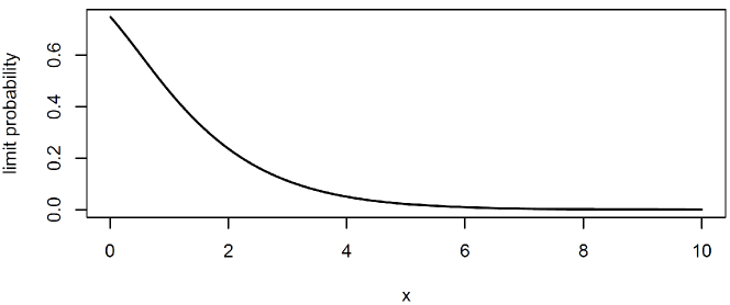
Figure 2: Shows $\lim_{\ell\to-\infty}\mathbb{P}^{x}(\tau(\ell)<\infty)$ as a function of $x$.

Assume that $r=s=1$, $\kappa=1$, $p=2/3$, $q=1/3$ and $\mu=\nu=1$. Then the limit in (39) is a decreasing function of $x$ as illustrated in Figure 2

Proof of Theorem 4.1.

Notation: In the proof we will write $f(\ell)=O(g(\ell))$ if there exists a constant $C$ such that $f(\ell)\sim Cg(\ell)$.

In the matrix $A(\ell)$ only $N^{3k}_{\Gamma_{j}}(\ell)$ (for $k=1,\ldots,r$ and $j=-s,\ldots,r-1$) depends on $\ell$. Exploring this dependence by applying the same technique as in the $x\to\infty$ case yields for $k=1,\ldots,r$ and $i=-s,\ldots,-1$ that

$$\lim_{\ell\to-\infty}\frac{N^{3k}_{\Gamma_{i}}(\ell)}{{\mathrm{e}}^{\ell\nu_{-i}}(-\ell)^{\frac{q\beta_{-i}\lambda}{\kappa}-1}} = \lim_{\ell\to-\infty}\frac{1}{{\mathrm{e}}^{\ell\nu_{-i}}(-\ell)^{\frac{q\beta_{-i}\lambda}{\kappa}-1}}\int_{\Gamma_{i,2}}\frac{\psi(z)}{z-\mu_{k}}{\mathrm{e}}^{-\ell z}\;{\mathrm{d}}z$$ (40)

$$= \frac{\psi_{\setminus\{-\nu_{-i}\}}(-\nu_{-i})}{-\nu_{-i}-\mu_{k}}\int_{\tilde{\Gamma}}z^{-\frac{q\beta_{-i}\lambda}{\kappa}}{\mathrm{e}}^{z}\;{\mathrm{d}}z$$

if $-\nu_{-i}$ is a zero for $\psi$. Here

$$\tilde{\Gamma}=\{(-1+i)t:0\leq t<\infty\}$$

and

$$\psi_{\setminus\{-\nu_{-i}\}}=z^{-1}\left(\prod_{k=1}^{r}(z-\mu_{k})^{-\frac{p\alpha_{k}\lambda}{\kappa}}\right)\left(\prod_{d=1,d\neq i}^{s}(z+\nu_{d})^{-\frac{q\beta_{d}\lambda}{\kappa}}\right)\,.$$

If $-\nu_{-i}$ is a singularity the result is

$$\lim_{\ell\to-\infty}\frac{N^{3k}_{\Gamma_{i}}(\ell)}{{\mathrm{e}}^{\ell\nu_{-i}}(-\ell)^{\frac{q\beta_{-i}\lambda}{\kappa}-1}}=\frac{\psi_{\setminus\{-\nu_{-i}\}}(-\nu_{-i})}{-\nu_{-i}-\mu_{k}}\int_{\tilde{\Gamma}_{a}}z^{-\frac{q\beta_{-i}\lambda}{\kappa}}{\mathrm{e}}^{z}\;{\mathrm{d}}z\,,$$ (41)

where

$$\tilde{\Gamma}_{a}=\{a+(1+i)t:-\infty<t\leq 0\}+\{a+(-1+i)t:0\leq t<\infty\}\,.$$

for any $a>0$. Furthermore

$$\lim_{\ell\to-\infty}N_{\Gamma_{0}}^{3k}(\ell)=\frac{\psi_{\setminus\{0\}}(0)}{-\mu_{k}}\int_{\tilde{\Gamma}_{a}}z^{-1}{\mathrm{e}}^{z}\,{\mathrm{d}}z\,.$$ (42)

Finally, the constants related to $\mu_{1},\ldots,\mu_{r}$ satisfy the following if $\mu_{i}$ is a zero

$$\lim_{\ell\to-\infty}\frac{N_{\Gamma_{i}}^{3i}(\ell)}{{\mathrm{e}}^{-\ell\mu_{i}}(-\ell)^{-\frac{p\alpha_{i}\lambda}{\kappa}}} = \psi_{\setminus\{\mu_{i}\}}(\mu_{i})\int_{\tilde{\Gamma}}z^{-\frac{p\alpha_{i}\lambda}{\kappa}-1}{\mathrm{e}}^{z}\;{\mathrm{d}}z$$ (43)

$$\lim_{\ell\to-\infty}\frac{N_{\Gamma_{i}}^{3k}(\ell)}{{\mathrm{e}}^{-\ell\mu_{i}}(-\ell)^{-\frac{p\alpha_{i}\lambda}{\kappa}-1}} = \frac{\psi_{\setminus\{\mu_{i}\}}(\mu_{i})}{\mu_{i}-\mu_{k}}\int_{\tilde{\Gamma}}z^{-\frac{p\alpha_{i}\lambda}{\kappa}}{\mathrm{e}}^{z}\;{\mathrm{d}}z\quad\textrm{ if }k\neq i$$ (44)

and if it is a singularity

$$\lim_{\ell\to-\infty}\frac{N_{\Gamma_{i}}^{3i}(\ell)}{{\mathrm{e}}^{-\ell\mu_{i}}(-\ell)^{-\frac{p\alpha_{i}\lambda}{\kappa}}} = \psi_{\setminus\{\mu_{i}\}}(\mu_{i})\int_{\tilde{\Gamma}_{a}}z^{-\frac{p\alpha_{i}\lambda}{\kappa}-1}{\mathrm{e}}^{z}\;{\mathrm{d}}z$$ (45)

$$\lim_{\ell\to-\infty}\frac{N_{\Gamma_{i}}^{3k}(\ell)}{{\mathrm{e}}^{-\ell\mu_{i}}(-\ell)^{-\frac{p\alpha_{i}\lambda}{\kappa}-1}} = \frac{\psi_{\setminus\{\mu_{i}\}}(\mu_{i})}{\mu_{i}-\mu_{k}}\int_{\tilde{\Gamma}_{a}}z^{-\frac{p\alpha_{i}\lambda}{\kappa}}{\mathrm{e}}^{z}\;{\mathrm{d}}z\quad\textrm{ if }k\neq i\,.$$ (46)

When calculating the determinant of $A(\ell)$ it is crucial that $N^{3k}_{\Gamma_{i}}(\ell)$ has the largest rate of growth when $k=i$. Furthermore, if $\mu_{i}$ is a singularity of an order in $(0,1)$ and $k\neq i$ then the limit integral for $N^{3k}_{\Gamma_{i}}(\ell)$ is zero while the integral in the limit of $N^{3i}_{\Gamma_{i}}(\ell)$ is not. Define the matrices

$$M=\left[\begin{array}[]{cccccc}M^{11}_{\Gamma_{1}}&\ldots&M^{11}_{\Gamma_{r}}&N^{11}_{\Gamma_{-s}}&\ldots&N^{11}_{\Gamma_{-1}}\\ \vdots&\ddots&\vdots&\vdots&\ddots&\vdots\\ M^{1r}_{\Gamma_{1}}&\ldots&M^{1r}_{\Gamma_{r}}&N^{1r}_{\Gamma_{-s}}&\ldots&N^{1r}_{\Gamma_{-1}}\\ -M^{21}_{\Gamma_{1}}&\ldots&-M^{21}_{\Gamma_{r}}&N^{21}_{\Gamma_{-s}}&\ldots&N^{21}_{\Gamma_{-1}}\\ \vdots&\ddots&\vdots&\vdots&\ddots&\vdots\\ -M^{2s}_{\Gamma_{1}}&\ldots&-M^{2s}_{\Gamma_{r}}&N^{2s}_{\Gamma_{-s}}&\ldots&N^{2s}_{\Gamma_{-1}}\end{array}\right]$$

and

$$N(\ell)=\left[\begin{array}[]{ccc}N_{\Gamma_{0}}^{31}(\ell)&\ldots&N_{\Gamma_{r-1}}^{31}(\ell)\\ \vdots&\ddots&\vdots\\ N_{\Gamma_{0}}^{3r}(\ell)&\ldots&N_{\Gamma_{r-1}}^{3r}(\ell)\\ \end{array}\right]\;.$$

The formulas (40) – (46) yield that $\det(A(\ell))\sim\big{(}\det(N(\ell))(-1)^{r+s+1}\det(M)\big{)}$ and by using that $N^{3i}_{\Gamma_{i}}(\ell)$ has the most rapid growth compared to $N^{3k}_{\Gamma_{i}}(\ell)$ when $k\neq i$, it is seen that

$$\det(N(\ell))\sim\left(N_{\Gamma_{0}}^{3r}(\ell)\prod_{i=1}^{r-1}N_{\Gamma_{i}}^{3i}(\ell)\right)$$

which implies that

$$\det(N(\ell))=O\left({\mathrm{e}}^{\ell\sum_{j=1}^{r-1}\mu_{j}}(-\ell)^{\sum_{j=1}^{r-1}\frac{p\alpha_{j}\lambda}{\kappa}}\right)\,.$$

Cramer’s Rule provides the constants $c_{1}(\ell),\ldots,c_{r}(\ell)$ and $b_{-s}(\ell),\ldots,b_{r-1}(\ell)$ in the equation system (38):

$$c_{1}(\ell)=\frac{\det(A_{1}(\ell))}{\det(A(\ell))}\,,$$

where

$$A_{1}(\ell)=\left[\begin{array}[]{ccccccc}\frac{1}{\mu_{1}}&0&\ldots&0&N^{31}_{\Gamma_{-s}}(\ell)&\ldots&N^{31}_{\Gamma_{r-1}}(\ell)\\ \vdots&\vdots&\ddots&\vdots&\vdots&\ddots&\vdots\\ \frac{1}{\mu_{r}}&0&\ldots&0&N^{3r}_{\Gamma_{-s}}(\ell)&\ldots&N^{3r}_{\Gamma_{r-1}}(\ell)\\ 0&M^{11}_{\Gamma_{2}}&\ldots&M^{11}_{\Gamma_{r}}&N^{11}_{\Gamma_{-s}}&\ldots&N^{11}_{\Gamma_{r-1}}\\ \vdots&\vdots&\ddots&\vdots&\vdots&\ddots&\vdots\\ 0&M^{1r}_{\Gamma_{2}}&\ldots&M^{1r}_{\Gamma_{r}}&N^{1r}_{\Gamma_{-s}}&\ldots&N^{1r}_{\Gamma_{r-1}}\\ 0&-M^{21}_{\Gamma_{2}}&\ldots&-M^{21}_{\Gamma_{r}}&N^{21}_{\Gamma_{-s}}&\ldots&N^{21}_{\Gamma_{r-1}}\\ \vdots&\vdots&\ddots&\vdots&\vdots&\ddots&\vdots\\ 0&-M^{2s}_{\Gamma_{2}}&\ldots&-M^{2s}_{\Gamma_{r}}&N^{2s}_{\Gamma_{-s}}&\ldots&N^{2s}_{\Gamma_{r-1}}\end{array}\right]\,,$$

and similarly for the remaining constants. It is seen that

$$\det(A_{i}(\ell))=O\left({\mathrm{e}}^{\ell\sum_{j=1}^{r-1}\mu_{j}}(-\ell)^{\sum_{j=1}^{r-1}\frac{p\alpha_{j}\lambda}{\kappa}}\right)$$

for $i=1,\ldots,r+s$ and therefore

$$c_{i}(\ell) = \frac{\det(A_{i}(\ell))}{\det(A(\ell))}=O(1)\qquad i=1,\ldots,r$$

$$b_{j}(\ell) = \frac{\det(A_{r+s+1+j}(\ell))}{\det(A(\ell))}=O(1)\qquad j=-s,\ldots,-1\,.$$

Furthermore,

$$\det(A_{r+s+1}(\ell)) \sim \left(\det(M)\times\frac{1}{\mu_{r}}\prod_{i=1}^{r-1}N_{\Gamma_{i}}^{3i}(\ell)\right)$$

$$\det(A_{r+s+1+j}(\ell)) \sim \left(\det(M)\times\frac{1}{\mu_{j}}N_{\Gamma_{0}}^{3r}(\ell)\prod_{i=1,i\neq j}^{r-1}N_{\Gamma_{i}}^{3i}(\ell)\right)\qquad j=1,\ldots,r-1$$

such that

$$b_{0}(\ell) = \frac{\det(A_{r+s+1}(\ell))}{\det(A(\ell))}\sim\left(\frac{1}{\mu_{r}}\frac{1}{N^{3r}_{\Gamma_{0}}(\ell)}\right)$$

$$b_{j}(\ell) = \frac{\det(A_{r+s+1+j}(\ell))}{\det(A(\ell))}\sim\left(\frac{1}{\mu_{j}}\frac{1}{N^{3j}_{\Gamma_{j}}(\ell)}\right)$$

$$\phantom{\frac{\det(A_{r+s+1+j}(\ell))}{\det(A(\ell))}}=O\left({\mathrm{e}}^{\ell\mu_{j}}(-\ell)^{\frac{p\alpha_{j}\lambda}{\kappa}}\right)\qquad j=1,\ldots,r-1\,.$$

The equivalent constants $\tilde{c}_{1}(\ell),\ldots,\tilde{c}_{r}(\ell)$ and $\tilde{b}_{-s+1}(\ell),\ldots,\tilde{b}_{r}(\ell)$ that belongs to the second partial eigenfunction solve an equation system similar to (38):

$$\left[\begin{array}[]{cccccc}0&\ldots&0&N^{31}_{\Gamma_{-s+1}}(\ell)&\ldots&N^{31}_{\Gamma_{r}}(\ell)\\ \vdots&\ddots&\vdots&\vdots&\ddots&\vdots\\ 0&\ldots&0&N^{3r}_{\Gamma_{-s+1}}(\ell)&\ldots&N^{3r}_{\Gamma_{r}}(\ell)\\ M^{11}_{\Gamma_{1}}&\ldots&M^{11}_{\Gamma_{r}}&N^{11}_{\Gamma_{-s+1}}&\ldots&N^{11}_{\Gamma_{r}}\\ \vdots&\ddots&\vdots&\vdots&\ddots&\vdots\\ M^{1r}_{\Gamma_{1}}&\ldots&M^{1r}_{\Gamma_{r}}&N^{1r}_{\Gamma_{-s+1}}&\ldots&N^{1r}_{\Gamma_{r}}\\ -M^{21}_{\Gamma_{1}}&\ldots&-M^{21}_{\Gamma_{r}}&N^{21}_{\Gamma_{-s+1}}&\ldots&N^{21}_{\Gamma_{r}}\\ \vdots&\ddots&\vdots&\vdots&\ddots&\vdots\\ -M^{2s}_{\Gamma_{1}}&\ldots&-M^{2s}_{\Gamma_{r}}&N^{2s}_{\Gamma_{-s+1}}&\ldots&N^{2s}_{\Gamma_{r}}\end{array}\right]\left[\begin{array}[]{c}\tilde{c}_{1}(\ell)\\ \vdots\\ \tilde{c}_{r}(\ell)\\ \tilde{b}_{-s+1}(\ell)\\ \vdots\\ \tilde{b}_{r}(\ell)\end{array}\right]=\left[\begin{array}[]{c}\frac{1}{\mu_{1}}\\ \vdots\\ \frac{1}{\mu_{r}}\\ 0\\ \vdots\\ 0\end{array}\right]\,,$$ (47)

where the integration contour $\Gamma_{-s}$ is replaced by $\Gamma_{r}$ in order to obtain a new and independent partial eigenfunction. It is similarly shown that the constants have the following asymptotics as functions of $\ell$

$$\tilde{c}_{i}(\ell) = O\left(\frac{1}{\mu_{1}}\frac{1}{N^{31}_{\Gamma_{1}}(\ell)}\right)=O\left({\mathrm{e}}^{-\ell\mu_{1}}(-\ell)^{\frac{p\alpha_{1}\lambda}{\kappa}}\right)\qquad i=-s,\ldots,-1$$

$$\tilde{b}_{j}(\ell) = O\left(\frac{1}{\mu_{1}}\frac{1}{N^{31}_{\Gamma_{1}}}(\ell)\right)=O\left({\mathrm{e}}^{-\ell\mu_{1}}(-\ell)^{\frac{p\alpha_{1}\lambda}{\kappa}}\right)\qquad j=-s+1,\ldots,0$$

$$\tilde{b}_{j}(\ell) \sim \left(\frac{1}{\mu_{j}}\frac{1}{N^{3j}_{\Gamma_{j}}}(\ell)\right)=O\left({\mathrm{e}}^{-\ell\mu_{j}}(-\ell)^{\frac{p\alpha_{j}\lambda}{\kappa}}\right)\qquad j=1,\ldots,r\,.$$

The asymptotic behaviour of the $f_{\Gamma_{j,2}}^{2}$ functions is of interest as well. Similar to the previous analysis it is seen that for $j=-s,\ldots,-1$ is

$$\lim_{\ell\to-\infty}\frac{f^{2}_{\Gamma_{j,2}}(\ell)}{{\mathrm{e}}^{\ell\nu_{-j}}(-\ell)^{\frac{q\beta_{j}\lambda}{\kappa}-1}}=\psi_{\setminus\{-\nu_{-j}\}}(-\nu_{-j})\int_{\tilde{\Gamma}_{a}}z^{-\frac{q\beta_{j}\lambda}{\kappa}}{\mathrm{e}}^{z}\;{\mathrm{d}}z\,,\textrm{ if $\nu_{-j}$ is a singularity}$$

$$\lim_{\ell\to-\infty}\frac{f^{2}_{\Gamma_{j,2}}(\ell)}{{\mathrm{e}}^{\ell\nu_{-j}}(-\ell)^{\frac{q\beta_{j}\lambda}{\kappa}-1}}=\psi_{\setminus\{-\nu_{-j}\}}(-\nu_{-j})\int_{\tilde{\Gamma}}z^{-\frac{q\beta_{j}\lambda}{\kappa}}{\mathrm{e}}^{z}\;{\mathrm{d}}z\,,\textrm{ if $\nu_{-j}$ is a root}\,.$$

For $j=0$ is

$$\lim_{j\to-\infty}f^{2}_{\Gamma_{0,2}}(\ell)=\psi_{\setminus\{0\}}(0)\int_{\tilde{\Gamma}_{a}}z^{-1}{\mathrm{e}}^{z}\;{\mathrm{d}}z\,,$$

and for $j=1,\ldots,r$ is

$$\lim_{\ell\to-\infty}\frac{f^{2}_{\Gamma_{j,2}}(\ell)}{{\mathrm{e}}^{-\ell\mu_{j}}(-\ell)^{\frac{p\alpha_{j}\lambda}{\kappa}-1}} = \psi_{\setminus\{\mu_{j}\}}(\mu_{j})\int_{\tilde{\Gamma}_{a}}z^{-\frac{p\alpha_{j}\lambda}{\kappa}}{\mathrm{e}}^{z}\;{\mathrm{d}}z\,,\quad\textrm{if $\mu_{j}$ is a singularity}$$

$$\lim_{\ell\to-\infty}\frac{f^{2}_{\Gamma_{j,2}}(\ell)}{{\mathrm{e}}^{-\ell\mu_{j}}(-\ell)^{\frac{p\alpha_{j}\lambda}{\kappa}-1}} = \psi_{\setminus\{\mu_{j}\}}(\mu_{j})\int_{\tilde{\Gamma}}z^{-\frac{q\alpha_{j}\lambda}{\kappa}}{\mathrm{e}}^{z}\;{\mathrm{d}}z\,,\quad\textrm{if $\mu_{j}$ is a root}\,.$$

By comparing these results with the asymptotics for the constants $c_{i}(\ell)$, $\tilde{c}_{i}(\ell)$, $b_{j}(\ell)$ and $\tilde{b}_{j}(\ell)$ it is seen that

• $b_{j}(\ell)f^{2}_{\Gamma_{j,2}}(\ell)$ tends to zero exponentially fast as $\ell\to-\infty$ for $j=-s,\ldots,-1$

• $\tilde{b}_{j}(\ell)f^{2}_{\Gamma_{j,2}}(\ell)$ tends to zero exponentially fast as $\ell\to-\infty$ for $j=-s+1,\ldots,0$

• $b_{j}(\ell)f^{2}_{\Gamma_{j,2}}(\ell)=O\left(\frac{1}{-\ell}\right)$ for $\ell\to-\infty$ when $j=1,\ldots,r-1$

• $\tilde{b}_{j}(\ell)f^{2}_{\Gamma_{j,2}}(\ell)=O\left(\frac{1}{-\ell}\right)$ for $\ell\to-\infty$ when $j=1,\ldots,r$ .

Finally, the non–zero limit of $b_{0}(\ell)f^{2}_{\Gamma_{0,2}}(\ell)$ when $\ell\to-\infty$ is

$$\lim_{\ell\to-\infty}b_{0}(\ell)f^{2}_{\Gamma_{0,2}}(\ell) = \lim_{\ell\to-\infty}\frac{1}{\mu_{r}}\frac{1}{N^{3r}_{\Gamma_{0}}(\ell)}f^{2}_{\Gamma_{0,2}}(\ell)$$

$$= \frac{1}{\mu_{r}}\frac{\psi_{\setminus\{0\}}(0)\int_{\tilde{\Gamma}_{a}}z^{-1}{\mathrm{e}}^{z}\;{\mathrm{d}}z}{\frac{\psi_{\setminus\{0\}}(0)}{-\mu_{r}}\int_{\tilde{\Gamma}_{a}}z^{-1}{\mathrm{e}}^{z}\,{\mathrm{d}}z}$$

$$= -1\,.$$

Hence it has been shown that

$$\lim_{\ell\to-\infty}f_{1}(\ell) = \lim_{\ell\to-\infty}\sum_{j=-s}^{r-1}b_{j}(\ell)f_{\Gamma_{j,2}}^{2}(\ell)=-1$$

$$\lim_{\ell\to-\infty}f_{2}(\ell) = \lim_{\ell\to-\infty}\sum_{j=-s+1}^{r}\tilde{b}_{j}(\ell)f_{\Gamma_{j,2}}^{2}(\ell)=0\,.$$

Furthermore it is shown that all $\tilde{c}_{i}(\ell)$ decrease to zero so

$$\lim_{\ell\to-\infty}f_{2}(x)=\lim_{t\to-\infty}\sum_{i=1}^{r}\tilde{c}_{i}(\ell)f^{1}_{\Gamma_{i,1}}(x)=0$$

and since all $c_{i}$ has a non–zero limit, then $\lim_{\ell\to-\infty}f_{1}(x)$ is well–defined and non–zero. Therefore

$$\lim_{\ell\to-\infty}\mathbb{P}^{x}(\tau<\infty)$$

$$=\lim_{\ell\to-\infty}f_{1}(x)\frac{1-f_{2}(\ell)}{f_{1}(\ell)-f_{2}(\ell)}+f_{2}(x)\frac{f_{1}(\ell)-1}{f_{1}(\ell)-f_{2}(\ell)}=-\lim_{\ell\to-\infty}f_{1}(x)\,.$$

∎

The asymptotic expression for $c_{i}(\ell)$ can found to be

$$c_{i}(\ell)\sim\left((-1)^{r+s+1-i}\frac{det(M_{i})}{det(M)}\frac{1}{\mu_{r}N^{3r}_{\Gamma_{0}}(\ell)}\right)\,,$$

where

$$M_{i}=\left[\begin{array}[]{ccccccccc}M^{11}_{\Gamma_{1}}&\ldots&M^{11}_{\Gamma_{i-1}}&M^{11}_{\Gamma_{i+1}}&\ldots&M^{11}_{\Gamma_{r}}&N^{11}_{\Gamma_{-s}}&\ldots&N^{11}_{\Gamma_{0}}\\ \vdots&\ddots&\vdots&\vdots&\ddots&\vdots&\vdots&\ddots&\vdots\\ M^{1r}_{\Gamma_{1}}&\ldots&M^{1r}_{\Gamma_{i-1}}&M^{1r}_{\Gamma_{i+1}}&\ldots&M^{1r}_{\Gamma_{r}}&N^{1r}_{\Gamma_{-s}}&\ldots&N^{1r}_{\Gamma_{0}}\\ -M^{21}_{\Gamma_{1}}&\ldots&-M^{21}_{\Gamma_{i-1}}&-M^{21}_{\Gamma_{i+1}}&\ldots&-M^{21}_{\Gamma_{r}}&N^{21}_{\Gamma_{-s}}&\ldots&N^{21}_{\Gamma_{0}}\\ \vdots&\ddots&\vdots&\vdots&\ddots&\vdots&\vdots&\ddots&\vdots\\ -M^{2s}_{\Gamma_{1}}&\ldots&-M^{2s}_{\Gamma_{i-1}}&-M^{2s}_{\Gamma_{i+1}}&\ldots&-M^{2s}_{\Gamma_{r}}&N^{2s}_{\Gamma_{-s}}&\ldots&N^{2s}_{\Gamma_{0}}\end{array}\right]\;.$$

Hence we have

Corollary 4.1.

For $i=1,\ldots,r$ it holds that

$$\lim_{\ell\to-\infty}c_{i}(\ell) = (-1)^{r+s+1-i}\frac{\det(M_{i})}{\det(M)}\frac{1}{\mu_{r}}\left(\frac{\psi_{\setminus\{0\}}(0)}{-\mu_{k}}\int_{\tilde{\Gamma}_{a}}z^{-1}{\mathrm{e}}^{z}\,{\mathrm{d}}z\right)^{-1}$$

$$= (-1)^{r+s-i}\frac{\det(M_{i})}{\det(M)}\left(\psi_{\setminus\{0\}}(0)\int_{\tilde{\Gamma}_{a}}z^{-1}{\mathrm{e}}^{z}\,{\mathrm{d}}z\right)^{-1}\,.$$

4.2 Negative drift and the undershoot

Consider the negative drift case, $\kappa<0$, where the ruin probability is 1. This situation is particularly simple because only one partial eigenfunction, $f$, is needed, since crossing $\ell$ through continuity is not possible. The Laplace transform of the undershoot is therefore expressed by the simple formula

$$\mathbb{E}^{x}[{\mathrm{e}}^{-\zeta Z}]=f(x)\,.$$

Since $\psi$ satisfies that $|\psi(z)|=O(|z|^{-1-\tfrac{\lambda}{\kappa}})$, the negative $\kappa$ makes infinite integration contours impossible. We shall apply Theorem 2.1 and choose finite integration contours as described in [10, Section 5]. However, in [10] the contours are suggested to be half–circles and circles, but that choice makes the calculations of our prblem too complicated. Thus we will use line segments instead. Note that $\mu_{1}$ is always a zero for $\psi$. For each $i=2,\ldots,r$ define:
If $\mu_{i}$ is a zero define $\Gamma_{i}$ as

$$\{\mu_{i}+(-1-i)t\;:\;0\leq t\leq\frac{\mu_{i}-\mu_{1}}{2}\}$$

$$\phantom{=}\cup\{\mu_{i}-i(\mu_{i}-\mu_{1})+(-1+i)t\;:\;\frac{\mu_{i}-\mu_{1}}{2}\leq t\leq\mu_{i}-\mu_{1}\}\,.$$

If $\mu_{i}$ is a singularity define $\Gamma_{i}$ as

$$\{\mu_{i}+\tfrac{a}{-\ell}+i(\mu_{i}+\tfrac{a}{-\ell}-\mu_{1})+(1+i)t:-(\mu_{i}+\tfrac{a}{-\ell}-\mu_{1})\leq t\leq-\frac{\mu_{i}+\frac{a}{-\ell}-\mu_{1}}{2}\}$$

$$\phantom{=}\cup\{\mu_{i}+\tfrac{a}{-\ell}+(1-i)t:-\frac{\mu_{i}+\frac{a}{-\ell}-\mu_{1}}{2}\leq t\leq 0\}$$

$$\phantom{=}\cup\{\mu_{i}+\tfrac{a}{-\ell}+(-1-i)t:\frac{\mu_{i}+\frac{a}{-\ell}-\mu_{1}}{2}\leq t\leq 0\}$$

$$\phantom{=}\cup\{\mu_{i}-\tfrac{a}{-\ell}+i(\mu_{i}+\tfrac{a}{-\ell}-\mu_{1})+(-1+i)t:\frac{\mu_{i}+\frac{a}{-\ell}-\mu_{1}}{2}\leq t\leq\mu_{i}+\tfrac{a}{-\ell}-\mu_{1}\}\,.$$

A rough sketch of the two contours can be seen on Figure 3.

Figure 3: The choice of contours in the negative drift case .

The partial eigenfunction $f$ is defined by

$$f(y)=\sum_{i=2}^{r}c_{i}f_{\Gamma_{i}}(y)+Uf^{*}(y)+f_{0}(y)\,,$$ (48)

where $f^{*}(y)=1_{[\ell;\infty[}(y)$, and the parameters $c_{2},\ldots,c_{r}$ and $U$ are the solutions of the equation

$$\left[\begin{array}[]{cccc}-\frac{1}{\mu_{1}}(\ell)&M_{\Gamma_{2}}^{1}(\ell)&\cdots&M^{1}_{\Gamma_{r}}(\ell)\\ -\frac{1}{\mu_{2}}(\ell)&M_{\Gamma_{2}}^{2}(\ell)&\cdots&M^{2}_{\Gamma_{r}}(\ell)\\ \vdots&\vdots&\ddots&\vdots\\ -\frac{1}{\mu_{r}}(\ell)&M_{\Gamma_{2}}^{r}(\ell)&\cdots&M^{r}_{\Gamma_{r}}(\ell)\end{array}\right]\left[\begin{array}[]{c}U\\ c_{2}\\ \vdots\\ c_{r}\end{array}\right]=\left[\begin{array}[]{c}-\frac{1}{\mu_{1}+\zeta}\\ \vdots\\ -\frac{1}{\mu_{r}+\zeta}\end{array}\right]$$ (49)

where we shall denote the first matrix by $B(\ell)$ and the constants $M_{\Gamma_{i}}^{k}(\ell)$ are given as

$$M_{\Gamma_{i}}^{k}(\ell)=\int_{\Gamma_{i}}\frac{\psi(z)}{z-\mu_{k}}{\mathrm{e}}^{-\ell z}\,{\mathrm{d}}z$$ (50)

for $i=2,\ldots,r$ and $k=1,\ldots,r$. To explore the asymptotic behaviour of $U,c_{2},\ldots,c_{r}$ and through that the behaviour of $f$, it is necessary to study the constants in (50).

The following result states that the limit of the undershoot is a simple exponential distribution with parameter $\mu_{1}$ from the dominating part of the downward jumps.

Theorem 4.2.

For all $\zeta\geq 0$ it holds that

$$\lim_{\ell\to-\infty}\mathbb{E}^{x}[{\mathrm{e}}^{-\zeta Z}]=\frac{\mu_{1}}{\mu_{1}+\zeta}\,.$$

Proof.

First the behaviour of the constants $M_{\Gamma_{i}}^{k}(\ell)$ when $\ell\to-\infty$ is explored. When $\mu_{i}$ is a zero (for some $i=2,\ldots,r$) and $i\neq k$ the constant can be written as

$$M_{\Gamma_{i}}^{k}(\ell)=\int_{0}^{\frac{\mu_{i}-\mu_{1}}{2}}(-1-i)\frac{\psi(\mu_{i}+(-1-i)t)}{\mu_{i}+(-1-i)t-\mu_{k}}{\mathrm{e}}^{-\ell(\mu_{i}+(-1-i)t)}\,{\mathrm{d}}t$$ (51)

$$+\int_{\frac{\mu_{i}-\mu_{1}}{2}}^{\mu_{i}-\mu_{1}}(-1+i)\frac{\psi(\mu_{i}-i(\mu_{i}-\mu_{1})+(-1+i)t)}{\mu_{i}-i(\mu_{i}-\mu_{1})+(-1+i)t-\mu_{k}}{\mathrm{e}}^{-\ell(\mu_{i}-i(\mu_{i}-\mu_{1})+(-1+i)t)}\,{\mathrm{d}}t\,.$$

Rewriting the expression and applying the usual substitution $s=-\ell t$ to the first part in (51) yields

$$M_{\Gamma_{i}}^{k}(\ell)={\mathrm{e}}^{-\ell\mu_{i}}(-\ell)^{\frac{p\lambda\alpha_{i}}{\kappa}-1} \int_{0}^{(-\ell)\frac{\mu_{i}-\mu_{1}}{2}}(-1-i)\frac{\psi_{\setminus\{\mu_{i}\}}(\mu_{i}+(-1-i)\tfrac{s}{-\ell})}{\mu_{i}+(-1-i)\tfrac{s}{-\ell}-\mu_{k}}\times$$

$$((-1-i)s)^{-\frac{p\lambda\alpha_{i}}{\kappa}}{\mathrm{e}}^{s(-1-i)}\,{\mathrm{d}}s\,.$$

Hence, by dominated convergence it is seen that the integral in the last line has the limit

$$\frac{\psi_{\setminus\{\mu_{i}\}}(\mu_{i})}{\mu_{i}-\mu_{k}}\int_{0}^{\infty}(-1-i)((-1-i)s)^{-\frac{p\lambda\alpha_{i}}{\kappa}}{\mathrm{e}}^{s(-1-i)}\,{\mathrm{d}}s$$

$$= \frac{\psi_{\setminus\{\mu_{i}\}}(\mu_{i})}{\mu_{i}-\mu_{k}}\int_{-\Gamma}z^{-\frac{p\lambda\alpha_{i}}{\kappa}}{\mathrm{e}}^{z}\,{\mathrm{d}}z\,,$$

where

$$-\Gamma=\{(-1-i)t:0\leq t<\infty\}\,.$$

Now remains to discuss the asymptotics of the second part in (51). Substituting $s=-\ell(t-(\mu_{i}-\mu_{1}))$ the expression equals

$${\mathrm{e}}^{-\ell(\frac{\mu_{1}+\mu_{i}}{2}-i\frac{\mu_{i}-\mu_{1}}{2})}(-\ell)^{-1}$$

$$\times\int_{0}^{(-\ell)\frac{\mu_{i}-\mu_{1}}{2}}(-1+i)\psi\left(\frac{\mu_{1}+\mu_{i}}{2}-i\frac{\mu_{i}-\mu_{1}}{2}+(-1+i)\tfrac{s}{-\ell}\right){\mathrm{e}}^{s(-1+i)}\,{\mathrm{d}}s\,.$$

The integral has the following limit for $\ell\to-\infty$

$$\psi\left(\frac{\mu_{1}+\mu_{i}}{2}-i\frac{\mu_{i}-\mu_{1}}{2}\right)\int_{\tilde{\Gamma}}{\mathrm{e}}^{z}\,{\mathrm{d}}z$$

by dominated convergence, where $\tilde{\Gamma}=\{(-1+i)t:0\leq t<\infty\}$. Since the first part grows with a larger rate than the last part is

$$\lim_{\ell\to-\infty}\frac{M_{\Gamma_{i}}^{k}(\ell)}{{\mathrm{e}}^{-\ell\mu_{i}}(-\ell)^{-\frac{p\lambda\alpha_{i}}{\kappa}-1}}=\frac{\psi_{\setminus\{\mu_{i}\}}(\mu_{i})}{\mu_{i}-\mu_{k}}\int_{-\Gamma}z^{-\frac{p\lambda\alpha_{i}}{\kappa}}{\mathrm{e}}^{z}\,{\mathrm{d}}z\,.$$ (52)

A similar result is found in the case where $i=k$:

$$\lim_{\ell\to-\infty}\frac{M_{\Gamma_{i}}^{k}(\ell)}{{\mathrm{e}}^{-\ell\mu_{i}}(-\ell)^{-\frac{p\lambda\alpha_{i}}{\kappa}}}=\psi_{\setminus\{\mu_{i}\}}(\mu_{i})\int_{-\Gamma}z^{-\frac{p\lambda\alpha_{i}}{\kappa}-1}{\mathrm{e}}^{z}\,{\mathrm{d}}z\,.$$ (53)

The same substitution technique yields results in the cases where $\mu_{i}$ are singularities for $\psi$. That gives

$$\lim_{\ell\to-\infty}\frac{M_{\Gamma_{i}}^{k}(\ell)}{{\mathrm{e}}^{-\ell\mu_{i}}(-\ell)^{-\frac{p\lambda\alpha_{i}}{\kappa}-1}}=\frac{\psi_{\setminus\{\mu_{i}\}}(\mu_{i})}{\mu_{i}-\mu_{k}}\int_{-\Gamma_{a}}z^{-\frac{p\lambda\alpha_{i}}{\kappa}}{\mathrm{e}}^{z}\,{\mathrm{d}}z$$ (54)

if $i\neq k$ and

$$\lim_{\ell\to-\infty}\frac{M_{\Gamma_{i}}^{k}(\ell)}{{\mathrm{e}}^{-\ell\mu_{i}}(-\ell)^{-\frac{p\lambda\alpha_{i}}{\kappa}}}=\psi_{\setminus\{\mu_{i}\}}(\mu_{i})\int_{-\Gamma_{a}}z^{-\frac{p\lambda\alpha_{i}}{\kappa}-1}{\mathrm{e}}^{z}\,{\mathrm{d}}z$$ (55)

when $i=k$. Here

$$-\Gamma_{a}=\{a+(1-i)t:-\infty<t\leq 0\}\cup\{a+(-1-i)t:0\leq t<\infty\}\,.$$

sing (52)-(55) we obtain the following asymptotic behaviour of the determinant of the matrix $B(\ell)$,

$$\det(B(\ell))\sim\left(-\frac{1}{\mu_{1}}\prod_{i=2}^{r}M^{i}_{\Gamma_{i}}(\ell)\right)\,.$$ (56)

Let $B_{i}$ denote $B$ with the $i$th column replaced by the vector $[-\frac{1}{\mu_{1}+\zeta},\ldots,-\frac{1}{\mu_{r}+\zeta}]^{T}$, then

$$\det(B_{1}(\ell)) \sim \left(-\frac{1}{\mu_{1}+\zeta}\prod_{i=2}^{r}M^{i}_{\Gamma_{i}}(\ell)\right)$$ (57)

$$\det(B_{i}(\ell)) \sim \left(\Big{(}\frac{-1}{\mu_{1}}\frac{1}{\mu_{i}+\zeta}-\frac{-1}{\mu_{i}}\frac{1}{\mu_{1}+\zeta}\Big{)}\prod_{j\in\{2,\ldots,r\},j=i}M^{j}_{\Gamma_{j}}(\ell)\right)\,.$$ (58)

The solutions of equation (49) are obtained from Cramer’s rule, and the asymptotic behaviour is determined from the results (56)-(58). This yields

$$U(\ell) = \frac{\det(B_{1}(\ell))}{\det(B(\ell))}\sim\left(\frac{\frac{-1}{\mu_{1}+\zeta}}{\frac{-1}{\mu_{1}}}\right)=\frac{\mu_{1}}{\mu_{1}+\zeta}$$

$$c_{i}(\ell) = \frac{\det(B_{i}(\ell))}{\det(B(\ell))}\sim\left(\frac{\frac{-1}{\mu_{1}}\frac{1}{\mu_{i}+\zeta}-\frac{-1}{\mu_{i}}\frac{1}{\mu_{1}+\zeta}}{\frac{-1}{\mu_{1}}}\frac{1}{M_{\Gamma_{i}}^{i}(\ell)}\right)$$

with $i=2,\ldots,r$. Since all $M_{\Gamma_{i}}^{i}(\ell)$ are growing exponentially fast the asymptotics for $f$ defined in (48) are easily determined, as well as the limit of the Laplace transform for the undershoot,

$$\lim_{\ell\to-\infty}\mathbb{E}^{x}[{\mathrm{e}}^{-\zeta Z}] = \lim_{\ell\to-\infty}\left(\sum_{i=2}^{r}c_{i}(\ell)f_{\Gamma_{i}}(x)+U(\ell)f^{*}(x)\right)$$

$$= \lim_{\ell\to-\infty}U(\ell)\cdot 1$$

$$= \frac{\mu_{1}}{\mu_{1}+\zeta}\,.$$

∎

References

• [1] Asmussen, S. (2000). Ruin Probabilities World Scientific, Singapore.
• [2] Borovkov, K and Novikov, A. (2008). On exit times of Lévy–driven Ornstein–Uhlenbeck processes. Stat. and Prob. letters 78, 1517–1525.
• [3] Chen, Y. and Ng, K.W. (2007). The ruin probability of the renewal model with constant interest force and negatively dependent heavy–tailed claims. Ins., Math. & Eco. 40, 415–423.
• [4] Embrechts, P. and Schmidli, H. (1994). Ruin estimation for a general insurance risk model. Adv. Appl. Prob. 26, 402–422.
• [5] Gaier, J. and Grandits, P. (2004). Ruin probabilities and investment under interest force in the presence of regularly varying tails. Scand. Act. Journ. 256–278.
• [6] Grandits, P. (2004). A Karameta–type theorem and ruin probabilities for an insurer investing proportionally in the stock market. Insurance, Mathematics & Economics 34, 297–305.
• [7] Jacobsen, M. (2003). Martingales and the distribution of the time to ruin. Stoch. Proc. Appl. 107, 29-51.
• [8] Jacobsen, M. (2005). The time to ruin for a class of Markov additive risk processes with two–sided jumps. Adv. Appl. Probab. 38, 963-992.
• [9] Jacobsen, M. (2012). The time to ruin in some additive risk models with random premium rate. Journ. Appl. Probab. 49, 915-938.
• [10] Jacobsen, M and Jensen, A.T. (2007). Exit times for a class of piecewise exponential Markov processes with two–sided jumps. Stoch. Proc. Appl. 117, 1330–1356.
• [11] Jiang, T. and Yan, H-F. (2006). The finite–time ruin probability for the jump–diffusion model with constant interest force Acta mathematicae Applicatae Sinica, 22, 171–176.
• [12] Novikov, A., Melchers, R.E., Shinjikashvili, E. and Kordzakhia, N. (2005). First passage time of filtered Process with exponential shape function. Probabilistic Engineering Mechanics 20, 33-44.
• [13] Paulsen, J and Gjessing, H. K. (1997). Ruin theory with stochastic return on investments. emphAdv. Appl. Prob. 29, 965-985.
• [14] Schmidli, H. (1994). Risk theory in an economic environment and Markov processes Mitteiungen der Vereinigung der Versicherungsmatematiker 51–70.