Finite Element Method for a space-fractional anti-diffusive equation

Abstract.

The numerical solution of a nonlinear and space-fractional anti-diffusive equation used to model dune morphodynamics is considered. Spatial discretization is effected using a finite element method whereas the Crank-Nicolson scheme is used for temporal discretization. The fully discrete scheme is analyzed to determine stability condition and also to obtain error estimates for the approximate solution. Numerical examples are presented to illustrate convergence results.

1. Introduction

We consider the Fowler equation [7]

(1.1) $$\partial_{t}u(t,x)+\partial_{x}\left(\frac{u^{2}}{2}\right)(t,x)-\partial_{xx}u(t,x)+\mathcal{I}[u](t,x)=0,\quad x\in{\mathbf{R}},t>0,$$

where $\mathcal{I}$ is a nonlocal operator defined as follows: for any Schwartz function $\varphi\in\mathcal{S}(\mathbf{R})$ and any $x\in{\mathbf{R}}$,

(1.2) $$\mathcal{I}[\varphi](x):=\int_{0}^{+\infty}|\xi|^{-\frac{1}{3}}\varphi^{\prime\prime}(x-\xi)\,d\xi.$$

The Fowler equation was introduced to model the formation and dynamics of sand structures such as dunes and ripples [7]. This equation is valid for a river flow over an erodible bottom $u(t,x)$ with slow variation. Its originality resides in the nonlocal term, wich is anti-dissipative, and can been seen as a fractional Laplacian of order $4/3$. Indeed, it has been proved in [2] that

$$\mathcal{F}(\mathcal{I}[\varphi])(\xi)=-4\pi^{2}\Gamma(\frac{2}{3})\left(\frac{1}{2}-i\mbox{sgn}(\xi)\frac{\sqrt{3}}{2}\right)|\xi|^{4/3}\mathcal{F}(\varphi)(\xi),$$

where $\Gamma$ is the gamma function and $\mathcal{F}$ denotes the Fourier transform.
Therefore, this term has a deregularizing effect on the initial data but the instabilities produced by the nonlocal term are controled by the diffusion operator $-\partial_{x}^{2}$ which ensures the existence and the uniqueness of a smooth solution. We then always assume that there exists a sufficiently regular solution $u(t,x)$.
The use of Fourier transform is a natural way to study this equation but it also can be useful to consider the following formula:
for all $r>0$ and all $\varphi\in\mathcal{S}({\mathbf{R}})$,

(1.3) $$\mathcal{I}[\varphi](x) = \mathcal{I}_{1}[\varphi](x)+\mathcal{I}_{2}[\varphi](x),$$

with

$$\mathcal{I}_{1}[\varphi](x)=\int_{0}^{r}|\xi|^{-1/3}\varphi^{\prime\prime}(x-\xi)\,d\xi$$

and

$$\mathcal{I}_{2}[\varphi](x) = -\frac{1}{3}\int_{r}^{\infty}|\xi|^{-4/3}\varphi^{\prime}(x-\xi)\,d\xi+\varphi^{\prime}(x-r)r^{-1/3}.$$

Several numerical approaches have been suggested in the literature to overcome the equations with nonlocal operator. Droniou used a general class of difference methods for fractional conservation laws [5], Zheng and Roop proposed a finite element method to solve a space-fractional advection equations [14], [11]. Liu proposed a numerical solution for the fractional fokkerplanck equation [9]. Meerschaert studied finite difference approximations of fractional advection dispersion flow equation [10]. Fix presented a least squares finite-element approximations of a fractional order differential equation [6]. Xu applied the discontinuous Galerkin method to fractional convection diffusion equations with a fractional Laplacian of order $\lambda\in(1,2)$ [13] and, recently Guan investigated stabitlity and error estimates for $\theta$ schemes for finite element discretization of the space-time fractional diffusion equations [8].
To solve the Fowler equation (1.1) some numerical experiments have been performed using mainly finite difference method and split-step Fourier method [3].
We propose here to use the standard Galerkin method for the space approximation and a Crank-Nicolson scheme for the time discretization, which is a more simple way to improve approximations and to model complex geometries.
For $T>0,L>0$, we seek a function $u$ defined on ${\mathbf{R}}\times[0,T]$, 2L-periodic in the second variable and satisfying

(1.4) $$\left\{\begin{aligned} &\partial_{t}u(t,x)+\partial_{x}\left(\frac{u^{2}}{2}-\partial_{x}u+\mathcal{J}[u]\right)(t,x)=0,\quad x\in{\mathbf{R}},t\in(0,T),\\ &u(0,x)=u_{0}(x),\quad x\in{\mathbf{R}},\end{aligned}\right.$$

where $u_{0}$ is a given 2L-periodic function and

(1.5) $$\mathcal{J}[\varphi](x):=\int_{0}^{+\infty}|\xi|^{-\frac{1}{3}}\varphi^{\prime}(x-\xi)\,d\xi.\\$$

To prove the convergence of the numerical scheme we use the standard material on the finite element method for parabolic problems [12]. However, the analysis of the variational solution to the Fowler equation is more complicated than the usual parabolic equations because the fractional differential operator is not local and is anti-diffusive.
In this paper we analyze the discretization of (1.4) by a Crank-Nicolson method in time combined with the standard Garlerkin-finite element method in space. Our main result consists in prove the following error estimate:

$$||u(t^{n},\cdot)-U^{n}||\leq C(\Delta t^{2}+h^{k}),$$

where $k$ is the optimal spatial rate of convergence in $L^{2}$, $\Delta t=T/N$ is the time step, $t^{n}=n\Delta t,n=0,\cdots,N$ and $h$ is the spatial discretization. $U^{0},\cdots,U^{N}$ are the approximations of the solutions at different times.
We also prove that our numerical scheme is stable if the following condition is satisfied:

$$C_{1}\frac{\Delta t}{h^{2}}+C_{2}\frac{\Delta t}{h^{4/3}}\leq 1,$$

where $C_{1},C_{2}$ are two positive constants independent of $\Delta t$ and $h$.

It is clear that our analysis can easily be extended to the case where the nonlocal term $\mathcal{I}$ is replaced with a Fourier multiplier homogeneous of degree $\lambda\in]1,2[$ and not only $\lambda=4/3$ . It also can replaced with the Riemann-Liouvillle integral. Indeed, for causal functions, our nonlocal term is, up to a multplicative constant, a Riemann-Liouville operator defined as follows:

$$\frac{d^{4/3}\varphi}{dx}(x)=\frac{1}{\Gamma(2/3)}\int_{0}^{+\infty}|\xi|^{-1/3}\varphi^{\prime\prime}(x-\xi)\,d\xi.\\$$

The rest of this paper is construct as follows. In the next section we give the preliminary knowledge regarding the fractional operator and some technical Lemmas. We also introduce a projection operator and derive some error estimates which will play an important role in the sequel. The error estimate for the Galerkin-finite element method to solve the problem (1.4) is studied in Section 3. In section 4, we derive error estimates and prove existence and uniqueness of the fully discrete approximations. We also give a stability result.
We finally perform some numerical experiments to confirm the theoretical results in section 5.

1.1. Notations

• We denote by $C(c_{1},c_{2},...)$ a generic positive constant, strictly positive, which depends on parameters $c_{1},c_{2},\cdots$

• For $m\in{\mathbf{N}}$, let $H^{m}_{per}$ be the periodic Sobolev space of order $m$, consisting of the $2L-$periodic elements of $H^{m}_{loc}({\mathbf{R}}).$ We denote by $||\cdot||_{m}$ the norm over a period in $H^{m}_{per}$, by $||\cdot||$ the norm in $L^{2}(-L,L)$, and by $(\cdot,\cdot)$ the inner product in $L^{2}(-L,L)$.

• We denote by $C_{n}(\varphi)$ the Fourier coefficient of $\varphi$ defined by: for all $n\in\mathbb{Z}$

  $$C_{n}(\varphi)=\frac{1}{2L}\int_{-L}^{L}\varphi(x)e^{-i\frac{n}{L}x}\,dx$$

2. Preliminaries

In this section, we give the variational formulation of the problem (1.4) and we introduce a projection operator. We derive some estimates wich will be useful in the next sections.

We shall discretize (1.4) in space by the Galerkin method. To this effect, let $-L=x_{0}<x_{1}<\cdots<x_{N}=L$ be a partition of $[-L,L]$ and $h:=\max_{j}(x_{j+1}-x_{j})$.
For integer $r\geq 2$, let $\mathcal{S}_{h}^{r}$ denote a space of continuously differentiable, 2L-periodic functions of degree $r-1$ in which approximations to the solution $u(t,\cdot)$ (1.4) will be sought for $t\in[0,T]$.
We assume that this family is a finite-dimensional subspaces of $H^{1}_{per}$ such that, for some integer $r\geq 2$ and small $h$,

(2.1) $$\inf_{\chi\in S^{r}_{h}}\left\{||v-\chi||+h||\nabla(v-\chi)||\right\}\leq Ch^{s}||v||_{s},\quad\mbox{for }1\leq s\leq r,$$

where $v\in H^{s}_{per}$ (cf. e.g [1] and references therein ).

Note that since the pratical implementation of the scheme requires to make some truncations including the integral operator $\mathcal{J}$, we replace $\int_{0}^{+\infty}$ with $\int_{0}^{L}$ in (1.5).

A variational form of the problem is:

(2.2) $$(u_{t},v)+(uu_{x},v)+(u_{x},v^{\prime})-(\mathcal{J}[u],v^{\prime})=0\quad\forall v\in H^{1}_{per},\forall t\in(0,T).\\$$

Proposition 2.1 ($L^{2}$-estimate).

Let u the solution of the variational form (2.2). Then, for all $t\in[0,T]$,

$$||u(t,\cdot)||\leq e^{w_{0}t}||u_{0}||,$$

where $w_{0}$ is a positive constant.

Proof.

Taking $v=u(t,\cdot)$ in (2.2), we obtain by periodicity

(2.3) $$\frac{1}{2}\frac{d}{dt}||u(t,\cdot)||^{2}+(u_{x}-\mathcal{J}[u],u_{x})=0.$$

Using the Fourier analysis, we have $C_{n}(u_{x})=i\pi\frac{n}{L}C_{n}(u)$ and since $\mathcal{J}[u]=\psi\ast u_{x}$, with

$$\psi(x)=x^{-1/3}\chi_{(0,\infty)},$$

then $C_{n}(\mathcal{J}[u])=C_{n}(\psi)C_{n}(u_{x}).$ But since

$$C_{n}(\psi) = \frac{1}{2L}\int_{0}^{L}x^{-1/3}e^{-i\pi\frac{n}{L}x}dx=\frac{1}{2L^{1/3}}\frac{1}{\pi^{2/3}}n^{-2/3}\int_{0}^{\pi n}\frac{e^{-iu}}{u^{1/3}}du$$

then,

$$(u_{x}-\mathcal{J}[u],u_{x}) = \sum_{n=-\infty}^{+\infty}[(\frac{\pi n}{L})^{2}-(\frac{\pi n}{L})^{4/3}\frac{1}{2L}\int_{0}^{\pi n}\frac{e^{-iu}}{u^{1/3}}du]|C_{n}(u)|^{2}$$

$$\geq \sum_{n=-\infty}^{+\infty}[(\frac{\pi n}{L})^{2}-|(\frac{\pi n}{L})^{4/3}\frac{1}{2L}\ \int_{0}^{\pi n}\frac{e^{-iu}}{u^{1/3}}du|]|C_{n}(u)|^{2}$$

Since

$$\int_{0}^{\infty}\frac{\cos(u)}{u^{1/3}}du=\frac{1}{2}\Gamma(\frac{2}{3}),\mbox{ and}\int_{0}^{\infty}\frac{\sin(u)}{u^{1/3}}du=\frac{\sqrt{3}}{2}\Gamma(\frac{2}{3})$$

it follows that

$$|\frac{1}{2L}\int_{0}^{\pi n}\frac{e^{-iu}}{u^{1/3}}du|\leq C,$$

where $C$ is a positive constant. Therefore by Plancherel’s formula,

$$(u_{x}-\mathcal{J}[u],u_{x})\geq\sum_{n=-\infty}^{+\infty}[(\frac{\pi n}{L})^{2}-(\frac{\pi n}{L})^{4/3}C)]|C_{n}(u)|^{2}\geq-w_{0}||u(t,\cdot)||^{2},$$

where $-w_{0}=\min_{n}[(\frac{\pi n}{L})^{2}-(\frac{\pi n}{L})^{4/3}C]\leq 0$. Finally, using (2.3), we obtain

$$||u(t,\cdot)||\leq e^{w_{0}t}||u_{0}||.$$

The proof of this proposition is now complete.
∎

Remark 2.2.

Following the same lines as the proof of the Proposition 2.1, we have that:
$\forall\nu>0,\exists\alpha>0$ such that

$$(\nu u_{x}-\mathcal{J}[u],u_{x})\geq-\alpha||u||^{2}.$$

Lemma 2.3.

Let $\varphi\in H^{2/3}_{per}$. Then

(2.4) $$||\mathcal{J}[\varphi||\leq C||\varphi||_{2/3}.$$

Proof.

From Fourier analysis and using computations from the Proposition 2.1, we have

$$||\mathcal{J}[\varphi|| = \sum_{n}|C_{n}(\mathcal{J})|^{2}=\sum_{n}|C_{n}(\psi)C_{n}(\varphi)|^{2}$$

$$\leq C\sum_{n}n^{4/3}|C_{n}(\varphi)|^{2},$$

$$= C\sum_{n}\left(\frac{n^{2}}{1+n^{2}}\right)^{2/3}(1+n^{2})^{2/3}|C_{n}(\varphi)|^{2},$$

$$\leq C\sum_{n}(1+n^{2})^{2/3}|C_{n}(\varphi)|^{2},$$

$$= C||\varphi||_{2/3}.$$

∎

Lemma 2.4 (Bilinear form).

Let $u,v\in H^{1}_{per}$. Then, it exists $\lambda>0$ such that the bilinear form

$$a(u,v)=(u^{\prime},v^{\prime})-(\mathcal{J}[u],v^{\prime})+\lambda(u,v)$$

is continuous and coercive.

Proof.

Using Lemma 2.3, we can easily see that $a$ is continuous. Let us now check the coercivity.
Fom Remark 2.2, it exists $\alpha_{0}>0$ such that for all $v\in H^{1}_{per}$

$$a(v,v) = \frac{1}{2}||v_{x}||^{2}+(\frac{1}{2}v_{x}-\mathcal{J}[v],v_{x})+\lambda||v||^{2},$$

$$\geq \frac{1}{2}||v_{x}||^{2}+(\lambda-\alpha_{0})||v||^{2},$$

Therefore, for

(2.5) $$\lambda>\alpha_{0},$$

$a$ is coervice.
∎

Lemma 2.5 (Projection).

We define the projection operator $\mathcal{P}:H^{1}_{per}\rightarrow\mathcal{S}_{h}^{r}$ by

(2.6) $$(v^{\prime}-(\mathcal{P}v)^{\prime},\chi^{\prime})-(\mathcal{J}[v]-\mathcal{J}[\mathcal{P}v],\chi^{\prime})+\lambda(v-\mathcal{P}v,\chi)=0,\forall\chi\in\mathcal{S}_{h}^{r},$$

where $\lambda$ satisfies the condition (2.5). Then for all $1\leq s\leq r$ and for all $v\in H^{s}_{per}$, we have

• $||(v-\mathcal{P}v)^{\prime}||\leq Ch^{s-1}||v||_{s}$

• $||v-\mathcal{P}v||\leq Ch^{s}||v||_{s}$

Proof.

1. Arguing as the proof of the Cea’s Lemma and from (2.1), we get for all $v\in H^{s}_{per}$

(2.7) $$||v-\mathcal{P}v||_{1}\leq Ch^{s-1}||v||_{s}.$$

Indeed, using the bilinear form $a$ defined in Lemma 2.4 we have

$$a(v-\mathcal{P}v,v-\mathcal{P}v) = a(v-\mathcal{P}v,v-\chi+\chi-\mathcal{P}v)=a(v-\mathcal{P}v,v-\chi)\quad\forall\chi\in\mathcal{S}_{h}^{r},$$

and from the coecivity and continuity properties, we get

$$C||v-\mathcal{P}v||^{2}_{1} \leq ||(v-\mathcal{P}v)^{\prime}||\,||(v-\chi)^{\prime}||+||\mathcal{J}[v-\mathcal{P}v]||\,||(v-\chi)^{\prime}||+\lambda||v-Pv||\,||v-\chi||$$

$$\leq C||v-\mathcal{P}v||_{1}\left(||(v-\chi)^{\prime}||+||(v-\chi)^{\prime}||+\lambda||v-\chi||\right)$$

Therefore, $||v-\mathcal{P}v||_{1}\leq\inf_{\chi\in S_{h}}||(v-\chi)^{\prime}||$, and using finally the property of $\mathcal{S}_{h}^{r}$ (2.1), we obtain

$$||v-\mathcal{P}v||_{1}\leq{\mathbf{C}}h^{s-1}||v||_{s},\quad\forall v\in H^{s}_{per}.$$

2. To estimate $||v-\mathcal{P}v||$ we consider the auxiliary problem

$$a(\psi,\varphi)=(v-\mathcal{P}v,\varphi).$$

Then, for $\chi\in\mathcal{S}^{r}_{h},$ we have from continuity of $a$, assumption (2.1) and estimate (2.7)

$$||v-\mathcal{P}v||^{2} = a(\psi-\chi,v-Pv)\leq C\inf_{\chi\in S^{r}_{h}}||\psi-\chi||_{1}||v-\mathcal{P}v||_{1}$$

$$= \tilde{C}h||\psi||_{2}||v-\mathcal{P}v||_{1}$$

$$\leq Ch^{s}||\psi||_{2}||v||_{s}.$$

Now using the decomposition (1.3) of $\mathcal{I}$, we get

$$||\mathcal{I}[\psi]]\leq\frac{3}{2}r^{2/3}||\psi^{\prime\prime}||+C(r)||\psi^{\prime}||.$$

Taking $r$ sufficiently small and using the coercivity, we obtain the regularity estimate
$||\psi||_{2}\leq C||v-\mathcal{P}||$ which yields

$$||v-\mathcal{P}v||\leq Ch^{s}||v||_{s},\forall v\in H^{s}_{per}.$$

This completes the proof of this Lemma.

∎

3. Discretization with respect to the space variable

Motivated by (2.2) we define the semidiscrete approximation $u_{h}(t,\cdot)\in\mathcal{S}^{r}_{h}$, $t\in(0,T)$, to $u$ by

(3.1) $$\left\{\begin{aligned} &(u_{ht},v_{h})+(u_{h}u_{hx},v^{\prime}_{h})+(u_{hx},v^{\prime}_{h})-(\mathcal{J}[u_{h}],v^{\prime}_{h})=0,\quad\forall v_{h}\in\mathcal{S}^{r}_{h},t\in(0,T)\\ &u_{h}(0,x)=u_{h}^{0}(x),\end{aligned}\right.$$

where $u_{h}^{0}\in\mathcal{S}^{r}_{h}$ is an approximation of $u_{0}$ and $u^{0}_{h}$ is such that

(3.2) $$||u_{h}^{0}-u_{0}||\leq Ch^{r-1}.$$

The semidiscrete approximation has the following property

(3.3) $$||u_{h}(t,\cdot)||\leq e^{w_{0}t}||u_{h}^{0}||,\quad t\in(0,T).$$

This inequality can be proved in the same way as Proposition 2.1. Now since $\mathcal{S}^{r}_{h}$ is finite-dimensional we have

(3.4) $$\max_{t\in(0,T)}||u_{h}(t,\cdot)||_{\infty}\leq C(h).$$

Then, regarding the equation (3.1) as a system of ODE, we deduce existence and uniqueness of the semidiscrete approximation $u_{h}$.

Theorem 3.1.

Let the solution $u$ of (1.4) sufficiently smooth, and let (3.2) hold. Then

(3.5) $$\max_{t\in[0,T]}||u(t,\cdot)-u_{h}(t,\cdot)||\leq Ch^{r-1},$$

where $C=C(u)$ is a positive constant.

Proof.

Let

$$u-u_{h}=u-\mathcal{P}u+\mathcal{P}u-u_{h}=\rho+\mathcal{V},$$

where $\mathcal{P}$ is the operator projection defined in (2.6). By Lemma 2.5, we have

$$\max_{t\in[0,T]}||\rho(t,\cdot)||\leq Ch^{r}$$

Thus, it remains to estimate $||\mathcal{V}(t,\cdot)||$.

$$(\mathcal{V}_{t},\chi)+a(\mathcal{V},\chi) = (\mathcal{P}u_{t}-(u_{h})_{t},\chi)+a(\mathcal{P}u,\chi)-a(u_{h},\chi)$$

$$= (\mathcal{P}u_{t},\chi)+a(\mathcal{P}u,\chi)-((u_{h})_{t},\chi)-a(u_{h},\chi)$$

but since, $\forall\chi\in\mathcal{S}^{r}_{h}$

$$a(\mathcal{P}u,\chi)=a(u,\chi).$$

then

$$(\mathcal{V}_{t},\chi)+a(\mathcal{V},\chi) = (\mathcal{P}u_{t},\chi)+a(u,\chi)+(u_{h}(u_{h})_{x},\chi)-\lambda(u_{h},\chi)$$

$$= -(\rho_{t},\chi)-(uu_{x}-u_{h}(u_{h})_{x},\chi)+\lambda(u-u_{h},\chi)$$

$$= -(\rho_{t},\chi)+\lambda(\rho,\chi)+\lambda(\mathcal{V},\chi)-(uu_{x}-u_{h}(u_{h})_{x},\chi),$$

i.e.

$$(\mathcal{V}_{t},\chi)+(\mathcal{V}_{x},\chi^{\prime})-(\mathcal{J}[\mathcal{V}],\chi^{\prime}) = -(\rho_{t},\chi)+\lambda(\rho,\chi)-(uu_{x}-u_{h}(u_{h})_{x},\chi).$$

Taking $\chi=\mathcal{V}$, we obtain

$$\frac{1}{2}\frac{d}{dt}||\mathcal{V}(t,\cdot)||^{2}+||\mathcal{V}_{x}(t,\cdot)||^{2}-(\mathcal{J}[\mathcal{V}],\mathcal{V}_{x}) = -(\rho_{t},\mathcal{V})+\lambda(\rho,\mathcal{V})-(uu_{x}-u_{h}(u_{h})_{x},\mathcal{V})$$

$$= -(\rho_{t},\mathcal{V})+\lambda(\rho,\mathcal{V})-(u(u-u_{h})_{x},\mathcal{V})-(u_{hx}(u-u_{h}),\mathcal{V})$$

Therefore, we have

$$\frac{1}{2}\frac{d}{dt}||\mathcal{V}(t,\cdot)||^{2}+(\frac{1}{2}\mathcal{V}_{x}-\mathcal{J}[\mathcal{V}],\mathcal{V}_{x})+\frac{1}{2}||\mathcal{V}_{x}(t,\cdot)||^{2} \leq ||\rho_{t}||\,||\mathcal{V}||+\lambda||\rho||\,||\mathcal{V}||$$

$$+C\left\{||\rho||+||\rho_{x}||+||\mathcal{V}||+||\mathcal{V}_{x}||\right\}||\mathcal{V}||,$$

$$\leq \frac{1}{2}||\mathcal{V}_{x}||^{2}+\tilde{C}\left(||\rho||^{2}+||\rho_{x}||^{2}+||\rho_{t}||^{2}+||\mathcal{V}||^{2}\right).$$

Since $||\rho||\leq Ch^{r}$, $||\rho_{t}||\leq Ch^{r}$ and $||\rho_{x}||\leq Ch^{r-1}$ (see Lemma 2.5) we have

$$\frac{1}{2}\frac{d}{dt}||\mathcal{V}(t,\cdot)||^{2}-w_{0}||\mathcal{V}(t,\cdot)||^{2}\leq\tilde{C}h^{2(r-1)}+C^{\prime}||\mathcal{V}(t,\cdot)||^{2}.$$

Therefore, we obtain

$$\frac{1}{2}\frac{d}{dt}||\mathcal{V}(t,\cdot)||^{2}\leq{\mathbf{C}}h^{2(r-1)}+C||\mathcal{V}(t,\cdot)||^{2},$$

and Gronwall’s lemma yields

$$\max_{t\in[0,T]}||\mathcal{V}(t,\cdot)||\leq ch^{r-1},$$

which concludes the proof of this theorem.

∎

4. Crank-Nicolson discretization

We investigate the following second-order in time fully discrete finite element method for (1.4).

Let $N\in{\mathbf{N}},\Delta t:=\frac{T}{N}$ and $t^{n}:=n\Delta t,n=0,\cdots,N.$
For $u(t,\cdot)\in L^{2}(-L,L)$ and $t\in[0,T],$ let

$$U^{n}:=u(t^{n},\cdot),\quad\partial U^{n}=\frac{U^{n+1}-U^{n}}{\Delta t},\quad\mbox{ and }\quad U^{n+1/2}:=\frac{U^{n}+U^{n+1}}{2}.$$

The Crank-Nicolson approximations $U^{n}\in S^{r}_{h}$ to $u(t^{n},\cdot)$ are given by $\forall n=0,\cdots,N-1,$

(4.1) $$\left\{\begin{aligned} &(\partial U^{n},\chi)+(U^{n+1/2}U_{x}^{n+1/2},\chi)+(U_{x}^{n+1/2},\chi^{\prime})-(\mathcal{J}[U^{n+1/2}],\chi^{\prime})=0,\quad\forall\chi\in\mathcal{S}^{r}_{h}\\ &U^{0}:=u^{0}_{h}\end{aligned}\right.$$

In this section, we prove the existence of the Crank-Nicolson approximations $U^{1},\cdots,U^{N}$, derive the error estimate and show uniqueness of the Crank-Nicolson approximations. We also give a stability result for this scheme.

The proof of the existence of the Crank-Nicolson approximations (4.1) is based on the following variant of the Brouwer fixed-point theorem:

Lemma 4.1 ( Browder, [4]).

Let $(H,(\cdot,\cdot)_{H})$ be a finite-dimensional inner product space and denote by $||\cdot||_{H}$ the induced norm. Suppose that $g:H\rightarrow H$ is continuous and there exists an $\alpha>0$ such that $(g(x),x)_{H}>0$ for all $x\in H$ with $||x||_{H}=\alpha.$ Then there exists $x^{*}\in H$ such that $g(x^{*})=0$ and $||x^{*}||\leq\alpha.$

Proposition 4.2 (Existence).

For $\Delta t>0$ sufficiently small, there exists a solution $U^{n}\in\mathcal{S}^{r}_{h}$ satisfying (4.1).

Proof.

We prove the existence of $U^{0},\cdots,U^{N}$ by induction.
Assume that $U^{0},\cdots,U^{n},$ for $n<N$ exist and let $g:\mathcal{S}^{r}_{h}\rightarrow\mathcal{S}^{r}_{h}$ be defined by

$$(g(V),\chi)=2(V-U^{n},\chi)+\Delta t(VV^{\prime},\chi)+\Delta t(V^{\prime},\chi^{\prime})-\Delta t(\mathcal{J}[V],\chi^{\prime}),\quad\forall V,\chi\in\mathcal{S}^{r}_{h}.$$

We can easily see that this mapping is continuous. Moreover, taking $\chi=V$ we have

$$(g(V),V)=2(V-U^{n},V)+\Delta t||V^{\prime}||^{2}-\Delta t(\mathcal{J}[V],V^{\prime}),$$

and using Remark 2.2 (which is still valable in $\mathcal{S}^{r}_{h}$), we obtain

$$(g(V),V)\geq 2||V||\left\{(1-\frac{\alpha_{0}\Delta t}{2})||V||-||U^{n}||\right\},\quad\forall V\in\mathcal{S}^{r}_{h}.$$

Therefore, assuming $\Delta t<\frac{\alpha_{0}}{2}$ and for $V=\frac{2}{2-\alpha_{0}\Delta t}U^{n}+1$, we obtain $(g(V),V)>0$. The existence of a $V^{*}\in\mathcal{S}_{h}$ such that $g(V^{*})=0$ follows from Lemma 4.1. Finally, $U^{n+1}:=2V^{*}-U^{n}$ satisfies (4.1). ∎

Uniqueness is less obvious, we need first to show an error estimate to get it. We will show it after the main theorem.

The time discretization being semi-implicit, we need a stability condition to ensure the validity of the computations. We then prove that the numerical process (4.1) is stable in the following sense:

Definition 4.3 (C-stability).

A numerical scheme is C-stable for the norm $||\cdot||$ if for all $T>0$, there exists a constant $K(T)>0$ independent of the time and space steps $\Delta t,h$ such that for all initial data $U^{0}$

(4.2) $$||U^{n}||\leq K(T)\,||U^{0}||,\quad\forall 0\leq n\leq\frac{T}{\Delta t}.$$

Proposition 4.4 (Stability ).

Under the appropriate regularity assumptions, it exists two positive constants $C_{1},C_{2}$ independent of $\Delta t,h$, and dependent of initial data, such that, if

(4.3) $$C_{1}\frac{\Delta t}{h^{2}}+C_{2}\frac{\Delta t}{h^{4/3}}\leq 1,$$

then the numerical scheme is C-stable.

Proof.

Taking $\chi=U^{n+1}$ in (4.1), we obtain

$$(\frac{U^{n+1}-U^{n}}{\Delta t},U^{n+1})+(U^{n+1/2}U_{x}^{n+1/2},U^{n+1})+(U^{n+1/2}_{x},U^{n+1}_{x})-(\mathcal{J}[U^{n+1/2}],U_{x}^{n+1}) = 0$$

But

(4.5) $$(U^{n+1}-U^{n},U^{n+1})=\frac{1}{2}||U^{n+1}||^{2}-\frac{1}{2}||U^{n}||^{2}+\frac{1}{2}||U^{n+1}-U^{n}||^{2},$$

and

$$-(U^{n+1/2}_{x},U^{n+1}_{x})+(\mathcal{J}[U^{n+1/2}],U_{x}^{n+1}) = \frac{1}{2}(U_{x}^{n+1}-U_{x}^{n},U_{x}^{n+1})-\frac{1}{2}(\mathcal{J}[U^{n+1}]-\mathcal{J}[U^{n}],U_{x}^{n+1})$$

$$-(U_{x}^{n+1},U_{x}^{n+1})+(\mathcal{J}[U^{n+1}],U_{x}^{n+1})$$

$$\leq \frac{1}{4}||U_{x}^{n+1}-U_{x}^{n}||^{2}+\frac{1}{4}||\mathcal{J}[U^{n+1}]-\mathcal{J}[U^{n}]||^{2}$$

$$-(\frac{1}{4}U_{x}^{n+1}-\mathcal{J}[U^{n+1}],U^{n+1}_{x})-\frac{1}{4}||U_{x}^{n+1}||^{2}$$

$$\leq \frac{1}{4}||U_{x}^{n+1}-U_{x}^{n}||^{2}+\frac{1}{4}||\mathcal{J}[U^{n+1}]-\mathcal{J}[U^{n}]||^{2}$$

$$+\alpha_{0}||U^{n+1}||^{2}-\frac{1}{4}||U_{x}^{n+1}||^{2},$$

where $\alpha_{0}>0.$ From Lemma 2.3 and from inverse inequatity, we have

(4.6) $$||(u_{h})_{x}||^{2}\leq\frac{C}{h^{2}}||u_{h}||^{2},\quad||\mathcal{J}[u_{h}]||^{2}\leq\frac{C}{h^{4/3}}||u_{h}||^{2}\hskip 11.38092pt\forall u_{h}\in\mathcal{S}^{r}_{h},$$

then

$$-(U^{n+1/2}_{x},U^{n+1}_{x})+(\mathcal{J}[U^{n+1/2}],U_{x}^{n+1}) \leq \frac{C_{1}}{h^{2}}||U^{n+1}-U^{n}||^{2}+\frac{C_{2}}{h^{4/3}}||U^{n+1}-U^{n}||^{2}$$

$$+ \alpha_{0}||U^{n+1}||^{2}-\frac{1}{4}||U_{x}^{n+1}||^{2}$$

Let study now the nonlinear term.

$$-4(U^{n+1/2}U^{n+1/2}_{x},U^{n+1}) = ((U^{n+1}-U^{n})(U_{x}^{n+1}-U_{x}^{n}),U^{n+1})-2(U^{n}U_{x}^{n},U^{n+1})$$

$$= ((U^{n+1}-U^{n})(U_{x}^{n+1}-U_{x}^{n}),U^{n+1})+(U^{n}U_{x}^{n+1},U^{n})$$

$$= ((U^{n+1}-U^{n})(U_{x}^{n+1}-U_{x}^{n}),U^{n+1})+(U^{n}U_{x}^{n+1},U^{n}-U^{n+1})$$

$$+((U^{n}-U^{n+1})U^{n+1}_{x},U^{n+1}),$$

by the boundedness of $U^{n+1}$ and $U^{n}$, we obtain

(4.7) $$-(U^{n+1/2}U^{n+1/2}_{x},U^{n+1}) \leq C||U^{n+1}-U^{n}||\,||U_{x}^{n+1}-U_{x}^{n}||$$

$$+\tilde{C}||U_{x}^{n+1}||\,||U^{n}-U^{n+1}||.$$

Therefore, using (LABEL:eqpdn), (4.5), (4.6) and (4), we get

$$(1-2\alpha_{0}\Delta t)||U^{n+1}||^{2}-||U^{n}||^{2}+(1-\frac{C_{1}\Delta t}{h^{2}}-\frac{C_{2}\Delta t}{h^{4/3}})||U^{n+1}-U^{n}||^{2}\leq C_{3}\Delta t||U^{n+1}-U^{n}||^{2}.$$

Under the condition

$$1-\frac{C_{1}\Delta t}{h^{2}}-\frac{C_{2}\Delta t}{h^{4/3}}\geq 0,$$

namely

$$\frac{C_{1}\Delta t}{h^{2}}+\frac{C_{2}\Delta t}{h^{4/3}}\leq 1,$$

we have

$$||U^{n+1}||^{2}\leq(1+C\Delta t)||U^{n}||^{2}\leq e^{CT}||U^{0}||^{2},$$

which shows that the numerical scheme is C-stable.
∎

The main result of this papier is given in the following theorem:

Theorem 4.5 (Error estimate ).

Let the solution $u$ of (1.4) be sufficiently smooth, $U^{0},\cdots,U^{N}$ satisfy (4.1) and (3.2) hold. Then, for $\Delta t$ sufficiently small, we have

(4.8) $$\max_{0\leq n\leq N}||u^{n}-U^{n}||\leq C(\Delta t^{2}+h^{r-1}),$$

where $C=C(u)$ is a positive constant.

Proof.

Let $W^{n}:=\mathcal{P}u(t^{n},\cdot)$, $\rho^{n}:=u^{n}-W^{n}$ and $\mathcal{V}^{n}:=W^{n}-U^{n}$. Then

$$u^{n}-U^{n}=\rho^{n}+\mathcal{V}^{n}.$$

Using Lemma 2.5, we have

$$\max_{0\leq n\leq N}||\rho^{n}||\leq Ch^{r}.$$

Let us now estimate $||\mathcal{V}^{n}||.$

$$(\partial\mathcal{V}^{n},\chi)+a(\mathcal{V}^{n+1/2},\chi) = (\partial W^{n},\chi)+a(W^{n+1/2},\chi)-(\partial U^{n},\chi)-a(U^{n+1/2},\chi)$$

and since $a(W^{n+1/2},\chi)=a(u^{n+1/2},\chi)$ and

$$(\partial U^{n},\chi)+a(U^{n+1/2},\chi)=-(U^{n+1/2}U^{n+1/2}_{x},\chi)+\lambda(U^{n+1/2},\chi)$$

then

$$(\partial\mathcal{V}^{n},\chi)+a(\mathcal{V}^{n+1/2},\chi)=(\partial W^{n},\chi)+a(u^{n+1/2},\chi)+(U^{n+1/2}U^{n+1/2}_{x},\chi)-\lambda(U^{n+1/2},\chi)$$

$$= (\partial W^{n},\chi)-(u_{t}^{n+1/2},\chi)-(u^{n+1/2}u^{n+1/2}_{x},\chi)+\lambda(u^{n+1/2},\chi)+(U^{n+1/2}U^{n+1/2}_{x},\chi)-\lambda(U^{n+1/2},\chi)$$

$$= (w_{1}+w_{2}+w_{3},\chi)+\lambda(\rho^{n+1/2},\chi)+\lambda(\mathcal{V}^{n+1/2},\chi)$$

with $w_{1}:=\partial W^{n}-\partial u^{n}$, $w_{2}:=\partial u^{n}-u_{t}^{n+1/2}$ and $w_{3}:=U^{n+1/2}U^{n+1/2}_{x}-u^{n+1/2}u^{n+1/2}_{x}.$ We have that $||w_{1}||\leq Ch^{r}.$
Let us study $w_{2}.$ We have

$$\Delta t\,w_{2} = u^{n+1}-u^{n}-\Delta tu_{t}^{n+1/2}$$

$$= \frac{1}{2}\int_{t^{n}}^{t^{n+1/2}}(s-t_{n})^{2}u_{3t}(s)ds+\frac{1}{2}\int_{t^{n+1/2}}^{t^{n+1}}(s-t_{n+1})^{2}u_{3t}(s)ds$$

$$\leq C\Delta t^{2}\int_{t^{n}}^{t^{n+1}}||u_{3t}(s)||ds.$$

Let us study $w_{3}$: Since

$$w_{3} = U^{n+1/2}U^{n+1/2}_{x}-u^{n+1/2}u^{n+1/2}_{x}$$

$$= U^{n+1/2}(U_{x}^{n+1/2}-u_{x}^{n+1/2})+u_{x}^{n+1/2}(U^{n+1/2}-u^{n+1/2})$$

then

$$||w_{3}||\leq||U^{n+1/2}||_{\infty}||U_{x}^{n+1/2}-u_{x}^{n+1/2}||+||u_{x}^{n+1/2}||_{\infty}||U^{n+1/2}-u^{n+1/2}||$$

But, $U_{x}^{n+1/2}-u_{x}^{n+1/2}=\rho_{x}^{n+1/2}+\mathcal{V}_{x}^{n+1/2}$.

Now, taking $\chi=\mathcal{V}^{n+1/2}$ in (4), we get

$$(\partial\mathcal{V}^{n},\mathcal{V}^{n+1/2})+(\mathcal{V}_{x}^{n+1/2},\mathcal{V}_{x}^{n+1/2})-(\mathcal{J}[\mathcal{V}^{n+1/2}],\mathcal{V}^{n+1/2})+\lambda(\mathcal{V}^{n+1/2},\mathcal{V}^{n+1/2})=$$

$$(w_{1},\mathcal{V}^{n+1/2})+(w_{2},\mathcal{V}^{n+1/2})+(w_{3},\mathcal{V}^{n+1/2})+\lambda(\rho^{n+1/2},\mathcal{V}^{n+1/2})+\lambda(\mathcal{V}^{n+1/2},\mathcal{V}^{n+1/2})$$

and since

$$(\partial\mathcal{V}^{n},\mathcal{V}^{n+1/2})=\frac{1}{2\Delta t}||\mathcal{V}^{n+1}||^{2}-\frac{1}{2\Delta t}||\mathcal{V}^{n}||^{2},$$

then we have

$$||\mathcal{V}^{n+1}||^{2}-||\mathcal{V}^{n}||^{2}+2\Delta t\left(||\mathcal{V}_{x}^{n+1/2}||^{2}-(\mathcal{J}[\mathcal{V}^{n+1/2}],\mathcal{V}_{x}^{n+1/2})+\lambda||\mathcal{V}^{n+1/2}||^{2}\right)\leq 2\Delta t||w_{1}||||\mathcal{V}^{n+1/2}||$$

$$+2\Delta t\left(||w_{2}||\,||\mathcal{V}^{n+1/2}||+||w_{3}||\,||\mathcal{V}^{n+1/2}||\right)+2\Delta t\,\lambda||\rho^{n+1/2}||\,||\mathcal{V}^{n+1/2}||+2\Delta t\lambda||\mathcal{V}^{n+1/2}||^{2}.$$

Using Lemma 2.5 and Remark 2.2 we have

$$||\mathcal{V}^{n+1}||^{2}-||\mathcal{V}^{n}||^{2} \leq \Delta tC(u)(h^{2(r-1)}+\Delta t^{4}+||\mathcal{V}^{n+1/2}||^{2})$$

Since $4||\mathcal{V}^{n+1/2}||^{2}=||\mathcal{V}^{n+1}||^{2}+||\mathcal{V}^{n}||^{2}+2(\mathcal{V}^{n+1},\mathcal{V}^{n})$ then for $\Delta t$ sufficiently small and using the discrete Gronwall lemma, we get

$$\max_{0\leq n\leq N}||\mathcal{V}^{n}||\leq c(u)(\Delta t^{2}+h^{r-1}),$$

which concludes the proof. ∎

Remark 4.6 (Uniqueness).

We return to the question of uniqueness of the solution of (4.1). We show that this holds for $\Delta t,h$ sufficently small when the solution of the continuous problem is smooth and when (3.2) holds.
Let $U^{n}$ and $V^{n}$ be two solutions of (4.1) with $U^{n-1}$ given. Letting $E^{n}:=U^{n}-V^{n}$ , we obtain by subtraction

$$(\partial E^{n},\chi)+(E_{x}^{n+1/2},X^{\prime})-(\mathcal{J}[E^{n+1/2}],X^{\prime})=(E^{n+1/2}E_{x}^{n+1/2},\chi)+(U^{n+1/2}E^{n+1/2},\chi^{\prime})\hskip 2.84544pt\,\forall\chi\in\mathcal{S}^{r}_{h}.$$

Taking $\chi=E^{n+1/2}$ we obtain by periodicity

$$\frac{1}{2\Delta t}(||E^{n+1}||^{2}-||E^{n}||^{2}) + ||E_{x}^{n+1/2}||^{2}-(\mathcal{J}[E^{n+1/2}],E^{n+1/2})=$$

$$= (U^{n+1/2}E_{x}^{n+1/2},E_{x}^{n+1/2})$$

$$\leq \frac{1}{2}||U^{n+1/2}||_{\infty}^{2}||E^{n+1/2}||^{2}+\frac{1}{2}||E_{x}^{n+1/2}||^{2}$$

$$\leq \frac{1}{2}(||W^{n+1/2}||^{2}_{\infty}+||\mathcal{V}^{n+1/2}||_{\infty}^{2})||E^{n+1/2}||^{2}+\frac{1}{2}||E_{x}^{n+1/2}||^{2}.$$

Using Remark 2.2, Theorem 4.5 and since the following inverse inequality holds

(4.10) $$||\chi||_{\infty}\leq Ch^{-1/2}||\chi||,\quad\forall\chi\in\mathcal{S}^{r}_{h},$$

we obtain

$$\frac{1}{2\Delta t}(||E^{n+1}||^{2}-||E^{n}||^{2}) \leq C(1+\Delta t^{4}+h^{2(r-2)})||E^{n+1/2}||^{2}$$

$$\leq C(1+h^{-1/2}\Delta t^{4}+h^{-1/2}h^{2(r-1)})(||E^{n}||^{2}+||E^{n+1}||^{2})$$

Therefore if we assume $E^{n}=0$, we get for $\Delta t^{5}h^{-1/2}$ and $\Delta t\,h^{2r-3/2}$ sufficiently small $E^{n+1}=0.$ We deduce uniqueness of the Crank-Nicolson approximations.

5. Numerical experiments

We conclude this paper by presenting some experimental results obtained using numerical scheme (4.1) with Crank-Nicolson method for the time disretization and the Garlerkin method for different polynomial orders. In our numerical experiments we have imposed a zero Dirichlet boundary condition on the whole exterior domain $\left\{|x|>1\right\}$ and we have confined the nonlocal operator $\mathcal{J}$ to the domain $\Omega=\left\{|x|\leq 1\right\}$. This means we have computed the value of $U^{n+1}$ by using only the values $U^{n}(x_{i})$ with $x_{i}\in\Omega$.
For all the numerical tests, the stability condition stated in Proposition 4.4 is satisfied.
In order to magnify the effect of the nonlocal term, we add a small viscous coefficient $\varepsilon$ in the Fowler equation

(5.1) $$\partial_{t}u(t,x)+\partial_{x}\left(\frac{u^{2}}{2}+\mathcal{J}[u]\right)(t,x)-\varepsilon\partial_{xx}u=0,\\$$

We consider the following two initial data:

Example 1:

$$u_{0}(x)=\left\{\begin{array}[]{rl}0&\mbox{ if }x\leq-0.6\\ 4x+2.4&\mbox{ if }-0.6<x\leq-0.4\\ 0.8&\mbox{ if }-0.4<x\leq 0.\\ 0.8-4x&\mbox{ if}0.<x\leq 0.2\\ 0.&\mbox{ if }x>0.2\\ \end{array}\right.$$

Example 2:

$$u_{0}(x)=e^{-50(x+0.2)^{2}}.$$

The numerical results are presented in Figures 1 and 2. For the first example, we used linear elements for the Galerkin method ($r=2$) while we used a second order polynomial approximations $(r=3)$ for the second example. In all plots, the solid line represents the initial datum while the dotted line the numerical solution at $t=T.$ As we expect from the viscous Burgers equation the initial data are propagated downstream but we observe here in addition an ”erosive process” behind the bump due to the nonlocal term.

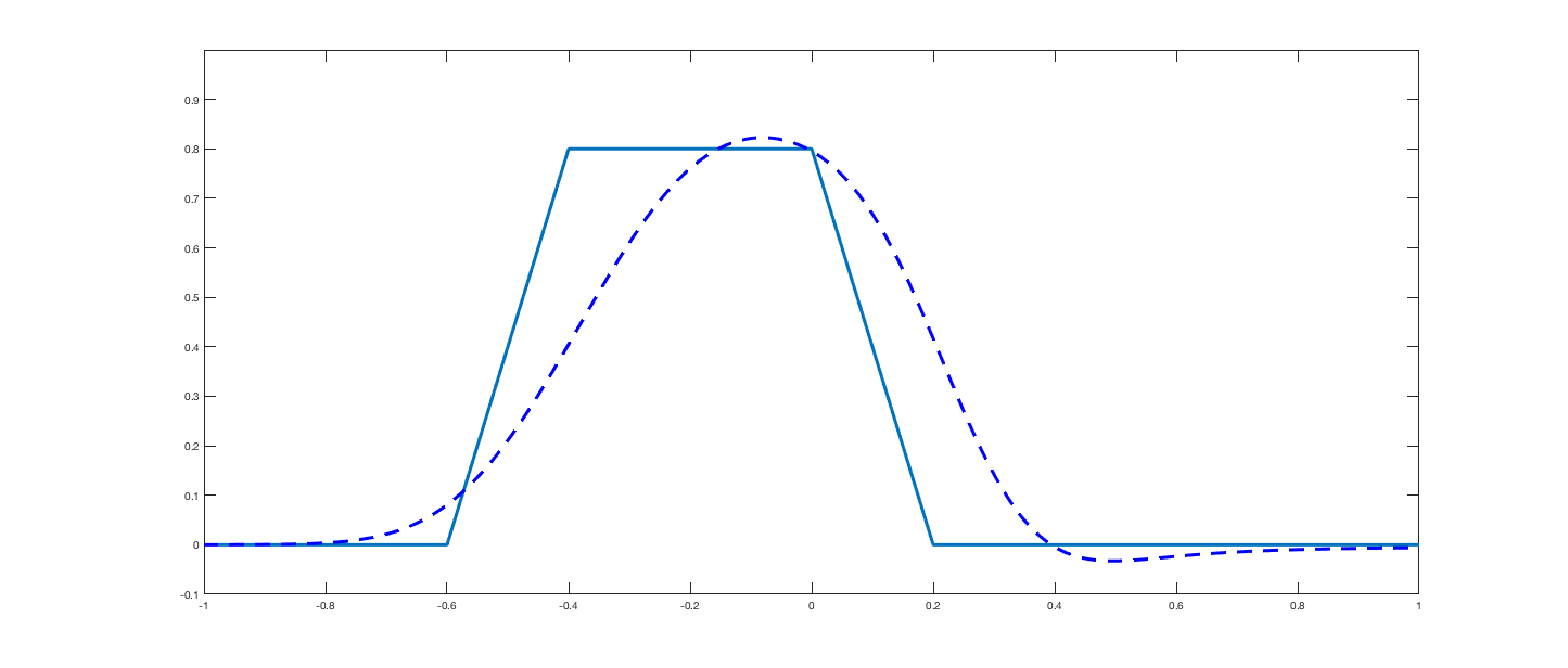
Figure 1. Example 1: $r=2$, $T=0.1$ and $N=640$

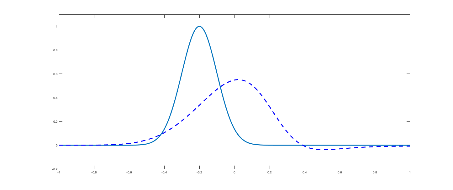
Figure 2. Example 2: $r=3$, $T=0.2$ and $N=640$

The numerical rate of convergence for the solutions in Figures 1 and 2 are presented in Tables 1 and 2.

$N$	error	relative error	order
20	4.0759e-04	4.3296e-04	1.9532
40	1.0526e-04	1.1181e-04	1.9173
80	2.7867e-05	2.9601e-05	1.7207
160	8.4546e-06	8.9808e-06	-

Table 1. Example 1: Error, relative error and numerical rate of convergence for one order polynomial approximations ($r=2$). $N$ denotes the number of elements.

$N$	error	relative error	order
20	1.0381e-04	3.1458e-04	2.3097
40	2.0939e-05	6.3452e-05	2.0792
80	4.9551e-06	1.5015e-05	1.8057
160	1.4174e-06	4.2952e-06	-

Table 2. Example 2: Error, relative error and numerical rate of convergence for second order polynomial approximations ($r=3$). $N$ denotes the number of elements.

We have measured the $L^{2}$-error

$$E_{h}=||u_{h}(T,\cdot)-\hat{u}_{e}(T,\cdot)||^{2},$$

where $\hat{u}_{e}$ is the numerical solution which has been computed using a very fine grid $h=2/640$. We also have measured the relative error

$$R_{h}=\left(\frac{1}{||\hat{u}_{e}(T,\cdot)||^{2}}\right)E_{h},$$

and the approximation rate of convergence

$$\alpha_{h}=\left(\frac{1}{\log 2}\right)\left(\log E_{h}-\log E_{h/2}\right).$$

We observe that the order of convergence is reached, confirming the theoretical results. Indeed, the experimental rates of convergence are greather than one for the first numerical example ($r=2$) and for the second example ($r=3$), the numerical rates of convergence are near to 2.

References

- [1] G. D. Akrivis, Finite element discretization of the Kuramoto-Sivashinsky equation, Numerical analysis and mathematical modelling, 29 (1994), pp. 155 – 163.
- [2] N. Alibaud, P. Azerad, and D. Isèbe, A non-monotone nonlocal conservation law for dune morphodynamics, Differential Integral Equations, 23 (2010), pp. 155–188.
- [3] A. Bouharguane and R. Carles, Splitting methods for the nonlocal fowler equation, Mathematics of Computation, 83 (2014).
- [4] F. E. Browder, Existence and uniqueness theorems for solutions of nonlinear boundary value problems, Proc. Sympos. Appl. Math., Vol. XVII, (1965), pp. 24–49.
- [5] J. Droniou, A numerical method for fractal conservation laws, Mathematics of Computation, 79 (2010), pp. 95–124.
- [6] G. J. Fix and J. P. Roof, Least squares finite-element solution of a fractional order two-point boundary value problem, Computers Mathematics with Applications, 48 (2004), pp. 1017–1033.
- [7] A. C. Fowler, Dunes and drumlins, in Geomorphological fluid mechanics, A. Provenzale and N. Balmforth, eds., vol. 211, Springer-Verlag, Berlin, 2001, pp. 430–454.
- [8] Q. Guan and M. Gunzburger, -schemes for finite element discretization of the space-time fractional diffusion equations, Journal of Computational and Applied Mathematics, 288 (2015), pp. 264 – 273.
- [9] F. Liu, V. Anh, and I. Turner, Numerical solution of the space fractional fokker–planck equation, Journal of Computational and Applied Mathematics, 166 (2004), pp. 209 – 219. Proceedings of the International Conference on Boundary and Interior Layers - Computational and Asymptotic Methods.
- [10] M. M. Meerschaert and C. Tadjeran, Finite difference approximations for fractional advection-dispersion flow equations, Journal of Computational and Applied Mathematics, 172 (2004), pp. 65 – 77.
- [11] J. P. Roop, Computational aspects of fem approximation of fractional advection dispersion equations on bounded domains in , Journal of Computational and Applied Mathematics, 193 (2006), pp. 243 – 268.
- [12] V. Thomée, Galerkin finite element methods for parabolic problems, Springer Series in Computational Mathematics, (2006).
- [13] Q. Xu and J. S. Hesthaven, Discontinuous Galerkin method for fractional convection-diffusion equations, SIAM Journal on Numerical Analysis, 52 (2014), pp. 405 – 423.
- [14] Y. Zheng, C. Li, and Z. Zhao, A note on the finite element method for the space-fractional advection diffusion equation, Computers Mathematics with Applications, 59 (2010), pp. 1718–1726.