Characterizing the Ly$\alpha$ forest flux probability distribution function using Legendre polynomials

Abstract

The Lyman-$\alpha$ forest is a highly non-linear field with considerable information available in the data beyond the power spectrum. The flux probability distribution function (PDF) has been used as a successful probe of small-scale physics. In this paper we argue that measuring coefficients of the Legendre polynomial expansion of the PDF offers several advantages over measuring the binned values as is commonly done. In particular, the $n$-th Legendre coefficient can be expressed as a linear combination of the first $n$ moments, allowing these coefficients to be measured in the presence of noise and allowing a clear route for marginalisation over mean flux. Moreover, in the presence of noise, our numerical work shows that a finite number of coefficients are well measured with a very sharp transition into noise dominance. This compresses the available information into a small number of well-measured quantities. We find that the amount of recoverable information is a very non-linear function of spectral noise that strongly favors fewer quasars measured at better signal to noise.

1 Introduction

The Ly$\alpha$ forest, seen as absorption lines of neutral hydrogen along the line-of-sight in quasar spectra, has become a powerful tracer of the underlying matter distribution at high redshift. Its multiple statistics [1], ranging from the evolution of the mean flux with redshift, the transmitted flux probability distribution function (PDF), to the two-point statistics of the power spectrum and correlation function, have been successfully used to probe cosmological parameters (as seen in [2, 3, 4, 5, 6, 7, 7, 8, 9, 10, 11] for example).

The flux PDF in particular has been studied since [12] as a way to understand the amplitude of matter fluctuations and the thermal history of the intergalactic medium (IGM). There has been much renewed interest in the flux PDF, since [13] and [14] have found a possible inverted temperature-density relation at $2<z<3$ with high resolution, high signal-to-noise (S/N) spectra. This would be in contrast to the theoretical predictions of a positive relation of $T\sim\rho^{\gamma}$, with $\gamma\sim 1.6$. Most recently, [15] revisited this question with stacked low resolution Sloan Digital Sky Survey (SDSS) spectra and found no such inversion. The flux PDF is therefore an ongoing probe of interest.

However, in addition to being sensitive to the cosmological evolution above, it is also dependent on the pixel noise level, the resolution of the spectra, and the systematic uncertainties in fitting the continuum level [15]. Therefore, the proper treatment of these errors is crucial. [1] first demonstrated the importance of using covariance matrices instead of the pure diagonal error bars in flux PDF measurements. The problem arises with the inversion of this flux PDF covariance matrix, as it is exactly singular [16] due to the normalization integral constraint, making it unnecessarily difficult to calculate noise and correctly fit predicted models [15].

Here we present an alternative way of encoding the same information, which is arguably systematically cleaner and conceptually nicer.

2 Shifted Legendre polynomial expansion

The flux field is a three-dimensional field defined through the 3D space

$$F(\mathbf{x})=e^{-\tau(\mathbf{x})}=\bar{F}\left(1+\delta_{F}(\mathbf{x})\right),$$ (2.1)

where $\tau(\mathbf{x})$ is the optical depth due to the Ly$\alpha$ forest, $\bar{F}$ is the mean flux and $\delta_{F}$ are variations around this mean flux. The statistical properties of this field are completely described by the full set of $n$-correlation functions $\left<F(\mathbf{x})\cdots F(\mathbf{x}^{\prime})\right>$. Usually we measure the 2-point function in real or Fourier space, but considerable information is present in the field beyond these two. [17] demonstrates that the 1D bispectrum contains at least the same amount of information as the 1D power spectrum. Alternatively, and perhaps somewhat easier routes are via PDFs. After optionally smoothing the field on a certain scale (e.g., due to the instrumental resolution of a spectrograph), the flux PDF $P(F)dF$ is defined as the probability of the flux being between $F$ and $F+dF$ for a randomly chosen point. This function is uniquely determinable from all possible cumulants (which are in turn given by moments) of the input field and of course also depends on smoothing.

The zeroth moment of the field is unity and the first moment gives the mean flux:

$$\int_{0}^{1}P(F)dF = 1,$$ (2.2)

$$\int_{0}^{1}FP(F)dF = \bar{F}.$$ (2.3)

Traditionally, the flux PDF has been measured in $i=1\ldots N$ bins of flux, defined by

$$B_{i}=\int_{(i-1)/N}^{i/N}P(F)dF$$ (2.4)

This gives the constraint $\sum B_{i}=1$. While one can write a Bayesian estimator for $B_{i}$, it is clear that at least the covariance matrix of the measured $B_{i}$ will be non-positive definite, since the linear combination of $\sum B_{i}$ modes has zero variance and hence the corresponding eigenvalue is zero, making the covariance matrix strictly non-positive definite. There are robust ways of dealing with this. For example, one can diagonalize the matrix and use the $N-1$ non-zero eigenvectors to determine $\chi^{2}$. Alternatively, one can simply drop one of the bins (since its value is completely determined by the sum constraint). However, while matrix inversion is a nuissance, there are two more significant problems. First, in the presence of noise, a simple binning of flux will not give an unbiased estimate of $B_{i}$. Second, unless one deals with very high signal-to-noise ratio (SNR) data measured at very high resolution, we can only measure values of $\delta_{F}$ rather than $F$ and hence some marginalisation over $\bar{F}$ is required.

Here we propose an alternative, namely to expand $P(F)$ in terms of shifted Legendre polynomials $L_{\ell}(x)=\tilde{L}_{\ell}(2x-1)$, where $\tilde{L}_{\ell}$ are the standard, unshifted polynomials defined between $-1$ and $+1$ and $L_{\ell}(F)$ are the shifted version defined between $0$ and $1$. Given that this is a complete orthonormal basis, we have:

$$P(F) = \sum_{\ell=0}^{\infty}a_{\ell}L_{\ell}(F),$$ (2.5)

$$a_{\ell} = (2\ell+1)\int_{0}^{1}P(F)L_{\ell}(F)dF$$ (2.6)

The first few polynomials are given by

$$L_{0}(F) = 1$$ (2.7)

$$L_{1}(F) = 2F-1$$ (2.8)

$$L_{2}(F) = 6F^{2}-6F+1$$ (2.9)

$$L_{3}(F) = 20F^{3}-30F^{2}+12F-1$$ (2.10)

$$L_{4}(F) = 70F^{4}-140F^{3}+90F^{2}-20F+1$$ (2.11)

$$\cdots$$ (2.12)

Using standard properties of Legendre polynomials, one finds that moments of the flux field are given by

$$M_{n}=\left<F^{n}\right>=\sum_{l=0}^{n}\frac{a_{\ell}n!^{2}}{(n-l)!(n+l+1)!}.$$ (2.13)

This result is crucial since we have made an explicit link between the moments of the distribution and the PDF. More importantly, we have also shown that the first $n$ coefficients $a_{\ell}$ are completely determined by the first $n$ moments $M_{n}$.

These can be converted to the more observationally relevant quantity: the moments of $\delta_{F}$, given by $m_{n}=\left<\delta_{F}^{n}\right>$, with $m_{0}=1$, $m_{1}=0$. Here we have

$$M_{n}=\bar{F}^{n}\sum_{k=0}^{n}{{n}\choose{k}}m_{n-k}.$$ (2.14)

We can therefore express the coefficients of our polynomial expansion $a_{\ell}$ combinatorially from observed moments $M_{n}$ or $m_{n}$ as

$$a_{0} = 1$$ (2.15)

$$a_{1} = 6M_{1}-3$$ (2.16)

$$a_{2} = 30M_{2}-30M_{1}+5=30\bar{F}^{2}m_{2}+30\bar{F}^{2}-30\bar{F}+5$$ (2.17)

$$a_{3} = 140M_{3}-210M_{2}+84M_{1}-7$$

$$= 140\,{\bar{F}}^{3}{m_{{3}}}+420\,{\bar{F}}^{3}{m_{{2}}}-210\,{\bar{F}}^{2}{m_{{2}}}+140\,{\bar{F}}^{3}-210\,{\bar{F}}^{2}+84\,\bar{F}-7$$

$$a_{4} = 630M_{4}-1260M_{3}+810M_{2}-180M_{1}+9$$

$$= 630\,{\bar{F}}^{4}{m_{{4}}}+2520\,{\bar{F}}^{4}{m_{{3}}}-1260\,{\bar{F}}^{3}{m_{{3}}}+3780{\bar{F}}^{4}{m_{2}}-3780\,{\bar{F}}^{3}{m_{{2}}}$$

$$+810\,{\bar{F}}^{2}{m_{{2}}}+630{\bar{F}}^{4}-1260\,{\bar{F}}^{3}+810\,{\bar{F}}^{2}-180\,\bar{F}+9$$

$$\cdots$$ , (2.20)

where $M_{1}=\bar{F}$. We now see that there are three equivalent complete descriptions of the probability distribution function. The first one is in terms of binned PDF parameters $B_{i}$, the second one is in terms of either moments $M_{n}$ or central normalized moments $m_{n}$, and the third one is in terms of coefficients of Legendre polynomials $a_{\ell}$, which are completely given by the moments and allow one to “reconstruct” the actual PDF. Although the above equations might seem unnecessarily complicated, we note that these are trivially generated algorithmically to an arbitrary order.

We also note that from the observational perspective, using moments or $a_{\ell}$ coefficients has a distinct advantage in that it is clear how the noise and $\bar{F}$ uncertainty enter the measurement. With respect to the noise, the measurement of the $i$-th coefficient requires one to measure the noise-subtracted $i$-th moment. For a purely Gaussian noise, this is trivial, but any non-Gaussianity will contaminate $i>2$ measurements, probably progressively so. Therefore, in the presence of noise, it is unlikely that one can measure, with very high precision more than a few first coefficients $a_{\ell}$. On the side of $\bar{F}$, its determination requires modeling of the unabsorbed continuum level, which is only possible for spectra of extremely high signal to noise and sufficient number of unabsorbed pixels [18]. In our case, any uncertainty in $\bar{F}$ can be propagated in a fully understood manner into the covariance matrix for the final measurement, since we know exactly how it enters the measurement of the polynomial coefficients.

Finally, this method makes the complementarity with power spectrum calculations easier to understand. The power-spectrum is quadratic in the flux field data and hence the $a_{2}$ coefficient (or equivalently the second moments), as a function of the smoothing scale, are completely determined by the measurement of the power spectrum and the mean flux. The measurement of $a_{3}$ as a function of smoothing scale is akin to a reduced bispectrum, etc.

3 Demonstration on simulations

To demonstrate this method numerically, we use the PDF generated from full hydrodynamic Gadget-3 simulations [19], evolved to redshift 2, with a WMAP7 cosmology, where $\Omega_{\mathrm{m}}=0.275$, $\Omega_{\Lambda}=0.725$, $\Omega_{\mathrm{b}}=0.046$, $h_{0}=0.702$, $\sigma_{8}=0.816$, and $\mathrm{n}_{\mathrm{s}}=0.96$. The box size evolved is 80 Mpc/h, with $N=2\times 512^{3}$ for the number of gas and dark matter particles, and a Haardt and Madau UV background [20]. The simple QUICKLYA option is used for star formation with no feedback. We generate a flux PDF from simulated mock Lyman-$\alpha$ forest spectra that have been convolved with the line profile, with the lines of sight on a $512\times 512$ matrix on $1024$ pixel-long skewers. In this demonstration we will consider a rough equivalent of the BOSS experiment [21] and thus we apply a Gaussian smoothing on the scale of $1h/$Mpc in the radial direction to simulate the equivalent spectroscopic resolution. This noiseless PDF is pictured in Figure 1 as the black solid line. Since resolution requirements increase with redshift, we use the redshift 2 output for our method demonstration, however we note that our simulation might not fully resolve the extreme fluxes at both ends of the PDF, as noted in convergence studies of [22] and [23]. For this example exercise, to overcome the shortcoming of a small box size, we use this PDF as a representative PDF and generate new skewers with pixels drawn independently from this PDF. In order to calculate the covariance matrix for the flux PDF and the subsequent method covariance matrices, we draw points representing 160,000 quasars of 200 pixels each to represent a BOSS-scale experiment [21], applying the bootstrap method with 1000 for the number of resamples.

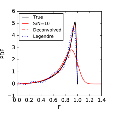
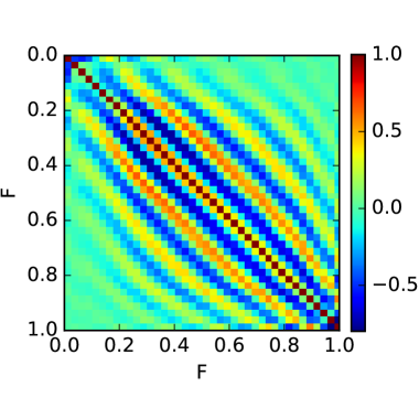
Figure 1: True PDF, smoothed with 1 Mpc/h in line-of-sight direction (black solid line), PDF with S/N=10 (red solid line), deconvolved with n=40 (red dashed line) along with the corresponding covariance matrix (right side), and legendre reconstruction with 40 coefficients (dotted blue line).

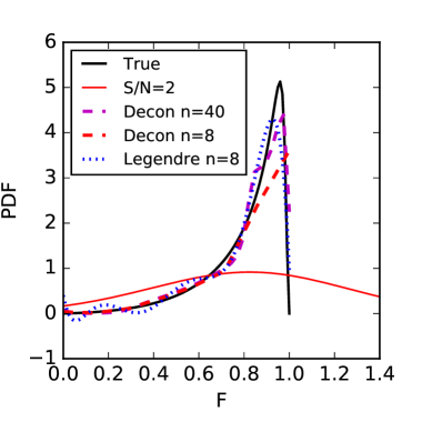
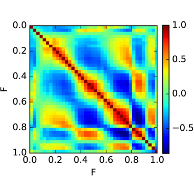
Figure 2: True PDF, smoothed with 1 Mpc/h in line-of-sight direction (black solid line), PDF with S/N=2 (red solid line), deconvolved with n=40 (magenta dashed line) along with the corresponding covariance matrix (right side), deconvolved with n=8 (red dashed line), and legendre reconstruction with 8 coefficients (dotted blue line).

3.1 PDF maximum likelihood noise deconvolution

Next we add varying amount of noise to the data.For the first example, the thin red line in Figure 1 shows the smoothed binned PDF for a SNR of 10, where we did not attempt to reconstruct the input PDF. The effect of noise is to broaden the values of flux beyond the physically allowed range $0-1$ and demonstrates that a full forward-modeling is required to reconstruct the input flux PDF.

We first demonstrate a reconstruction of the original PDF using a maximum likelihood noise deconvolution method for this toy model. We’d like to recover the reconstructed PDF divided into $n$ bins, where the response of the $n$-th bin to noise spreads the flux values into the observed $i$ bins. At fixed noise, the analysis simplifies considerably. The observed $i$-th bin of the flux PDF can therefore be modeled by the convolution of the reconstructed bins $B^{r}$ with the response $p_{i}$ of the $n$-th bin to noise:

$$B_{i}^{o}=B^{r}*p_{i}=\sum\limits_{n}B^{r}_{n}p_{i-n}.$$ (3.1)

Using the cumulative distribution function for a Gaussian noise distribution:

$$F_{n}(i)=\frac{1}{2}\left[1+\mathrm{erf}\left(\frac{i-n}{\sqrt{2}\sigma_{\mathrm{noise}}}\right)\right],$$ (3.2)

we can model the response of the $n$-th bin to noise as

$$p_{i-n}=F_{n}(i+1)-F_{n}(i)=F_{i}(n)-F_{i}(n-1),$$ (3.3)

where we have used $\mathrm{erf}(-x)=-\mathrm{erf}(x)$. For each bootstrap iteration we therefore can maximize the likelihood by minimizing

$$\chi^{2}=\sum\limits_{i}\frac{\left(B_{i}^{o}-B^{r}*p_{i}\right)^{2}}{B^{r}*p_{i}}$$ (3.4)

to arrive at the reconstructed PDF bins $B^{r}$. The mean of the reconstructed PDFs is pictured as the red dashed line in Figure 1 for $n$=40 bins, with the associated covariance matrix between the bootstrap iterations on the right hand side of the same figure. As one can see, the fit to the original PDF is very good, however the covariance matrix for noise estimation has complex structure. In addition, as we go to lower SNR the fit worsens, as is seen in Figure 2, and the covariance matrix retains its complex structure. In addition, as we decrease the number of reconstructed points, the fit becomes drastically worse, even though the reconstruction is quite good using the same lower number of Legendre coefficients, as described in the next section. Figure 2 shows the reconstruction for $n=8$ points, and the same for 8 measured Legendre coefficients. The $n=40$ bin points shows a similar fit to the PDF despite five fold increase in the number of points. In fact the number of well measured modes is very few as we demonstrate next. We take the 40 bin covariance matrices and decompose them into eigenvectors and eigenvalues. We then project the true model into this eigenspace and calculate the signal-to-noise for each eigenvector, i.e.

$${\rm(SNR)}_{i}^{2}=\frac{(\mathbf{v}_{i}\cdot\mathbf{t})^{2}}{\lambda_{i}},$$ (3.5)

where $\lambda_{i}$ and $v_{i}$ are the $i$-th eigenvalue and eigenvector, respectively, and $t$ is the vector containing the true model (i.e. 40 bins representing the PDF). We then order in decreasing SNR and calculate the cumulative SNR by summing individual contributions in quadrature. The results are plotted in Figure 3. We see the expected behavior: out of 40 points, the total SNR in PDF determination is concentrated in a few linear combinations and the number of such combinations decreases with spectral SNR. As we will see later the Legendre polynomial decomposition is only slightly worse and compresses information into a few well-measured modes.

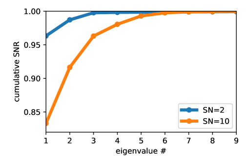
Figure 3: The normalized cumulatative signal to noise derived from covariance matrices from Figures 1 and 2 as described in the text. We infer that all information is compressed in $\sim$4 modes for spectral SN$\sim 2$ and $\sim 8$ modes for spectral SN$\sim 5$.

We can conclude that the deconvolution method works well for high SNR but does not work as well for a given number of points as we decrease the SNR. In addition, the covariance matrix of the deconvolved PDF has complex structure.

3.2 Moments and Legendre coefficients

We then calculate moments $M_{i}$ by measuring raw moments in the data and then subtracting the noise contribution:

$$\tilde{M_{i}}=\frac{1}{N_{\rm points}}\sum_{k}F_{k}^{i}-N_{i},$$ (3.6)

where $N_{2}=\sigma^{2}$, $N_{3}=3\bar{F}\sigma^{2}$, $N_{4}=6\tilde{M_{2}}\sigma^{2}+3\sigma^{4}$, etc. with $\sigma^{2}$ being the variance of the error. This procedure can be trivially generalized to real data with varying noise. This allows us to reconstruct values of $a_{\ell}$ and estimate the uncertainty. Since the coefficients $a_{\ell}$ are linear in $M_{i}$, our estimates for $a_{\ell}$ are unbiased. The results of this exercise are plotted in Figure 4. We see that the addition of noise degrades measurements as expected. However, the effect is considerably more dramatic for the $a_{\ell}$ parameterization than it is for moments. For moments we note a slow increase in the uncertainties with errors on $M_{10}$ increasing markedly at low $S/N$ but barely perceptible in others. On the other hand for $a_{\ell}$ coefficients, we note a noise-level dependent “wall” in $\ell$: for SNR around $1$, there is virtually no information at $\ell>6$ and for SNR around $2$, the same is true for $\ell>8$. In other words, the transformation is very successful at compressing the information content into a few well-measured numbers.

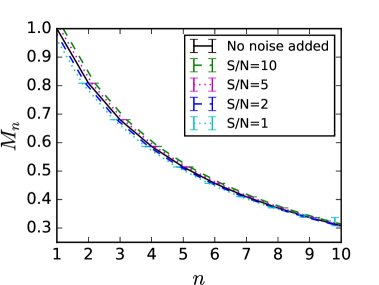
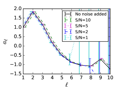
Figure 4: Values of $M_{n}$ in left panel and the reconstructed Legendre polynomial coefficients $a_{\ell}$ in the right panel after adding Gaussian noise for a signal-to-noise ratio of 1 (cyan dotted line), 2 (blue dashed line), 5 (magenta dotted line), 10 (green dashed line). The no noise added line is represented as a black continuous line. The lines are offset horizontally to better visualize the change in error bars.

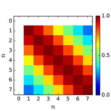
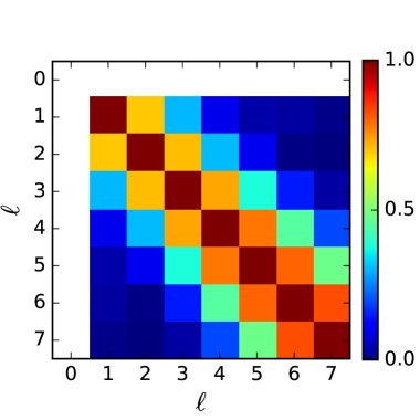
Figure 5: Values of the reconstructed $M_{n}$ covariance matrix in the left panel, and the reconstructed Legendre polynomial coefficients $a_{l}$ covariance matrix in the right panel, both for a signal-to-noise ratio of 2 (represented as blue dashed line in Figure 4).

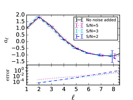
Figure 6: Reconstructed $a_{l}$ coefficients for 160,000 quasars with a signal-to-noise of 2 (blue dashed line), 5,000 quasars with a signal-to-noise of 3 (cyan dotted line), and 25 quasars with a signal-to-noise of 5 (magenta dotted line). The bottom panel shows errors. This plot illustrates that higher spectral SNR measurements allow determination of a larger number of Legendre coefficients at very modest number of quasars.

In Figure 5 we show the covariance matrix for moments and Legendre polynomial coefficients for SNR $\sim 2$. We see that well-determined moments are heavily correlated, but that the poorly determined ones are virtually uncorrelated. The correlation in the low $\ell$ modes most likely comes from sample variance which dominates their determination.

Figure 1 shows the reconstructed PDF against the input PDF for the most likely solution. This is a sanity check. We see that SNR $\sim 10$ “reconstructs” the true PDF very well.

Since there is a finite number of $a_{\ell}$ values that can be measured well for a given SNR, it is worth exploring the number of quasars at higher SNR that would give the same number of well-measured Legendre coefficients. In Figure 6 we plot the values of $a_{\ell}$ for SNR=2 for the 160,000 quasars as explored earlier and we also plot results for 5000 SNR=3 quasars and just 5 SNR=5 quasars. We find that the large number of low SNR quasars is only helpful at the first few coefficients and even there the required numbers is disproportionally large.

4 Conclusions

The properties of a random field are completely determined by the full set of $n$-point correlators. Any derived quantity such as PDF can in principle be derived from them.

In this paper we have made the link explicit for the Lyman-$\alpha$ forest flux, or any other field, for which the values of the field are limited to be in the finite range. We have shown that the first $n$ moments of the field uniquely determined the first $n$ $a_{\ell}$ coefficients in the Legendre polynomial expansion of the PDF and vice-versa.

Using a toy-example, we argue that instead of measuring PDF, one should measure the $a_{\ell}$ coefficients. There are four main reasons for this:

• In our toy example these coeffients are very good at sorting the information content available in the PDF into a few well determined numbers and an infinite number of very poorly determined numbers. The precise number of well-determined coefficients is given by the SNR of the available data.

• Our procedure provides a very clear path to measuring these quantities: $a_{\ell}$ coefficients can be determined from the moments of the field for which unbiased estimators in the presence of noise are trivially computed.

• Mean flux $\bar{F}$ is difficult to measure in real data and must be marginalised out assuming a plausible prior. Since $\bar{F}$ is just the first moment of the field, this marginalization is considerably easier than in the case of fitting a binned flux distribution function.

• If $a_{\ell}$ coefficients are measured at a number of smoothing scales, a considerable statistical information is contained in a 2D field $a_{\ell}(k_{s})$ with $k_{s}$ being the smoothing wavenumber. In particular, assuming $\bar{F}$ to be known, the $a_{2}(k_{s})$ contains the same information as the 1D power spectrum.

Before this method can be put in practice, more work needs to be done. On the observational side, the effects of metal contamination and damped Lyman-$\alpha$ systems need to be understood. On the theoretical side, more work needs to be done to establish the relation between these coefficients and physical properties of the intergalactic medium, such as its mean flux or temperature-density relation. We leave this for future work.

Another important result of this paper is how non-linear the degradation in ability to characterize the PDF is with spectral SNR. We find that, neglecting sample variance, using 25 quasars of SNR=5 yields comparable results to 160,000 quasars of SNR=2. Although the latter measures the first few Legendre modes somewhat better, the former measures a larger number of the modes. In retrospect, one would expect this, because the PDF depends on all moments of the field and the measurements of higher modes are of course more sensitive to noise. But it is nevertheless quite striking just how large this sensitivity is.

References

- [1] P. McDonald, J. Miralda-Escudé, M. Rauch, W. L. W. Sargent, T. A. Barlow, R. Cen, and J. P. Ostriker, The Observed Probability Distribution Function, Power Spectrum, and Correlation Function of the Transmitted Flux in the Ly Forest, ApJ 543 (Nov., 2000) 1–23.
- [2] M. Viel, G. D. Becker, J. S. Bolton, and M. G. Haehnelt, Warm dark matter as a solution to the small scale crisis: New constraints from high redshift Lyman- forest data, Phys. Rev. D 88 (Aug., 2013) 043502, [arXiv:1306.2314].
- [3] U. Seljak, A. Makarov, P. McDonald, and H. Trac, Can Sterile Neutrinos Be the Dark Matter?, Physical Review Letters 97 (Nov., 2006) 191303–+.
- [4] N. Afshordi, P. McDonald, and D. N. Spergel, Primordial Black Holes as Dark Matter: The Power Spectrum and Evaporation of Early Structures, ApJ 594 (Sept., 2003) L71–L74.
- [5] N. Palanque-Delabrouille, C. Yèche, J. Lesgourgues, G. Rossi, A. Borde, M. Viel, E. Aubourg, D. Kirkby, J.-M. LeGoff, J. Rich, N. Roe, N. P. Ross, D. P. Schneider, and D. Weinberg, Constraint on neutrino masses from SDSS-III/BOSS Ly forest and other cosmological probes, JCAP 2 (Feb., 2015) 45, [arXiv:1410.7244].
- [6] J. Lesgourgues, G. Marques-Tavares, and M. Schmaltz, Evidence for dark matter interactions in cosmological precision data?, ArXiv e-prints (July, 2015) [arXiv:1507.04351].
- [7] U. Seljak, A. Slosar, and P. McDonald, Cosmological parameters from combining the Lyman- forest with CMB, galaxy clustering and SN constraints, Journal of Cosmology and Astro-Particle Physics 10 (Oct., 2006) 14–+.
- [8] C. Dvorkin, K. Blum, and M. Kamionkowski, Constraining dark matter-baryon scattering with linear cosmology, Phys. Rev. D 89 (Jan., 2014) 023519, [arXiv:1311.2937].
- [9] N. G. Busca, T. Delubac, J. Rich, S. Bailey, A. Font-Ribera, D. Kirkby, J.-M. Le Goff, M. M. Pieri, A. Slosar, É. Aubourg, J. E. Bautista, D. Bizyaev, M. Blomqvist, A. S. Bolton, J. Bovy, H. Brewington, A. Borde, J. Brinkmann, B. Carithers, R. A. C. Croft, K. S. Dawson, G. Ebelke, D. J. Eisenstein, J.-C. Hamilton, S. Ho, D. W. Hogg, K. Honscheid, K.-G. Lee, B. Lundgren, E. Malanushenko, V. Malanushenko, D. Margala, C. Maraston, K. Mehta, J. Miralda-Escudé, A. D. Myers, R. C. Nichol, P. Noterdaeme, M. D. Olmstead, D. Oravetz, N. Palanque-Delabrouille, K. Pan, I. Pâris, W. J. Percival, P. Petitjean, N. A. Roe, E. Rollinde, N. P. Ross, G. Rossi, D. J. Schlegel, D. P. Schneider, A. Shelden, E. S. Sheldon, A. Simmons, S. Snedden, J. L. Tinker, M. Viel, B. A. Weaver, D. H. Weinberg, M. White, C. Yèche, and D. G. York, Baryon acoustic oscillations in the Ly forest of BOSS quasars, A&A 552 (Apr., 2013) A96, [arXiv:1211.2616].
- [10] A. Slosar, V. Iršič, D. Kirkby, S. Bailey, N. G. Busca, T. Delubac, J. Rich, É. Aubourg, J. E. Bautista, V. Bhardwaj, M. Blomqvist, A. S. Bolton, J. Bovy, J. Brownstein, B. Carithers, R. A. C. Croft, K. S. Dawson, A. Font-Ribera, J.-M. Le Goff, S. Ho, K. Honscheid, K.-G. Lee, D. Margala, P. McDonald, B. Medolin, J. Miralda-Escudé, A. D. Myers, R. C. Nichol, P. Noterdaeme, N. Palanque-Delabrouille, I. Pâris, P. Petitjean, M. M. Pieri, Y. Piškur, N. A. Roe, N. P. Ross, G. Rossi, D. J. Schlegel, D. P. Schneider, N. Suzuki, E. S. Sheldon, U. Seljak, M. Viel, D. H. Weinberg, and C. Yèche, Measurement of baryon acoustic oscillations in the Lyman- forest fluctuations in BOSS data release 9, JCAP 4 (Apr., 2013) 26, [arXiv:1301.3459].
- [11] T. Delubac, J. E. Bautista, N. G. Busca, J. Rich, D. Kirkby, S. Bailey, A. Font-Ribera, A. Slosar, K.-G. Lee, M. M. Pieri, J.-C. Hamilton, É. Aubourg, M. Blomqvist, J. Bovy, J. Brinkmann, W. Carithers, K. S. Dawson, D. J. Eisenstein, S. G. A. Gontcho, J.-P. Kneib, J.-M. Le Goff, D. Margala, J. Miralda-Escudé, A. D. Myers, R. C. Nichol, P. Noterdaeme, R. O’Connell, M. D. Olmstead, N. Palanque-Delabrouille, I. Pâris, P. Petitjean, N. P. Ross, G. Rossi, D. J. Schlegel, D. P. Schneider, D. H. Weinberg, C. Yèche, and D. G. York, Baryon acoustic oscillations in the Ly forest of BOSS DR11 quasars, A&A 574 (Feb., 2015) A59, [arXiv:1404.1801].
- [12] E. B. Jenkins and J. P. Ostriker, Lyman-alpha depression of the continuum from high-redshift quasars - A new technique applied in search of the Gunn-Peterson effect, ApJ 376 (July, 1991) 33–42.
- [13] J. S. Bolton, M. Viel, T.-S. Kim, M. G. Haehnelt, and R. F. Carswell, Possible evidence for an inverted temperature-density relation in the intergalactic medium from the flux distribution of the Ly forest, MNRAS 386 (May, 2008) 1131–1144, [arXiv:0711.2064].
- [14] M. Viel, J. S. Bolton, and M. G. Haehnelt, Cosmological and astrophysical constraints from the Lyman forest flux probability distribution function, MNRAS 399 (Oct., 2009) L39–L43, [arXiv:0907.2927].
- [15] K.-G. Lee, J. F. Hennawi, D. N. Spergel, D. H. Weinberg, D. W. Hogg, M. Viel, J. S. Bolton, S. Bailey, M. M. Pieri, W. Carithers, D. J. Schlegel, B. Lundgren, N. Palanque-Delabrouille, N. Suzuki, D. P. Schneider, and C. Yèche, IGM Constraints from the SDSS-III/BOSS DR9 Ly Forest Transmission Probability Distribution Function, ApJ 799 (Feb., 2015) 196, [arXiv:1405.1072].
- [16] A. Lidz, K. Heitmann, L. Hui, S. Habib, M. Rauch, and W. L. W. Sargent, Tightening Constraints from the Ly Forest with the Flux Probability Distribution Function, ApJ 638 (Feb., 2006) 27–44, [astro-ph/0505138].
- [17] R. Mandelbaum, P. McDonald, U. Seljak, and R. Cen, Precision cosmology from the Lyman- forest: power spectrum and bispectrum, MNRAS 344 (Sept., 2003) 776–788.
- [18] U. Seljak, P. McDonald, and A. Makarov, Cosmological constraints from the cosmic microwave background and Lyman- forest revisited, MNRAS 342 (July, 2003) L79–L84.
- [19] V. Springel, The cosmological simulation code GADGET-2, MNRAS 364 (Dec., 2005) 1105–1134, [astro-ph/0505010].
- [20] F. Haardt and P. Madau, Radiative Transfer in a Clumpy Universe. II. The Ultraviolet Extragalactic Background, ApJ 461 (Apr., 1996) 20–+.
- [21] K. S. Dawson, D. J. Schlegel, C. P. Ahn, S. F. Anderson, É. Aubourg, S. Bailey, R. H. Barkhouser, J. E. Bautista, A. Beifiori, A. A. Berlind, V. Bhardwaj, D. Bizyaev, C. H. Blake, M. R. Blanton, M. Blomqvist, A. S. Bolton, A. Borde, J. Bovy, W. N. Brandt, H. Brewington, J. Brinkmann, P. J. Brown, J. R. Brownstein, K. Bundy, N. G. Busca, W. Carithers, A. R. Carnero, M. A. Carr, Y. Chen, J. Comparat, N. Connolly, F. Cope, R. A. C. Croft, A. J. Cuesta, L. N. da Costa, J. R. A. Davenport, T. Delubac, R. de Putter, S. Dhital, A. Ealet, G. L. Ebelke, D. J. Eisenstein, S. Escoffier, X. Fan, N. Filiz Ak, H. Finley, A. Font-Ribera, R. Génova-Santos, J. E. Gunn, H. Guo, D. Haggard, P. B. Hall, J.-C. Hamilton, B. Harris, D. W. Harris, S. Ho, D. W. Hogg, D. Holder, K. Honscheid, J. Huehnerhoff, B. Jordan, W. P. Jordan, G. Kauffmann, E. A. Kazin, D. Kirkby, M. A. Klaene, J.-P. Kneib, J.-M. Le Goff, K.-G. Lee, D. C. Long, C. P. Loomis, B. Lundgren, R. H. Lupton, M. A. G. Maia, M. Makler, E. Malanushenko, V. Malanushenko, R. Mandelbaum, M. Manera, C. Maraston, D. Margala, K. L. Masters, C. K. McBride, P. McDonald, I. D. McGreer, R. G. McMahon, O. Mena, J. Miralda-Escudé, A. D. Montero-Dorta, F. Montesano, D. Muna, A. D. Myers, T. Naugle, R. C. Nichol, P. Noterdaeme, S. E. Nuza, M. D. Olmstead, A. Oravetz, D. J. Oravetz, R. Owen, N. Padmanabhan, N. Palanque-Delabrouille, K. Pan, J. K. Parejko, I. Pâris, W. J. Percival, I. Pérez-Fournon, I. Pérez-Ràfols, P. Petitjean, R. Pfaffenberger, J. Pforr, M. M. Pieri, F. Prada, A. M. Price-Whelan, M. J. Raddick, R. Rebolo, J. Rich, G. T. Richards, C. M. Rockosi, N. A. Roe, A. J. Ross, N. P. Ross, G. Rossi, J. A. Rubiño-Martin, L. Samushia, A. G. Sánchez, C. Sayres, S. J. Schmidt, D. P. Schneider, C. G. Scóccola, H.-J. Seo, A. Shelden, E. Sheldon, Y. Shen, Y. Shu, A. Slosar, S. A. Smee, S. A. Snedden, F. Stauffer, O. Steele, M. A. Strauss, A. Streblyanska, N. Suzuki, M. E. C. Swanson, T. Tal, M. Tanaka, D. Thomas, J. L. Tinker, R. Tojeiro, C. A. Tremonti, M. Vargas Magaña, L. Verde, M. Viel, D. A. Wake, M. Watson, B. A. Weaver, D. H. Weinberg, B. J. Weiner, A. A. West, M. White, W. M. Wood-Vasey, C. Yeche, I. Zehavi, G.-B. Zhao, and Z. Zheng, The Baryon Oscillation Spectroscopic Survey of SDSS-III, AJ 145 (Jan., 2013) 10, [arXiv:1208.0022].
- [22] Z. Lukić, C. W. Stark, P. Nugent, M. White, A. A. Meiksin, and A. Almgren, The Lyman forest in optically thin hydrodynamical simulations, MNRAS 446 (Feb., 2015) 3697–3724, [arXiv:1406.6361].
- [23] J. S. Bolton, E. Puchwein, D. Sijacki, M. G. Haehnelt, T.-S. Kim, A. Meiksin, J. A. Regan, and M. Viel, The Sherwood simulation suite: overview and data comparisons with the Lyman forest at redshifts 2 z 5, MNRAS 464 (Jan., 2017) 897–914, [arXiv:1605.03462].