Dynamic structure factor of a strongly correlated Fermi superfluid within a density functional theory approach

Abstract

We theoretically investigate the dynamic structure factor of a strongly interacting Fermi gas at the crossover from Bardeen-Cooper-Schrieffer superfluids to Bose-Einstein condensates, by developing an improved random phase approximation within the framework of a density functional theory - the so-called superfluid local density approximation. Compared with the previous random-phase-approximation studies based on the standard Bogoliubov-de Gennes equations, the use of the density functional theory greatly improves the accuracy of the equation of state at the crossover, and leads to a better description of both collective Bogoliubov-Anderson-Goldstone phonon mode and single-particle fermionic excitations at small transferred momentum. Near unitarity, where the $s$-wave scattering length diverges, we show that the single-particle excitations start to significantly contribute to the spectrum of dynamic structure factor once the frequency is above a threshold of the energy gap at $2\Delta$. The sharp rise in the spectrum at this threshold can be utilized to measure the pairing gap $\Delta$. Together with the sound velocity determined from the phonon branch, the dynamic structure factor provides us some key information of the crossover Fermi superfluid. Our predictions could be examined in experiments with ⁶Li or ⁴⁰K atoms using Bragg spectroscopy.

I Introduction

The realization of ultracold Fermi gases of ⁶Li and ⁴⁰K atoms near Feshbach resonances provides a new paradigm for studying strongly correlated many-body systems Bloch2008 . At low temperature, these systems display an intriguing crossover from Bardeen-Cooper-Schrieffer (BCS) superfluids to Bose-Einstein condensates (BEC)Leggett1980 ; Giorgini2008 . At a special point in between the two regimes, where the s-wave scattering length diverges, the gas exhibits universal properties, which might also exist in other strongly interacting Fermi superfluids Ho2004 ; Hu2007 , such as high-temperature superconductors or nuclear matter in neutron stars. This is called unitary Fermi gas and corresponds a novel type of superfluid with neither dominant bosonic nor fermionic character. This new superfluid has already been intensively investigated Giorgini2008 , leading to several milestone observations.

Theoretical challenges in describing the BCS-BEC crossover arise from its strongly correlated nature: there is no small interaction parameter to control the accuracy of theories Hu2010 . To date, significant progress has been made in developing better quantum Monte Carlo (QMC) simulations Astrakharchik2004 ; Bulgac2006 ; Burovski2008 ; Carlson2005 ; Carlson2008 ; Carlson2011 ; Forbes2011 ; Gandolfi2014 ; Carlson2014 and strong-coupling theories Ohashi2003 ; Liu2005 ; Chen2005 ; Hu2006 ; Haussmann2007 ; Diener2008 ; Mulkerin2016 , leading to the quantitative establishment of a number of properties in conjunction with the rapid experimental advances. These include the equation of state Hu2010 ; Luo2007 ; Nascimbene2010 ; Horikoshi2010 ; Navon2010 ; Ku2012 , frequency of collective oscillations Hu2004 ; Altmeyer2007 , pairing gap Carlson2005 ; Carlson2008 ; Schunck2007 ; Schirotzek2008 , and superfluid transition temperature Burovski2008 ; Ku2012 . However, some fundamental dynamical properties, such as the single-particle spectral function measured by radio-frequency (rf) spectroscopy Gaebler2010 ; Massignan2008 ; Chen2009 ; Hu2010PRL and the dynamic structure factor probed by Bragg spectroscopy Combescot2006 ; Veeravalli2008 ; Hu2012 ; Lingham2014 ; Vale2016 , are not well understood yet.

As an important fingerprint of quantum gases in some certain states, dynamic structure factor contains rich information of properties of a many-body system Pitaevskii2003 . By tuning the transferred momentum or energy from a low value to a high one, we can observe the low-lying collective phonon excitations, Cooper-pair (i.e., molecular) excitations and single-particle atomic excitations, respectively. In particular, at finite temperature the dynamic structure factor can help to judge whether the system is in the superfluid or normal state from the emergence of the phonon excitations. Also, it is reasonable to anticipate that the dynamic structure factor may play a role to solve the debate on the existence of pseudogap pairing or pre-pairing states Massignan2008 ; Chen2009 . Experimentally, the dynamic structure factor can be measured via two-photon Bragg scattering technique Veeravalli2008 , at both low and finite temperatures Lingham2014 . Theoretically, since no exact solution exists for strongly interacting Fermi gases and the numerically exact QMC approach is less efficient for simulating dynamical quantities, one has to resort to some approximated approaches, which are useful in certain limiting cases Hu2012 (see Table I). For example, at high temperature, as the fugacity is a small parameter, a quantum cluster expansion has been proven to be an efficient method Liu2009PRL ; Liu2013 , and has been used to calculate the dynamic structure factor Hu2010PRA ; Shen2013 . In the limits of both large momentum and high frequency, asymptotically exact Tan relations have been derived to describe the high-frequency tails Son2010 ; Hu2012PRA . On the other hand, in the limit of long wavelength or small momentum, the phenomenological two-fluid hydrodynamic theory may provide a useful description Hu2010NJP .

Theories	$q$ (applicable)	$T$ (applicable)
Virial expansion	arbitrary	$T>T_{F}$
Tan relation	$q\gg k_{F}$, $\omega\gg\varepsilon_{F}$	$T\gg T_{F}$
Two-fluid hydrodynamics	$q\ll k_{F}$,	$T<T_{c}$
Diagrammatic approach	arbitrary	arbitrary
BdG-RPA	$q\gg k_{F}$	$T\ll T_{c}$
SLDA-RPA (this work)	$q\lesssim k_{F}$	$T\ll T_{c}$

Table 1: A list of the existing theories for the dynamic structure of strongly interacting fermions, including the virial expansion Hu2010PRA ; Shen2013 , Tan relation Son2010 ; Hu2012PRA , two-fluid hydrodynamics Hu2010NJP , diagrammatic strong-coupling approach Palestini2012 ; He2016 , and BdG-RPA Combescot2006 ; Combescot2006EPL ; Zou2010 ; Guo2013 . The applicable conditions for the transferred momentum $q$ and temperature $T$, under which each theory is quantitatively useful, are indicated. Here $k_{F}=(3\pi^{2}n)^{1/3}$, $\varepsilon_{F}=k_{F}^{2}/(2m)=(3\pi^{2}n)^{2/3}/(2m),$ and $T_{F}$ are the Fermi momentum, energy, and temperature, respectively. $T_{c}$ is the superfluid transition temperature.

A general theoretical framework of the dynamic structure factor, valid at arbitrary temperature and momentum, can be developed by using the diagrammatic technique Guo2010 ; Palestini2012 or functional path integral approach He2016 , in parallel with the existing strong-coupling theories of interacting Fermi gases Hu2010 . The expressions for the density and spin responses of strongly interacting Fermi gases have been obtained He2016 . However, their numerical calculations turn out to be extremely difficult, except in the limit of zero transferred momentum Palestini2012 . A more commonly used approach is the random-phase approximation (RPA) on top of the mean-field Bogoliubov-de Gennes (BdG) theory Combescot2006 ; Combescot2006EPL ; Zou2010 ; Guo2013 . By comparing the BdG-RPA predictions with the experimental data for the dynamic structure factor of strongly interacting fermions and with the QMC results for the static structure factor Zou2010 , it has been surprisingly shown by two of the present authors that the BdG-RPA theory works quantitatively well at sufficiently large transferred momentum (i.e., $q\sim 5k_{F}$, where $k_{F}$ is the Fermi momentum). At small transferred momentum, i.e., $q\lesssim k_{F}$, apparently, the BdG-RPA only provides a qualitative description of the dynamic structure factor at the BCS-BEC crossover, since both the sound velocity (associated with the phonon excitations) and pairing gap (associated with the single-particle fermionic excitations) are strongly over-estimated within the BdG framework Giorgini2008 .

In this work, we aim to develop a quantitative theory for the dynamic structure factor of strongly interacting fermions at low transferred momentum and at low temperature, which is amenable for numerical calculations. For this purpose, we adopt a superfluid local density approximation (SLDA) approach Bulgac2002 ; Yu2003 ; Bulgac2007 , within the framework of density functional theory Hohenberg1964 ; Kohn1965 ; Kohn1999 , as recently suggested by Bulgac and his co-workers. The SLDA theory assumes an energy density functional (i.e., a function of the density function) to describe a unitary Fermi superfluid and uses the QMC results for the chemical potential and order parameter as two important inputs. It can be well regarded as a better quasi-particle description than the mean-field BdG theory. It has been shown that at low-energy the SLDA theory provides useful results for the equation of state Bulgac2007 and real-time dynamics Bulgac2011 ; Bulgac2013 of a strongly interacting Fermi superfluid.

Here we apply the random phase approximation on top of the SLDA theory. The use of SLDA in place of the standard BdG equations improves the predictions for the dynamic structure factor in the BCS-BEC crossover near unitarity. The static structure factor at small momentum transfer is in excellent agreement with the results of the latest QMC Gandolfi2014 ; Carlson2014 ; Combescot2006EPL . A more stringent test can be obtained in the near future by comparing our predictions with the experimental data Vale2016 , without any adjustable parameters.

Our paper is organized as follows. In the next section (Sec. II), we introduce the SLDA theory. In Sec. III, we review the main idea of RPA. The expression for the dynamic structure factor is derived in Sec. IV. In Sec. V and Sec. VI, we present our main results of dynamic structure factor in the unitary limit and the crossover regime, respectively. Finally, Sec. VII is devoted to conclusions and outlooks. For convenience, we set $\hbar=k_{B}=1$ in the following discussions.

II Superfluid local density approximation

The density functional theory (DFT) developed by Hohenberg and Kohn Hohenberg1964 , together with the local density approximation (LDA) by Kohn and Sham Kohn1965 , is a powerful tool to understand the properties of many-electron systems. The DFT was initially used for electrons in the normal, non-superconducting state. It is based on the assumptions that there is a unique mapping between the external potential and the total wave function of the system (or the normal density), and that the exact energy of the system can be written as a density functional. A limitation of the DFT is that the exact form of the density functional is often not known. Therefore, approximated phenomenological functionals are introduced, which should be optimized for a specific system. Typically, those functionals rely on the Kohn-Sham orbitals Kohn1999 and thus can not effectively deal with superfluidity. The generalization of the DFT to superfluid cold-atom systems - referred to as SLDA as we mentioned earlier - was recently introduced by Bulgac and Yu Bulgac2002 ; Yu2003 ; Bulgac2007 . This SLDA originates from a similar DFT previously used in the context of nuclear physics Yu2003 ; Bulgac2013 .

A nice feature of ultracold fermions is that, in the unitary limit the form of the energy density functional is restricted by dimensional arguments. Another advantage is the availability of ab-initio QMC results and accurate experimental data for both homogeneous and inhomogeneous systems, which can be used to fix the parameters of the density functional, as we shall see below.

For a superfluid atomic Fermi gas, two atoms with mass $m$ in different spin state can form a Cooper pair. As a result, the system possesses an anomalous Cooper-pair density $\nu(\mathbf{r},t)$, in addition to the number density $n(\mathbf{r},t)$. The energy density functional $\mathcal{E}[\tau(\mathbf{r},t),n(\mathbf{r},t),\nu(\mathbf{r},t)]$ of the system must include the kinetic density $\tau(\mathbf{r},t)$, number density $n(\mathbf{r},t)$, and also the anomalous density $\nu(\mathbf{r},t)$ Yu2003 ; Bulgac2007 :

$$\mathcal{E}\left[\tau,n,\nu\right]=\alpha\frac{1}{2m}\tau+\beta\frac{3(3\pi^{2})^{2/3}}{10m}n^{5/3}+\gamma\frac{1}{mn^{1/3}}|\nu|^{2},$$ (1)

where the kinetic density $\tau$, number density $n$ and anomalous density $\nu$ are given by,

$$\tau=2\sum_{\mathbf{k}}|\nabla v_{\mathbf{k}}|^{2},\>n=2\sum_{\mathbf{k}}|v_{\mathbf{k}}|^{2},\>\nu=\sum_{\mathbf{k}}u_{\mathbf{k}}v_{\mathbf{k}}^{*},$$ (2)

and $u_{\mathbf{k}}(\mathbf{r},t)$ and $v_{\mathbf{k}}(\mathbf{r},t)$ are the Bogoliubov quasiparticle wavefunctions with $\mathbf{k}$ labeling the quasiparticle states. Three dimensionless constants, the effective mass parameter $\alpha$, Hartree parameter $\beta$ and pairing parameter $\gamma$, are introduced. These parameters are determined by requiring that the SLDA reproduces exactly the zero temperature chemical potential, pairing gap and energy per particle that are obtained by either QMC simulations or accurate experimental measurements for a uniform system Bulgac2007 ; Bulgac2013 .

In the unitary limit at zero temperature, the simple form of the energy density functional Eq. (1) is inspired by the dimensional analysis: the first and third terms are the unique combination required by the renormalizablity of the theory Bulgac2002 ; while the second term is the only possible form allowed by the scale invariance at unitarity Ho2004 . The above energy density functional has been successfully used by Bulgac and his co-workers to understand the thermodynamics Bulgac2007 and dynamics Bulgac2011 ; Bulgac2013 of a unitary Fermi gas at zero temperature. It is reasonable to assume that the energy density functional Eq. (1) can be applied also away from unitarity, but close to it, and at non-zero temperature, but significantly below $T_{c}$.

As both the kinetic and anomalous densities diverge due to the use of a pairwise contact interaction, a regularization procedure is needed for the pairing gap and for the energy density Bulgac2002 . After regularization, the energy density functional with regularized kinetic density $\tau_{c}(\mathbf{r},t)$ and anomalous density $\nu_{c}(\mathbf{r},t)$ takes the following form Bulgac2007 ,

$$\mathcal{E}=\alpha\frac{1}{2m}\tau_{c}+\beta\frac{3(3\pi^{2})^{2/3}}{10m}n^{5/3}+g_{{\rm eff}}|\nu_{c}|^{2},$$ (3)

where the effective coupling constant $g_{{\rm eff}}$ is given by

$$\frac{1}{g_{{\rm eff}}}=\frac{mn^{1/3}}{\gamma}-\sum_{\mathbf{\left|k\right|<\Lambda}}\frac{m}{\alpha\mathbf{k}^{2}}.$$ (4)

We note that, $g_{\textrm{eff}}$ scales to zero once the cut-off momentum $\Lambda$ runs to infinity. The order parameter $\Delta(\mathbf{r},t)$ is related to the anomalous density $\nu$ by

$$\Delta\left(\mathbf{r},t\right)=-g_{{\rm eff}}\nu_{c}\left(\mathbf{r},t\right).$$ (5)

The stationary SLDA equations for the quasiparticle wave functions are obtained by the standard functional minimization with respect to the variations $u_{\mathbf{k}}$ and $v_{\mathbf{k}}$. One obtains

$$\left[\begin{array}[]{cc}\mathcal{H}_{s}-\mu&\Delta\\ \Delta^{*}&-\mathcal{H}_{s}+\mu\end{array}\right]\left[\begin{array}[]{c}u_{\mathbf{k}}\\ v_{\mathbf{k}}\end{array}\right]=E_{\mathbf{k}}\left[\begin{array}[]{c}u_{\mathbf{k}}\\ v_{\mathbf{k}}\end{array}\right],$$ (6)

with a single quasiparticle Hamiltonian

$$\begin{split}\mathcal{H}_{s}&=-\alpha\frac{\nabla^{2}}{2m}+\beta\frac{\left(3\pi^{2}n\right){}^{2/3}}{2m}-\frac{|\Delta|^{2}}{3\gamma mn^{2/3}},\end{split}$$ (7)

and the chemical potential $\mu$.

By requiring that a homogeneous Fermi gas of the number density $n=N/V=k_{F}^{3}/(3\pi^{2})$ has an energy per particle $E/N=(3/5)\xi_{E}\varepsilon_{F}$, a chemical potential $\mu=\xi_{\mu}\varepsilon_{F}$, and a pairing order parameter $\Delta=\eta\varepsilon_{F}$ at zero temperature, one can determine the value of dimensionless parameters $\alpha$, $\beta$ and $\gamma$ in Eq. (3) through the following equations, which are independent on the cut-off momentum (i.e., $\Lambda\rightarrow\infty$):

$$n=\sum_{\mathbf{k}}\left(1-\frac{\xi_{\mathbf{k}}}{E_{\mathbf{k}}}\right),$$ (8)

$$\frac{mn^{1/3}}{\gamma}=\sum_{\mathbf{k}}\left(\frac{m}{\alpha\mathbf{k}^{2}}-\frac{1}{2E_{\mathbf{k}}}\right),$$ (9)

and

$$\frac{3}{5}E_{F}n(\xi_{E}-\beta)=\sum_{\mathbf{k}}\left[\alpha\frac{\mathbf{k}^{2}}{2m}\left(1-\frac{\xi_{\mathbf{k}}}{E_{\mathbf{k}}}\right)-\frac{\Delta}{2E_{\mathbf{k}}}\right],$$ (10)

where $\xi_{\mathbf{k}}=\alpha\mathbf{k}^{2}/(2m)+[\beta-(3\pi^{2})^{2/3}\eta^{2}/(6\gamma)-\xi_{\mu}]\varepsilon_{F}$ and $E_{\mathbf{k}}=\sqrt{\xi_{\mathbf{k}}^{2}+\Delta^{2}}$. In these three constraint equations, $\xi_{\mu}$, $\eta$ and $\xi_{E}$ are the three inputs, whose value can be reliably determined by using QMC simulations Carlson2008 ; Carlson2011 ; Forbes2011 or from the experimental measurements Navon2010 ; Ku2012 ; Schunck2007 . The parameter $\alpha$ can be determined using the single particle dispersion, near the unitary limit, typically the parameter $\alpha$ is very close to $1$ Bulgac2007 ; Zwerger2012 , indicating that the effective mass only differs slightly from the bare atomic mass $m$. For simplicity, throughout the work we take $\alpha=1$ and use the density equation Eq. (8) and the gap equation Eq. (9) to determine the parameters $\beta$ and $\gamma$. As we shall see, this simple choice also ensures that the $f$-sum rule of the dynamic structure factor is strictly satisfied.

For a unitary Fermi superfluid, where $\xi_{\mu}=\xi_{E}=\xi$ due to the scale invariance Ho2004 , the latest auxiliary field QMC provides $\xi\simeq 0.372$ Carlson2011 , which is quite close to the experimental value $\xi=0.376(5)$ Ku2012 . As to the parameter $\eta$, its accurate value is to be determined yet. An earlier rf-spectroscopy experiment reports $\eta\simeq 0.44$ Schirotzek2008 and the latest QMC result is $\eta=0.504$ Carlson2005 ; Carlson2008 . In this work, for a unitary Fermi gas we choose the experimental result $\mu=0.376\varepsilon_{F}$ for the chemical potential and the QMC prediction $\Delta=0.5\varepsilon_{F}$ for the pairing gap. This leads to $\beta=-0.430$ and $1/\gamma=-0.0767$. It is worth noting that, when $\alpha=1$, our SLDA result reduces that of the standard BdG theory, if we set $\beta$ and $1/\gamma$ to zero.

Away from the unitary limit, the knowledge on the pairing gap is not complete. We use the predictions of a Gaussian pair fluctuation theory Hu2006 ; Diener2008 as the inputs, since these theoretical results have already been shown to provide a satisfactory explanation for the experimentally measured chemical potential Navon2010 .

III Random phase approximation

If a superfluid Fermi gas is perturbed by a small external potential, usually the number density and anomalous density will fluctuate. Due to the interatomic interactions, the fluctuating densities will feedback and induce an additional perturbation potential. One way to include these fluctuation effects is to use the linear response theory within the RPA Combescot2006 ; Combescot2006EPL ; Minguzzi2001 ; Bruun2001 ; Liu2004 ; Stringari2009 . The essential idea of RPA is that the induced fluctuation potential is assumed to be a self-generated mean-field potential experienced by quasiparticles, due to the local changes in the number densities $n_{\uparrow}(\mathbf{r},t)$ and $n_{\downarrow}(\mathbf{r},t)$, and Cooper-pairs density $\nu(\mathbf{r},t)$ or its complex conjugate $\nu^{*}(\mathbf{r},t)$. In the following, for convenience, we denote these four densities $n_{\uparrow}$, $n_{\downarrow}$, $\nu$ and $\nu^{*}$ as $n_{1}$, $n_{2}$, $n_{3}$ and $n_{4}$, respectively.

In the SLDA energy density functional, it is easy to see that the interaction contribution to the functional is given by,

$$\mathcal{E}_{{\rm int}}=\beta\frac{3(3\pi^{2})^{2/3}}{10m}n^{5/3}\left(\mathbf{r},t\right)+\frac{|\Delta\left(\mathbf{r},t\right)|^{2}}{g_{{\rm eff}}}.$$ (11)

The resulting fluctuating potential is simply $\sum_{j}E_{ij}^{I}\delta n_{j}$, where Stringari2009

$$E_{ij}^{I}=\left(\frac{\partial^{2}\mathcal{E}_{{\rm int}}}{\partial n_{i}\partial n_{j}}\right)_{0}$$ (12)

and $\delta n_{i=1,2,3,4}$ are the density fluctuations around equilibrium, which are to be determined. The suffix $0$ indicates that the derivatives are calculated at equilibrium. Therefore, together with the external potential $V_{{\rm ext}}^{i}$, the total effective perturbative potential takes the form,

$$V_{{\rm eff}}^{i}\equiv V_{{\rm ext}}^{i}+\underset{j}{\sum}E_{ij}^{I}\delta n_{j}.$$ (13)

Using this effective perturbation, the density fluctuations $\delta n_{i}$ can be written down straightforwardly, according to the standard linear response theory,

$$\delta n_{i}=\underset{j}{\sum}\chi_{ij}^{0}V_{{\rm eff}}^{i},$$ (14)

where $\chi^{0}$ is the bare response function of the quasiparticle reference system described by the SLDA equation (6), which is easy to calculate (see Appendix A). By combining Eqs. (13) and (14), we arrive at,

$$\delta n_{i}=\underset{j}{\sum}\chi_{ij}V_{{\rm ext}}^{i},$$ (15)

where $\chi$ is the RPA response function,

$$\chi=\chi^{0}\left[1-\chi^{0}E^{I}\right]^{-1}.$$ (16)

Once the bare response function $\chi^{0}$ and the second order derivative $E_{ij}^{I}$ are known, we obtain directly $\chi$. The density response function $\chi_{D}$ is a summation of $\chi_{ij}$ in the density channel: $\chi_{D}=\chi_{11}+\chi_{12}+\chi_{21}+\chi_{22}=2(\chi_{11}+\chi_{12})$. The dynamic structure factor is connected to the imaginary part of the density response function,

$$S(\mathbf{q},\omega)=-\frac{1}{\pi}\frac{{\rm Im}\chi_{D}\left(\mathbf{q},i\nu_{n}\rightarrow\omega+i0^{+}\right)}{1-e^{-\omega/T}},$$ (17)

with $\mathbf{q}$ and $\omega$ being the transferred momentum and energy, respectively.

The RPA on top of the mean-field BdG theory has previously been used to study the dynamic structure factor Minguzzi2001 and collective oscillations Bruun2001 of weakly interacting Fermi superfluids. A dynamical mean-field approach, identical to the RPA but based on kinetic equations, was also developed to investigate dynamic and static structure factors and collective modes of strongly interacting Fermi superfluids Combescot2006 ; Combescot2006EPL . Some properties of the density response of unitary Fermi gas for the SLDA has also been studied in Forbes2014 . In the following, we examine the improved RPA based on the SLDA theory.

IV Dynamic structure factor in SLDA theory

The calculation of the second-order derivative matrix $E^{I}$ is straightforward. It reads,

$$E^{I}=\left[\begin{array}[]{cccc}\mathcal{I}_{n}\varepsilon_{F}/n&\mathcal{I}_{n}\varepsilon_{F}/n&\mathcal{I}_{\nu}g_{e\textrm{ff}}&\mathcal{I}_{\nu}g_{e\textrm{ff}}\\ \mathcal{I}_{n}\varepsilon_{F}/n&\mathcal{I}_{n}\varepsilon_{F}/n&\mathcal{I}_{\nu}g_{e\textrm{ff}}&\mathcal{I}_{\nu}g_{e\textrm{ff}}\\ \mathcal{I}_{\nu}g_{e\textrm{ff}}&\mathcal{I}_{\nu}g_{e\textrm{ff}}&0&g_{{\rm eff}}\\ \mathcal{I}_{\nu}g_{e\textrm{ff}}&\mathcal{I}_{\nu}g_{e\textrm{ff}}&g_{{\rm eff}}&0\end{array}\right],$$ (18)

where $\mathcal{I}_{n}$ and $\mathcal{I}_{\nu}$ are two dimensionless variables,

$$\mathcal{I}_{n} = \frac{2\beta}{3}+\frac{\left(3\pi^{2}\right)^{2/3}}{9\gamma}\frac{\Delta{}^{2}}{\varepsilon_{F}^{2}},$$

$$\mathcal{I}_{\nu} = \frac{\left(3\pi^{2}\right)^{2/3}}{6\gamma}\frac{\Delta}{\varepsilon_{F}}.$$

We note the existence of the crossing term $\mathcal{I}_{\nu}$, due to the (implicit) coupling between the number density and the anomalous Cooper-pair density in the interaction energy density functional Eq. (11). In the unitary limit, in comparison to the BdG-RPA theory, we note also that the matrix element in the number density channel, $\mathcal{I}_{n}\varepsilon_{F}/n$, changes from a vanishingly small number (i.e., at the order of $g_{{\rm eff}}$) to a finite value. The response function of the quasiparticle reference system $\chi^{0}$ can be constructed by solving the stationary SLDA equation (6). It is a $4$ by $4$ matrix. However, as we shown in Appendix A, only six of all 16 matrix elements are independent:

$$\chi^{0}=\left[\begin{array}[]{cccc}\chi_{11}^{0}&\chi_{12}^{0}&\chi_{13}^{0}&\chi_{14}^{0}\\ \chi_{12}^{0}&\chi_{11}^{0}&\chi_{13}^{0}&\chi_{14}^{0}\\ \chi_{14}^{0}&\chi_{14}^{0}&-\chi_{12}^{0}&\chi_{34}^{0}\\ \chi_{13}^{0}&\chi_{13}^{0}&\chi_{43}^{0}&-\chi_{12}^{0}\end{array}\right],$$ (19)

The detailed expressions of the elements $\chi_{11}^{0}$, $\chi_{12}^{0}$, $\chi_{13}^{0}$, $\chi_{14}^{0}$, $\chi_{34}^{0}$ and $\chi_{43}^{0}$ are we show in Appendix A. By solving the RPA equation (16), we obtain all the matrix elements $\chi_{ij}$ of the RPA response function $\chi$. The resulting density response function is given by,

$$\chi_{D}=2\left|\begin{array}[]{ccc}\chi_{12}^{0}+\chi_{11}^{0}&-\chi_{14}^{0}g_{{\rm eff}}&-\chi_{13}^{0}g_{{\rm eff}}\\ 2\chi_{14}^{0}&1-\chi_{34}^{0}g_{{\rm eff}}&\chi_{12}^{0}g_{{\rm eff}}\\ 2\chi_{13}^{0}&\chi_{12}^{0}g_{{\rm eff}}&1-\chi_{43}^{0}g_{{\rm eff}}\end{array}\right|/|1-\chi^{0}E^{I}|.$$ (20)

It is well known that the anomalous density correlated functions, $\chi_{34}^{0}$ and $\chi_{43}^{0}$, are divergent, because of the use of the contact interatomic interaction Bruun2001 . Thus, we introduce the regularized functions $\widetilde{\chi}_{34}^{0}=\chi_{34}^{0}-1/g_{{\rm eff}}$ and $\widetilde{\chi}_{43}^{0}=\chi_{43}^{0}-1/g_{{\rm eff}}$, with which the density response function now takes the form,

$$\chi_{D}=2\frac{\left(\mathcal{B}_{n1}-2\mathcal{B}_{n2}\right)}{\left|1-\chi^{0}E^{I}\right|/g_{{\rm eff}}^{2}}.$$ (21)

Here,

$$\mathcal{B}_{n1} = \left(\chi_{11}^{0}+\chi_{12}^{0}\right)\left[\widetilde{\chi}_{34}^{0}\widetilde{\chi}_{43}^{0}-\left(\chi_{12}^{0}\right)^{2}\right],$$

$$\mathcal{B}_{n2} = 2\chi_{12}^{0}\chi_{13}^{0}\chi_{14}^{0}+\left(\chi_{13}^{0}\right)^{2}\widetilde{\chi}_{34}^{0}+\left(\chi_{14}^{0}\right)^{2}\widetilde{\chi}_{43}^{0}.$$

To obtain the expression of $\left|1-\chi^{0}E^{I}\right|/g_{{\rm eff}}^{2}$, it should be noted that $g_{{\rm eff}}$ is a vanishingly small quantity. Therefore, it is useful to arrange different terms in terms of the powers of $g_{e\textrm{ff}}$. For instance, for the matrix elements of $E_{n}$, $\mathcal{I}_{n}\varepsilon_{F}/n$ has the order of $[g_{{\rm eff}}]^{0}$, while $\mathcal{I}_{\nu}g_{\textrm{eff}}$ has the order of $[g_{{\rm eff}}]^{1}$. For the determinant $\left|1-\chi^{0}E^{I}\right|$, there are no terms at the order of $\mathcal{O}(g_{{\rm eff}})$ or $\mathcal{O}(1)$, as anticipated. The order of most terms is $\mathcal{O}([g_{{\rm eff}}]^{2})$. By collecting those terms, we find that,

$$\frac{\left|1-\chi^{0}E^{I}\right|}{g_{{\rm eff}}^{2}}=4\mathcal{I}_{\nu}\mathcal{B}_{\nu 1}+2\mathcal{I}_{\nu}^{2}\mathcal{B}_{\nu 2}-2\mathcal{I}_{n}\left(\mathcal{B}_{n1}-2\mathcal{B}_{n2}\right)+\widetilde{\chi}_{34}^{0}\widetilde{\chi}_{43}^{0}-\left(\chi_{12}^{0}\right)^{2},$$ (22)

where

$$\mathcal{B}_{\nu 1} = \chi_{12}^{0}\chi_{13}^{0}+\chi_{12}^{0}\chi_{14}^{0}+\chi_{13}^{0}\widetilde{\chi}_{34}^{0}+\chi_{14}^{0}\widetilde{\chi}_{43}^{0},$$

$$\mathcal{B}_{\nu 2} = (\chi_{11}^{0}+\chi_{12}^{0})\left(2\chi_{12}^{0}+\widetilde{\chi}_{34}^{0}+\widetilde{\chi}_{43}^{0}\right)-2\left(\chi_{13}^{0}-\chi_{14}^{0}\right)^{2},$$

In the unitary limit, if we set both $\mathcal{I}_{n}$ and $\mathcal{I}_{\nu}$ to zero, $\left|1-\chi^{0}E^{I}\right|/g_{{\rm eff}}^{2}$ is just $\widetilde{\chi}_{34}^{0}\widetilde{\chi}_{43}^{0}-\left(\chi_{12}^{0}\right)^{2}$, and then we recover the BdG-RPA expression for the density response function Combescot2006 ; Zou2010 ; Guo2013 .

We use Eqs. (21) and (22) to obtain the density response function $\chi_{D}$ and then calculate the dynamic structure factor $S(\mathbf{q},\omega)$ via the fluctuation-dissipation theorem Eq. (17). To take the analytic continuation numerically, i.e., $i\nu_{n}\rightarrow\omega+i\delta$, where $\delta=0^{+}$, we use a small broadening parameter $\delta=10^{-3}\varepsilon_{F}$, unless specified elsewhere.

V Dynamic structure factor of a unitary Fermi superfluid

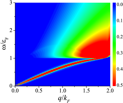
Figure 1: (color online). The contour plot of the dynamic structure factor of a unitary Fermi gas at zero temperature, obtained by using SLDA-RPA. The slope of the low-energy branch is given by the sound speed $c_{s}\simeq 0.354v_{F}$, while the horizontal threshold at $\omega\simeq\varepsilon_{F}$ is equal to the minimum energy $2\Delta$ to break a Cooper-pair. The color bar indicates the value of the dynamic structure factor, which is measured in units of $N/\varepsilon_{F}$ and changes from $0$ (blue) to $0.5$ (red).

In this section, we present the results for the dynamic structure factor of a unitary Fermi gas at zero temperature within SLDA-RPA, and justify our theory at low transferred momentum $q\leq k_{F}$ by comparing the resulting static structure factor Eq. (23) with the latest QMC data Carlson2014 .

Fig. 1 reports a contour plot of $S(\mathbf{q},\omega)$ in the momentum range from $q=0$ to $q=2k_{F}$. Two types of contributions are clearly visible: one is the collective Bogoliubov-Anderson phonon excitations within the energy gap $\omega<E_{g}=2\Delta$ Combescot2006 , which exhibit themselves as a sharp $\delta$-peak in the structure factor spectrum. Right above the energy gap, a much broader distribution emerges, which should be attributed to the fermionic single-particle excitations by breaking Cooper pairs.

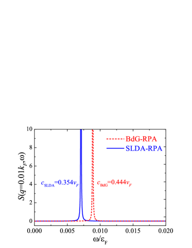
Figure 2: (color online) The phonon peak of the dynamic structure factor of a unitary Fermi gas in the low-$q$ limit. The blue solid line is our SLDA-RPA’s prediction, while the red dashed line is the result from the BdG-RPA theory. Here, to better represent the distribution of a delta function at small $q$, a broadening width $\delta=10^{-4}\varepsilon_{F}$ has been used. The dynamic structure factor is measured in units of $N/\varepsilon_{F}$.

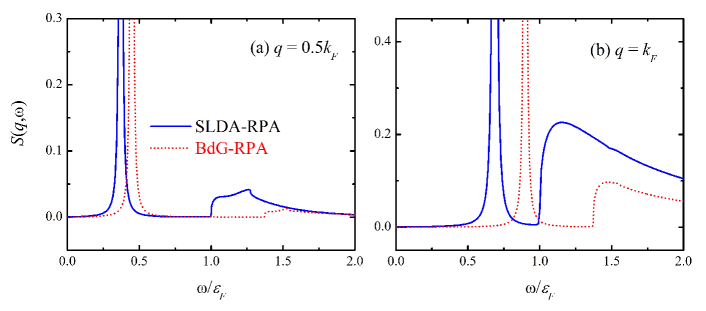
Figure 3: (color online) The dynamic structure factor of a unitary Fermi gas, in units of $N/\varepsilon_{F}$, at $q=0.5k_{F}$ (a) and $q=k_{F}$ (b). The blue solid and red dashed lines show the results of the SLDA-RPA and BdG-RPA theories, respectively. We note that, the scale for the vertical axis in (a) and (b) is different.

A close examination of the phonon excitations is shown in Fig. 2 for a very small transferred momentum $q=0.01k_{F}$. For comparison, we also plot the result of the standard BdG-RPA prediction by a red dashed line. It is anticipated that the dispersion of the phonon excitations should follow $\omega=c_{s}q$, where $c_{s}$ is the sound velocity. By fitting the position of the phonon peak as a function of $q$, we numerically extract a value $c_{s}\simeq 0.354v_{F}$, which coincides, within the accuracy of our numerical calculations, with the value obtained using the macroscopic definition of the sound speed, $c_{s}=\sqrt{(n/m)\partial\mu/\partial n}=\sqrt{\xi_{\mu}/3}v_{F}$. This value is also consistent with the results determined from the experiments and from the ab-initio Monte Carlo calculations. The agreement is not surprising, since the SLDA parameters have been chosen to reproduce the known equation of state and hence the sound speed. It is worth noting that a similar phonon peak is also predicted by the BdG-RPA theory (i.e., using the BdG energy density functional). However, the BdG-RPA theory predicts a sound speed $c_{s}\simeq 0.444v_{F}$, which is about $30\%$ larger than the above mentioned SLDA-RPA result.

At larger transferred momentum, i.e., $q\apprge 0.5k_{F}$, the single-particle excitations start to make a notable contribution to the dynamic structure factor above the threshold $\omega=2\Delta=\varepsilon_{F}$, as shown in Fig. 3. The sharp rise of the single-particle contribution at $\omega=2\Delta$ is unlikely to be destroyed by the possible residue interactions between Cooper pairs and unpaired fermions, which is not accounted for in our theory. Therefore, it could serve as a useful feature to experimentally determine the pairing gap in the two-photon Bragg scattering experiments Vale2016 . We also note that, compared with our SLDA-RPA results, the BdG-RPA theory predicts a much weaker response of the single-particle excitations at a larger threshold. This difference between the SLDA- and BdG-RPA predictions could be easily resolved experimentally.

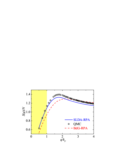
Figure 4: (color online) The static structure factor of a zero-temperature unitary Fermi gas, calculated by the SLDA-RPA theory (blue solid line), in comparison with the QMC result (black circles) Carlson2014 and the BdG-RPA prediction (red dashed line). Our SLDA-RPA theory is expected to be quantitatively reliable at $q\leq k_{F}$, as highlighted by the yellow area.

A test of the accuracy of the theory can be obtained by looking at the static structure factor

$$S(\mathbf{q})=\int d\omega S(\mathbf{q},\omega)$$ (23)

for which for which QMC results are available Carlson2014 ; Combescot2006EPL . The comparison of our SLDA-RPA predictions with the latest diffusion Monte Carlo data Carlson2014 is shown in Fig. 4, together with the predictions of BdG-RPA. The excellent agreement between SLDA-RPA and QMC at $q\leq k_{F}$ is non-trivial and suggests that our theory can be quantitatively reliable at small momentum transfer. Above the Fermi momentum, instead, there are significant deviations. It is worth noticing that the BdG-RPA theory gives results closer to QMC at large momentum transfer, where the physics is dominated by single-particle excitations and where BdG-RPA theory is known to work well Zou2010 .

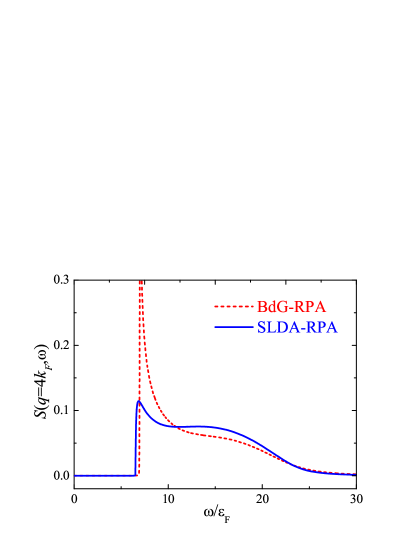
Figure 5: (color) The dynamic structure factor of a zero-temperature unitary Fermi gas (in units of $N/\varepsilon_{F}$) at a large momentum transfer $q=4k_{F}$, calculated by using the SLDA-RPA (blue line) and BdG-RPA theories (red dashed line).

In Fig. 5, we show the dynamic structure factor at the momentum $q=4k_{F}$. At such a large momentum, one can still separately resolve the bosonic Cooper-pair excitations (i.e., a molecular peak structure at $\omega=q^{2}/4m=8\varepsilon_{F}$) and fermionic single-particle excitations (i.e., the broader distribution at $\omega=q^{2}/2m=16\varepsilon_{F}$). Compared with the BdG-RPA result, our SLDA-RPA theory predicts a much smaller molecular peak. This is understandable, since the SLDA theory is effectively a low-energy theory and hence becomes less efficient at $\omega\gg\varepsilon_{F}$. We note that, experimentally, there is a finite energy resolution in the measurement of the dynamic structure factor Zou2010 . The notable difference in the predictions for the molecular peak will be easily smeared out by the finite energy resolution. As a result, the SLDA-RPA approach may predict nearly the same line shape as the BdG-RPA theory. The difference in the line shape is characterized by the relative difference in the static structure factor, which is about $5\%$. In the sense of predicting the experimental line shape for the dynamic structure factor, we may argue that the SLDA-RPA is semi-quantitatively valid at large transferred momentum $q>k_{F}$.

It should also be noted that an independent check of the SLDA-RPA theory is provided by the $f$-sum rule Guo2010

$$\int d\omega\omega S(\mathbf{q},\omega)=\frac{N\mathbf{q}^{2}}{2m},$$ (24)

which should be satisfied. We have numerically checked that our SLDA-RPA calculations obey this sum-rule within $1\%$ relative accuracy.

VI Dynamic structure factor at the BCS-BEC crossover

In this section, we apply the SLDA-RPA theory to determine the dynamic structure factor at the whole BCS-BEC crossover, by using the zero-temperature chemical potential and pairing gap calculated from a Gaussian pair fluctuation theory Hu2006 as the inputs. The energy density functional Eq. (1) - obtained under the scale invariance assumption - is supposed to work well slightly away from the unitary limit.

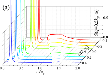
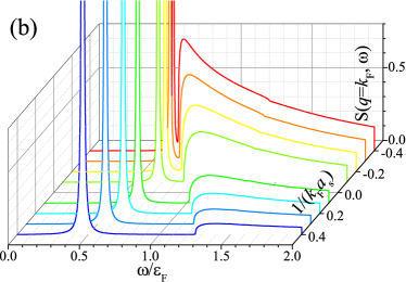
Figure 6: (color online) The dynamic structure factor (in units of $N/\varepsilon_{F}$) at the BCS-BEC crossover and at the tansferred momentum $q=0.5k_{F}$ (a) and $q=k_{F}$ (b).

Fig. 6 reports the dynamic structure factor at the BCS-BEC crossover at two different transferred momenta $q=0.5k_{F}$ (a) and $q=k_{F}$ (b). On the BCS side, the single-particle contributions become significant, as one may anticipate. Furthermore, at $q=k_{F}$ and $1/(k_{F}a)=-0.4$, where the bosonic peak position $\omega_{B}\sim c_{s}q$ is close to the two-particle scattering threshold $2\Delta$, there is a strong overlap between the phonon and single-particle contributions, leading to an interesting peak-dip-bump structure. When the system crosses over to the BEC limit with increasing $1/(k_{F}a)$, the phonon peak moves to the low energy, due to the decreasing sound velocity. The single-particle contributions get suppressed very quickly. In particular, at $q=0.5k_{F}$, the broader single-particle distribution can be barely seen on the BEC side with $1/(k_{F}a)>0$.

Apparently, the experimental determination of the phonon peaks can be ideally used to measure the sound velocity across the BCS-BEC crossover. The measurement of the broader single-particle contributions may also be useful to determine the pairing gap on the BCS side.

VII Conclusions

In summary, we have developed a random phase approximation theory for calculating the dynamic structure factor of a strongly interacting Fermi gas at unitarity and in the BCS-BEC crossover, within the framework of a density functional theory approach Bulgac2007 ; Bulgac2013 . The theory is expected to be quantitatively reliable at low transferred momentum (i.e., $q<k_{F}$) and at low temperature (i.e., $T\ll T_{c}$), where the predicted static structure factor agrees excellently well with the result of the latest ab-initio diffusion quantum Monte Carlo Carlson2014 . Therefore, our theory is useful to understand the dynamic structure factor in the previously un-explored territory of low transferred momentum, as schematically illustrated in Fig. 7 by a red rectangle. A stringent test of the applicability of our theory could be obtained by comparing our predictions with the results of on-going experiments Vale2016 .

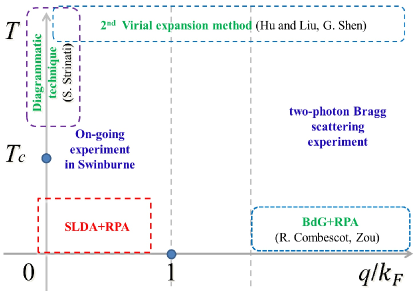
Figure 7: (color online) An illustration of the existing theories of the dynamic structure factor of a strongly interacting Fermi gas, including the virial expansion Hu2010PRA ; Shen2013 , BdG-RPA theory Combescot2006 ; Combescot2006EPL ; Zou2010 and diagrammatic approach Palestini2012 ; He2016 . The applicable parameter space of our SLDA-RPA theory is enclosed by the red dashed line at small transferred momentum $q\leq k_{F}$ and at low temperature $T\ll T_{c}$. The two-photon Bragg scattering experiment has so far been carried out at $q\sim 0.5k_{F}$ Vale2016 and $q\geq 3k_{F}$ Veeravalli2008 ; Lingham2014 . The dashed borders of the domains should not be considered as sharp boundaries, but just as an illustrative guide.

VIII Acknowledgements

We are grateful to Chris Vale, Sandro Stringari, Aurel Bulgac, Michael McNeil Forbes and Lianyi He for fruitful discussions, and Stefano Giorgini and Stefano Gandolfi for sharing their QMC data. PZ is indebted to the BEC Center at Trento for hospitality when this work started. This work was supported by the ARC Discovery Projects: FT130100815 and DP140103231 (HH), DP140100637 , and FT140100003 (XJL). RS acknowledges support from DAE, Government of India. The work is also supported by Provincia Autonoma di Trento (FD). Correspondence should be addressed to PZ at phy.zoupeng@gmail.com.

Appendix A The response function $\chi^{0}$

In this appendix, we discuss how to calculate the response function $\chi^{0}$, by solving the stationary SLDA equation. The existence of four different densities means that there will be 16 correlation functions in $\chi^{0}$:

$$\chi^{0}\equiv\left[\begin{array}[]{cccc}\langle n_{1}n_{1}\rangle_{0}&\langle n_{1}n_{2}\rangle_{0}&\langle n_{1}n_{3}\rangle_{0}&\langle n_{1}n_{4}\rangle_{0}\\ \langle n_{2}n_{1}\rangle_{0}&\langle n_{2}n_{2}\rangle_{0}&\langle n_{2}n_{3}\rangle_{0}&\langle n_{2}n_{4}\rangle_{0}\\ \langle n_{3}n_{1}\rangle_{0}&\langle n_{3}n_{2}\rangle_{0}&\langle n_{3}n_{3}\rangle_{0}&\langle n_{3}n_{4}\rangle_{0}\\ \langle n_{4}n_{1}\rangle_{0}&\langle n_{4}n_{2}\rangle_{0}&\langle n_{4}n_{3}\rangle_{0}&\langle n_{4}n_{4}\rangle_{0}\end{array}\right],$$ (25)

where the abbreviation $\chi_{ij}^{0}=\langle n_{i}n_{j}\rangle_{0}$ is used. The derivation of these matrix elements is cumbersome. We show here, as an example, the derivation of $\chi_{\uparrow\uparrow}^{0}\equiv\chi_{11}^{0}$. According to the Wick theorem, and following the BCS theory, which assume that only propagators - like $\langle\Psi_{\uparrow}^{{\dagger}}\Psi_{\uparrow}\rangle$, $\langle\Psi_{\downarrow}^{{\dagger}}\Psi_{\downarrow}\rangle$, $\langle\Psi_{\downarrow}\Psi_{\uparrow}\rangle$ and $\langle\Psi_{\uparrow}^{{\dagger}}\Psi_{\downarrow}^{{\dagger}}\rangle$ - have a non-zero value, the imaginary-time Green’s function $\chi_{11}^{0}(\textbf{r},\textbf{r}^{\prime},\tau)\equiv-\left\langle T_{\tau}\left[\hat{n}_{1}(\textbf{r},\tau)\hat{n}_{1}(\textbf{r}^{\prime},0)\right]\right\rangle$ can be written as

$$\chi_{11}^{0}=-\left\langle\Psi_{\uparrow}^{\dagger}(\textbf{r},\tau)\Psi_{\uparrow}(\textbf{r}^{\prime},0)\right\rangle\left\langle\Psi_{\uparrow}(\textbf{r},\tau)\Psi_{\uparrow}^{\dagger}(\textbf{r}^{\prime},0)\right\rangle,$$ (26)

where $\tau$ is the imaginary time and we assume $\tau>0$. By using the Bogoliubov transformations

$$\begin{split}\Psi_{\uparrow}&=\sum_{j}\left[u_{j\uparrow}(\textbf{r})c_{j\uparrow}e^{-iE_{j\uparrow}t}+v_{j\downarrow}^{*}(\textbf{r})c_{j\downarrow}^{{\dagger}}e^{iE_{j\downarrow}t}\right],\\ \Psi_{\downarrow}^{{\dagger}}&=\sum_{j}\left[u_{j\downarrow}^{*}(\textbf{r})c_{j\downarrow}^{{\dagger}}e^{iE_{j\downarrow}t}-v_{j\uparrow}(\textbf{r})c_{j\uparrow}e^{-iE_{j\uparrow}t}\right],\end{split}$$ (27)

for the field operators $\Psi_{\sigma}$ and $\Psi_{\sigma}^{{\dagger}}$, one finds

$$\chi_{11}^{0}\left(\textbf{r},\textbf{r}^{\prime},\tau\right)=-\sum_{i,j}u_{i}^{*}(\textbf{r})u_{i}(\textbf{r}^{\prime})u_{j}(\textbf{r})u_{j}^{*}(\textbf{r}^{\prime})f(E_{i})f(-E_{j})e^{(E_{i}-E_{j})\tau}.$$ (28)

Here we use $\langle c_{i}^{\dagger}c_{j}\rangle=f(E_{i})\delta_{ij}$ and $\langle c_{i}c_{j}^{\dagger}\rangle=f(-E_{i})\delta_{ij}$, and $f(x)=1/(e^{x/T}+1)$ is the Fermi distribution function of quasiparticles. The spin index has been removed owing to the existence of a one-to-one correspondence between the solutions of spin-up and spin-down energy levels. By taking the Fourier transformation in the imaginary time, $\chi_{11}^{0}(\textbf{r},\textbf{r}^{\prime},i\nu_{n})=\int_{0}^{\beta}d\tau e^{i\nu_{n}\tau}\chi_{11}^{0}(\textbf{r},\textbf{r}^{\prime},\tau)$, where $\nu_{n}=2n\pi k_{B}T$ is the bosonic Matsubara frequency, one obtains,

$$\chi_{11}^{0}(\textbf{r},\textbf{r}^{\prime},i\nu_{n})=\sum_{i,j}u_{i}^{*}(\textbf{r})u_{i}(\textbf{r}^{\prime})u_{j}(\textbf{r})u_{j}^{*}(\textbf{r}^{\prime})\frac{f(E_{i})-f(E_{j})}{i\nu_{n}+(E_{i}-E_{j})}.$$ (29)

For the homogeneous gas, a set of plane wave functions can be used to expand the eigenfunctions $u_{i}$ in the form $u_{i}(\textbf{r})\rightarrow u_{k}e^{i\textbf{k}\textbf{r}}$. By defining the transferring momentum $\textbf{p}=\textbf{k}^{\prime}-\textbf{k}$ and the relative coordinate $\delta\textbf{r}=\textbf{r}-\textbf{r}^{\prime}$, then

$$\chi_{11}^{0}(\delta\textbf{r},i\nu_{n})=\sum_{\mathbf{k},\mathbf{p}}\left|u_{\mathbf{k}}\right|^{2}\left|u_{\mathbf{k}+\mathbf{p}}\right|^{2}e^{i\textbf{p}\delta\textbf{r}}\frac{f(E_{\mathbf{k}})-f(E_{\mathbf{k}+\mathbf{p}})}{i\nu_{n}+(E_{\mathbf{k}}-E_{\mathbf{k}+\mathbf{p}})}.$$ (30)

By taking the Fourier transformation of the relative coordinate, $\chi_{11}^{0}(q,\omega_{n})=\int d\delta\textbf{r}\chi_{11}^{0}(\delta\textbf{r},i\omega_{n})e^{-i\textbf{q}\delta\textbf{r}}$, we find that,

$$\chi_{11}^{0}(\mathbf{q},i\nu_{n})=\sum_{\mathbf{k}}\left|u_{\mathbf{k}}\right|^{2}\left|u_{\mathbf{k}+\mathbf{p}}\right|^{2}\frac{f(E_{\mathbf{k}})-f(E_{\mathbf{k}+\mathbf{p}})}{i\nu_{n}+(E_{\mathbf{k}}-E_{\mathbf{k}+\mathbf{p}})}.$$ (31)

Using the expressions for $u_{\mathbf{k}}$ and $u_{\mathbf{k}+\mathbf{p}}$, at zero temperature we obtain,

$$\chi_{11}^{0}(\mathbf{q},i\nu_{n})=\sum_{\mathbf{k}}\frac{1}{2}\left(1-\frac{\xi_{\mathbf{k}}\xi_{\mathbf{k}+\mathbf{q}}}{E_{\mathbf{k}}E_{\mathbf{k}+\mathbf{q}}}\right)\frac{E_{\mathbf{k}}+E_{\mathbf{k}+\mathbf{q}}}{\left(i\nu_{n}\right)^{2}-\left(E_{\mathbf{k}}+E_{\mathbf{k}+\mathbf{q}}\right)^{2}}.$$ (32)

Through a similar process, we can derive the other 15 matrix elements of $\chi^{0}$. In fact, after checking their expressions, only six of them are independent. The remaining expressions are simply related to each other by, for example, the replacement $\textbf{k}\rightarrow-\textbf{k}-\textbf{q}$. In the following, we list the other five expressions for $\chi_{12}^{0}$, $\chi_{13}^{0}$, $\chi_{14}^{0}$, $\chi_{34}^{0}$ and $\chi_{43}^{0}$ at zero temperature:

$$\chi_{12}^{0} = \sum_{\mathbf{k}}\frac{1}{2}\frac{\Delta^{2}}{E_{\mathbf{k}}E_{\mathbf{k}+\mathbf{q}}}\frac{E_{\mathbf{k}}+E_{\mathbf{k}+\mathbf{q}}}{(i\nu_{n})^{2}-(E_{\mathbf{k}}+E_{\mathbf{k}+\mathbf{q}})^{2}},$$ (33)

$$\chi_{13}^{0} = \sum_{\mathbf{k}}\frac{\Delta}{4}\left[\frac{\left(\xi_{\mathbf{k}}+\xi_{\mathbf{k}+\mathbf{q}}\right)}{E_{\mathbf{k}}E_{\mathbf{k}+\mathbf{q}}}\frac{E_{\mathbf{k}}+E_{\mathbf{k}+\mathbf{q}}}{(i\nu_{n})^{2}-(E_{\mathbf{k}}+E_{\mathbf{k}+\mathbf{q}})^{2}}-\left(\frac{1}{E_{\mathbf{k}}}+\frac{1}{E_{\mathbf{k}+\mathbf{q}}}\right)\frac{i\nu_{n}}{(i\nu_{n})^{2}-(E_{\mathbf{k}}+E_{\mathbf{k}+\mathbf{q}})^{2}}\right],$$ (34)

$$\chi_{14}^{0} = \sum_{\mathbf{k}}\frac{\Delta}{4}\left[\frac{\left(\xi_{\mathbf{k}}+\xi_{\mathbf{k}+\mathbf{q}}\right)}{E_{\mathbf{k}}E_{\mathbf{k}+\mathbf{q}}}\frac{E_{\mathbf{k}}+E_{\mathbf{k}+\mathbf{q}}}{(i\nu_{n})^{2}-(E_{\mathbf{k}}+E_{\mathbf{k}+\mathbf{q}})^{2}}+\left(\frac{1}{E_{\mathbf{k}}}+\frac{1}{E_{\mathbf{k}+\mathbf{q}}}\right)\frac{i\nu_{n}}{(i\nu_{n})^{2}-(E_{\mathbf{k}}+E_{\mathbf{k}+\mathbf{q}})^{2}}\right],$$ (35)

$$\chi_{34}^{0} = \sum_{\mathbf{k}}\frac{1}{2}\left[\left(1+\frac{\xi_{\mathbf{k}}}{E_{\mathbf{k}}}\frac{\xi_{\mathbf{k}+\mathbf{q}}}{E_{\mathbf{k}+\mathbf{q}}}\right)\frac{E_{\mathbf{k}}+E_{\mathbf{k}+\mathbf{q}}}{(i\nu_{n})^{2}-(E_{\mathbf{k}}+E_{\mathbf{k}+\mathbf{q}})^{2}}+\left(\frac{\xi_{\mathbf{k}}}{E_{\mathbf{k}}}+\frac{\xi_{\mathbf{k}+\mathbf{q}}}{E_{\mathbf{k}+\mathbf{q}}}\right)\frac{i\nu_{n}}{(i\nu_{n})^{2}-(E_{\mathbf{k}}+E_{\mathbf{k}+\mathbf{q}})^{2}}\right],$$ (36)

$$\chi_{43}^{0} = \sum_{\mathbf{k}}\frac{1}{2}\left[\left(1+\frac{\xi_{\mathbf{k}}}{E_{\mathbf{k}}}\frac{\xi_{\mathbf{k}+\mathbf{q}}}{E_{\mathbf{k}+\mathbf{q}}}\right)\frac{E_{\mathbf{k}}+E_{\mathbf{k}+\mathbf{q}}}{(i\nu_{n})^{2}-(E_{\mathbf{k}}+E_{\mathbf{k}+\mathbf{q}})^{2}}-\left(\frac{\xi_{\mathbf{k}}}{E_{\mathbf{k}}}+\frac{\xi_{\mathbf{k}+\mathbf{q}}}{E_{\mathbf{k}+\mathbf{q}}}\right)\frac{i\nu_{n}}{(i\nu_{n})^{2}-(E_{\mathbf{k}}+E_{\mathbf{k}+\mathbf{q}})^{2}}\right].$$ (37)

We note that, $\chi_{34}^{0}$ and $\chi_{43}^{0}$ should be regularized in order to remove the ultraviolet divergence.

References

- (1) I. Bloch, J. Dalibard, and W. Zwerger, Rev. Mod. Phys. 80, 885 (2008).
- (2) A. J. Leggett, Diatomic molecules and Cooper pairs, in Modern Trends in the Theory of Condensed Matter, Lecture Notes in Physics, Vol. 115 (Springer-Verlag, Berlin, 1980).
- (3) S. Giorgini, L. P. Pitaevskii, and S. Stringari, Rev. Mod. Phys. 80, 1215 (2008).
- (4) T.-L. Ho, Phys. Rev. Lett. 92, 090402 (2004).
- (5) H. Hu, P. D. Drummond, and X.-J. Liu, Nature Phys. 3, 469 (2007).
- (6) H. Hu, X.-J. Liu, and P. D. Drummond, New J. Phys. 12, 063038 (2010).
- (7) G. E. Astrakharchik, J. Boronat, J. Casulleras, and S. Giorgini, Phys. Rev. Lett. 93, 200404 (2004).
- (8) A. Bulgac, J. E. Drut, and P. Magierski, Phys. Rev. Lett. 96, 090404 (2006).
- (9) E. Burovski, E. Kozik, N. Prokof’ev, B. Svistunov, and M. Troyer, Phys. Rev. Lett. 101, 090402 (2008).
- (10) J. Carlson and S. Reddy, Phys. Rev. Lett. 95, 060401 (2005).
- (11) J. Carlson and S. Reddy, Phys. Rev. Lett. 100, 150403 (2008).
- (12) J. Carlson, S. Gandolfi, K. E. Schmidt, and S. Zhang, Phys. Rev. A 84, 061602 (2011).
- (13) M. M. Forbes, S. Gandolfi, and A. Gezerlis, Phys. Rev. Lett. 106, 235303 (2011).
- (14) S. Gandolfi, J. Phys.: Conf. Ser. 529, 012011 (2014).
- (15) J. Carlson and S. Gandolfi, Phys. Rev. A 90, 011601(R) (2014).
- (16) Y. Ohashi and A. Griffin, Phys. Rev. Lett. 89, 130402 (2002); Phys. Rev. A 67, 063612 (2003).
- (17) X.-J. Liu and H. Hu, Phys. Rev. A 72, 063613 (2005).
- (18) Q. Chen, J. Stajic, S. Tan, and K. Levin, Phys. Rep. 412, 1 (2005).
- (19) H. Hu, X.-J. Liu, and P. D. Drummond, Europhys. Lett. 74, 574 (2006).
- (20) R. Haussmann, W. Rantner, S. Cerrito, and W. Zwerger, Phys. Rev. A 75, 023610 (2007).
- (21) R. B. Diener, R. Sensarma, and M. Randeria, Phys. Rev. A 77, 023626 (2008).
- (22) B. C. Mulkerin, X.-J. Liu, and H. Hu, Phys. Rev. A 94, 013610 (2016).
- (23) L. Luo, B. Clancy, J. Joseph, J. Kinast, and J. E. Thomas, Phys. Rev. Lett. 98, 080402 (2007).
- (24) S. Nascimbène, N. Navon, K. J. Jiang, F. Chevy, and C. Salomon, Nature (London) 463, 1057 (2010).
- (25) M. Horikoshi, S. Nakajima, M. Ueda, and T. Mukaiyama, Science 327, 442 (2010).
- (26) N. Navon, S. Nascimbène, F. Chevy, and C. Salomon, Science 328, 729 (2010).
- (27) M. J. H. Ku, A. T. Sommer, L.W. Cheuk, and M.W. Zwierlein, Science 335, 563 (2012).
- (28) H. Hu, A. Minguzzi, X.-J. Liu, and M. P. Tosi, Phys. Rev. Lett. 93, 190403 (2004).
- (29) A. Altmeyer, S. Riedl, C. Kohstall, M. J. Wright, R. Geursen, M. Bartenstein, C. Chin, J. Hecker Denschlag, and R. Grimm, Phys. Rev. Lett. 98, 040401 (2007).
- (30) C. H. Schunck, Y. Shin, A. Schirotzek, M. W. Zwierlein, and W. Ketterle, Science 316, 867 (2007).
- (31) A. Schirotzek, Y. Shin, C.H. Schunck, and W. Ketterle, Phys. Rev. Lett. 101, 140403 (2008).
- (32) P. Massignan, G. M. Bruun, and H. T. C. Stoof, Phys. Rev. A 77, 031601(R) (2008).
- (33) Q. J. Chen and K. Levin, Phys. Rev. Lett. 102, 190402 (2009).
- (34) J. P. Gaebler, J. T. Stewart, T. E. Drake, D. S. Jin, A. Perali, P. Pieri, and G. C. Strinati, Nature Phys. 6, 569 (2010).
- (35) H. Hu, X.-J. Liu, P. D. Drummond, and H. Dong, Phys. Rev. Lett. 104, 240407 (2010).
- (36) R. Combescot, M. Y. Kagan, and S. Stringari, Phys. Rev. A 74, 042717 (2006).
- (37) G. Veeravalli, E. Kuhnle, P. Dyke, and C. J. Vale, Phys. Rev. Lett. 101, 250403 (2008).
- (38) For a recent review, see, for example, H. Hu, Front. Phys. 7, 98 (2012).
- (39) M. G. Lingham, K. Fenech, S. Hoinka, and C. J. Vale, Phys. Rev. Lett. 112, 100404 (2014).
- (40) C. J. Vale, Low-lying excitations in a strongly interacting Fermi gas, invited conference presentation at ICAP 2016.
- (41) L. Pitaevskii and S. Stringari, Bose-Einstein Condensation (Oxford University Press, 2003).
- (42) X.-J. Liu, H. Hu, and P. D. Drummond, Phys. Rev. Lett. 102, 160401 (2009).
- (43) X.-J. Liu, Phys. Rep. 524, 37 (2013).
- (44) H. Hu, X.-J. Liu, and P. D. Drummond, Phys. Rev. A 81, 033630 (2010).
- (45) G. Shen, Phys. Rev. A 87, 033612 (2013).
- (46) D. T. Son and E. G. Thompson, Phys. Rev. A 81, 063634 (2010).
- (47) H. Hu and X.-J. Liu, Phys. Rev. A 85, 023612 (2012).
- (48) H. Hu, E. Taylor, X.-J. Liu, S. Stringari, and A. Griffin, New J. Phys. 12, 043040 (2010).
- (49) H. Guo, C.-C. Chien, and K. Levin, Phys. Rev. Lett. 105, 120401 (2010).
- (50) F. Palestini, P. Pieri, and G. C. Strinati Phys. Rev. Lett. 108, 080401 (2012).
- (51) L. He, Ann. Phys. 373, 470 (2016).
- (52) R. Combescot, S. Giorgini, and S. Stringari, Europhys. Lett. 75, 695 (2006).
- (53) P. Zou, E. D. Kuhnle, C. J. Vale, and H. Hu, Phys. Rev. A 82, 061605(R) (2010).
- (54) H. Guo, C.-C. Chien, and Y. He, J. Low Temp. Phys. 172, 5 (2013).
- (55) A. Bulgac, Phys. Rev. C 65, 051305(R) (2002).
- (56) Y. Yu and A. Bulgac, Phys. Rev. Lett. 90, 222501 (2003).
- (57) A. Bulgac, Phys. Rev. A 76, 040502(R) (2007).
- (58) W. Zwerger (ed.), The BCS-BEC Crossover and the Unitary Fermi Gas, Lecture Notes in Physics, Vol. 836 (Springer-Verlag, Berlin, 2012).
- (59) P. Hohenberg and W. Kohn, Phys. Rev. 136, 864 (1964).
- (60) W. Kohn and L.J. Sham, Phys. Rev. 140, 1133 (1965).
- (61) W. Kohn, Rev. Mod. Phys. 71, 1253 (1999).
- (62) A. Bulgac, Y.-L. Luo, P. Magierski, K. J. Roche, and Y. Yu, Science 332, 1288 (2011).
- (63) A. Bulgac, Annu. Rev. of Nucl. Part. Sci. 63, 97 (2013).
- (64) A. Minguzzi, G. Ferrari, and Y. Castin, Eur. Phys. J. D 17, 49 (2001).
- (65) G. M. Bruun and B. R. Mottelson, Phys. Rev. Lett. 87, 270403 (2001).
- (66) X.-J. Liu, H. Hu, A. Minguzzi, and M. P. Tosi, Phys. Rev. A 69, 043605 (2004).
- (67) S. Stringari, Phys. Rev. Lett. 102, 110406 (2009).
- (68) M. M. Forbes and R. Sharma, Phys. Rev. A 90, 043638 (2014).